| Issue |
A&A
Volume 703, November 2025
|
|
|---|---|---|
| Article Number | A37 | |
| Number of page(s) | 14 | |
| Section | Extragalactic astronomy | |
| DOI | https://doi.org/10.1051/0004-6361/202555132 | |
| Published online | 05 November 2025 | |
From simulations to observations: Methodology and data release of mock TNG50 galaxies at 0.3 < z < 0.7 for WEAVE-StePS
1
Dipartimento di Fisica e Astronomia “G. Galilei”, Università di Padova, Vicolo dell’Osservatorio 3, 35122 Padova, Italy
2
Centro de Astrobiología (CAB), CSIC-INTA, Ctra. de Ajalvir km 4, Torrejón de Ardoz, E-28850 Madrid, Spain
3
INAF – Osservatorio Astronomico di Padova, Vicolo dell’Osservatorio 5, 35122 Padova, Italy
4
Instituto de Astronomía y Ciencias Planetarias, Universidad de Atacama, Copiapó, Chile
5
INAF-Osservatorio Astronomico di Brera, Via Brera 28, I-20121 Milano, Italy
6
Università degli Studi di Milano-Bicocca, Piazza della Scienza, I-20125 Milano, Italy
7
Instituto de Astrofísica de Canarias, IAC, Vía Láctea s/n, E-38205 La Laguna, (S.C. Tenerife), Spain
8
Departamento de Astrofísica, Universidad de La Laguna, E-38200 La Laguna, Tenerife, Spain
9
Department of Physics, Oxford University, Keble Road, Oxford OX1 3RH, UK
10
Università di Salerno, Dipartimento di Fisica “E.R. Caianiello”, Via Giovanni Paolo II 132, 84084 Fisciano, (SA), Italy
11
INAF – Osservatorio Astronomico di Capodimonte, Salita Moiariello 16, 80131 Napoli, Italy
12
INFN – Gruppo Collegato di Salerno – Sezione di Napoli, Dipartimento di Fisica “E.R. Caianiello”, Università di Salerno, Via Giovanni Paolo II, 132, 84084 Fisciano, (SA), Italy
13
Departimento de Física de la Tierra y Astrofísica, Fac. CC. Físicas & Instituto de Física de Partículas y del Cosmos, IPARCOS, Universidad Complutense de Madrid, Plaza de las Ciencias 1, E-28040 Madrid, Spain
14
Isaac Newton Group of Telescopes, Apartado 321, 38700 Santa Cruz de la Palma, Tenerife, Spain
15
Dipartimento di Fisica “G. Occhialini”, Università degli Studi di Milano-Bicocca, Piazza della Scienza 3, I-20126 Milano, Italy
16
National Centre for Nuclear Research, ul. Pasteura 7, 02-093 Warsaw, Poland
17
INAF – Osservatorio di Astrofisica e Scienza dello Spazio di Bologna, Via Piero Gobetti 93/3, I-40129 Bologna, Italy
⋆ Corresponding author: This email address is being protected from spambots. You need JavaScript enabled to view it.
Received:
11
April
2025
Accepted:
16
June
2025
Abstract
Context. The new generation of optical spectrographs, including WEAVE, 4MOST, DESI, and WST, offers huge multiplexing capabilities and excellent spectral resolution. This is an unprecedented opportunity to statistically unveil the details of the star formation histories (SFHs) of galaxies. However, these observations are not easily comparable with the predictions of cosmological simulations.
Aims. Our goal is to build a reference framework for comparing spectroscopic observations with cosmological simulations and to test the currently available tools for deriving the stellar population properties of mock galaxies as well as their SFHs. We focus on the observational strategy of the Stellar Population at intermediate redshift Survey (StePS) carried out with the WEAVE instrument.
Methods. We created mock datasets of ∼750 galaxies at redshifts of z = 0.3, 0.5, and 0.7 from the TNG50 cosmological simulation. We performed radiative transfer calculations using SKIRT and analyzed the spectra with the pPXF algorithm, treating them as if they were real observations.
Results. This work presents the methodology used to generate the mock datasets, providing an initial exploration of stellar population properties (i.e. mass-weighted ages and metallicities) and SFHs of a test sample of three galaxies at z = 0.7 and their descendants at z = 0.5 and 0.3. We show that there is very good agreement between mock WEAVE-like spectra compared to the intrinsic values in TNG50 (average difference of 0.2 ± 0.3 Gyr). We also report that an overall agreement is seen when retrieving the SFHs of galaxies, especially if they form the bulk of their stars on short timescales and at early epochs. While we did identify a tendency to overestimate the weight of old stellar populations in galaxies with complex SFHs, we were able to properly recover the timescales on which galaxies build up 90% of their mass, with almost no difference in the measured and intrinsic cumulative SFHs over the last 4 Gyr.
Conclusions. We have released the datasets concurrently with this publication of this paper, which consist of multi-wavelength imaging and spectroscopic data of ∼750 galaxies at redshift z = 0.3, 0.5, and 0.7. This work provides a fundamental bench-test for forthcoming WEAVE observations, providing the community with realistic mock spectra of galaxies that can be used to test currently available tools for deriving first-order stellar populations parameters (i.e. ages and metallicities) as well as more complex diagnostics, such as mass and SFHs.
Key words: galaxies: evolution / galaxies: formation / galaxies: star formation / galaxies: stellar content
© The Authors 2025
 Open Access article, published by EDP Sciences, under the terms of the Creative Commons Attribution License (https://creativecommons.org/licenses/by/4.0), which permits unrestricted use, distribution, and reproduction in any medium, provided the original work is properly cited.
This article is published in open access under the Subscribe to Open model. This email address is being protected from spambots. You need JavaScript enabled to view it. to support open access publication.
1. Introduction
Large extragalactic campaigns, including Sloan Digital Sky Survey (SDSS; York et al. 2000), have enriched our knowledge of the different galaxy populations in the nearby Universe (e.g. Strateva et al. 2001; Kauffmann et al. 2003; Blanton et al. 2003; Baldry et al. 2004; Gallazzi et al. 2005, 2006; Thomas et al. 2010; Goddard et al. 2017). These observations revealed the existence of a bimodality in the properties of local galaxies (i.e. morphology, colour, spectral type, and star formation) with red, quiescent, early-type galaxies shown to be distinct from blue, star-forming, late-type galaxies. For example, galaxies in the blue cloud of the colour-magnitude diagram show a tight correlation between the integrated star formation rate (SFR) and stellar mass, M⋆, along the so-called star formation main sequence (SFMS; e.g. Brinchmann et al. 2004; Daddi et al. 2007; Whitaker et al. 2012; Rinaldi et al. 2025); meanwhile galaxies in the red sequence exhibit no M⋆–SFR correlation. These two populations are separated by transition galaxies, lying in the so-called green valley (Salim et al. 2007). This segregation of galaxies reflects the heterogeneity of physical processes affecting their evolution. Indeed, the comparison of galaxy properties at different redshifts show that they could experience transformations over cosmic time, mostly due to the cessation of star formation activity and rejuvenation events (Lilly et al. 2013; Vulcani et al. 2015; Mancini et al. 2019; Förster Schreiber & Wuyts 2020; Pérez-González et al. 2023; Le Bail et al. 2024; Carnall et al. 2024).
Our ability to reconstruct the star formation histories (SFHs) of galaxies from their stellar populations is key to tracing their individual evolution and constraining their transformation. In this context, a common approach consists of “archaeologically” reconstructing the SFHs of local galaxies and analyzing key features in their spectra and the possible relation with other galaxy properties (e.g. stellar mass, kinematics, star formation activity, and environment). However, despite the large availability of high-resolution spectra of nearby galaxies, it is still extremely difficult to resolve their complex SFHs, due to the degeneracy between age and metallicity and the slow evolution of low-mass stars in evolved stellar populations (mass-weighted ages > 5 Gyr), typical of the majority of massive galaxies (M⋆ > 1010 M⊙; Gallazzi et al. 2005; Serra & Trager 2007).
Star formation histories at early times can be better constrained at intermediate redshifts, when stellar populations were younger and galaxies contained more massive stars. To date, the Large Early Galaxy Astrophysics Census Survey (LEGA-C; van der Wel et al. 2016) is the best campaign suited to trace SFHs in individual galaxies at intermediate redshift (0.6 < z < 1.0), targeting approximately 3000 spectra with median signal-to-noise ratios of S/N ∼ 20 Å−1 (Straatman et al. 2018). This effort will soon be complemented by the Stellar Population at intermediate redshift Survey (StePS; Iovino et al. 2023a), one of the eight surveys that will be carried out with the WHT Enhanced Area Velocity Explorer (WEAVE; Jin et al. 2024), the new wide-field spectroscopic facility for the 4.2-m William Herschel Telescope (WHT) in the Canary Islands. WEAVE-StePS aims to obtain relatively high-resolution (R ∼ 5000) spectra with typical signal-to-noise ratios of S/N ∼ 10 Å−1 for a sample of ∼25 000 galaxies with magnitudes of mi ≤ 20.5 mag, the majority of which lie in the redshift range 0.3 < z < 0.7 (for details, see Iovino et al. 2023a). Thus, the survey will provide reliable measurements of the emission lines and absorption features in the stellar continuum across a broad wavelength coverage 3660 − 9590 Å for a large sample of galaxies in different environments. As an additional effort, high-quality spectra (S/N ∼ 30 Å−1) for more than 3000 galaxies will be observed with the 4-metre Multi-Object Spectrograph Telescope (4MOST) facility mounted on the Visible and Infrared Survey Telescope for Astronomy (VISTA) as part of the 4MOST-StePS campaign (Iovino et al. 2023b).
This work is driven by the need for a better understanding and characterization of complex physical processes involved in galaxy evolution, which are key ingredients of state-of-the-art cosmological simulations. Moreover, properly comparing the properties of observed and simulated galaxies is becoming crucial for both validating the physics implemented in the models and designing the best observational strategies in extragalactic campaigns. In this context, a powerful tool for investigating the synergy between observations and theory is the so-called forward modeling of data (e.g. Snyder et al. 2015; Rodriguez-Gomez et al. 2019; Costantin et al. 2023; Baes et al. 2024; Euclid Collaboration: Abdurro’uf et al. 2025), which consists of generating and analyzing mock datasets from hydrodynamic simulations. In this work, we created mock datasets mimicking WEAVE-StePS observations, but the same strategy could be also used to create mock observations (i.e. accounting for noise and systematics) that mimic any observational setup and provide crucial constraints on the expected performance of any given facility. These datasets are valuable not only for an apple-to-apple comparison between observations and simulations, but also offer the possibility for simulated-based inference of different pathways of galaxy evolution, which are only accessible following galaxies evolution across cosmic time.
In this work, we present the methodology for creating realistic mock observations from the TNG50 simulation tailored for WEAVE-StePS. In particular, we present the mock noiseless datasets and briefly describe how to account for observational conditions typical of WEAVE-StePS, which will be fully characterized in a companion paper. We test currently available tools for deriving the stellar population properties of mock galaxies as well as their SFHs. We compare the measured age and metallicity of nine example galaxies with the intrinsic values derived from TNG50. Moreover, we measure the differences between their central and integrated properties, looking for possible spatial variations.
The paper is organized as follows. In Sect. 2, we describe the main properties of the TNG50 cosmological simulation and the sample selection. In Sect. 3, we describe the methodology to create the mock datasets. In Sect. 4, we present and discuss our results, while in Sect. 5 we summarize the main conclusions of this work. Throughout this study, we assume a Planck Collaboration XIII (2016) cosmology with H0 = 67.74 km s−1 Mpc−1, Ωm = 0.3089, and ΩΛ = 0.6911. We quote magnitudes in the AB system (Oke & Gunn 1983). All errors are reported as the standard deviation, unless stated otherwise.
2. Data and sample
Motivated by the need for a proper comparison between cosmological simulations and upcoming observations with the WEAVE instrument, we built several mock datasets based on the TNG50-1 simulation and tailored for WEAVE-StePS observations of massive galaxies (M⋆ > 1010.2 M⊙) at redshifts of 0.3 < z < 0.7.
TNG50 is a state-of-the-art cosmological magneto-hydrodynamical galaxy formation simulation from the IllustrisTNG project (Weinberger et al. 2017; Pillepich et al. 2018). The simulation follows the evolution of 2 × 21603 total initial resolution elements within a uniform periodic-boundary cube of 51.7 comoving Mpc per side. The spatial scale is set by a gravitational softening of dark matter and stars as 0.575 comoving kpc until z = 1; it is then fixed to its physical value of 288 pc at z = 1, down to z = 0. We refer to Pillepich et al. (2019) and Nelson et al. (2019) for all details about the sub-grid physics implemented in the simulation.
We followed the WEAVE-StePS selection criteria as described in Iovino et al. (2023a) and select TNG50 galaxies in three redshifts snapshots (i.e. z = [0.3, 0.5, 0.7]), having log(M⋆/M⊙) > [10.28, 10.88, 11.23] and being brigher than mi = 20.5 mag. The sample consists of 764 galaxies, of which 562 are at z = 0.3, 155 at z = 0.5, and 47 at z = 0.7. In our sample, we allow for duplicates, meaning the same galaxy could appear in different redshift snapshots. In Table 1, we summarise the distribution of their main physicalproperties.
Physical properties of selected sample of galaxies.
As an example of our data products, we select three main progenitor branches from the TNG50 merger trees, ensuring that galaxies at redshift z = 0.7 occupy different position in the SFR–M⋆ diagram, and follow their evolution across cosmic time. The physical properties (i.e. stellar mass, half-mass radius, and global SFR of the three progenitors and their descendants) are detailed in Table 2.
Physical properties of three examples of galaxies and their descendants.
Figure 1 shows the evolution of SFR and stellar mass of these three galaxies as a function of redshift. We separate galaxies into the star-forming, green-valley, or quiescent categories following the criteria in Croom et al. (2021) and Vaughan et al. (2022). Galaxy ID 172231 is highly star forming at z = 0.7 and it slowly quenches, evolving into ID 218606 at z = 0.5 (star forming) and into ID 251598 at z = 0.3 (green valley). Galaxy ID 222130 (green valley) evolves into ID 234935 at z = 0.5 (green valley) and into ID 277675 at z = 0.3 (star forming). Galaxy ID 212087 (quiescent) slowly rejuvenates, evolving into ID 253460 at z = 0.5 (green valley) and into ID 298351 at z = 0.3 (star forming). These three examples provide excellent test cases accounting for the variety of complex SFH and the many paths of galaxy evolution. For our test sample, it is worth noting that the descendants share the same SFH of their progenitors, since no major events happens in the evolution of the three example galaxies from z = 0.7 to 0.3.
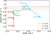 |
Fig. 1. SFR–M⋆ time evolution of the three example galaxies (bigger symbols), from redshift z = 0.7 to 0.3. The galaxy ID follows the nomenclature as in TNG50. Galaxy ID 172231 (blue arrows) slowly quenches (ID 218606) until it reaches the red sequence (ID 251598). Galaxy ID 222130 (green arrows) stays in the green valley (ID 234935) and then moves to the blue cloud sequence (ID 277675). Galaxy ID 212087 (red arrows) slowly rejuvenates (ID 253460) and then moves to the green valley (ID 298351). Dashed lines mark the MS at z = 0.3, 0.5, and 0.7 as defined in Koprowski et al. (2024). |
Figure 2 shows the RGB images of the target galaxies (right panels) and their fibre noiseless spectra (left panels) that we created following the procedure described in Sect. 3. For each set of galaxies, the different rest-frame wavelength covered depends on their redshift. In particular, spectra for galaxies at z = 0.7 reach the bluer part of the spectrum, covering absorption features such as FeII2402, BL2538, FeII2609, and MgII. On the other hand, in galaxies at z = 0.3 we can target the Hα region, which provides the best proxy of star-forming regions. At all redshifts, the Hβ and [OIII]5007 emission lines are available.
It is worth mentioning that in this work we present the main methodology (Sect. 3) and SFH analysis (Sects. 4.1 and 4.2) for three example galaxies at z = 0.7 and their descendants at z = 0.5 and 0.3, discussing their mass-weighted age, metallicity, and formation timescale. While we have chosen to release the full suite of mock spectra with this current paper, our full analysis of the entire sample will be presented in a forthcoming companion paper (Ikhsanova et al., in prep.).
3. Mock datasets
In this section, we describe the strategy we adopted to create mock (realistic) spectra of galaxies, starting with state-of-the-art cosmological simulations. To produce a noiseless mock spectrum, we retrieved the star and gas particles of each selected galaxy in TNG50 and modelled the light distribution of the different stellar populations and star-forming regions, including the effects of dust on radiation. For this task, we employed the SKIRT1 Monte Carlo radiative transfer code (v9.0; Camps & Baes 2020), which was recently used to build mock datasets from different cosmological simulations (Costantin et al. 2023; Barrientos Acevedo et al. 2023; Baes et al. 2024; Nanni et al. 2024).
We followed the strategy described in Costantin et al. (2023), but focusing on a different redshift range. For each galaxy and each snapshot (see Sect. 2), we extracted the corresponding sets of subhalo star particles and gas cells, while the stellar wind particles were ignored. As a note of caution, we needed to adopt several assumptions for the post-processing of the numerical simulations (see e.g. Appendix C). In the following, we follow the standard recipes (i.e. Camps et al. 2016, 2018; Trayford et al. 2017; Rodriguez-Gomez et al. 2019; Kapoor et al. 2021), while using a metallicity-dependent dust-to-metal ratio instead of a constant one (see also Popping et al. 2022).
3.1. Primary source
For the primary source of emission, we assigned to each star particle a spectral energy distribution (SED) that depended on the age and metallicity values extracted from the TNG50 database. To account for the galaxy kinematics, we included the velocity components of each star particle. Each star particle older than 10 Myr was modelled with a simple stellar population (SSP) from the BPASS library (version 2.2.1; Eldridge et al. 2017; Stanway & Eldridge 2018) and a Chabrier (2003) initial mass function (IMF). Each star particle younger than 10 Myr was treated as an unresolved region of the interstellar medium (ISM) and was modelled with an SED from the MAPPINGS III library (Groves et al. 2008), which accounts both for the HII region and for the surrounding photodissociation region.
3.2. Dust modeling
TNG50 does not include the dust physics; hence, we modelled the properties of dust in the ISM using the position, density, and metallicity of the Voronoi gas cells defined through the built-in Voronoi dust grid (Camps et al. 2013). Following Kapoor et al. (2021), the dust component is assumed to be traced by either star-forming (SFR > 0) gas cells or cold gas cells (i.e. with temperature T < 8000 K). The mass of the metals in the ISM is then converted into dust mass with a dust-to-metal ratio using the relation described in Popping & Péroux (2022). To convert TNG50 metallicities to gas-phase metallicities, we assume that oxygen makes up 35% of the metal mass and hydrogen ∼74% of the baryonic mass. The dust mass density of cold and star-forming gas cells is then set to be ρdust = fdustZgasρgas, where Zgas is the metallicity and ρgas is the density of the gas for cold and star-forming gas cells and zero for all the other gas cells.
The dust composition was modeled with the dust mix of Zubko et al. (2004), which includes non-composite silicates, graphite, and neutral and ionized polycyclic aromatic hydrocarbon dust grains. We allowed the dust grains to be stochastically heated and decoupled from local thermal equilibrium, while also including dust self-absorption and re-emission.
3.3. Mock data products
With the recipe described above, we created a set of noiseless mock data products. The spectroscopic mock data set included both fibre spectra centred on the galaxy centre and integral field datacubes encompassing a field of view with diameter equal to one half-mass radius of the dark matter subhalo. In detail, each datacube has a spatial resolution of 0.4 arcsec px−1 and covers the observed spectral range of WEAVE 3660 − 9590 Å with a spectral sampling of 1 Å px−1. Then, each fibre spectrum is extracted from the integral-field datacube by considering only the spaxels within a circular aperture of 1.3 arcsec in diameter, mimicking WEAVE-StePS observations (Iovino et al. 2023a). In Figure 2, we present three showcase galaxies drawn from our sample at z = 0.7 and their descendants at z = 0.5 and 0.3 (nine galaxies in total). These galaxies occupy different places in the SFR–M⋆ diagram (see also Fig. 1 and Sect. 2). We note that we followed the same ID nomenclature as in TNG50, where galaxies can change ID in different snapshots.
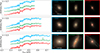 |
Fig. 2. Rest-frame spectra (first column) and RGB images (second to fourth columns) for three example galaxies at redshift z = 0.7 (top row), z = 0.5 (middle row), and z = 0.3 (bottom row), respectively. The first column demonstrates fibre spectra extracted from the central 1.3 arcsec of each galaxy, with arbitrary offset applied in the flux (linear units). In each panel of the first column: green spectra are extracted from galaxy ID 222130, ID 234935, and ID 277675, respectively; blue spectra from galaxy ID 172231, ID 218606, and ID 251598, respectively; red spectra from galaxy ID 212087, ID 253460, and ID 298351, respectively. The fibre size and corresponding physical size are also shown. |
In addition to the spectroscopic dataset, we defined a mock imaging dataset obtained by convolving SKIRT flux densities with the response curve for multiple filters. We created SDSS (ugriz) images with spatial resolution of 0.396 arcsec px−1, ACS/WFC3 (F435W, F606W, F814W, F105W, F125W, and F160W) images with spatial resolution of 0.03 and 0.06 arcsec px−1, and NIRCam (F090W, F115W, F150W, F200W, F277W, F356W, and F444W) images with native spatial resolution of 0.031 and 0.063 arcsec px−1 for the short and long channel, respectively. In Appendix A, we show the imaging dataset for galaxy ID 172231. As an additional product, we built composite RGB images using HST/WFC3 F435W, F606W, and F814W as red, green, and blue layers, respectively. An example of these composite images can be seen in Figure 2. It is worth noting that this work focuses on the analysis of spectroscopic datasets, while the complementary imaging dataset will provide invaluable legacy value to further characterise the properties of these galaxies and their morphological transformation.
3.4. StePS-like data products
Since our goal here is to reproduce realistic mock observations of TNG50 galaxies, we chose to mimic the observational strategy of WEAVE-StePS by perturbing the mock spectra to account for seeing, noise, and spectral resolution effects. Firstly, we convolved each spectral slice of the mock datacube with a Gaussian function of FWHM = 0.69 arcsec, corresponding to the typical seeing for the WHT (Wilson et al. 1999). Then, we extracted a spectrum within a circular aperture centred on the galaxy with a diameter of 1.3 arcsec. Finally, we followed the recipe described in Costantin et al. (2019) and Ditrani et al. (2023), perturbing each fibre spectrum, while accounting for the combined response curve of the WHT and that of the WEAVE spectrograph, the Poisson contribution due to source and sky background, and the readout noise of the WEAVE CCDs. In particular, the sky noise was computed assuming typical conditions of dark nights in La Palma (surface brightness V ∼ 22 mag arcsec−2; Benn & Ellison 1998), while the read-out noise was assumed to be ∼2.5 e− px−1 (Dalton et al. 2016). Since StePS observing strategy consists of short exposures (∼20 min), we neglected the contribution of thermal noise due to dark current (< 0.1 e− h−1). Each noise contribution was added in quadrature to estimate the total noise, which was used as the σ of a Gaussian distribution to perturb each normalized spectrum. While in this work, we focus on mass-weighted ages and metallicities derived from noiseless spectra (Sect. 4.1), in a forthcoming companion paper, we will present the effect of S/N in retrieving the main stellar population properties of the entire sample.
4. Results and discussion
In this section, we describe the methodology we used to create and analyze mock observations of intermediate-redshift galaxies tailored for WEAVE-StePS. Firstly, we quantified possible biases in terms of observing galaxies with limited spatial information, looking at their central and integrated properties. We tested currently available tools for deriving the stellar population properties of mock galaxies and compared the measured age and metallicity of nine example galaxies with the intrinsic values derived from TNG50. Finally, we compared the timescale of star formation from the mix of different stellar populations both in simulations and observations.
4.1. Mass-weighted age and metallicity
We retrieved the mass-weighted age and metallicity of our example galaxies, comparing the observed values with the intrinsic ones obtained from the simulation. Furthermore, we compared how these quantities vary if we analyze the spectrum of the entire galaxy or just the central 1.3 arcsec.
4.1.1. TNG50
We compared the age and metallicity of the entire subhalo in TNG50 with the values obtained for the central aperture. The latter is done by selecting all the star particles within a circular aperture of 1.3 arcsec. We then weighted the age and metallicity distribution of the star particles according to their mass.
In Table 3 (columns 4–5), it can be seen that the average difference in the mass-weighted age between the central region and the entire galaxy is usually small (average of ∼0.4 Gyr), although the core is systematically older than the entire galaxy. This is consistent with the majority of star formation taking place in the disk while the bulge and nuclear region consists of a more mature stellar population, in agreement with an inside-out growth scenario (e.g. Nelson et al. 2021; Costantin et al. 2021, 2022). A similar trend is observed in the metallicity difference (Table 3, columns 8–9), with the central region being systematically more metal-rich than the entire galaxy (average of ∼0.2 dex).
Mass-weighted ages and metallicities of the example galaxies.
It is worth noticing that when using a fixed aperture, at z = 0.7, we are probing larger physical scales (9.56 kpc) compared to z = 0.3 (5.97 kpc). Thus, the contamination from the mixed bulge and disk populations are more significant at the highest redshifts. The average age difference is 0.21 ± 0.12 Gyr at z = 0.7 and 0.61 ± 0.33 Gyr at z = 0.3.
4.1.2. Mock observations
With respect to real galaxies, we analyzed each mock spectrum with the Penalized Pixel-Fitting algorithm (pPXF; Cappellari 2017, 2023) and derived the non-parametric SFH of each galaxy, modelling both the stellar and gas components. We fit the spectra with the BPASS library and Chabrier IMF (Chabrier 2003), consistently with our strategy outlined in Sect. 3.1. The wavelength grid has a resolution of 1 Å over the full range. We consider models with stellar ages from 50 Myr to the age of the Universe at each considered redshift in 24, 23, and 22 bins at z = 0.3, 0.5, and 0.7, respectively and metallicities with the same setup as adopted in Cappellari (2023), in 10 bins with [Z/H] = [−1.3, −1, −0.8, −0.7, −0.5, −0.4, −0.3, 0, 0.2, 0.3] dex. It is worth noticing that the TNG50 star particles may have metallicities above the upper limit of the templates, as already discussed in Sarmiento et al. (2023).
First, we ran pPXF to measure the stellar kinematics (i.e. line-of-sight velocity and velocity dispersion) of each galaxy. Then, we run pPXF again, fixing the kinematics to the values obtained in the first iteration to avoid degeneracies with the stellar population parameters (Sánchez-Blázquez et al. 2011; Martín-Navarro et al. 2024). If the analysis covers noisy spectra, the noise should be scaled according to the residuals of the first fit to achieve a reduced χν2 = 1. This scaling is required to explore various regularized solutions for the best-fitting weight distribution (see Cappellari 2017, 2023, for more details), aimed at identifying the optimal one (i.e. reg ∼ 10 − 750 in this case). To better account for young stellar populations and episodes of intense star formation, we derived weights representing light fractions (e.g. we normalisd the templates to the V-band prior to fitting) and converted them to mass afterwards. We did not apply any additive or multiplicative polynomial.
Following Kacharov et al. (2018), we performed a bootstrap analysis to estimate the uncertainties in the distribution of the mass weights. We sampled each spectrum 100 times using the residuals of the best-fitting regularized solution. Then, each spectrum is fitted with the same setup but without regularisation to avoid self-similarity due to smooth solutions.
Following the procedure described above, we fit both the integrated and StePS-like fibre spectra of each galaxy. From the second pPXF run, we obtain the mean stellar age, metallicity, and SFH of each galaxy (Table 3). The results of the spectral fitting for the three progenitor galaxies (i.e. ID 172231, ID 212087, and ID 222130) are shown in Fig. B.1.
In Figure 3, we compare the two-dimensional distribution of pPXF weights derived for the fibre noiseless spectra in the age-metallicity diagram with the distribution of ages and metallicities derived from the simulation. We find a good agreement in the mass-weighted ages of the example galaxies. For the fibre spectra, the values of age inferred from pPXF agree with the intrinsic ones, with an average difference of 0.2 ± 0.3 Gyr. We find a similar trend for the integrated spectra, with measured ages compatible with intrinsic ones (average difference of 0.6 ± 0.6 Gyr). Regarding metallicities, we find that measured values are systematically lower than the intrinsic ones, with the caveat that we are unable to retrieve metallicities as high as [Z/H] ∼ 0.3 dex. The average difference is 0.3 ± 0.2 dex between the fibre and integrated spectra.
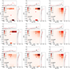 |
Fig. 3. Distribution of the pPXF weights (red colours), indicating the mass fraction of each stellar population of given age and metallicity, derived from fibre noiseless spectra. The mass-weighted age and metallicity measured with pPXF is shown as a red star, while mass-weighted age and metallicity derived from the simulation is marked as a black star. Black lines represent the marginalised distribution of ages and metallicities derived from the simulation, while red curves show those inferred from pPXF. The progenitor galaxies at z = 0.7 are shown in the top row, while their descendants at z = 0.5 and z = 0.3 are shown in the middle and bottom rows, respectively. |
Overall, our analysis suggests that there is a good agreement in the inference of mass-weighted ages, even if we tend to predict lower metallicities for the galaxies. This can also be seen in the marginalised age and metallicity distribution (Fig. 3). In a companion paper, we aim to statistically quantify these specific trends for the selected population described in Sect. 2, also considering the effect of S/N in observations.
4.2. Star formation history
Thanks to TNG50, we have full access to the variety of SFHs and stellar, gas, and dark matter properties of our sample galaxies. In Figure 4 (top row), we can appreciate the complexity of the SFH of the three example galaxies, which are characterised by multiple episodes of intense star formation.
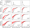 |
Fig. 4. Examples of SFHs (first row) and cumulative SFHs of the target galaxies at redshift z = 0.7 (second row), z = 0.5 (third row), and z = 0.3 (fourth row). The SFHs are derived directly from the cosmological simulation and represent the sum of the SFRs of all progenitors at each snapshot. The cumulative SFHs of each galaxy are retrieved by fitting with pPXF both the StePS-like fibre spectra (red solid line) and integrated noiseless spectra (red dashed line). The shaded red regions indicate the 16th–84th percentile range across 100 bootstrap realisations. For comparison, the cumulative SFHs derived directly from the cosmological simulation are shown both for the entire galaxy (black dashed line) and for the central 1.3 arcsec (black solid line). |
To bridge the gap between theoretical and observational descriptions of the SFH of galaxies, we analyse the noiseless spectra and compare the SFHs of our galaxies retrieved from pPXF with those inferred from the simulation. To visualise the burstiness of the SFH, we computed the sum of the star formation rates (SFRs) of all progenitors at each snapshot, as shown in the first row of Fig. 4. In the second to fourth rows, we describe the SFH as the cumulative mass fraction over cosmic time. From TNG50 (Fig. 4, black lines), we derived the cumulative SFH of each galaxy by integrating across cosmic time the normalized mass-weighted age of each star particle either in the entire galaxy (dashed black line) or in the central 1.3 arcsec (solid black line). For the noiseless mock spectra (Fig. 4, red lines), we marginalised the age weights obtained from pPXF over the metallicity and integrated them across cosmic time. From the recovered cumulative SFHs, we derive t10, t50, and t90 as the time when the galaxy formed 10%, 50%, and 90% of its stellar mass (Table 4).
Timescale of mass assembly of the example galaxies derived from the central 1.3 arcsec.
The three progenitor galaxies (and their descendants) have very different SFHs: galaxy ID 212087 formed its stars over a short period of time (z ∼ 4.5), when the Universe was only 1.3 Gyr old; ID 222130 had one prominent burst at z ∼ 3 (age of the Universe of 2.1 Gyr) and a residual star formation over a few gigayears (Gyr) down to z ∼ 0.3; ID 172231 shows a very bursty evolution with an extended period of intense bursts (SFR > 100 M⊙ yr−1 from z = 2.3 to z = 1.3 (age of the Universe from 2.8 to 4.8 Gyr) and mild residual star formation during a few Gyr until it quenches at z ∼ 0.3.
We find that if the galaxy forms at early cosmic times in a single burst, such as ID 212087, there is almost a perfect agreement between the intrinsic and inferred cumulative SFH (Fig. 4, third column). This suggests that galaxies forming in one single episode have simpler stellar populations (e.g. Pappalardo et al. 2021). In general, if the dominant burst is older than ∼5 Gyr, the inferred stellar populations are massively old (see also Grèbol-Tomàs et al. 2023). The difference between intrinsic and measured cumulative SFH is higher for prolonged and very bursty SFHs (e.g. ID 172231). In all cases, we find that the percentage of mass formed in the first Gyr is greater than 25%, while the intrinsic values could be as low as 2−5%. Despite this systematic trend, which reflects the fact that we are not sensitive to the shape of the SFH, there is better agreement in the timescale when the galaxies formed almost the totality of its stellar mass, especially at the highest redshifts, reflecting the fact that we are very sensitive to the timescale of the main quenching event.
We find that the example galaxies and their descendants have similar t90 at all redshifts (average difference of 0.4 ± 0.6 Gyr). However, galaxies can show different t10 and t50, with inferred values being older than intrinsic ones (average difference of 0.8 ± 0.5 Gyr and 1.2 ± 0.5 Gyr). Again, this reflects the fact that we are overestimating the fraction of mass forming in the first phases of galaxy evolution, especially when they have complex SFHs. This trend is partially mitigated once comparing the assigned values during the radiative transfer modeling to the inferred ones (see Appendix C). Finally, we calculate the symmetric mean absolute percentage error for all galaxies in bins of 1 Gyr (lookback time). We notice that there is an almost perfect agreement between the predicted and measured trends of SFH in a lookback time of 4 Gyr (average values < 5%), except for galaxyID 172231.
5. Summary and conclusions
We used the radiative transfer code SKIRT to create mock spectroscopic and imaging datasets of galaxies from the TNG50 cosmological simulation. This dataset represents the ideal solution for comparing forthcoming WEAVE-like observations with cosmological simulations. We describe the methodology for creating the mock datasets in this work and release them to the public concurrently with this work.
Furthermore, we analyzed three showcase galaxies at z = 0.7 and their descendants at z = 0.5 and 0.3, deriving their mass-weighted age, metallicity, and SFH. We compared the intrinsic stellar population properties to those inferred using pPXF, finding that there is an overall good agreement in retrieving the cumulative SFH of the showcased galaxies. In particular, we are very sensitive to the timescale when galaxies build up the bulk of their stellar mass, with a ≲5% average difference in the cumulative SFH estimations across a lookback time of 4 Gyr (except for galaxy ID 172231). Based on the trend derived from the three example galaxies presented in this work (selected for the diversity of their SFHs), we derived compatible ages but lower metallicities compared to the intrinsic age-metallicity distribution retrieved from TNG50. The analysis of the entire sample of galaxies (to be presented in a companion paper) will allow us to statistically explore all the possible systematics addressed in this work. It is worth stressing that, while our work relies on the sample selection criteria and observational setup of WEAVE-StePS, the noiseless datasets can be used to mimic the observational setup of any facility. Furthermore, the spectroscopic information can be combined with the imaging dataset, adding valuable information about the interplay between the mass build up and the morphological transformation of galaxies as well as reducing the age-metallicity degeneracy that could hamper our understanding of mass build-up in the early stages of galaxy evolution.
In conclusion, these mock observations can be used for quantifying possible biases (and the correcting factors) in deriving the SFHs of galaxies. In addition, they enable proper comparisons of the ages, metallicities, and star formation timescales for observed and simulated galaxies.
Data availability
The mock datasets released are available at: https://doi.org/10.5281/zenodo.15862207
SKIRT documentation: http://www.skirt.ugent.be
Acknowledgments
We would like to thank the anonymous referee for all the comments that improved the content of the manuscript. We thank D. Bettoni for the relevant comments during the internal review of the manuscript. We wish to thank S. Jin for her careful reading of the draft that helped to improve this paper. We would like to thank M. Baes for the valuable discussion about SKIRT modeling. This project has received funding from the European Union’s Horizon 2020 research and innovation programme under the Marie Skłodowska-Curie Grant Agreement No. 101034319 and from the European Union – NextGenerationEU. The project that gave rise to these results received the support of a fellowship from the “la Caixa” Foundation (ID 100010434). The fellowship code is LCF/BQ/PR24/12050015. LC acknowledges support from grants PID2022-139567NB-I00 and PIB2021-127718NB-I00 funded by the Spanish Ministry of Science and Innovation/State Agency of Research MCIN/AEI/10.13039/501100011033 and by “ERDF A way of making Europe”. AFM acknowledges support from RYC2021-031099-I and PID2021-123313NA-I00 of MICIN/AEI/10.13039/501100011033/FEDER, UE, NextGenerationEU/PRT. EMC and AP are supported by the Istituto Nazionale di Astrofisica (INAF) through the grant Progetto di Ricerca di Interesse Nazionale (PRIN) 2022 2022383WFT “SUNRISE” (CUP C53D23000850006) and Padua University with the grants Dotazione Ordinaria Ricerca (DOR) 2021-2023. A.I., F.D., M.L. and S.Z. acknowledge financial support from INAF Mainstream grant 2019 WEAVE StePS 1.05.01.86.16 and INAF Large Grant 2022 WEAVE StePS 1.05.12.01.11. PSB acknowledges support from Grant PID2022-138855NB-C31 funded by MICIU/AEI/10.13039/501100011033 and by ERDF/EU. R.R. acknowledges financial support grants through INAF-WEAVE StePS founds and through PRIN-MIUR 2020SKSTHZ. C.P.H. acknowledges support from ANID through Fondecyt Regular project number 1252233. Funding for the WEAVE facility has been provided by UKRI STFC, the University of Oxford, NOVA, NWO, Instituto de Astrofísica de Canarias (IAC), the Isaac Newton Group partners (STFC, NWO, and Spain, led by the IAC), INAF, CNRS-INSU, the Observatoire de Paris, Région Île-de-France, CONACYT through INAOE, the Ministry of Education, Science and Sports of the Republic of Lithuania, Konkoly Observatory (CSFK), Max-Planck-Institut für Astronomie (MPIA Heidelberg), Lund University, the Leibniz Institute for Astrophysics Potsdam (AIP), the Swedish Research Council, the European Commission, and the University of Pennsylvania. The WEAVE Survey Consortium consists of the ING, its three partners, represented by UKRI STFC, NWO, and the IAC, NOVA, INAF, GEPI, INAOE, Vilnius University, FTMC – Center for Physical Sciences and Technology (Vilnius), and individual WEAVE Participants. Please see the relevant footnotes for the WEAVE website (https://weave-project.atlassian.net/wiki/display/WEAVE) and for the full list of granting agencies and grants supporting WEAVE (https://weave-project.atlassian.net/wiki/display/WEAVE/WEAVE+Acknowledgements).
References
- Baes, M., Gebek, A., Trčka, A., et al. 2024, A&A, 683, A181 [NASA ADS] [CrossRef] [EDP Sciences] [Google Scholar]
- Baldry, I. K., Glazebrook, K., Brinkmann, J., et al. 2004, ApJ, 600, 681 [Google Scholar]
- Barrientos Acevedo, D., van der Wel, A., Baes, M., et al. 2023, MNRAS, 524, 907 [NASA ADS] [CrossRef] [Google Scholar]
- Benn, C. R., & Ellison, S. L. 1998, New Astron. Rev., 42, 503 [Google Scholar]
- Blanton, M. R., Hogg, D. W., Bahcall, N. A., et al. 2003, ApJ, 594, 186 [NASA ADS] [CrossRef] [Google Scholar]
- Brinchmann, J., Charlot, S., White, S. D. M., et al. 2004, MNRAS, 351, 1151 [Google Scholar]
- Camps, P., & Baes, M. 2020, Astron. Comput., 31, 100381 [NASA ADS] [CrossRef] [Google Scholar]
- Camps, P., Baes, M., & Saftly, W. 2013, A&A, 560, A35 [NASA ADS] [CrossRef] [EDP Sciences] [Google Scholar]
- Camps, P., Trayford, J. W., Baes, M., et al. 2016, MNRAS, 462, 1057 [CrossRef] [Google Scholar]
- Camps, P., Trčka, A., Trayford, J., et al. 2018, ApJS, 234, 20 [NASA ADS] [CrossRef] [Google Scholar]
- Cappellari, M. 2017, MNRAS, 466, 798 [Google Scholar]
- Cappellari, M. 2023, MNRAS, 526, 3273 [NASA ADS] [CrossRef] [Google Scholar]
- Carnall, A. C., Cullen, F., McLure, R. J., et al. 2024, MNRAS, 534, 325 [NASA ADS] [CrossRef] [Google Scholar]
- Chabrier, G. 2003, PASP, 115, 763 [Google Scholar]
- Costantin, L., Iovino, A., Zibetti, S., et al. 2019, A&A, 632, A9 [NASA ADS] [CrossRef] [EDP Sciences] [Google Scholar]
- Costantin, L., Pérez-González, P. G., Méndez-Abreu, J., et al. 2021, ApJ, 913, 125 [NASA ADS] [CrossRef] [Google Scholar]
- Costantin, L., Pérez-González, P. G., Méndez-Abreu, J., et al. 2022, ApJ, 929, 121 [NASA ADS] [CrossRef] [Google Scholar]
- Costantin, L., Pérez-González, P. G., Vega-Ferrero, J., et al. 2023, ApJ, 946, 71 [NASA ADS] [CrossRef] [Google Scholar]
- Croom, S. M., Taranu, D. S., van de Sande, J., et al. 2021, MNRAS, 505, 2247 [CrossRef] [Google Scholar]
- Daddi, E., Dickinson, M., Morrison, G., et al. 2007, ApJ, 670, 156 [NASA ADS] [CrossRef] [Google Scholar]
- Dalton, G., Ham, S. J., Trager, S., et al. 2016, SPIE Conf. Ser., 9913, 99132X [Google Scholar]
- Ditrani, F. R., Longhetti, M., La Barbera, F., et al. 2023, A&A, 677, A93 [NASA ADS] [CrossRef] [EDP Sciences] [Google Scholar]
- Eldridge, J. J., Stanway, E. R., Xiao, L., et al. 2017, PASA, 34, e058 [Google Scholar]
- Euclid Collaboration (Abdurro’uf, et al.) 2025, A&A, 702, A72 [Google Scholar]
- Förster Schreiber, N. M., & Wuyts, S. 2020, ARA&A, 58, 661 [Google Scholar]
- Gallazzi, A., Charlot, S., Brinchmann, J., White, S. D. M., & Tremonti, C. A. 2005, MNRAS, 362, 41 [Google Scholar]
- Gallazzi, A., Charlot, S., Brinchmann, J., & White, S. D. M. 2006, MNRAS, 370, 1106 [Google Scholar]
- Goddard, D., Thomas, D., Maraston, C., et al. 2017, MNRAS, 466, 4731 [NASA ADS] [Google Scholar]
- Grèbol-Tomàs, P., Ferré-Mateu, A., & Domínguez-Sánchez, H. 2023, MNRAS, 526, 4024 [CrossRef] [Google Scholar]
- Groves, B., Dopita, M. A., Sutherland, R. S., et al. 2008, ApJS, 176, 438 [NASA ADS] [CrossRef] [Google Scholar]
- Iovino, A., Poggianti, B. M., Mercurio, A., et al. 2023a, A&A, 672, A87 [NASA ADS] [CrossRef] [EDP Sciences] [Google Scholar]
- Iovino, A., Mercurio, A., Gallazzi, A. R., et al. 2023b, The Messenger, 190, 22 [NASA ADS] [Google Scholar]
- Jin, S., Trager, S. C., Dalton, G. B., et al. 2024, MNRAS, 530, 2688 [NASA ADS] [CrossRef] [Google Scholar]
- Kacharov, N., Neumayer, N., Seth, A. C., et al. 2018, MNRAS, 480, 1973 [Google Scholar]
- Kapoor, A. U., Camps, P., Baes, M., et al. 2021, MNRAS, 506, 5703 [NASA ADS] [CrossRef] [Google Scholar]
- Kauffmann, G., Heckman, T. M., White, S. D. M., et al. 2003, MNRAS, 341, 33 [Google Scholar]
- Koprowski, M. P., Wijesekera, J. V., Dunlop, J. S., et al. 2024, A&A, 691, A164 [NASA ADS] [CrossRef] [EDP Sciences] [Google Scholar]
- Le Bail, A., Daddi, E., Elbaz, D., et al. 2024, A&A, 688, A53 [NASA ADS] [CrossRef] [EDP Sciences] [Google Scholar]
- Lilly, S. J., Carollo, C. M., Pipino, A., Renzini, A., & Peng, Y. 2013, ApJ, 772, 119 [NASA ADS] [CrossRef] [Google Scholar]
- Mancini, C., Daddi, E., Juneau, S., et al. 2019, MNRAS, 489, 1265 [Google Scholar]
- Martín-Navarro, I., de Lorenzo-Cáceres, A., Gadotti, D. A., et al. 2024, A&A, 684, A110 [NASA ADS] [CrossRef] [EDP Sciences] [Google Scholar]
- Nanni, L., Neumann, J., Thomas, D., et al. 2024, MNRAS, 527, 6419 [Google Scholar]
- Nelson, D., Pillepich, A., Springel, V., et al. 2019, MNRAS, 490, 3234 [Google Scholar]
- Nelson, E. J., Tacchella, S., Diemer, B., et al. 2021, MNRAS, 508, 219 [NASA ADS] [CrossRef] [Google Scholar]
- Oke, J. B., & Gunn, J. E. 1983, ApJ, 266, 713 [NASA ADS] [CrossRef] [Google Scholar]
- Pappalardo, C., Cardoso, L. S. M., Michel Gomes, J., et al. 2021, A&A, 651, A99 [NASA ADS] [CrossRef] [EDP Sciences] [Google Scholar]
- Pérez-González, P. G., Barro, G., Annunziatella, M., et al. 2023, ApJ, 946, L16 [CrossRef] [Google Scholar]
- Pillepich, A., Springel, V., Nelson, D., et al. 2018, MNRAS, 473, 4077 [Google Scholar]
- Pillepich, A., Nelson, D., Springel, V., et al. 2019, MNRAS, 490, 3196 [Google Scholar]
- Planck Collaboration XIII. 2016, A&A, 594, A13 [NASA ADS] [CrossRef] [EDP Sciences] [Google Scholar]
- Popping, G., & Péroux, C. 2022, MNRAS, 513, 1531 [CrossRef] [Google Scholar]
- Popping, G., Pillepich, A., Calistro Rivera, G., et al. 2022, MNRAS, 510, 3321 [CrossRef] [Google Scholar]
- Rinaldi, P., Navarro-Carrera, R., Caputi, K. I., et al. 2025, ApJ, 981, 161 [Google Scholar]
- Rodriguez-Gomez, V., Snyder, G. F., Lotz, J. M., et al. 2019, MNRAS, 483, 4140 [NASA ADS] [CrossRef] [Google Scholar]
- Salim, S., Rich, R. M., Charlot, S., et al. 2007, ApJS, 173, 267 [NASA ADS] [CrossRef] [Google Scholar]
- Sánchez-Blázquez, P., Ocvirk, P., Gibson, B. K., Pérez, I., & Peletier, R. F. 2011, MNRAS, 415, 709 [Google Scholar]
- Sarmiento, R., Huertas-Company, M., Knapen, J. H., et al. 2023, A&A, 673, A23 [NASA ADS] [CrossRef] [EDP Sciences] [Google Scholar]
- Serra, P., & Trager, S. C. 2007, MNRAS, 374, 769 [Google Scholar]
- Snyder, G. F., Torrey, P., Lotz, J. M., et al. 2015, MNRAS, 454, 1886 [NASA ADS] [CrossRef] [Google Scholar]
- Stanway, E. R., & Eldridge, J. J. 2018, MNRAS, 479, 75 [NASA ADS] [CrossRef] [Google Scholar]
- Straatman, C. M. S., van der Wel, A., Bezanson, R., et al. 2018, ApJS, 239, 27 [NASA ADS] [CrossRef] [Google Scholar]
- Strateva, I., Ivezić, Ž., Knapp, G. R., et al. 2001, AJ, 122, 1861 [CrossRef] [Google Scholar]
- Thomas, D., Maraston, C., Schawinski, K., Sarzi, M., & Silk, J. 2010, MNRAS, 404, 1775 [NASA ADS] [Google Scholar]
- Trayford, J. W., Camps, P., Theuns, T., et al. 2017, MNRAS, 470, 771 [NASA ADS] [CrossRef] [Google Scholar]
- van der Wel, A., Noeske, K., Bezanson, R., et al. 2016, ApJS, 223, 29 [Google Scholar]
- Vaughan, S. P., Barone, T. M., Croom, S. M., et al. 2022, MNRAS, 516, 2971 [CrossRef] [Google Scholar]
- Vulcani, B., Poggianti, B. M., Fritz, J., et al. 2015, ApJ, 798, 52 [Google Scholar]
- Weinberger, R., Springel, V., Hernquist, L., et al. 2017, MNRAS, 465, 3291 [Google Scholar]
- Whitaker, K. E., van Dokkum, P. G., Brammer, G., & Franx, M. 2012, ApJ, 754, L29 [Google Scholar]
- Wilson, R. W., O’Mahony, N., Packham, C., & Azzaro, M. 1999, MNRAS, 309, 379 [Google Scholar]
- York, D. G., Adelman, J., Anderson, J. E., et al. 2000, AJ, 120, 1579 [Google Scholar]
- Zubko, V., Dwek, E., & Arendt, R. G. 2004, ApJS, 152, 211 [NASA ADS] [CrossRef] [Google Scholar]
Appendix A: Example of mock imaging dataset
As a complementary dataset to the spectroscopic one, for each galaxy we create 18 mock images covering the optical to NIR regime with different spatial resolutions, as detailed in Sect. 3.3. In Fig. A.1, we present an example of the multi-wavelength imaging dataset for galaxy ID 172231.
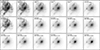 |
Fig. A.1. Example of the multi-wavelength imaging datasets for galaxy ID 172231. |
Appendix B: Example of full-spectral fitting
In Fig. B.1, we report an example of the spectral fitting results performed with pPXF for the three progenitor galaxies at z = 0.7.
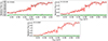 |
Fig. B.1. Example of full spectral fitting performed with pPXF for three galaxies at redshift z = 0.7. The rest-frame noiseless spectra (black solid lines) are plotted with the best-fitting model (orange lines). Each emission line is modelled with one kinematic component. The best-fitting stellar spectrum alone and the gas emissions alone are shown with red and magenta solid lines, respectively. The residuals (green diamonds; arbitrarily offset) are calculated by subtracting the model from the observed spectrum. |
Appendix C: Possible systematics in the radiative transfer modeling
In this appendix, we address the main systematic introduced in the radiative transfer modeling, which has to be kept in mind for a proper comparison between observations and simulations.
In Sect. 3.1, we model each star particle older than 10 Myr with a SSP from the BPASS library. However, once assigning the correspondent SSP within SKIRT, we are limited by the BPASS metallicity grid, which, in particular, does not reproduce the highest metallicities in TNG50. Furthermore, we analyzed the noiseless spectra considering models with stellar ages > 50 Myr using the same procedure as in Cappellari (2023). We tested whether this last choice would not affect our results by repeating the analysis including stellar ages down to 1 Myr and found no systematics in the retrieved stellar population properties.
In Figs. C.1 and C.2, we show the same analysis described in Sects. 4.1.2 and 4.2 but considering also the assigned values together with the intrinsic ones. In this case, the comparison between the assigned values and those retrieved with pPXF show a slightly better agreement in the mass-weighted ages, with an average difference of 0.1 ± 0.3 Gyr. Overall, the assigned SFHs are only slightly closer to the inferred ones, highlighting that part of the systematics are not due to the radiative transfer calculations, especially in the last ∼4 Gyr of galaxy evolution (see also Table C.2).
Mass-weighted ages and metallicities of the central part of the example galaxies extended with assigned values.
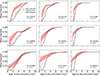 |
Fig. C.2. Same as Fig. 4, but gray solid lines representing assigned values in radiative transfer modeling (i.e. SKIRT) for the fibre spectra. |
Same as Table 4 but extended with assigned values.
All Tables
Timescale of mass assembly of the example galaxies derived from the central 1.3 arcsec.
Mass-weighted ages and metallicities of the central part of the example galaxies extended with assigned values.
All Figures
|
Fig. 1. SFR–M⋆ time evolution of the three example galaxies (bigger symbols), from redshift z = 0.7 to 0.3. The galaxy ID follows the nomenclature as in TNG50. Galaxy ID 172231 (blue arrows) slowly quenches (ID 218606) until it reaches the red sequence (ID 251598). Galaxy ID 222130 (green arrows) stays in the green valley (ID 234935) and then moves to the blue cloud sequence (ID 277675). Galaxy ID 212087 (red arrows) slowly rejuvenates (ID 253460) and then moves to the green valley (ID 298351). Dashed lines mark the MS at z = 0.3, 0.5, and 0.7 as defined in Koprowski et al. (2024). |
| In the text | |
|
Fig. 2. Rest-frame spectra (first column) and RGB images (second to fourth columns) for three example galaxies at redshift z = 0.7 (top row), z = 0.5 (middle row), and z = 0.3 (bottom row), respectively. The first column demonstrates fibre spectra extracted from the central 1.3 arcsec of each galaxy, with arbitrary offset applied in the flux (linear units). In each panel of the first column: green spectra are extracted from galaxy ID 222130, ID 234935, and ID 277675, respectively; blue spectra from galaxy ID 172231, ID 218606, and ID 251598, respectively; red spectra from galaxy ID 212087, ID 253460, and ID 298351, respectively. The fibre size and corresponding physical size are also shown. |
| In the text | |
|
Fig. 3. Distribution of the pPXF weights (red colours), indicating the mass fraction of each stellar population of given age and metallicity, derived from fibre noiseless spectra. The mass-weighted age and metallicity measured with pPXF is shown as a red star, while mass-weighted age and metallicity derived from the simulation is marked as a black star. Black lines represent the marginalised distribution of ages and metallicities derived from the simulation, while red curves show those inferred from pPXF. The progenitor galaxies at z = 0.7 are shown in the top row, while their descendants at z = 0.5 and z = 0.3 are shown in the middle and bottom rows, respectively. |
| In the text | |
|
Fig. 4. Examples of SFHs (first row) and cumulative SFHs of the target galaxies at redshift z = 0.7 (second row), z = 0.5 (third row), and z = 0.3 (fourth row). The SFHs are derived directly from the cosmological simulation and represent the sum of the SFRs of all progenitors at each snapshot. The cumulative SFHs of each galaxy are retrieved by fitting with pPXF both the StePS-like fibre spectra (red solid line) and integrated noiseless spectra (red dashed line). The shaded red regions indicate the 16th–84th percentile range across 100 bootstrap realisations. For comparison, the cumulative SFHs derived directly from the cosmological simulation are shown both for the entire galaxy (black dashed line) and for the central 1.3 arcsec (black solid line). |
| In the text | |
|
Fig. A.1. Example of the multi-wavelength imaging datasets for galaxy ID 172231. |
| In the text | |
|
Fig. B.1. Example of full spectral fitting performed with pPXF for three galaxies at redshift z = 0.7. The rest-frame noiseless spectra (black solid lines) are plotted with the best-fitting model (orange lines). Each emission line is modelled with one kinematic component. The best-fitting stellar spectrum alone and the gas emissions alone are shown with red and magenta solid lines, respectively. The residuals (green diamonds; arbitrarily offset) are calculated by subtracting the model from the observed spectrum. |
| In the text | |
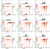 |
Fig. C.1. Same as Fig. 3, but gray stars representing assigned values in SKIRT. |
| In the text | |
|
Fig. C.2. Same as Fig. 4, but gray solid lines representing assigned values in radiative transfer modeling (i.e. SKIRT) for the fibre spectra. |
| In the text | |
Current usage metrics show cumulative count of Article Views (full-text article views including HTML views, PDF and ePub downloads, according to the available data) and Abstracts Views on Vision4Press platform.
Data correspond to usage on the plateform after 2015. The current usage metrics is available 48-96 hours after online publication and is updated daily on week days.
Initial download of the metrics may take a while.