| Issue |
A&A
Volume 703, November 2025
|
|
|---|---|---|
| Article Number | A112 | |
| Number of page(s) | 16 | |
| Section | Cosmology (including clusters of galaxies) | |
| DOI | https://doi.org/10.1051/0004-6361/202555180 | |
| Published online | 13 November 2025 | |
DARKSKIES: A suite of super-sampled zoom-in simulations of galaxy clusters with self-interacting dark matter
1
Laboratoire d’Astrophysique, EPFL, Observatoire de Sauverny, 1290 Versoix, Switzerland
2
Lorentz Institute for Theoretical Physics, Leiden University, PO Box 9506 NL-2300 RA, Leiden, The Netherlands
3
Leiden Observatory, Leiden University, PO Box 9513 NL-2300 RA, Leiden, The Netherlands
4
Institute for Computational Science, University of Zurich, Winterthurerstrasse 190, 8057 Zurich, Switzerland
⋆ Corresponding author: This email address is being protected from spambots. You need JavaScript enabled to view it.
Received:
16
April
2025
Accepted:
28
August
2025
Abstract
We present the ‘DARKSKIES’ suite of one hundred, zoom-in hydrodynamic simulations of massive (M200 > 5 × 10¹⁴ M⊙) galaxy clusters with self-interacting dark matter (SIDM). We super-sampled the simulations such that mDM/mgas ∼ 0.1, enabling us to simulate a dark matter particle mass of m = 0.68 × 10⁸ M⊙ an order of magnitude faster, whilst exploring SIDM in the core of clusters at extremely high resolution. We calibrated the baryonic feedback to produce observationally consistent and realistic galaxy clusters across all simulations and simulated five models of velocity-independent SIDM targeting the expected sensitivity of future telescopes - σDM/m = 0.,0.01, 0.05, 0.1, 0.2 cm2/g. We find that the density profiles exhibit the characteristic core even in the smallest of cross-sections, with cores developing only at late times (z < 0.5). We investigated the dynamics of the brightest cluster galaxy (BCG) inside the dark matter halo and find that in SIDM cosmologies there exists a so-called wobbling not observed in collisionless dark matter. We find that this wobble is driven by mass accreting onto a cored density profile with the signal peaking at z = 0.25 and dropping thereafter. This finding is further supported by the existence of an anti-correlation between the offset between the BCG and the dark matter halo and its relative velocity in SIDM only, a hallmark of harmonic oscillation.
Key words: galaxies: clusters: general / dark matter
© The Authors 2025
 Open Access article, published by EDP Sciences, under the terms of the Creative Commons Attribution License (https://creativecommons.org/licenses/by/4.0), which permits unrestricted use, distribution, and reproduction in any medium, provided the original work is properly cited.
This article is published in open access under the Subscribe to Open model. This email address is being protected from spambots. You need JavaScript enabled to view it. to support open access publication.
1. Introduction
Evidence for a dark, gravitating mass that dominates the matter component of our Universe has been accumulating for almost a century (Zwicky 1933; Rubin et al. 1980; Clowe et al. 2006; Planck Collaboration VI 2020). Despite its abundance in our Universe, no detection has yet been confirmed, with the simplest model – that of a cold and collisionless massive particle that interacts only via gravity – still consistent with observations (hereafter referred to as ‘CDM’, Abbott et al. 2018; Hildebrandt et al. 2017).
In a bid to test theories of dark matter, computational models containing many billion point particles were built, making it possible to see whether changes in the standard dark matter paradigm could lead to plausible Universes. For example, early n-body simulations of pure gravity showed that dark matter must be non-relativistic, with so-called ‘hot dark matter’ being quickly ruled out (Davis et al. 1985, 1981) as it produced too few structures. In fact, the cold and collisionless dark matter model has been incredibly successful at predicting the large-scale distribution of observed galaxies (Springel et al. 2006; Angulo & Hahn 2022).
As observations improved, so did our ability to simulate smaller scales, pushing n-body simulations to reproduce the inner properties of galaxies and galaxy clusters. As a result, discrepancies in the cold and collisionless dark matter model began to appear. For example, dark matter-only simulations predicted the existence of many small structures in the halo of galaxies, coined the ‘missing-satellite’ problem (Kauffmann et al. 1993; Klypin et al. 1999; Moore et al. 1999). Moreover, it appeared that dwarf galaxies harboured flat density profiles in the central parts of the halo, whereas simulations of dark matter predicted cuspy, dense central regions known as the ’core-cusp’ problem (Dubinski & Carlberg 1991; Mateo 1998; de Blok 2010). These problems were quickly followed by other discrepancies between observations and simulations, including the ‘too-big-to-fail’ problem (Boylan-Kolchin et al. 2011). For a long time, these were used as a way to motivate extensions to the CDM paradigm. For example, self-interactions on the dark sector can lead to a dampening of the central region and the production of a dark matter core (Peter et al. 2013). However, it was clear that more sophisticated simulations that included star formation, cooling, and other ‘baryonic processes’1 were required. Including these additional gas physics made it possible to reconcile many of the observed tensions (e.g. Brooks et al. 2013; Pontzen & Governato 2014).
The accuracy of simulations to model the intricate processes of galaxy formation has now advanced to the point where we can simulate large-scale boxes of the Universe and produce realistic objects over many orders of magnitude (Nelson et al. 2018; Schaye et al. 2023; Dolag 2015). These massive simulations are able to simulate a host of different physics, including active galactic nuclei (AGN), neutrinos, and magnetic fields, leading to accurate predictions of observables such as the stellar luminosity function and the gas mass fractions in groups and clusters.
Despite the progress in large-scale simulations, two ‘small-scale problems’ arguably persist. The first is the diversity of rotation curves in galaxies. Current models struggle to predict the variance in the observed rotation curves of galaxies (Oman et al. 2015). The second is the apparent presence of overly concentrated halos - manifested as an anti-correlation between the central dark matter density of dwarf galaxies and their peri-centre distance (Kaplinghat et al. 2019; Despali et al. 2025a), although it has been argued that this anti-correlation is not as strong as previously claimed (Cardona-Barrero et al. 2023). Solutions to these discrepancies could possibly lie in the observations or in the simulated model of CDM and baryons. However, it is possible to relax the assumption that dark matter is collisionless and introduce self-interacting dark matter (SIDM) as a potential solution (Kamada et al. 2017; Nadler et al. 2023). Although a low cross-section (∼10 cm2/g) cannot alter dwarf galaxies in an observable fashion (Harvey et al. 2018), invoking a large self-interaction in the dark sector increases the speed at which the dark matter halo is tidally stripped. This can lead to a process called ‘gravo-thermal collapse’ (Balberg et al. 2002; Koda & Shapiro 2011; Palubski et al. 2024). In this situation, the cooling of the core caused by self-interactions can move energy out of the central region, drawing in more particles and leading to further interactions and cooling. This results in a runaway effect, whereby an overly dense region develops, greater than that found in CDM. Thus, SIDM can produce both cores and cusps. However, some models suggest that even with gravo-thermal collapse, SIDM is unable to recover the observed over-concentrated halos (Li et al. 2025).
Gravo-thermal collapse requires a relatively high cross-section in dwarf galaxies (at the scale of σDM/m ∼ 100 cm2/g), whereas observations of galaxy clusters have already ruled out this possibility with limits of σDM/m < 0.5 cm2/g (Markevitch et al. 2004; Randall et al. 2008; Harvey et al. 2015; Sagunski et al. 2021). Therefore, in order to reconcile these two limits, dark matter must be velocity dependent, such that particles moving in clusters of galaxies (with masses greater than M/M⊙ > 1014) have small cross-sections, and particles in dwarf galaxies (M/M⊙ < 1011) have large cross-sections.
Despite the tentative detections of SIDM in dwarf galaxies, both the limited number of objects and the number of simulations to interpret the data remain the largest obstacles to progress. Galaxy clusters, on the other hand, are numerous and benefit from their ‘gravitational lensing effect’. The mass of a galaxy cluster heavily deforms the space-time around it, distorting the observed images of distant galaxies into correlated arc-like structures (see e.g. Bartelmann & Schneider 2001, for a review). In rare cases, clusters can lead to multiple images of the same galaxy, known as strong gravitational lensing. Both weak and strong gravitational lensing probe the structure of all mass along the line-of-sight, with no assumption of its dynamical state.
Gravitational lensing has been the root of a host of constraints on self-interaction; for example, the first robust constraints2 were from weak gravitational lensing of the bullet cluster (Clowe et al. 2006). Following this, studies of merging clusters (e.g. Merten et al. 2011; Bradač et al. 2008; Williams & Saha 2011; Harvey et al. 2015) with the tightest constraints from Sagunski et al. (2021), who used a sample of clusters and groups to constrain it to σDM/m < 0.35 cm2/g did so without simulations of SIDM. There have been some observations of potential signals of SIDM in clusters with measurements of the offset between dark matter and baryons in relaxed galaxy clusters – an unambiguous signal of dark matter self-interactions where offsets cannot exist in CDM (Schaller et al. 2015a). Harvey et al. (2017) used ten strong lensing galaxy clusters to measure a wobbling amplitude of  kpc. Similarly, both Harvey et al. (2017) and Roche et al. (2024) found that offsets in clusters between the dark matter halo and brightest cluster galaxy (BCG) are consistent with the softening length of the simulation. Indeed, Harvey et al. (2017) attempted to model and de-convolve the impact of softening in order to achieve sub-smoothing length precision. Ultimately, they found that the offsets observed in Harvey et al. (2017) were consistent with zero. However, de-convolving resulted in uncertain predictions and hence, without high-resolution SIDM simulations, it would be impossible to place constraints. This is particularly important as the number of observed clusters will soon rise dramatically with the first observations of the Euclid satellite.
Numerical simulations of SIDM have played a key role in advancing this area of research. Thought to be ruled out by measurements of halo sphericity (Miralda-Escudé 2002), the first large-scale (L > 100 Mpc/h) cosmological simulations of SIDM found that cross-sections of σCM/m ∼ 1 cm2/g were consistent with data (Peter et al. 2013; Rocha et al. 2013). Following this, numerical studies exploring the observable manifestations of SIDM were exclusively dark matter only (DMO) (e.g. Buckley et al. 2014). However, these were limited by their exclusion of baryonic physics, which has a dramatic impact on the core of galaxies and clusters of galaxies. This was changed by the first large-scale, cosmological simulations of SIDM with full baryonic feedback (Robertson et al. 2019). Based on the BAHAMAS simulations (McCarthy et al. 2017, 2018), BAHAMAS-SIDM simulations were a suite of cosmological simulations based on the EAGLE model (Schaye et al. 2015) of star formation, cooling, and AGN feedback (which itself was based on the overwhelmingly large simulations (OWLs) simulation (Schaye et al. 2010). These were calibrated to reproduce the correct gas fraction in groups of galaxies and consisted of a 400 Mpc/h box, with dark matter mass of mDM = 3.85 × 10⁹ M⊙ and an initial gas mass of mgas = 7.66 × 10⁸ M⊙ and a WMAP9 (Bennett et al. 2013) cosmology. These were run with an adapted Gadget-3 smooth particle hydro-dynamics (SPH) solver (Springel 2005) and a gas smoothing length of ϵ = 5.7 kpc. At this scale, they were able to resolve the interactions of dark matter down to the σDM/m = 0.1 cm2/g. However, even at these scales the imprint of the softening could be observed on the characteristic scale at which it interacted. More recent work ran zoom-in cluster simulations with SIDM. For example, the DIANOGO simulations looked at six high-resolution zoom-in simulations (Ragagnin et al. 2024), in which two different models of SIDM were tested: rare (with high momentum exchanged) and frequent (but low momentum exchange) dark matter self-interactions. Simulations of lower mass halos have also been comprehensively explored. For example, the AIDA simulations were extremely high-resolution cosmological boxes of five different dark matter models including warm dark matter and SIDM (Despali et al. 2025b). Leveraging the Illustris-TNG galaxy formation model, AIDA-TNG looks at how dark matter affects the build-up of intermediate mass halos (Despali et al. 2025b). In a similar fashion, the Concerto suite of SIDM simulations aimed at tracing the evolution of SIDM in zoom-in simulations in intermediate mass halos (Nadler et al. 2025) at extremely high resolution (mDM = (103 − 105) M⊙). Finally, SIDM simulations at very small scales have been extensively explored as the dark matter-dominated dwarf galaxies present an exciting environment. The first simulations of SIDM in dwarf galaxies were run by Robles et al. (2017) and Harvey et al. (2018). Following this, further tests with velocity-dependent cross-sections looked at gravo-thermal collapse on the dwarf galaxy scale (Correa et al. 2022).
We build on this body of work and present the first suite of high-resolution dark matter zoom-in simulations of massive galaxy clusters with a super-sampled distribution of dark matter, with a full prescription of independently calibrated baryonic feedback. These simulations are part of the ‘DARKSKIES’ project aimed at constraining the self-interaction cross-section of dark matter to within σDM/m < 0.1 cm2/g. In Section 2 we present the underlying framework and model of our simulations, including how we generated the initial conditions, calibrated the meta-parameters that govern the hydro-dynamics, and selected the models of SIDM to simulate. In Section 3 we present the results of the simulations, and lastly in Section 4 we present our conclusions. Unless otherwise stated, all error bars show the 1σ (68%) confidence limit in a value, and we also assume a Planck cosmology throughout (Planck Collaboration VI 2020).
2. Method
Zoom-in simulations whereby the mass resolution of the system in a particular region is enhanced is an efficient way to simulate individual objects of interest, at high-resolution without wasting computational time on the large-scale surrounding environment. In this section we outline the methodology used to generate the initial conditions and then carry out the simulations. Specific details of the simulations follow. As an overview, we carried out the following procedure:
-
We ran an initial 400 h−1 Mpc large-scale DMO cosmological box from which to select the clusters to re-simulate.
-
We selected 30 galaxy clusters ranging in mass from 1014 < M/M⊙ < 1015, and trace back their particle positions to the initial conditions. From this, we cut out a ‘Lagrangian region’ (corresponding to five virial radii, 5rvir) set up as a high-resolution region.
-
We then generated super-sampled initial conditions using Music (Hahn & Abel 2011) and simulated 30 collisionless dark matter galaxy clusters, varying the hydro-parameters in order to produce viable galaxy clusters.
-
Having calibrated these parameters, we then returned to the original DMO box and selected the one hundred most massive clusters in the simulation and re-simulated over a variety of SIDM parameters.
We used the smooth particle hydrodynamics with task-based parallelism code SWIFT (Schaller et al. 2024) (specifically v0.9) to carry out our zoom-in simulations. For the hydro runs, we adopted the EAGLE sub-grid model of star formation and feedback based on Schaye et al. (2015), which was itself based on the Overwhelmingly Large Simulations Projects (Schaye et al. 2010, OWLs). We used the open-source SWIFT-EAGLE galaxy formation model as detailed in Bahé et al. (2022) and Borrow et al. (2023). Specifically, we used the same radiative and cooling rates from Ploeckinger & Schaye (2020), which themselves used the cloudy code responsible for radiative transfer (Ferland 2017). We used the Schaye & Dalla Vecchia (2008) pressure law for the stochastic star formation, ensuring that the star formation rate followed the Kennicutt-Schmidt law. We defined a gas particle to form stars if the sub-grid temperature was T < 1000 K, or if its density of hydrogen particles was nH > 10−3 and the temperature was T < 104.5 K. Stars are born from a Chabrier initial mass function (Chabrier 2003) between 0.1 and 100 M⊙, and supernova feedback is stochastic, with stars between 8 − 100 M⊙ exploding via core collapse (Dalla Vecchia & Schaye 2012), with heat coupled to the surrounding gas via the Chaikin et al. (2022) method. As stars explode, they release metals into the intra-stellar-medium, whereby we tracked nine metals including hydrogen, helium, carbon, nitrogen, oxygen, neon, magnesium, silicon, and iron.
Black holes are seeded at the centre of friends-of-friends halos with a minimum mass of MFOF = 5 × 10¹¹ at a maximum redshift of z = 19. Their formation and evolution follow the prescription in Bahé et al. (2022). We assumed a modified Bondi accretion rate that is limited to the Eddington rate as in (Booth & Schaye 2009); however, as shown, since we did not resolve the multi-phase interstellar medium (ISM), the accretion rate must be boosted by a factor of α:
 (1)
(1)
where βBH is a parameter to be calibrated. Energy from the AGN is fed back into the surrounding gas with some predefined efficiency, ef = 0.15. However, this energy was not injected at each time step, since this has been shown to result in overcooling (Booth & Schaye 2009). We therefore built up energy in a reservoir until it reached a threshold value, ΔTAGN, at which time it was released into the surrounding gas particles. Both the size of this reservoir, ΔTAGN, and the number of gas particles coupled to this energy are free parameters to be calibrated (see Section 2.3).
2.1. SIDM implementation
We used the publicly available TANGO-SIDM implementation SIDM scheme (Correa 2021; Correa et al. 2022, 2025). TANGO-SIDM is a probabilistic method that searches for the nearest dark matter neighbours and derives the probability of scattering between two particles, a and b, based on their relative velocity and distance via:
 (2)
(2)
where
 (3)
(3)
Here, N is the normalisation that ensures ∫0max(ha, hb)d3r′gab(δrab) = 1, W is the particle smoothing kernel with a width of hi, σDM/m is the velocity-independent cross-section, and Δt the time-step. ha and hb are also the search radii within which TANGO-SIDM searches for nearest neighbours to scatter with. Similar to smooth particle hydrodynamics, this radius is adaptive, depending on the local dark matter density, differing from many prescriptions (such as Robertson et al. 2019), that use a fixed search radius. Having determined the probability of scattering, it compares to a random number to determine whether the scattering is successful, with any scatterings occurring elastically, isotropically, and conserving momentum. In order for these probabilities to remain valid, we avoided having multiple scatterings in a single time-step. Thus, the time-step was reduced so that only one scattering was expected per time-step:
![Mathematical equation: $$ \begin{aligned} \Delta t_i < \kappa \times \left[ \rho _a \langle \sigma _{\rm DM}/m \rangle (v_a)\sigma _{v,a}\right]^{-1}, \end{aligned} $$](/articles/aa/full_html/2025/11/aa55180-25/aa55180-25-eq5.gif) (4)
(4)
where κ = 10−2, ρa is the density of the dark matter particle, a, ⟨σDM/m⟩ is the average cross-section with respect to its neighbours (which in our case of a velocity-independent cross-section is simply σDM/m), and σv, a is the velocity dispersion of particle a. This requirement can lead to dramatic increases in the computational time since Δt can become much smaller than the typical time-step of the simulation, particularly in dense regions (or simulations with high cross-sections). However, in our case, cross-sections are very low, so we do not expect dramatically lower computational times. For a complete derivation including associated equations, please see Correa et al. (2022) and the appendices within.
2.2. Initial conditions, mass resolution, and super-sampling
We first ran a DMO cosmological simulation in a large box from which to select our clusters to re-simulate. The size of this box would be defined by the sample of clusters we wished to re-simulate–this itself was a trade-off between the size of the cluster and how long each cluster would take to re-simulate (with larger clusters with more particles requiring longer to simulate). In order to match the sample to the BAHAMAS cluster sample, we simulated a box of 400 Mpc/h with 2563 particles and an initial redshift of z = 127. We generated initial conditions for this box using the publicly available MUSIC (Hahn & Abel 2011) assuming a Planck cosmology (Planck Collaboration VI 2020). We then used the publicly available VELOCIraptor code (Elahi et al. 2019) to find all halos within the field. For a given selected halo, we find all the particles that are within a radius of r < 5rvir of the most bound particle and find their positions in the original initial conditions. We then traced a Lagrangian region around these particles and sample it at much higher resolution with MUSIC to generate our zoom-in initial conditions.
In order to probe cross-sections at the scale σDM/m < 0.1 cm2/g we required a dark matter mass resolution significantly greater than that of the BAHAMAS simulations. The Plummer-equivalent softening length, ϵ, of a simulation roughly goes as ϵ = L/(25N) (where L is the box length, N is the number of particles, i.e. a 25th of the inter-particle spacing). Thus, if we want to resolve scatterings on the scale of ∼1 h−1 kpc, we require a mass of the order M ∼ 107 M⊙ in a galaxy cluster with a target-resolution region size of around 5 Mpc. At this resolution, we would require a gas mass of Mgas ∼ 106 M⊙, matching that of the Barnes et al. (2017) and Robertson et al. (2018), which would be prohibitively expensive, with individual simulations taking many months to run. Instead, we chose to keep the initial gas mass the same as in the BAHAMAS simulations. Since the baryonic processes contribute significantly to the core CPU time, the required simulation time should significantly decrease, whilst retaining the required mass resolution to resolve small cross-sections. Of course, one could reduce the softening length of the simulation in order to probe smaller scales in the simulation (for example, Springel et al. 2005 used 1/42). However, this would lead to greater CPU times and recalibration. Future work should aim at understanding the interplay between the softening length and the effect of SIDM.
In order to generate ICs of this type, we ran MUSIC twice, the first at the required resolution for the gas mass and a second time for the target resolution of the dark matter. We then simply extracted the gas particles (along with their positions, masses, and velocities) from the low-resolution run and concatenated them with the dark matter particles from the high-resolution run to create a new set of ICs. In order to validate this method, we simulated a single halo, with a set of fiducial ICs and slowly increase the dark matter resolution and simulate down to a redshift of z = 0. We assumed an uncalibrated set of hydro-parameters in order to test the consistency of the ICs, with a log(ΔTAGN) = 8.0, and an βBH = 0.8. We measured the total density profile of the halo and report the results in the left-hand panel of Figure 1. We also show the various convergence radii as defined by Schaller et al. (2015b) and show how they correspond to different simulations. We began by simulating a halo from a single MUSIC run at the resolution of the BAHAMAS (dotted red line), then decreased the dark matter mass so that it was roughly equal (dot-dashed blue line), then we ran a simulation at the target resolution of mgas = 10mdm. We then simulated (green curve) a full, super-high resolution in both gas and dark matter from a single set of ICs (solid yellow line) and find that the density profiles match. In the right-hand panel of Figure 1 we show the wall-clock time to reach the target redshift of z = 1. We see that the improvement in time for the base simulation is a factor of 2 (colours match the legend in the right-hand panel). However, if we were to include the respective gas mass resolution, it would lead to a factor of 10 increase in time (yellow line, 86 hours). The legend shows the wall-clock time to z = 1, with the colours matching those simulation parameters in the left-hand panel.
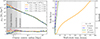 |
Fig. 1. Validation check of our super-sampled initial conditions. By stitching multiple runs of MUSIC, we created non-standard combinations of dark matter and gas mass zoom-in simulations. We ran five zoom-in simulations using the same initial conditions, increasing the dark matter mass resolution. We simulated each at a redshift of z = 1 and show the total matter density profile here in the left-hand panel with the relevant convergence radii in the grey regions (c.f. (6)). We find consistent density profiles over the range of mass resolutions. The right-hand panel shows the corresponding wall-clock time to simulate each halo at the same redshift. The colour and line-style match those in the left-hand panel, and we also show the final wall-clock time to simulate down to z = 1 in the legend. |
Interestingly, recent work has shown that a mismatch in particle mass (where often the dark matter mass is significantly larger than the stellar mass) in simulations can lead to numerical heating, artificially puffing up the halo (Ludlow et al. 2023, 2021; Revaz & Jablonka 2018). Here, we are in a different regime where the mean stellar mass is five times larger than the dark matter mass, potentially heating the dark matter and mimicking SIDM. We observe no such heating in the core of the clusters, potentially because the particle number of stars is so few that it would not have much impact. However, it is important to consider such an effect when super-sampling the ICs.
The final dark matter and initial gas mass resolution throughout the rest of this paper is mdm = 0.68 × 10⁸ M⊙ and mgas = 8.20 × 10⁸ M⊙, respectively (corresponding to level 10 and 12 in the MUSIC IC generator). We adopted a Plummer-equivalent comoving softening length of 8.93 ckpc, and a maximum smoothing length of 2.28 pkpc for both the baryons and the dark matter. Confident that the initial conditions (ICs) do not result in spurious numerical problems, we now look to calibrate our simulations.
2.3. Calibration
The special setup of our simulations, with super-sampled dark matter, requires us to recalibrate, since no hydro model has been tested in such an environment. Moreover, correctly calibrating the central brightest cluster galaxy is particularly important for SIDM, since the interplay between the inner regions of clusters and the stars can dramatically alter the resulting density profile (Robertson et al. 2018). For example, Harvey et al. (2019) found that the wobble BCG signal (a smoking gun of SIDM Kim et al. 2017) was extremely sensitive to the stellar content of the BCG. This makes logical sense, since the self-interactions are trying to expel particles, yet any large concentrations of stars will attempt to prevent this through gravitational drag and contraction effects coming from cooling of gas. As a result, we focused our calibration on the stellar fractions and size-mass relations of the BCGs, to ensure that we got accurate predictions of what SIDM does in the core of a cluster.
We calibrated our zooms equally to four key observables, including the gas mass fraction (Hoekstra et al. 2015), the stellar mass fraction (Golden-Marx et al. 2023; Kravtsov et al. 2018; Zhang et al. 2011; Akino et al. 2022), the BCG size-mass relation (Trujillo et al. 2020), and finally the stellar mass to halo mass function for BCGs (Gonzalez et al. 2013; Golden-Marx et al. 2023; DeMaio et al. 2020; Kravtsov et al. 2018; Huang et al. 2022). These are all equally important since obtaining the correct stellar fraction, as mentioned, is a focus of this project. We did not calibrate to our final sample of 100 massive clusters as this would take too long; hence, we chose a representative sample of 30 clusters equally spaced between 14 < log M200, crit/M⊙ < 15.5 in mass. These clusters span a large mass range for two reasons: the first is to ensure that we have a reasonable understanding of the mass dependence of our calibration decisions, and secondly, smaller mass halos are significantly faster to simulate and hence more efficient when tuning individual parameters. Although the simulations used to train the machine learning model in Kugel et al. (2023) have a slightly different feedback model to the one used here, the general principles remain, and hence we used this study to direct our calibration points, shifting the ΔTAGN and βBH to recreate realistic halos. We find for our sample the best fit hydro parameters are βBH = 0.5, ΔTAGN = 108 K. Finally, as in BAHAMAS, we chose to couple energy injections from AGN feedback to 20 nearest neighbours. We test a variety of numbers and find that the properties are not sensitive to this choice.
Following the calibration of the hydro parameters, we simulated the 100 most massive clusters in the initial 400 Mpc/h box. We show their mass distribution in Figure 2 and their final calibrated parameters in Figure 3. We also quantify the fit and scatter of our simulated clusters to ensure they are consistent with observations. The solid line in each case shows the best fit, and the regions show the 68% and 95% around this fit. We find our cluster matches extremely well the observations at this mass range. It is these clusters that will be re-simulated in a SIDM cosmology.
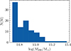 |
Fig. 2. Distribution of total mass (M200) of the 100 most massive galaxy clusters selected from the initial 400 Mpc/h box to be re-simulated. |
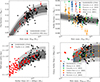 |
Fig. 3. Final calibrated set of DARKSKIES CDM clusters. In each panel, we show the zoom-in, super-sampled clusters with CDM in black stars. Specifically, top left: Gas fraction inside r500 as a function of the halo mass M500, top right: Stellar fraction inside r500 as a function of the halo mass M500, bottom left: Projected half-mass radius of the central galaxy (considering all stars inside 100 kpc) as a function of projected stellar mass within 100 kpc, bottom right: Projected stellar mass within 100 kpc as a function of halo mass. The Flamingo HST Data corresponds to a collection of gas mass estimates collated by the Flamingo team (Hoekstra et al. 2015; Eckert et al. 2016; Akino et al. 2022; Lin et al. 2012; Lovisari et al. 2015; Sun et al. 2009; Vikhlinin et al. 2006). The solid line in each case shows the best fit, and the regions show the 68% and 95% representing the one and two standard deviation confidence limits around this fit. |
2.4. SIDM parameter space
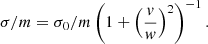
Optimally sampling the SIDM parameter space in order to provide a valuable dataset for a variety of scientific purposes is difficult. For example, when measuring classical parameters such as the offset between a central galaxy and the dark matter halo, a large sample of clusters simulated at the same cross-section is required in order to determine the overall distribution (Harvey et al. 2019). However, providing samples at many different cross-sections is often more valuable since it can provide more variable data for a model to fit to (e.g. Villaescusa-Navarro et al. 2021). Therefore, we must balance the two contrasting requirements since satisfying both is computationally unfeasible. We also note that should SIDM be velocity dependent, this introduces two new parameters (Robertson et al. 2018). However, as it was found in Robertson et al. (2019), halos at low redshift (z < 0.5) at a given mass (and hence characteristic particle velocity), simulated at a velocity-independent cross-section is qualitatively the same as if it was simulated with a velocity-dependent cross-section that had a matching parametrisation of the normalisation, σ0 and turn-over velocity, w, where the cross-section can be characterised, for a given dark matter model, as
 (5)
(5)
(see e.g. Robertson et al. 2019; Correa et al. 2022). In particular, machine learning algorithms cannot tell them apart (Harvey 2024). This idea of an ‘effective cross-section’ has been explored in Yang & Yu (2022) (in particular Eq. (4.2)). As such, we chose to simulate only velocity-independent cross-sections, since these can approximately be recast into velocity-dependent realisations (since the direct mapping is non-trivial). Note the caveat that the sub-halos do not correspond to the correct dark matter model, since with a velocity-dependent model we expect changes in the internal structure where particles move slower relative to one another (Palubski et al. 2024). Hence, any observables are valid only for the main halo, not sub-halos. Figure C.1 shows the effective models that we simulate here.
In order to identify halos across models and look-back time, we identified the main halo in each CDM, z = 0 snapshot and traced back the particle IDs for each simulation. This enabled us to carry out a like-for-like verification that the calibration is not dependent on the cross-section, and that in all cases the properties of the clusters do not change with respect to the cross-section and hence does not require a re-calibration. Finally, we identified five cross-sections to simulate, specifically chosen to align with the scientific goals of ‘DARKSKIES’. In order to achieve precision of σDM/m < 0.1 cm2/g, we required simulations that straddle this threshold. We therefore first selected a cross-section that targets optimistic constraints expected from future telescopes such as Euclid using machine learning (Harvey 2024) (σDM/m = 0.01 cm2/g), then a more conservative expectation at σDM/m = 0.05 cm2/g, the required limit of ‘DARKSKIES’ of σDM/m = 0.1 cm2/g (Harvey et al. 2017; Sirks et al. 2024) (and overlap with BAHAMAS-SIDM) and finally a larger cross-section at the current limit of what is observed σDM/m = 0.2 cm2/g, plus CDM (σDM/m = 0 cm2/g). We hereafter refer to these models as SIDM0.01, SIDM0.05, SIDM0.1, SIDM0.2, and CDM. A final overview of the simulations can be seen in Table 1.
Overview of the key simulation parameters.
3. Results
We now show the results from the simulations. We present an example cluster (ID = 20926) in Figure 4 for different redshifts (columns) and different dark matter models (rows). We observe the stochastic nature of the simulations means that although the structure of the halo is the same, the details vary from simulation to simulation. We next derive the 3D mass-density profiles for each set of clusters. In Figure 5, we show the median profile for each run and each mass component. In the main panel, we display the total density profile for each dark matter model simulated here in a solid line, with CDM in black, SIDM0.01 in orange, SIDM0.05 in purple, SIDM0.1 in blue, and SIDM0.2 in cyan. We also show the convergence radii with the vertical dotted line (Schaller et al. 2015b), where the convergence radii is defined as the smallest radius that satisfies
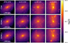 |
Fig. 4. Total mass density map for the halo 20926 at different redshifts (columns), simulated in different dark matter models (rows). Each panel has a field-of-view of 1 × 1 pMpc, has the same scaled colour bar, and has been projected along the z-axis of the simulation box. |
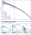 |
Fig. 5. Total (top panel), dark matter (bottom left panel), stellar (bottom middle panel), and gas (bottom right panel) mass density profiles as a function of self-interaction cross-section. In each case, we show the density relative to CDM, and in the main panel, we show the BAHAMAS SIDM simulations as dashed lines. In each case, the shaded region shows the 16% and 84% of the simulations. |
 (6)
(6)
where ρcrit is the critical density at the redshift of the cluster, mDM is the dark matter particle mass, and N is the number of particles. The original convergence radii ensured that the mean density within this radius has converged to within 10% of that of a higher resolution run (Power et al. 2003). However, (Schaller et al. 2015b) relaxed this assumption since baryons naturally add increased scatter, thus they chose a radius whereby the mean density within this radius has converged to within 20% of that of a higher resolution run. Theoretically, there should be no reason why this criterion should not hold here, and thus we adopt the same criterion here despite having different particle mass.
For comparison, we show the BAHAMAS+SIDM runs in dashed lines, with black showing CDM, blue showing SIDM0.1, red showing SIDM1, and velocity-dependent cross-section in green ( σ0/m = 3.04 cm2/g, w = 560 km/s or mχ = 0.15 GeV, mϕ = 0.28 keV and α = 6.74 × 10⁻⁶), which at these mass scales corresponds to an effective cross-section of ∼0.5 cm2/g. We show the convergence radii in the vertical dot-dashed line. Finally, we show in the bottom sub-panel the relative difference between each dark matter model and the DARKSKIES CDM run. We find that the BAHAMAS CDM runs agree extremely well with the CDM runs here.
In the bottom three panels of Figure 5, we show the 3D density profiles of the individual three mass components, including (from left to right) the dark matter density profile, the stellar density profile, and the gas profile, with the difference relative to CDM in the bottom sub-panel. The vertical dotted line shows the convergence radius for that mass component. We find that both the dark matter and stellar profiles are affected by the dark matter self-interactions, whereas the gas is not. However, because of the low resolution of the gas, it is difficult to make any firm conclusions from this plot.
We next examine the redshift dependence of the profile. Since scattering rates are linear in time, the signal should build up over cosmic time, with the largest differences at z = 0. Figure 6 shows the density profile with respect to CDM at different redshifts and look-back times tLB. We find that above a redshift of z = 0.5, the signal for SIDM all but disappears, with the largest differences at lower redshifts. However, there seems to be some suppression in the mass profile at intermediate radii for larger cross-sections (10 − 100 kpc, SIDM0.2), suggesting a difference in mass build-up of the cluster due to self-interactions. Interestingly, AIDA also finds tentative evidence of a difference in the halo mass function for SIDM models at high redshifts, suggesting that perhaps self-interactions are able to slow down the growth of structure.
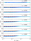 |
Fig. 6. Redshift dependence of the total matter 3D density profile of the clusters in the DARKSKIES simulations relative to the CDM case. Each panel shows the density profile for each SIDM model at a given redshift slice. The colours are the same as in Figure 5. |
Next we look at the offset between the dark matter halo and the BCG. Many studies have suggested that in a SIDM cosmology, any offset induced between the dark matter halo and BCG by a major merger at any point during the history of the cluster will persist, even long after the cluster has relaxed and virialised due to the flat potential in the core (Kim et al. 2017; Harvey et al. 2017, 2019). This offset is a feature of SIDM and not CDM. Since we cannot observe this ‘wobbling’ in real time, we can measure the one-point distribution of offsets between dark matter and the BCG and measure the median offset. The work in Harvey et al. (2017) identified the observable cosmological signal of the Wobble in 2D images of the cluster and how it scaled with the cross-section. However, it wasn’t clear whether this scaling was physically driven or as a result of increased error in a halo due to large dark matter cores. Here we want to identify very clearly, first the signal and its redshift dependence, and what processes are driving this.
To this end, we first have to carefully identify the centre of mass of each cluster. This is not sufficiently precise in the Velociraptor (VR) catalogues, and therefore we chose to re-find the centres of the halos. To do this, we first take the position as estimated by VR and then use shrinking spheres to find the centre of mass of both the BCG (assuming that the stars are the dominant mass baryonic component within the central region) and the dark matter. We begin at 50 kpc and incrementally shrink to 1 kpc (or when we run out of particles). We then measure the offset between the two estimators and take the median of the distribution (as has been done previously) for a given dark matter model and redshift. Fig. 7 shows the result with each panel showing the median offset as a function of cross-section for a given redshift (shown in the inset). To each figure, we fit a linear function (in log(σDM/m)), parametrised by,
 (7)
(7)
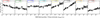 |
Fig. 7. Redshift evolution of the 3D median offset between the dark matter halo and the stellar halo for each model of dark matter from z = 2 (left) to z = 0 (right). We fit Eq. (7) to each snapshot and show the best fit with associated error in each panel. |
where a and b are free parameters to fit and the function inside the log takes the maximum value between the true cross-section and the effective cross-section due to coring by the artificial softening length of the simulation. Harvey et al. (2019) found that the effective cross-section for CDM was σeff ∼ 10−2 cm2/g, here the dark matter particle mass is almost two orders of magnitude smaller, resulting in a smoothing length ∼5 times smaller. We therefore chose an effective cross-section of σeff = 2 × 10⁻³ cm2/g. We find that altering this value does not substantially impact the fits in Figure 7. We study the evolution of a- the intercept (or the cross-section at σDM/m = 1.0 cm2/g) and b, the sensitivity of the wobble to the cross-section. The top panel of Figure 8 shows the time evolution of the intercept as a function of look-back time, tlb (and associated redshift on the top x-axis) and the middle panel shows the evolution of the wobble sensitivity. We find in both cases that they are very small at high redshift, with the sensitivity actually becoming negative. They both grow to peak around z = 0.25 (tlb = ∼3 Gyr); however, the wobble decreases afterwards, contrary to our expectation that the growth of cores would increase over time (Figure 6). Kim et al. (2017) showed that major mergers in cored halos drive the wobbles; therefore, we postulate that this wobble is driven by accretion of mass onto the halo. To understand this, we derive the mass accretion rate, which is simply the change in halo mass of each cluster with respect to time, and a proxy for the core size, which is the ratio of the 3D density at a radius of 10 kpc, ρ10 and at 100 kpc ρ100. We show the mass accretion (solid lines) and the density ratio (dotted lines) of each simulation in the bottom panel. We find that the mass accretion peaks at z ≃ 0.5, subsequently dropping off at lower redshifts. This is similar to other studies looking at merger rates of halos in simulations (Huško et al. 2022). We find that the shape of the mass accretion function is similar to that of both the wobble amplitude and the sensitivity albeit with a small delay. We hypothesise that this is because at z = 0.5 the core has not sufficiently grown yet for the wobble to persist. The dotted line supports this showing how the core does not become significant until z = 0.375. To estimate the lag, we fit a generalised model to the mean of the mass-accretion rate with a Gaussian process Regressor3 along with a Rational Quadratic kernel that has best fitting meta-parameters of scale-length, s = 100 and a α = 6.3. We show the corresponding fit as the dotted black line in the bottom panel of Figure 8. We hypothesise that it is this mass-accretion driving the relationship seen in the top two panels. We therefore adopt this shape and simply scale and stretch it such that we fit
 (8)
(8)
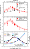 |
Fig. 8. Time evolution of the fits to Figure 7 parametrised by Eq. (7). The top panel shows the evolution of the intercept, a plus the absolute values of CDM and the evolving smooth length of the simulation. The middle panel shows the evolution of the gradient b as a function of look-back time (and respective redshift on the top axes). In both cases, the error bars of individual points come from the estimated error from scipy.curve_fit, and the shaded regions represent the 1 − σ error in rescaled fit of the mass accretion curve. To determine these, we performed Monte Carlo sampling of the fitted parameters around their uncertainties, drew random realisations of the fit, and found their 16% and 84%. The bottom panel shows the mean mass accretion for each model of dark matter as a function of look-back time. The thick dashed line is the best fitted model to the mean mass accretion, which is subsequently fitted to the top two panels by stretching in x and y (see Eq. (8)). The best fit is shown here in red (and the shaded region the 1σ error. We also calculated the shift between the peak of the mass accretion rate and the peak of the wobble. |
where g(x) is the normalised output of the Gaussian process fitted to the mass accretion, tLB is the look-back time, l is the lag, and d and e are values to be fitted. We fit to both the wobble amplitude and the sensitivity and show the resulting fit in the solid red and its 1 − σ error in the shaded region. We find in the case of the intercept (top panel of Figure 8) l = 1.7 ± 0.7 Gyr, d = 2.4 ± 0.6, e = 2.46 ± 0.34, and for the middle panel, l = 2.6 ± 0.6 Gyr, d = 1.4 ± 0.2, e = −0.5 ± 0.02, and in both cases, finding a remarkably good fit. The rapid drop-off in amplitude of the signal suggests that the timescale for dynamical relaxation is much smaller than the growth rate of the wobble driven by mass accretion.
We also look at the offsets in CDM (shown as clear circles in the top panel of Figure 8) and find that the offsets are not sensitive to mass accretion in the same way as SIDM for z < 0.75 and trace closely the softening length of the simulation. Moreover, interestingly, we find that the mass accretion in SIDM is lower at higher redshifts, leading to a negative dependence of the wobble on the cross-section. With lower redshift, the wobble traces the softening length of the simulation (dashed black line). This seems to be a combination of the decrease in mass accretion and that CDM experiences a lower density ratio at higher redshifts.
Given the coarse temporal resolution due to physical limitations of storage space for the snapshots, we chose to carry out one simulation with extremely high fidelity snapshots for two models (CDM and SIDM0.2) of dark matter to observe the connection between mass accretion and the dark matter wobble. We show the results in Figure 9. The first figure shows the mass accretion for the two models, showing that there is an order 1% difference between them. It also shows how there is a large amount of structure accreted at z ∼ 1.4, as well as at a later time at z ∼ 0.2. The second Figure shows the evolution of the offset between the dark matter and the BCG. We find that the offset for both models is consistent with each other until z < 0.5, when the SIDM0.2 model begins to exhibit oscillations at regular intervals with a peak amplitude of ∼10 kpc. To better show this, we overlay the median filter in a dotted line. The third figure shows the ratio between the 3D density at 10 kpc and 100 kpc, Γ = ρ10/ρ100. We see a similar trend to Figure 8, where at high redshifts SIDM0.2 seems to have a higher ratio, but as the halo evolves, we clearly see the creation of the core at z < 0.5. Finally, we cross-correlate the median-filtered offset with the mass accretion rate and show the result correlation,  as a function of the lag between the signals. We find that CDM exhibits no significant correlation between the two, and the peak correlation of SIDM0.2 lies at tlag = 1.2 Gyr, roughly consistent with that found for the overall distribution in Figure 8. Moreover, we find at early times that despite the large amount of accreted mass, neither dark matter model experiences any such oscillation. However, at late times, we find that now a core has been created, and the increase in mass accretion does instigate a wobbling. This supports the hypothesis that the wobble is driven by mass accretion in a cored halo.
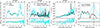 |
Fig. 9. High-fidelity simulation of a single halo for two dark matter models. The left-hand figure shows the mass accretion rate over cosmic time, with the bottom panel showing the accretion relative to CDM. The middle panel shows the evolution of the offset between the dark matter and the BCG, with a median filter (kernel size of 1 Gyr) shown by the dashed line. The oscillations and wobbles can be clearly seen at redshifts z < 0.5. The bottom panel of the middle figure shows the difference between the offsets, showing how the SIDM0.2 grows at late times. The final, right-hand figure shows the correlation between the mass accretion rate, Ṁ and the offset between the dark matter and the BCG (X) as a function of the time lag between the signals. We see that for this halo the peak correlation occurs at 1.3 Gyr, consistent with the over-distribution found in the bottom panel of Figure 8. |
Finally, to confirm the physical origin of the wobble (and not just increased error in the centring of the halo), we look at the velocity offset between the main halo and the stellar halo. Theoretically, should the BCG indeed wobble in the potential of the dark matter halo, the velocity should anti-correlate with the offset for SIDM and not for CDM. We explore this hypothesis and measure the relative velocity of the stars with respect to the centre of mass of the main halo (CoM). We then average this over all halos and all snapshots that have positive wobble (z < 0.75). In order to account for differing halo mass (since the acceleration is dependent on the mass of the main halo and not the stellar halo), we rescale the velocities by the inverse-square-root, i.e. 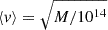 . Figure 10 shows the results for three of our dark matter models. We see clearly here that the anti-correlation is strongest with the highest cross-section and that CDM is consistent with no correlation. We fit a linear function to this relationship and show the gradient of this as an inset. We find the significance of the anti-correlation for SIDM0.2 is 10 standard deviations from the null hypothesis that there is no correlation. The intercept for the three plots are intCDM = 363 ± 21 km/s, intSIDM0.1 = 418 ± 14 km/s, intSIDM0.2 = 468 ± 16 km/s.
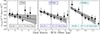 |
Fig. 10. Mean relative velocity of the BCG with respect to the main halo as a function of their 3D spatial offset for three of our dark matter models for all halos z < 0.75. We weight the velocities to the inverse square of the halo mass in order to stack. We show the wobble for each model with the vertical dashed line. A key signature of harmonic oscillation is the anti-correlation between the velocity and the distance. |
We note, however, that the velocities of the dark matter halo are not directly observable. It is possible that the intra cluster light (ICL) could trace this potential and therefore velocity estimates of the ICL could provide a way to trace its velocities. This is something for future work to look into.
4. Conclusions
We present a suite of one hundred zoom-in simulations of massive (M/M,200 > 5 × 10¹⁴) galaxy clusters simulated with five different self-interaction models including σDM/m = 0.,0.01, 0.05, 0.1, 0.2 cm2/g. We super-sampled our simulations reaching a dark matter / initial gas particle mass of mDM/mGas = ∼1/10 (whereas normally it is mDM/mGas ∼ 5). With this prescription and a dark matter particle mass of 0.68 × 10⁸ M⊙ we are able to probe previously untested cross-sections. We calibrated our simulations on four key observables: the gas fraction within R500, the stellar fraction within the same radius, the brightest cluster galaxy (BCG) half mass radius versus its total stellar mass, and the stellar mass to halo mass function of centrals. We are able to produce realistic galaxy clusters, and as in Robertson et al. (2019) we find that this calibration does not depend on the self-interaction cross-section and hence does not require re-calibration. We present our results and find that the predicted 3D density profiles predictably are less dense in the core of the cluster and converge to those of collisionless dark matter in the outskirts. We find that CDM matches extremely well, and we match the predictions from the BAHAMAS SIDM simulations down to the convergence radius of the simulations. We also find that even for the smallest cross-sections there is a discernible difference between the stellar and dark matter density profiles. We analysed the redshift dependence of the total matter density profile and find that the SIDM features only begin to reveal themselves in clusters at z < 0.5. Thus, any survey attempting to constrain SIDM should be limited to low redshift objects.
Following this we carried out an in-depth analysis of the cosmological ‘wobbling’ signal, whereby the BCG oscillates in the bottom of an SIDM cored dark matter potential. We find that counter to expectations the 3D wobbling signal peaks at z = 0.25, dropping thereafter, despite the core size continuing to increase. We measured the mass accretion rate of the halos in each cosmology and the core creation time and find that the wobble traces this rate remarkably well, albeit with a delay due to the late time creation of the dark matter core (that is required for the BCG to wobble). Interestingly, we find that SIDM0.2 has a delayed mass accretion. We find that the wobble amplitude falls off extremely quickly at late times when mass accretion also drops, suggesting that these oscillations have relatively short relaxation times. We measured the lag between the mass accretion and the formation of a wobble to be tlag = 2.6 ± 0.6 Gyr. We followed this up by measuring the correlation between the separation of the BCG and the dark matter halo and the relative velocity of the two halos – a hallmark of harmonic oscillation. We find that SIDM0.2 exhibits an extremely strong anti-correlation, whereas CDM seems to have no such anti-correlation, once again supporting the existence of a physical oscillation of the BCG in SIDM cosmologies. This is encouraging, as any observed offset between dark matter and the BCG (in any halo) is likely an unambiguous signal of SIDM.
With the expected arrival of all-sky surveys such as Euclid in the coming year, we will require robust predictions for possible dark matter models. Self-interacting dark matter is theoretically robust and empirically possible, and as such represents an ideal candidate for dark matter. However, if we are to exploit the forthcoming data, we require theoretical predictions to match. This suite of simulations represents a pathway to delivering high-resolution particle dark matter simulations at a fraction of the CPU cost. By super-sampling the dark sector, we can resolve faint scatterings and make robust predictions. Moreover, by simulating many more points in the dark matter parameter space, we provide further data to train, test, and validate our models. In order to facilitate the usefulness of these simulations, we make them freely available and public to the community.
Data availability
Postage stamps of all models are available at https://drive.google.com/file/d/1ib8btBb0iZ35wDw_HW70W2oeyQ6pIvTQ/view?usp=share_link. These data consist of 2D maps, binned to 20 kpc in resolutions out to 2 Mpc (resulting in image dimensions of 100 × 100). We provide total mass maps, dark matter, X-ray emission maps, and stellar distributions, resulting in 4 channels. These are projected in three axes resulting in a final shape of (300 × 4 × 100 × 100). We provide snapshots 10, 9, 8, and 7, (z = 0.000, z = 0.125, z = 0.250, and z = 0.375) and for all SIDM models. For full particle data and catalogues please contact corresponding author.
A term that includes all known processes associated with galaxy formation.
Constraints using cluster sphericity had previously been reported. However, subsequent simulations showed that observations were consistent with simulations (Miralda-Escudé 2002; Meneghetti et al. 2001).
Acknowledgments
This work was supported by the Swiss State Secretariat for Education, Research and Innovation (SERI) under contract number 521107294. This work was supported by a grant from the Swiss National Supercomputing Centre (CSCS) under project ID s1235 on Alps. The authors would like to thank Camila Correa without whom this project would not have got off the ground and John Biddiscombe for providing valuable insights and aid with the HPC at CSCS.
References
- Abbott, T. M. C., Abdalla, F. B., Alarcon, A., et al. 2018, Phys. Rev. D, 98, 043526 [NASA ADS] [CrossRef] [Google Scholar]
- Akino, D., Eckert, D., Okabe, N., et al. 2022, PASJ, 74, 175 [NASA ADS] [CrossRef] [Google Scholar]
- Angulo, R. E., & Hahn, O. 2022, Liv. Rev. Comput. Astrophys., 8, 1 [CrossRef] [Google Scholar]
- Bahé, Y. M., Schaye, J., Schaller, M., et al. 2022, MNRAS, 516, 167 [CrossRef] [Google Scholar]
- Balberg, S., Shapiro, S. L., & Inagaki, S. 2002, ApJ, 568, 475 [CrossRef] [Google Scholar]
- Barnes, D. J., Kay, S. T., Bahé, Y. M., et al. 2017, MNRAS, 471, 1088 [Google Scholar]
- Bartelmann, M., & Schneider, P. 2001, Phys. Rep., 340, 291 [Google Scholar]
- Bennett, C. L., Larson, D., Weiland, J. L., et al. 2013, ApJS, 208, 20 [Google Scholar]
- Booth, C. M., & Schaye, J. 2009, MNRAS, 398, 53 [Google Scholar]
- Borrow, J., Schaller, M., Bahé, Y. M., et al. 2023, MNRAS, 526, 2441 [Google Scholar]
- Boylan-Kolchin, M., Bullock, J. S., & Kaplinghat, M. 2011, MNRAS, 415, L40 [NASA ADS] [CrossRef] [Google Scholar]
- Bradač, M., Allen, S. W., Treu, T., et al. 2008, ApJ, 687, 959 [CrossRef] [Google Scholar]
- Brooks, A. M., Kuhlen, M., Zolotov, A., & Hooper, D. 2013, ApJ, 765, 22 [NASA ADS] [CrossRef] [Google Scholar]
- Buckley, M. R., Zavala, J., Cyr-Racine, F.-Y., Sigurdson, K., & Vogelsberger, M. 2014, Phys. Rev. D, 90, 043524 [Google Scholar]
- Cardona-Barrero, S., Battaglia, G., Nipoti, C., & Di Cintio, A. 2023, MNRAS, 522, 3058 [CrossRef] [Google Scholar]
- Chabrier, G. 2003, PASP, 115, 763 [Google Scholar]
- Chaikin, E., Schaye, J., Schaller, M., et al. 2022, MNRAS, 514, 249 [Google Scholar]
- Clowe, D., Bradač, M., Gonzalez, A. H., et al. 2006, ApJ, 648, L109 [NASA ADS] [CrossRef] [Google Scholar]
- Correa, C. A. 2021, MNRAS, 503, 920 [NASA ADS] [CrossRef] [Google Scholar]
- Correa, C. A., Schaller, M., Ploeckinger, S., et al. 2022, MNRAS, 517, 3045 [NASA ADS] [CrossRef] [Google Scholar]
- Correa, C. A., Schaller, M., Schaye, J., et al. 2025, MNRAS, 536, 3338 [Google Scholar]
- Dalla Vecchia, C., & Schaye, J. 2012, MNRAS, 426, 140 [NASA ADS] [CrossRef] [Google Scholar]
- Davis, M., Lecar, M., Pryor, C., & Witten, E. 1981, ApJ, 250, 423 [Google Scholar]
- Davis, M., Efstathiou, G., Frenk, C. S., & White, S. D. M. 1985, ApJ, 292, 371 [Google Scholar]
- de Blok, W. J. G. 2010, Adv. Astron., 2010, 5 [Google Scholar]
- DeMaio, T., Gonzalez, A. H., Zabludoff, A., et al. 2020, MNRAS, 491, 3751 [Google Scholar]
- Despali, G., Heinze, F. M., Fassnacht, C. D., et al. 2025a, A&A, 699, A222 [NASA ADS] [CrossRef] [EDP Sciences] [Google Scholar]
- Despali, G., Moscardini, L., Nelson, D., et al. 2025b, A&A, 697, A213 [NASA ADS] [CrossRef] [EDP Sciences] [Google Scholar]
- Dolag, K. 2015, IAU Gen. Assembly, 29, 2250156 [Google Scholar]
- Dubinski, J., & Carlberg, R. G. 1991, ApJ, 378, 496 [Google Scholar]
- Eckert, D., Ettori, S., Coupon, J., et al. 2016, A&A, 592, A12 [NASA ADS] [CrossRef] [EDP Sciences] [Google Scholar]
- Elahi, P. J., Cañas, R., Poulton, R. J. J., et al. 2019, Pasa, 36, e021 [Google Scholar]
- Ferland, G. 2017, Plasma simulations that meet the challenges of HST& JWST Active Nuclei& Starburst observations. HST Proposal id.15018. Cycle 25 [Google Scholar]
- Golden-Marx, J. B., Zhang, Y., Ogando, R. L. C., et al. 2023, MNRAS, 521, 478 [Google Scholar]
- Gonzalez, A. H., Sivanandam, S., Zabludoff, A. I., & Zaritsky, D. 2013, ApJ, 778, 14 [Google Scholar]
- Hahn, O., & Abel, T. 2011, MNRAS, 415, 2101 [Google Scholar]
- Harvey, D. 2024, Nat. Astron., 8, 1332 [Google Scholar]
- Harvey, D., Massey, R., Kitching, T., Taylor, A., & Tittley, E. 2015, Science, 347, 1462 [Google Scholar]
- Harvey, D., Courbin, F., Kneib, J. P., & McCarthy, I. G. 2017, MNRAS, 472, 1972 [CrossRef] [Google Scholar]
- Harvey, D., Revaz, Y., Robertson, A., & Hausammann, L. 2018, MNRAS, 481, L89 [NASA ADS] [CrossRef] [Google Scholar]
- Harvey, D., Robertson, A., Massey, R., & McCarthy, I. G. 2019, MNRAS, 488, 1572 [NASA ADS] [CrossRef] [Google Scholar]
- Hildebrandt, H., Viola, M., Heymans, C., et al. 2017, MNRAS, 465, 1454 [Google Scholar]
- Hoekstra, H., Herbonnet, R., Muzzin, A., et al. 2015, MNRAS, 449, 685 [NASA ADS] [CrossRef] [Google Scholar]
- Huang, S., Leauthaud, A., Bradshaw, C., et al. 2022, MNRAS, 515, 4722 [NASA ADS] [CrossRef] [Google Scholar]
- Huško, F., Lacey, C. G., & Baugh, C. M. 2022, MNRAS, 509, 5918 [Google Scholar]
- Kamada, A., Kaplinghat, M., Pace, A. B., & Yu, H.-B. 2017, Phys. Rev. Lett., 119, 111102 [Google Scholar]
- Kaplinghat, M., Valli, M., & Yu, H.-B. 2019, MNRAS, 490, 231 [NASA ADS] [CrossRef] [Google Scholar]
- Kauffmann, G., White, S. D. M., & Guiderdoni, B. 1993, MNRAS, 264, 201 [Google Scholar]
- Kim, S. Y., Peter, A. H. G., & Wittman, D. 2017, MNRAS, 469, 1414 [NASA ADS] [CrossRef] [Google Scholar]
- Klypin, A., Kravtsov, A. V., Valenzuela, O., & Prada, F. 1999, ApJ, 522, 82 [Google Scholar]
- Koda, J., & Shapiro, P. R. 2011, MNRAS, 415, 1125 [NASA ADS] [CrossRef] [Google Scholar]
- Kravtsov, A. V., Vikhlinin, A. A., & Meshcheryakov, A. V. 2018, Astron. Lett., 44, 8 [Google Scholar]
- Kugel, R., Schaye, J., Schaller, M., et al. 2023, MNRAS, 526, 6103 [NASA ADS] [CrossRef] [Google Scholar]
- Li, S., Li, R., Wang, K., et al. 2025, arXiv e-prints [arXiv:2504.11800] [Google Scholar]
- Lin, Y.-T., Stanford, S. A., Eisenhardt, P. R. M., et al. 2012, ApJ, 745, L3 [Google Scholar]
- Lovisari, L., Reiprich, T. H., & Schellenberger, G. 2015, A&A, 573, A118 [NASA ADS] [CrossRef] [EDP Sciences] [Google Scholar]
- Ludlow, A. D., Fall, S. M., Schaye, J., & Obreschkow, D. 2021, MNRAS, 508, 5114 [NASA ADS] [CrossRef] [Google Scholar]
- Ludlow, A. D., Fall, S. M., Wilkinson, M. J., Schaye, J., & Obreschkow, D. 2023, MNRAS, 525, 5614 [NASA ADS] [CrossRef] [Google Scholar]
- Markevitch, M., Gonzalez, A. H., Clowe, D., et al. 2004, ApJ, 606, 819 [NASA ADS] [CrossRef] [Google Scholar]
- Mateo, M. L. 1998, ARA&A, 36, 435 [NASA ADS] [CrossRef] [Google Scholar]
- McCarthy, I. G., Schaye, J., Bird, S., & Le Brun, A. M. C. 2017, MNRAS, 465, 2936 [Google Scholar]
- McCarthy, I. G., Bird, S., Schaye, J., et al. 2018, MNRAS, 476, 2999 [NASA ADS] [CrossRef] [Google Scholar]
- Meneghetti, M., Yoshida, N., Bartelmann, M., et al. 2001, MNRAS, 325, 435 [NASA ADS] [CrossRef] [Google Scholar]
- Merten, J., Coe, D., Dupke, R., et al. 2011, MNRAS, 417, 333 [NASA ADS] [CrossRef] [Google Scholar]
- Miralda-Escudé, J. 2002, ApJ, 564, 60 [NASA ADS] [CrossRef] [Google Scholar]
- Moore, B., Ghigna, S., Governato, F., et al. 1999, ApJ, 524, L19 [Google Scholar]
- Nadler, E. O., Yang, D., & Yu, H.-B. 2023, ApJ, 958, L39 [NASA ADS] [CrossRef] [Google Scholar]
- Nadler, E. O., Kong, D., Yang, D., & Yu, H.-B. 2025, ApJ, 991, 69 [Google Scholar]
- Nelson, D., Pillepich, A., Springel, V., et al. 2018, MNRAS, 475, 624 [Google Scholar]
- Oman, K. A., Navarro, J. F., Fattahi, A., et al. 2015, MNRAS, 452, 3650 [CrossRef] [Google Scholar]
- Palubski, I., Slone, O., Kaplinghat, M., Lisanti, M., & Jiang, F. 2024, JCAP, 2024, 074 [Google Scholar]
- Peter, A. H. G., Rocha, M., Bullock, J. S., & Kaplinghat, M. 2013, MNRAS, 430, 105 [Google Scholar]
- Planck Collaboration VI. 2020, A&A, 641, A6 [NASA ADS] [CrossRef] [EDP Sciences] [Google Scholar]
- Ploeckinger, S., & Schaye, J. 2020, MNRAS, 497, 4857 [CrossRef] [Google Scholar]
- Pontzen, A., & Governato, F. 2014, Nature, 506, 171 [NASA ADS] [CrossRef] [Google Scholar]
- Power, C., Navarro, J. F., Jenkins, A., et al. 2003, MNRAS, 338, 14 [Google Scholar]
- Ragagnin, A., Meneghetti, M., Calura, F., et al. 2024, A&A, 687, A270 [NASA ADS] [CrossRef] [EDP Sciences] [Google Scholar]
- Randall, S. W., Markevitch, M., Clowe, D., Gonzalez, A. H., & Bradač, M. 2008, ApJ, 679, 1173 [NASA ADS] [CrossRef] [Google Scholar]
- Revaz, Y., & Jablonka, P. 2018, A&A, 616, A96 [NASA ADS] [CrossRef] [EDP Sciences] [Google Scholar]
- Robertson, A., Massey, R., Eke, V., et al. 2018, MNRAS, 476, L20 [Google Scholar]
- Robertson, A., Harvey, D., Massey, R., et al. 2019, MNRAS, 488, 3646 [NASA ADS] [CrossRef] [Google Scholar]
- Robles, V. H., Bullock, J. S., Elbert, O. D., et al. 2017, MNRAS, 472, 2945 [NASA ADS] [CrossRef] [Google Scholar]
- Rocha, M., Peter, A. H. G., Bullock, J. S., et al. 2013, MNRAS, 430, 81 [NASA ADS] [CrossRef] [Google Scholar]
- Roche, C., McDonald, M., Borrow, J., et al. 2024, Open J. Astrophys., 7, 65 [Google Scholar]
- Rubin, V. C., Ford, W. K. J., & Thonnard, N. 1980, ApJ, 238, 471 [NASA ADS] [CrossRef] [Google Scholar]
- Sagunski, L., Gad-Nasr, S., Colquhoun, B., Robertson, A., & Tulin, S. 2021, JCAP, 2021, 024 [CrossRef] [Google Scholar]
- Schaller, M., Robertson, A., Massey, R., Bower, R. G., & Eke, V. R. 2015a, MNRAS, 453, L58 [Google Scholar]
- Schaller, M., Frenk, C. S., Bower, R. G., et al. 2015b, MNRAS, 451, 1247 [Google Scholar]
- Schaller, M., Borrow, J., Draper, P. W., et al. 2024, MNRAS, 530, 2378 [NASA ADS] [CrossRef] [Google Scholar]
- Schaye, J., & Dalla Vecchia, C. 2008, MNRAS, 383, 1210 [Google Scholar]
- Schaye, J., Dalla Vecchia, C., Booth, C. M., et al. 2010, MNRAS, 402, 1536 [Google Scholar]
- Schaye, J., Crain, R. A., Bower, R. G., et al. 2015, MNRAS, 446, 521 [Google Scholar]
- Schaye, J., Kugel, R., Schaller, M., et al. 2023, MNRAS, 526, 4978 [NASA ADS] [CrossRef] [Google Scholar]
- Sirks, E. L., Harvey, D., Massey, R., et al. 2024, MNRAS, 530, 3160 [Google Scholar]
- Springel, V. 2005, MNRAS, 364, 1105 [Google Scholar]
- Springel, V., White, S. D. M., Jenkins, A., et al. 2005, Nature, 435, 629 [Google Scholar]
- Springel, V., Frenk, C. S., & White, S. D. M. 2006, Nature, 440, 1137 [NASA ADS] [CrossRef] [Google Scholar]
- Sun, M., Voit, G. M., Donahue, M., et al. 2009, ApJ, 693, 1142 [NASA ADS] [CrossRef] [Google Scholar]
- Trujillo, I., Chamba, N., & Knapen, J. H. 2020, MNRAS, 493, 87 [NASA ADS] [CrossRef] [Google Scholar]
- Vikhlinin, A., Kravtsov, A., Forman, W., et al. 2006, ApJ, 640, 691 [Google Scholar]
- Villaescusa-Navarro, F., Anglés-Alcázar, D., Genel, S., et al. 2021, ApJ, 915, 71 [NASA ADS] [CrossRef] [Google Scholar]
- Williams, L. L. R., & Saha, P. 2011, MNRAS, 415, 448 [Google Scholar]
- Yang, D., & Yu, H.-B. 2022, JCAP, 2022, 077 [CrossRef] [Google Scholar]
- Zhang, Y. Y., Laganá, T. F., Pierini, D., et al. 2011, A&A, 535, A78 [NASA ADS] [CrossRef] [EDP Sciences] [Google Scholar]
- Zwicky, F. 1933, Helv. Phys. Acta, 6, 110 [NASA ADS] [Google Scholar]
Appendix A: Further convergence tests
We carried out further convergence tests to ensure that our simulations do not suffer from any numerical artefacts. We simulate the same halo four times with the same resolution levels as in Figure 1. We label each simulation according to their MUSIC initial conditions level, with the first number referring to the baryonic / initial gas mass resolution and the second the dark matter particle resolution. For these convergence tests we output many more snapshots in order to get a high-fidelity view of the growth of our halos. We analyse four key properties from the output including: mass accretion rate (left hand panels of figure A.1), the stellar mass growth of the central halo (i.e. the star formation rate) in the middle panels of figure A.1, and the dark matter - brightest cluster offset for each resolution over the entire cosmic time. The final test is the consistency of sub-halo mass function. Figure A.2 shows the mass function for sub-halos inside one virial radii of the cluster. We find that the sub-halo mass functions for the target resolution is moderately suppressed below M200 < 2 × 10¹⁰ M⊙. It is difficult to interpret whether this is due to the super-sampling, or due to the halo-finder struggling to identify halos with significantly different particle masses. We found that chosen parameters for the VELOciraptor halo finder resulted in a broad range of predicted mass functions for the target resolution. Despite the moderate suppression, halos of this mass will not affect the results of this work, which focuses on the main halo properties. Future work studying sub-halos in super-sampled SIDM should consider looking in to this further.
We notice that the dark matter - brightest cluster galaxy offsets can sometimes be very noisy with offsets greater than 20 kpc observed. These outliers occur either in low resolution simulations where halos are hard to separate, or at times of very high mass accretion at early times when halo separation is again difficult. Indeed, our target resolution does not suffer from these outliers. We therefore conclude that our simulations do not appear to suffer from any artefacts due to super-sampling of the dark matter.
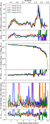 |
Fig. A.1. Additional convergence tests. Each panel shows results from the same halo for four different resolutions as found in Figure 1, where the first number corresponds to the level used in MUSIC for the gas mass, and the second for the dark matter. Each figure shows the absolute value in the top panel and the value relative to the high resolution, level 12-12, simulation in the bottom panel. From left to right, we show the mass accretion rate, the stellar mass within 100kpc, and the dark matter - brightest cluster galaxy offset. As expected we find no clear difference between the different runs in all cases. |
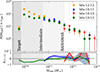 |
Fig. A.2. Consistency of the sub-halo mass function. We count the number of mass halos inside one virial radii of the cluster and show their mass distribution here. Assuming a minimum particle number of 100 particles for a halo, we show the mass resolution limit of each simulation where BAHAMAS is roughly equal to levels 10-10, intermediate corresponds to levels 10-11, and target corresponds to levels 10-12. The bottom panel shows the ratio between the mass function and the highest resolution, non-super-sampled run (12-12). We find that the sub-halo mass functions for the target resolution is moderately suppressed below M200 < 2 × 10¹⁰ M⊙. |
Appendix B: Contamination from boundary particles
Boundary particles exist in the simulation to trace the large-scale tidal fields that impact the growth of structure in the high-resolution regime. These particles theoretically should never actually enter this regime. However, when the initial Lagrangian region from which the initial conditions is cut, is too small, contamination can occur. In order to understand the contamination in our high-resolution we identify the boundary particles within the high-resolution region at z = 0. We estimate the contamination by boundary particles and in Figure B.1 show this a function of cluster centric radii (expecting increase in contamination as you tend to the boundary edge), where we define the contamination, c as:
 (B.1)
(B.1)
where nb and nd are the number of boundary and dark matter particles, respectively.
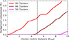 |
Fig. B.1. Boundary particles, or low resolution particles tracing the large-scale structure. These should not enter the high-resolution region; however, in rare cases this may occur. We show here the level of contamination (B.1), in the main halo of boundary particles as a function of radius from the centre of the halo. Each line shows the maximum contamination for a given number of halos. Thus, for example, half of the halos have negligible contamination (orange line), with 95% of our clusters having less than 2% contamination at 5 virial radii (dark red line). |
Appendix C: Effective velocity-dependent models
Simulating velocity-independent models, is qualitatively the same at simulating velocity-dependent models, for a given halo mass and redshift. We show here the effective models we simulate here ( for a given halo mass at a z = 0 ), assuming that relative particle velocities follow  . The stars show the velocity-dependent models, and the lines show how these can be recast into velocity-dependent models, assuming a constant asymptotic cross-section (top panel) or a constant turn over velocity (bottom panel). The caveat here is that the sub-halos remain unchanged in these models, whereas in a true velocity- dependent model, the lower particle velocities in these halos would change their mass distribution slightly.
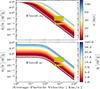 |
Fig. C.1. Effective models simulated ( for a given halo mass at a z = 0 ), assuming relative particle velocities following |

All Tables
All Figures
|
Fig. 1. Validation check of our super-sampled initial conditions. By stitching multiple runs of MUSIC, we created non-standard combinations of dark matter and gas mass zoom-in simulations. We ran five zoom-in simulations using the same initial conditions, increasing the dark matter mass resolution. We simulated each at a redshift of z = 1 and show the total matter density profile here in the left-hand panel with the relevant convergence radii in the grey regions (c.f. (6)). We find consistent density profiles over the range of mass resolutions. The right-hand panel shows the corresponding wall-clock time to simulate each halo at the same redshift. The colour and line-style match those in the left-hand panel, and we also show the final wall-clock time to simulate down to z = 1 in the legend. |
| In the text | |
|
Fig. 2. Distribution of total mass (M200) of the 100 most massive galaxy clusters selected from the initial 400 Mpc/h box to be re-simulated. |
| In the text | |
|
Fig. 3. Final calibrated set of DARKSKIES CDM clusters. In each panel, we show the zoom-in, super-sampled clusters with CDM in black stars. Specifically, top left: Gas fraction inside r500 as a function of the halo mass M500, top right: Stellar fraction inside r500 as a function of the halo mass M500, bottom left: Projected half-mass radius of the central galaxy (considering all stars inside 100 kpc) as a function of projected stellar mass within 100 kpc, bottom right: Projected stellar mass within 100 kpc as a function of halo mass. The Flamingo HST Data corresponds to a collection of gas mass estimates collated by the Flamingo team (Hoekstra et al. 2015; Eckert et al. 2016; Akino et al. 2022; Lin et al. 2012; Lovisari et al. 2015; Sun et al. 2009; Vikhlinin et al. 2006). The solid line in each case shows the best fit, and the regions show the 68% and 95% representing the one and two standard deviation confidence limits around this fit. |
| In the text | |
|
Fig. 4. Total mass density map for the halo 20926 at different redshifts (columns), simulated in different dark matter models (rows). Each panel has a field-of-view of 1 × 1 pMpc, has the same scaled colour bar, and has been projected along the z-axis of the simulation box. |
| In the text | |
|
Fig. 5. Total (top panel), dark matter (bottom left panel), stellar (bottom middle panel), and gas (bottom right panel) mass density profiles as a function of self-interaction cross-section. In each case, we show the density relative to CDM, and in the main panel, we show the BAHAMAS SIDM simulations as dashed lines. In each case, the shaded region shows the 16% and 84% of the simulations. |
| In the text | |
|
Fig. 6. Redshift dependence of the total matter 3D density profile of the clusters in the DARKSKIES simulations relative to the CDM case. Each panel shows the density profile for each SIDM model at a given redshift slice. The colours are the same as in Figure 5. |
| In the text | |
|
Fig. 7. Redshift evolution of the 3D median offset between the dark matter halo and the stellar halo for each model of dark matter from z = 2 (left) to z = 0 (right). We fit Eq. (7) to each snapshot and show the best fit with associated error in each panel. |
| In the text | |
|
Fig. 8. Time evolution of the fits to Figure 7 parametrised by Eq. (7). The top panel shows the evolution of the intercept, a plus the absolute values of CDM and the evolving smooth length of the simulation. The middle panel shows the evolution of the gradient b as a function of look-back time (and respective redshift on the top axes). In both cases, the error bars of individual points come from the estimated error from scipy.curve_fit, and the shaded regions represent the 1 − σ error in rescaled fit of the mass accretion curve. To determine these, we performed Monte Carlo sampling of the fitted parameters around their uncertainties, drew random realisations of the fit, and found their 16% and 84%. The bottom panel shows the mean mass accretion for each model of dark matter as a function of look-back time. The thick dashed line is the best fitted model to the mean mass accretion, which is subsequently fitted to the top two panels by stretching in x and y (see Eq. (8)). The best fit is shown here in red (and the shaded region the 1σ error. We also calculated the shift between the peak of the mass accretion rate and the peak of the wobble. |
| In the text | |
|
Fig. 9. High-fidelity simulation of a single halo for two dark matter models. The left-hand figure shows the mass accretion rate over cosmic time, with the bottom panel showing the accretion relative to CDM. The middle panel shows the evolution of the offset between the dark matter and the BCG, with a median filter (kernel size of 1 Gyr) shown by the dashed line. The oscillations and wobbles can be clearly seen at redshifts z < 0.5. The bottom panel of the middle figure shows the difference between the offsets, showing how the SIDM0.2 grows at late times. The final, right-hand figure shows the correlation between the mass accretion rate, Ṁ and the offset between the dark matter and the BCG (X) as a function of the time lag between the signals. We see that for this halo the peak correlation occurs at 1.3 Gyr, consistent with the over-distribution found in the bottom panel of Figure 8. |
| In the text | |
|
Fig. 10. Mean relative velocity of the BCG with respect to the main halo as a function of their 3D spatial offset for three of our dark matter models for all halos z < 0.75. We weight the velocities to the inverse square of the halo mass in order to stack. We show the wobble for each model with the vertical dashed line. A key signature of harmonic oscillation is the anti-correlation between the velocity and the distance. |
| In the text | |
|
Fig. A.1. Additional convergence tests. Each panel shows results from the same halo for four different resolutions as found in Figure 1, where the first number corresponds to the level used in MUSIC for the gas mass, and the second for the dark matter. Each figure shows the absolute value in the top panel and the value relative to the high resolution, level 12-12, simulation in the bottom panel. From left to right, we show the mass accretion rate, the stellar mass within 100kpc, and the dark matter - brightest cluster galaxy offset. As expected we find no clear difference between the different runs in all cases. |
| In the text | |
|
Fig. A.2. Consistency of the sub-halo mass function. We count the number of mass halos inside one virial radii of the cluster and show their mass distribution here. Assuming a minimum particle number of 100 particles for a halo, we show the mass resolution limit of each simulation where BAHAMAS is roughly equal to levels 10-10, intermediate corresponds to levels 10-11, and target corresponds to levels 10-12. The bottom panel shows the ratio between the mass function and the highest resolution, non-super-sampled run (12-12). We find that the sub-halo mass functions for the target resolution is moderately suppressed below M200 < 2 × 10¹⁰ M⊙. |
| In the text | |
|
Fig. B.1. Boundary particles, or low resolution particles tracing the large-scale structure. These should not enter the high-resolution region; however, in rare cases this may occur. We show here the level of contamination (B.1), in the main halo of boundary particles as a function of radius from the centre of the halo. Each line shows the maximum contamination for a given number of halos. Thus, for example, half of the halos have negligible contamination (orange line), with 95% of our clusters having less than 2% contamination at 5 virial radii (dark red line). |
| In the text | |
|
Fig. C.1. Effective models simulated ( for a given halo mass at a z = 0 ), assuming relative particle velocities following |
| In the text | |
Current usage metrics show cumulative count of Article Views (full-text article views including HTML views, PDF and ePub downloads, according to the available data) and Abstracts Views on Vision4Press platform.
Data correspond to usage on the plateform after 2015. The current usage metrics is available 48-96 hours after online publication and is updated daily on week days.
Initial download of the metrics may take a while.