| Issue |
A&A
Volume 703, November 2025
|
|
|---|---|---|
| Article Number | A138 | |
| Number of page(s) | 10 | |
| Section | Cosmology (including clusters of galaxies) | |
| DOI | https://doi.org/10.1051/0004-6361/202555389 | |
| Published online | 13 November 2025 | |
The origin of the JWST supermassive black holes
1
Keemilise ja Bioloogilise Füüsika Instituut, Rävala pst. 10, 10143 Tallinn, Estonia
2
Department of Cybernetics, Tallinn University of Technology, Akadeemia tee 21, 12618 Tallinn, Estonia
3
King’s College London, Strand, London WC2R 2LS, United Kingdom
4
Theoretical Physics Department, CERN, Geneva, Switzerland
5
Dipartimento di Fisica e Astronomia, Università degli Studi di Padova, Via Marzolo 8, 35131 Padova, Italy
6
Istituto Nazionale di Fisica Nucleare, Sezione di Padova, Via Marzolo 8, 35131 Padova, Italy
⋆ Corresponding author: This email address is being protected from spambots. You need JavaScript enabled to view it.
Received:
5
May
2025
Accepted:
6
August
2025
Abstract
We present a new semi-analytical model for the evolution of galaxies and supermassive black holes (SMBHs) that is based on the extended Press-Schechter formalism and phenomenological modelling of star formation. The model yields black-hole-mass – stellar mass relations that reproduce both the JWST and pre-JWST observations. If the efficiency for BH mergers is high, the JWST data prefer light seeds, while the pre-JWST data prefer heavy seeds. The fit improves for a smaller merger efficiency, 𝒪(0.1), for which both data prefer heavy seeds, while also accommodating the pulsar-timing-array gravitational-wave background data.
Key words: cosmology: theory
© The Authors 2025
 Open Access article, published by EDP Sciences, under the terms of the Creative Commons Attribution License (https://creativecommons.org/licenses/by/4.0), which permits unrestricted use, distribution, and reproduction in any medium, provided the original work is properly cited.
This article is published in open access under the Subscribe to Open model. This email address is being protected from spambots. You need JavaScript enabled to view it. to support open access publication.
1. Introduction
The origin of supermassive black holes (SMBHs) is (literally) one of the biggest problems in astrophysics and cosmology (Volonteri et al. 2021). It has been thrown into the limelight recently by two sets of observations: the discovery of a (surprisingly strong) stochastic background of nanoHertz gravitational waves (GWs) by pulsar timing arrays (PTAs) (Agazie et al. 2023a; EPTA Collaboration and InPTA Collaboration 2024; Reardon et al. 2023; Xu et al. 2023) and the discovery of a (surprisingly heavy) population of SMBHs at high redshifts, z ≳ 4 by the JWST (Übler et al. 2023; Larson et al. 2023; Harikane et al. 2023a; Bogdan et al. 2024; Ding et al. 2023; Maiolino et al. 2024; Yue et al. 2024; Kocevski et al. 2023; Stone et al. 2024). The PTA signal is commonly thought to have been emitted by SMBH binary systems and points towards relatively high SMBH merger efficiency (EPTA Collaboration and InPTA Collaboration 2023; Agazie et al. 2023b; Ellis et al. 2024a,b; Bi et al. 2023; Raidal et al. 2024), although fundamental physics sources are also allowed by the available data (EPTA Collaboration and InPTA Collaboration 2024; Figueroa et al. 2024; Afzal et al. 2023; Ellis et al. 2024c). It has been suggested that the JWST observations may indicate a bias in either the high-z or local active galactic nuclei (AGN) observations (Li et al. 2025; Ellis et al. 2024b) and a preference for heavy SMBH seed scenarios (Bhowmick et al. 2024a; Pacucci et al. 2023; Natarajan et al. 2024). However, it has also been shown that the JWST observations can be explained by light seeds, as they may grow efficiently through mergers Bhowmick et al. (2024b). An ongoing debate centres on whether these SMBHs are accreting at super-Eddington rates. If so, their masses may actually have been overestimated (Lupi et al. 2024; Lambrides et al. 2024; Madau 2025).
In this paper, we address whether the puzzling JWST observations can be understood within the EPS formalism and, if so, the preferred range of BH masses seeding the SMBH assembly process. The co-evolution of SMBHs and galaxies has been studied in the literature with semi-analytical approaches using merger trees (Marulli et al. 2008; Dayal et al. 2019; Piana et al. 2020, 2024; Trinca et al. 2022; Toubiana et al. 2025; Volonteri et al. 2008; Bhowmick et al. 2022) and with large-scale N-body and hydrodynamic simulations (Croton et al. 2006; Schaye et al. 2015; Sijacki et al. 2015; Tremmel et al. 2017). Both of these approaches have a limited mass resolution and are computationally expensive. To overcome these limitations, we directly computed the growth rate of BHs and stellar masses in halo mergers in the EPS formalism. This allowed us to track the growth of BHs in small halos and explore the possible importance of light seeds. We also modelled the accretion of baryonic matter, accounting for supernova (SN) feedback that expels gas from light halos and AGN feedback that heats the gas and prevents star formation. We constrained the star formation rate to accommodate the measured galactic UV luminosity function. Our approach is computationally inexpensive, allowing for systematic scans of the SMBH seeding models1.
The combined model of mergers and accretion yields a stellar mass-BH mass relation that is at high masses similar to those of the empirical relation found in a global fit to the high-z, PTA GW, and local IG data. Consequently, it is in agreement with the PTA GW observations (Ellis et al. 2024b), with a preferred merger efficiency2pBH ∼ 0.1 as also suggested by modelling the PTA background (Ellis et al. 2024a). The predicted relation depends on the assumed masses of the BH seeds. We find that the JWST data are best described by a scenario with light seeds weighing ∼102 − 103 M⊙ if the BH merger efficiency is high, pBH ∼ 1, and the rest of the SMBH observations can be explained by SMBH seed masses ranging from 104 − 105 M⊙. If the efficiency of merging is lower, pBH ∼ 0.1, then heavier seeds with masses of 104 − 105 M⊙ are preferred by both the JWST and the pre-JWST data. We also find that our model fits are better than power-law fits (Ellis et al. 2024b), and we discuss the effect of a scatter in the model predictions in this paper: the fit quality is improved, but the conclusions are not affected.
2. Co-evolution of SMBHs and galaxies
The evolution of the average BH mass and the average stellar mass in the dark-matter (DM) halos of mass M is governed by
 (1)
(1)
where  : J = BH, *, denote the growth rates by mergers,
  is the BH growth rate by accretion, and
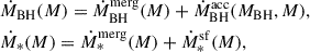
  is the stellar mass growth rate by star formation. The baryonic gas sources the latter two terms, and, consequently, the evolution of the BH and stellar masses is coupled through the SN and AGN feedback processes that can heat or eject parts of the baryonic gas (Bower et al. 2006, 2017; Dubois et al. 2015; Habouzit et al. 2017). We utilised a phenomenological fit to the star formation rate shown by the yellow curve in Fig. 1 (see Appendix B for details). This accounts for the SN and AGN feedback and is based on the results of Harikane et al. (2022), which has been tested successfully with new JWST data (Harikane et al. 2023b). Following Dayal et al. (2019), we consistently accounted for the effect of the SN feedback (Dayal et al. 2014), which strongly suppresses the BH accretion in halos lighter than M ≈ 5 × 10¹¹ M⊙ so that only the fraction frem shown by the red curve in Fig. 1 is available for accretion. Moreover, we limited the average accretion to the Eddington rate3. According to Piana et al. (2020) and Bower et al. (2017), these are approximately the conditions necessary to explain the UV AGN luminosity function, but rather than an ad hoc cut on the SMBH mass where accretion is started, it is a consequence of the interpretation of the star formation fit.
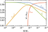 |
Fig. 1. Baryon fractions as functions of DM halo mass M. fej is the cold gas fraction that is ejected from the halo by SNe, fcold is the fraction of the remaining gas that is cold, frem is the fraction of gas available for accretion, and f* is the fraction of cold gas that is used for star formation. |
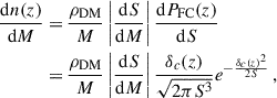
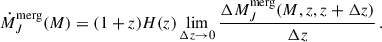
We used the EPS formalism to model the growth by mergers. The growth rate by mergers is given by the Δz ≡ z′−z → 0 limit of (see Appendix A)
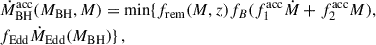
![Mathematical equation: $$ \begin{aligned} \begin{aligned}&\Delta M_J^\mathrm{merg}(M,z,z^{\prime }) = \int _0^M \mathrm{d} M^{\prime } \bigg |\frac{\mathrm{d} S}{\mathrm{d} M^{\prime }}\bigg | \frac{M}{M^{\prime }} M_J(M^{\prime },z^{\prime })\\&\quad \times \frac{\delta _c(z^{\prime })-\delta _c(z)}{\sqrt{2\pi [S(M^{\prime })-S(M)]^3}}e^{-\frac{[\delta _c(z^{\prime })-\delta _c(z)]^2}{2[S(M^{\prime })-S(M)]}} - M_J(M,z^{\prime }), \end{aligned} \end{aligned} $$](/articles/aa/full_html/2025/11/aa55389-25/aa55389-25-eq5.gif) (2)
(2)
where J = BH, *, S(M) denotes the variance of the DM perturbations and δc(z) is the threshold DM density contrast for halo formation. We assumed the cold DM model and computed S(M) and δc(z) following Dodelson (2003) and Eisenstein & Hu (1998), with the cosmological parameters inferred from the CMB observations (Planck Collaboration VI 2020).
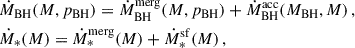
We also considered the possibility that not all mergers are efficient at forming a tight BH binary that merges quickly. We parametrised this with an efficiency parameter, 0 ≤ pBH ≤ 1, which multiplies the BH growth rate by mergers if it is positive4. High merger efficiency, pBH ≃ 1, might be a good approximation if the SMBH is surrounded by a nuclear star cluster, which is very effective at lowering the orbital timescale (Mukherjee et al. 2025). However, it might be too optimistic for a more general case and should be considered an effective upper value. Studies of the efficiency of mergers induced by dark matter or three-body effects indicate a reduced BH merger efficiency pBH ∼ 𝒪(0.1) (Zhou et al. 2025), although with a big uncertainty5.
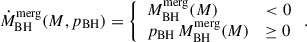
We initiated the evolutionary process by planting a seed of mass mseed at a given redshift (zseed) in every halo that is heavier than a given minimal mass, Mseed, and we evolve the BH masses and stellar masses by solving the coupled Equations (1) numerically. We note that we only evolved the expected BH mass, MBH = ∫dP(mBH) mBH, and do not include the inevitable scatter in the present computations. We therefore estimated the occupation fractions with Dirac delta functions:
![Mathematical equation: $$ \begin{aligned} \frac{\mathrm{d} P(m_{\rm BH}|M_*,z)}{\mathrm{d} m_{\rm BH}} = \frac{M_{\rm BH}(M_*,z)}{m_{\rm BH}} \delta \left[m_{\rm BH} - m_{\rm BH}(M_*,z)\right], \end{aligned} $$](/articles/aa/full_html/2025/11/aa55389-25/aa55389-25-eq6.gif) (3)
(3)
where
![Mathematical equation: $$ \begin{aligned} m_{\rm BH}(M_*,z) = \max \left[m_{\rm seed},M_{\rm BH}(M_*,z)\right] \end{aligned} $$](/articles/aa/full_html/2025/11/aa55389-25/aa55389-25-eq7.gif) (4)
(4)
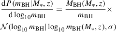
corresponds to the proper BH mass. To explore how a spread in the results could affect the comparison with the data, we can replace the Dirac delta function in Eq. (3) with a log-normal distribution, 𝒩(log10mBH|log10mBH(M*, z),σ)/mBH, where  denotes the Gaussian distribution with mean
  and the variances σ2, as discussed below.
3. Implications of the data
We used the stellar mass-BH mass data from previous works (Übler et al. 2023; Larson et al. 2023; Harikane et al. 2023a; Bogdan et al. 2024; Ding et al. 2023; Maiolino et al. 2024; Yue et al. 2024; Kocevski et al. 2023; Stone et al. 2024) for the JWST AGNs, the high-redshift quasar masses compiled by Izumi et al. (2021), and the data concerning local AGNs and IGs (where SMBH masses are measured dynamically) compiled by Reines & Volonteri (2015). Examples of our model predictions for the stellar mass-BH mass correlation for pBH = 1 are shown alongside the data in Fig. 2. The benchmark cases shown correspond to examples with light seeds (mseed = 100 M⊙ and Mseed = 3 × 10⁴ M⊙) and heavy seeds (mseed = 105 M⊙ with Mseed = 3 × 10⁷ M⊙). The bend in the model predictions at M* ∼ 1010 M⊙ arises because SN feedback expels all of the gas remaining after star formation below a critical halo mass, preventing efficient BH accretion. Therefore, growth via mergers is the dominant growth channel for BHs in such light galaxies. Light-seed scenarios have enough light BHs to fuel the growth of the AGNs observed by the JWST, but the heavy-seed model predictions undershoot the JWST observations for M* ≲ 109 M⊙. The high-z quasar data with M* ≳ 1010 M⊙ compiled by Izumi et al. (2021) are, instead, fitted well by either light or heavy seeds. In the right panel of Fig. 2, we see that both the low-z IGs and the low-z AGN data are fitted well thanks to the steep fall of the model predictions at M* ∼ 1011 − 1010 M⊙ arising from the SN feedback.
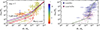 |
Fig. 2. Comparisons of model predictions for stellar mass-BH mass relation with high-z observations on the left and low-z observations on the right. The solid lines show the evolution of light seeds (mseed = 100 M⊙ with Mseed = 3 × 10⁴ M⊙), and dashed lines show the evolution of heavy seeds (mseed = 105 M⊙ with Mseed = 3 × 10⁷ M⊙), both for pBH = 1. The right panel shows the predictions of the same two models at z ≈ 0 as full and dashed lines, respectively, compared to the local observations. |
We compare the qualities of our model predictions to the stellar mass-BH mass observations using the likelihood function
 (5)
(5)
where the product is over the data points and the Gaussian probability densities  account for the uncertainties in the measurements of the BH masses and the galaxy stellar masses. Fixing all the parameters associated with star formation by observations, the free parameters are those associated with the formation of the first generation of massive BHs and the efficiency factor of the BH growth by mergers:
 (6)
(6)
We find that varying zseed ∈ (15 − 20) does not significantly affect the likelihood. The following results were calculated for fixed zseed = 20.
We performed scans over mseed and Mseed for fixed values of pBH = 1 and pBH = 0.1, as mentioned above. In Fig. 3, we show the posterior distributions for each of the different data sets, ignoring a possible spread in the mass relation. The upper left plot displays results for fits to the high-z quasar data compiled by Izumi et al. (2021). We see that, whilst these data favour a strong correlation between mseed and Mseed, they do not favour any particular range of seed masses. This reflects the observation that the predictions of both the light- and heavy-seed models pass through the high-z SMBH data compiled by Izumi et al. (2021). On the other hand, as seen in the upper right plot, the JWST data show a preference for light seeds with masses of mseed ≲ 103 M⊙ if pBH = 1 and heavier seeds with masses of 104 M⊙ ≲ mseed ≲ 105 M⊙ if pBH = 0.1. The low-z observations, shown in the lower panels, also show strong correlations between the seed halo mass and the seed BH mass, with the contours scaling roughly as  , but they do not constrain the seed BH mass significantly by themselves.
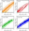 |
Fig. 3. Fits to stellar mass-BH mass data as functions of seed BH mass mseed and minimal halo mass, Mseed, where the seeds are inserted at zseed = 20 with pBH = 1 in solid and pBH = 0.1 in dashed. The contours indicate the 68%, 95%, and 99% credible regions. Upper left: High-z quasar data compiled by Izumi et al. (2021). Upper right: High-z observations with JWST (Übler et al. 2023; Larson et al. 2023; Harikane et al. 2023a; Bogdan et al. 2024; Ding et al. 2023; Maiolino et al. 2024; Yue et al. 2024). Lower left: Low-z AGNs as compiled by Reines & Volonteri (2015). Lower right: Low-z IGs from Reines & Volonteri (2015). |
In Fig. 4, we compare the fit combining the low-z data and the high-z quasar data with the fit to the JWST high-z data. We note that the trend of the fit to the high-z quasar data is slightly steeper than for the low-z data,  , which is why the fit combining the low-z data and the high-z quasar data shown in grey in Fig. 4 has a preferred seed mass range. The JWST fit shows a preference for lighter seeds than the combined fit. This preference is stronger for pBH = 1 than for pBH = 0.1, but even for pBH = 1 the fits overlap significantly within the 2σ confidence level. In Fig. 5, we show the evolution of the (mseed, Mseed) relation for the best fits to JWST data and the rest of the SMBH data for pBH = 0.1: parameter values are given in Table 1. We see how the JWST-only fit, shown as solid lines, traverses the data and has the correct z dependence. On the other hand, the fit to the rest of the data, shown as dashed lines, reproduces the local data better.
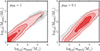 |
Fig. 4. Fits to stellar mass-BH mass data; the red posteriors show the fit to the JWST data, and the grey posteriors show the fit combining the low-z data and the high-z quasar data. |
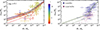 |
Fig. 5. Comparisons of model predictions for stellar mass-BH mass relation with high-z observations on the left and with low-z observations on the right. The solid lines show the best fit for pBH = 0.1 to the JWST data, and the dashed lines show the best fit to the rest of the SMBH data. The best-fit parameter values are given in Table 1. |
Likelihood comparison.
The JWST and other datasets exhibit significant scatter, with objects both above and below the model predictions, while the fits presented in Figs. 3 and 4. assume zero spread in the model predictions. To explore whether our results are sensitive to spread in our model predictions, we repeated the analysis including a log-normal spread with σ = 0.5 in the predicted SMBH mass. The fits are shown in the supplemental material. Our overall conclusions do not change, but the preference of the fit moves to slightly smaller seed masses and the quality of the fit improves. We collected best fits from the different scans in Table 1, which also shows the best fits obtained for a power-law fit as in Ellis et al. (2024b). Impressively, our model provides significantly better fits than the power-law fit with the same number of degrees of freedom. Moreover, we see that a spread in the model predictions clearly improves the quality of the fit, and the data prefer a lower merger efficiency of pBH = 0.1 over pBH = 1, independently of the spread. However, we also see that, in particular for pBH = 0.1, the seed BHs need to be relatively heavy compared to the minimal halo masses where they are planted; on the other hand, the JWST data become more compatible with the rest of the SMBH data.
Lambrides et al. (2024) (see also Pacucci & Narayan 2024) raised the possibility that the masses of at least some of the JWST SMBHs (Maiolino et al. 2024) may have been overestimated. It has been argued that the non-detection of measurable X-rays or UV emission lines suggests that these SMBHs may be lower mass objects accreting at super-Eddington rates. As seen in Fig. 2 of Lambrides et al. (2024), this argument would reduce the estimated masses of some SMBHs observed with the JWST (Maiolino et al. 2024) by perhaps an order of magnitude. This would shift the preference of the JWST data towards seeds planted in heavier halos.
4. Conclusions
In this paper, we presented a new semi-analytical model of the co-evolution of SMBHs and their host galaxies. This model is based on estimates of the growth rate of BH masses and the galaxy stellar masses derived from the EPS formalism and on phenomenological modelling of star formation, SN, and AGN feedback processes and BH accretion. In particular, we included the suppression of BH accretion in halos lighter than ≈5 × 10¹¹ M⊙ due to SN feedback and a parameter that describes how efficient the halo mergers are at forming a tight BH binary. Our approach involves solving numerically coupled differential equations for the evolution of the SMBH masses and the stellar masses and is much faster than approaches based on merger trees or numerical simulations. This allowed us to perform a systematic study of different SMBH seeding scenarios, including scans of the model parameter space.
Our model predicts BH mass-stellar mass relations that are compatible with the observations. We find that the heavy seed scenarios where BHs of mass ∼105 M⊙ are planted in halos heavier than ∼107 M⊙ undershoot the JWST observations because the BHs in halos lighter than ≈5 × 10¹¹ M⊙ grow predominantly by mergers, but there are not enough BHs to merge with. Scenarios with lighter seeds planted into lighter halos are preferred by the JWST as they allow for more efficient growth of the BHs by mergers.
We performed a likelihood analysis scanning over the seed BH masses and the masses of the smallest halos into which they are planted. As seen in Table I, our analysis suggests that the JWST data prefer lighter seeds, mseed ≲ 103 M⊙ if the merging efficiency is high, pBH = 1, but the preference moves to higher masses, 104 M⊙ ≲ mseed ≲ 105 M⊙, for a lower merger efficiency of pBH = 0.1. The other data from local observations and observations of high-z quasars instead prefer the higher seed-mass range, 104 M⊙ ≲ mseed ≲ 105 M⊙, for both pBH = 1 and pBH = 0.1. The fits have two non-trivial successes. First, the fits are better for pBH = 0.1, which aligns with a fit to the PTA GW background (Ellis et al. 2024a). Secondly, our model provides a much better fit than those obtained with a simple power-law parametrisation (Ellis et al. 2024b), as also seen in Table I.
Our model does not resolve the spread in the BH masses, but we explored the effects of the spread by parametrising it. We find that including the spread significantly improves the fit to the observations, as also seen in Table I. This is expected given that the data exhibit significant scatter. The inclusion of the spread in the model predictions also prefers slightly lower seed masses but does not change the overall conclusions (see Fig. C.3).
Building on the success of our model framework to study the scatter in the range of SMBH masses for any given value of the stellar mass is clearly a priority. Another interesting extension of this work would be to calculate the magnitude of the stochastic GW background due to BH binaries to higher frequencies than those explored by the PTAs that could be explored by LISA (Amaro-Seoane et al. 2017) and deciHz experiments (Badurina et al. 2020; El-Neaj et al. 2020; Kawamura et al. 2021). However, these explorations lie beyond the scope of this paper.
The full evolution from z = 20 to z = 0, with Δz = 0.1, takes ≈2 min on an eight-core M2 Apple processor, resolving the halos down to 1 M⊙.
The merger efficiency pBH describes the probability of a halo merger leading to a merger of the central BHs.
We note that the BH accretion can include periods of super-Eddington accretion during galaxy mergers and periods of less efficient accretion. In our model, the growth through both mergers and accretions is described as an average over a long time.
This approach has been used in, for example, Ricarte & Natarajan (2018). We emphasise that it is a simplification and could be improved by including a time delay with some spread between the halo merger and the merger of the central BHs, among other things. We leave such improvements for future work.
This is also consistent, within large uncertainties, with the merger efficiency needed to explain the PTA GW background with inspiralling SMBH binaries (Ellis et al. 2024a).
Acknowledgments
This work was supported by the Estonian Research Council grants PRG803, PSG869, RVTT3 and RVTT7 and the Center of Excellence program TK202. The work of J.E. and M.F. was supported by the United Kingdom STFC Grants ST/T000759/1 and ST/X000753/1. The work of V.V. was partially supported by the European Union’s Horizon Europe research and innovation program under the Marie Skłodowska-Curie grant agreement No. 101065736.
References
- Afzal, A., Agazie, G., Anumarlapudi, A., et al. 2023, ApJ, 951, L11 [Erratum: ApJ 971, L27 (2024)] [NASA ADS] [CrossRef] [Google Scholar]
- Agazie, G., Anumarlapudi, A., Archibald, A. M., et al. 2023a, ApJ, 951, L8 [NASA ADS] [CrossRef] [Google Scholar]
- Agazie, G., Alam, Md F., Anumarlapudi, A., et al. 2023b, ApJ, 951, L9 [CrossRef] [Google Scholar]
- Amaro-Seoane, P., Audley, H., Babak, S., et al. 2017, arXiv e-prints [arXiv:1702.00786] [Google Scholar]
- Badurina, L., Bentine, E., Blas, D., et al. 2020, JCAP, 05, 011 [CrossRef] [Google Scholar]
- Bhowmick, A. K., Blecha, L., Ni, Y., et al. 2022, MNRAS, 516, 138 [NASA ADS] [CrossRef] [Google Scholar]
- Bhowmick, A. K., Blecha, L., Torrey, P., et al. 2024a, MNRAS, 533, 1907 [Google Scholar]
- Bhowmick, A. K., Blecha, L., Torrey, P., et al. 2024b, MNRAS, 531, 4311 [NASA ADS] [CrossRef] [Google Scholar]
- Bi, Y.-C., Wu, Y.-M., Chen, Z.-C., & Huang, Q.-G. 2023, Sci. China Phys. Mech. Astron., 66, 120402 [NASA ADS] [CrossRef] [Google Scholar]
- Bogdan, A., Goulding, A. D., Natarajan, P., et al. 2024, Nat. Astron., 8, 126 [Google Scholar]
- Bower, R. G., Benson, A. J., Malbon, R., et al. 2006, MNRAS, 370, 645 [Google Scholar]
- Bower, R. G., Schaye, J., Frenk, C. S., et al. 2017, MNRAS, 465, 32 [NASA ADS] [CrossRef] [Google Scholar]
- Correa, C. A., Wyithe, J. S. B., Schaye, J., & Duffy, A. R. 2015, MNRAS, 450, 1514 [NASA ADS] [CrossRef] [Google Scholar]
- Croton, D. J., Springel, V., White, S. D. M., et al. 2006, MNRAS, 365, 11 [Erratum: MNRAS 367, 864 (2006)] [Google Scholar]
- Dayal, P., Ferrara, A., Dunlop, J., & Pacucci, F. 2014, MNRAS, 445, 2545 [CrossRef] [Google Scholar]
- Dayal, P., Rossi, E. M., Shiralilou, B., et al. 2019, MNRAS, 486, 2336 [Google Scholar]
- Ding, X., Onoue, M., Silverman, J. D., et al. 2023, Nature, 621, 51 [NASA ADS] [CrossRef] [Google Scholar]
- Dodelson, S. 2003, Modern Cosmology (Amsterdam: Academic Press) [Google Scholar]
- Dubois, Y., Volonteri, M., Silk, J., et al. 2015, MNRAS, 452, 1502 [Google Scholar]
- Eisenstein, D. J., & Hu, W. 1998, ApJ, 496, 605 [Google Scholar]
- Ellis, J., Fairbairn, M., Hütsi, G., et al. 2024a, Phys. Rev. D, 109, L021302 [NASA ADS] [CrossRef] [Google Scholar]
- Ellis, J., Fairbairn, M., Hütsi, G., et al. 2024b, A&A, 691, A270 [NASA ADS] [CrossRef] [EDP Sciences] [Google Scholar]
- Ellis, J., Fairbairn, M., Franciolini, G., et al. 2024c, Phys. Rev. D, 109, 023522 [NASA ADS] [CrossRef] [Google Scholar]
- El-Neaj, Y. A., Alpigiani, C., Amairi-Pyka, S., et al. 2020, EPJ Quant. Technol., 7, 6 [CrossRef] [Google Scholar]
- EPTA Collaboration and InPTA Collaboration (Antoniadis, J., et al.) 2023, A&A, 678, A50 [CrossRef] [EDP Sciences] [Google Scholar]
- EPTA Collaboration and InPTA Collaboration (Antoniadis, J., et al.) 2024, A&A, 685, A94 [NASA ADS] [CrossRef] [EDP Sciences] [Google Scholar]
- Figueroa, D. G., Pieroni, M., Ricciardone, A., & Simakachorn, P. 2024, Phys. Rev. Lett., 132, 171002 [NASA ADS] [CrossRef] [Google Scholar]
- Habouzit, M., Volonteri, M., & Dubois, Y. 2017, MNRAS, 468, 3935 [NASA ADS] [CrossRef] [Google Scholar]
- Harikane, Y., Ono, Y., Ouchi, M., et al. 2022, ApJS, 259, 20 [NASA ADS] [CrossRef] [Google Scholar]
- Harikane, Y., Zhang, Y., Nakajima, K., et al. 2023a, ApJ, 959, 39 [NASA ADS] [CrossRef] [Google Scholar]
- Harikane, Y., Ouchi, M., Oguri, M., et al. 2023b, ApJS, 265, 5 [NASA ADS] [CrossRef] [Google Scholar]
- Izumi, T., Matsuoka, Y., Fujimoto, S., et al. 2021, ApJ, 914, 36 [CrossRef] [Google Scholar]
- Kawamura, S., Ando, M., Ando, M., et al. 2021, PTEP, 2021, 05A105 [Google Scholar]
- Klessen, R. S., & Glover, S. C. O. 2023, ARA&A, 61, 65 [NASA ADS] [CrossRef] [Google Scholar]
- Kocevski, D. D., Onoue, M., Inayoshi, K., et al. 2023, ApJ, 954, L4 [NASA ADS] [CrossRef] [Google Scholar]
- Kulkarni, M., Visbal, E., & Bryan, G. L. 2021, ApJ, 917, 40 [NASA ADS] [CrossRef] [Google Scholar]
- Lacey, C. G., & Cole, S. 1993, MNRAS, 262, 627 [NASA ADS] [CrossRef] [Google Scholar]
- Lambrides, E., Garofali, K., Larson, R., et al. 2024, arXiv e-prints [arXiv:2409.13047] [Google Scholar]
- Larson, R. L., Finkelstein, S. L., Kocevski, D. D., et al. 2023, ApJ, 953, L29 [NASA ADS] [CrossRef] [Google Scholar]
- Latif, M. A., & Ferrara, A. 2016, PASA, 33, e051 [NASA ADS] [CrossRef] [Google Scholar]
- Li, J., Silverman, J. D., Shen, Y., et al. 2025, ApJ, 981, 19 [Google Scholar]
- Lupi, A., Trinca, A., Volonteri, M., Dotti, M., & Mazzucchelli, C. 2024, A&A, 689, A128 [NASA ADS] [CrossRef] [EDP Sciences] [Google Scholar]
- Madau, P. 2025, ApJ, submitted [arXiv:2501.09854] [Google Scholar]
- Maiolino, R., Scholtz, J., Curtis-Lake, E., et al. 2024, A&A, 691, A145 [NASA ADS] [CrossRef] [EDP Sciences] [Google Scholar]
- Marulli, F., Bonoli, S., Branchini, E., Moscardini, L., & Springel, V. 2008, MNRAS, 385, 1846 [CrossRef] [Google Scholar]
- Mukherjee, D., Zhou, Y., Chen, N., Di Carlo, U. N., & Di Matteo, T. 2025, ApJ, 981, 203 [Google Scholar]
- Naoz, S., & Barkana, R. 2007, MNRAS, 377, 667 [Google Scholar]
- Natarajan, P., Pacucci, F., Ricarte, A., et al. 2024, ApJ, 960, L1 [NASA ADS] [CrossRef] [Google Scholar]
- Pacucci, F., & Narayan, R. 2024, ApJ, 976, 96 [NASA ADS] [CrossRef] [Google Scholar]
- Pacucci, F., Nguyen, B., Carniani, S., Maiolino, R., & Fan, X. 2023, ApJ, 957, L3 [CrossRef] [Google Scholar]
- Piana, O., Dayal, P., Volonteri, M., & Choudhury, T. R. 2020, MNRAS, 500, 2146 [Google Scholar]
- Piana, O., Pu, H.-Y., & Wu, K. 2024, MNRAS, 530, 1732 [Google Scholar]
- Planck Collaboration VI. 2020, A&A, 641, A6 [Erratum: A&A 652, C4 (2021)] [NASA ADS] [CrossRef] [EDP Sciences] [Google Scholar]
- Raidal, J., Urrutia, J., Vaskonen, V., & Veermäe, H. 2024, A&A, 691, A212 [NASA ADS] [CrossRef] [EDP Sciences] [Google Scholar]
- Reardon, D. J., Zic, A., Shannon, R. M., et al. 2023, ApJ, 951, L6 [NASA ADS] [CrossRef] [Google Scholar]
- Reines, A. E., & Volonteri, M. 2015, ApJ, 813, 82 [NASA ADS] [CrossRef] [Google Scholar]
- Ricarte, A., & Natarajan, P. 2018, MNRAS, 474, 1995 [Google Scholar]
- Schauer, A. T. P., Glover, S. C. O., Klessen, R. S., & Clark, P. 2021, MNRAS, 507, 1775 [NASA ADS] [CrossRef] [Google Scholar]
- Schaye, J., Crain, R. A., Bower, R. G., et al. 2015, MNRAS, 446, 521 [Google Scholar]
- Sijacki, D., Vogelsberger, M., Genel, S., et al. 2015, MNRAS, 452, 575 [NASA ADS] [CrossRef] [Google Scholar]
- Stone, M. A., Lyu, J., Rieke, G. H., Alberts, S., & Hainline, K. N. 2024, ApJ, 964, 90 [NASA ADS] [CrossRef] [Google Scholar]
- Toubiana, A., Sberna, L., Volonteri, M., et al. 2025, A&A, 700, A135 [NASA ADS] [CrossRef] [EDP Sciences] [Google Scholar]
- Tremmel, M., Karcher, M., Governato, F., et al. 2017, MNRAS, 470, 1121 [NASA ADS] [CrossRef] [Google Scholar]
- Trinca, A., Schneider, R., Valiante, R., et al. 2022, MNRAS, 511, 616 [NASA ADS] [CrossRef] [Google Scholar]
- Übler, H., Maiolino, R., Curtis-Lake, E., et al. 2023, A&A, 677, A145 [NASA ADS] [CrossRef] [EDP Sciences] [Google Scholar]
- Volonteri, M., Lodato, G., & Natarajan, P. 2008, MNRAS, 383, 1079 [Google Scholar]
- Volonteri, M., Habouzit, M., & Colpi, M. 2021, Nat. Rev. Phys., 3, 732 [NASA ADS] [CrossRef] [Google Scholar]
- Xu, H., Chen, S., Guo, Y., et al. 2023, Res. Astron. Astrophys., 23, 075024 [CrossRef] [Google Scholar]
- Yue, M., Eilers, A.-C., Simcoe, R. A., et al. 2024, ApJ, 966, 176 [NASA ADS] [CrossRef] [Google Scholar]
- Zhou, Y., Mukherjee, D., Chen, N., et al. 2025, ApJ, 980, 79 [Google Scholar]
Appendix A: Going beyond halo merger trees
Although the EPS formalism is a convenient way to derive halo merger trees and thereby BH histories, it has its drawbacks, mainly that halos with masses below ∼108 M⊙ are too abundant and computationally expensive to include (although this can be improved by an adaptive resolution (Toubiana et al. 2025)). In this paper, we aim to overcome these drawbacks by applying the EPS formalism directly to the evolution of SMBHs without invoking the halo merger tree step. The key insight behind this approach is that a SMBH inside a halo on average, has had the same history as the average mass element of the halo. This implies that the statistics from the random paths for the mass elements of a halo at some (M, z) are the same as for the SMBH inside that halo, which is the key assumption used when their evolution is calculated using halo merger trees.
In the cold dark matter model, the variance of matter perturbations S(M) is a monotonically decreasing function of the halo mass M: S(M)→0 as M → ∞. Thus, we can replace M by S ≡ S(M) and the matter overdensity field δ around each spatial point evolves along a path in the (S(M),δ) plane that originates from (0, 0). The first crossing of the path across a threshold value δc(z) determines the halo mass M around that point at redshift z. We compute the threshold δc(z) as in Dodelson (2003) and the variance S(M) following Eisenstein & Hu (1998), with the cosmological parameters fixed by the CMB observations (Planck Collaboration VI 2020).
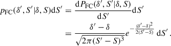
Assuming that the fluctuations are Gaussian, the probability a path to get to the point (S, δ) is 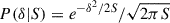 and the probability that the first crossing is at variance larger than S is given by
![Mathematical equation: $$ \begin{aligned} \begin{aligned} P_{\rm FC}(S,z)&= 1 - \int _{-\infty }^{\delta _c(z)}\mathrm{d} \delta \, \left[P(\delta |S) - P(2\delta _c(z)-\delta |S) \right] \\&= 1 - \mathrm{erf}\left[\frac{\delta _c(z)}{\sqrt{2 S}}\right] \,. \end{aligned} \end{aligned} $$](/articles/aa/full_html/2025/11/aa55389-25/aa55389-25-eq16.gif) (A.1)
(A.1)
This is the cumulative mass fraction in halos lighter than M and the EPS halo mass function (HMF) is simply
 (A.2)
(A.2)
where ρDM is the present average DM energy density.
If the path is not initiated in (0, 0) but instead at (S, δ), the probability to get to the point (S′,δ′), S′> S becomes P(δ′|δ, S, S′) = P(δ′−δ|S′−S). The probability for a path starting at (S, δ) to cross the threshold δ′=δc(z′) > δ = δc(z) at variance larger than S′ is, in the same way as in (A.1), given by
![Mathematical equation: $$ \begin{aligned} \begin{aligned} P_{\rm FC}(\delta ^{\prime },S^{\prime }|\delta ,S) = 1 - \mathrm{erf}\left[\frac{\delta ^{\prime }-\delta }{\sqrt{2(S^{\prime }-S)}}\right] \,, \end{aligned} \end{aligned} $$](/articles/aa/full_html/2025/11/aa55389-25/aa55389-25-eq18.gif) (A.3)
(A.3)
and the probability for the path to cross the threshold δ′ in the range (S′,S′+dS′) is
 (A.4)
(A.4)
From this one can compute what fraction of the mass M of a halo at z on average comes from a halo of mass M′ in the past, z′> z. If instead, we want to compute how the mass of the halo M′ at z′ is going to be distributed in heavier halos M > M′ in some later time z < z′, we need to invert the conditional probability (A.3). This gives the probability that a path that starts at (δ′,S′) crosses the threshold δ in the range (S, S + dS) (see Eq. (2.16) in Lacey & Cole (1993)):
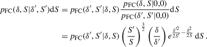 (A.5)
(A.5)
A change of variables then gives the probability that the halo whose mass at z′ is M′ ends up being a part of a halo in the mass range (M, M + dM) at z < z′:
 (A.6)
(A.6)
This allows us to compute the evolution of the HMF forward in time from z′> z to z as
 (A.7)
(A.7)
It is easy to check that this formula holds by inserting the HMF (A.2) in the right-hand side and performing the integral. We estimate the growth rate of the DM halos by computing the expected growth of the halo through mergers with smaller halos:
![Mathematical equation: $$ \begin{aligned} \dot{M} = (1+z) H(z) \lim _{\Delta z \rightarrow 0} \frac{1}{\Delta z} \left[\frac{\int _{M}^{2M} \! \mathrm{d} \tilde{M}\, \tilde{M} \frac{\mathrm{d} P(\tilde{M},z|M,z+\Delta z)}{\mathrm{d} \tilde{M}}}{\int _{M}^{2M} \! \mathrm{d} \tilde{M}\, \frac{\mathrm{d} P(\tilde{M},z|M,z+\Delta z)}{\mathrm{d} \tilde{M}}} - M \right] \,. \end{aligned} $$](/articles/aa/full_html/2025/11/aa55389-25/aa55389-25-eq23.gif) (A.8)
(A.8)
We show in Fig. A.1 DM halo growth rates calculated using Eq. (A.8) (solid lines) and, for comparison, estimates derived in Correa et al. (2015), which is based on finding the average mass of the main progenitor. The agreement is generally good over the range of halo masses M relevant for our study.
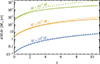 |
Fig. A.1. Calculations of the growth rates of DM halos. The solid curves are obtained using Eq. (A.8) and used in our analysis. The dashed curves show for comparison the estimates derived in Correa et al. (2015), which are based on finding the average mass of the main progenitor. |
Appendix B: SMBHs and baryonic physics
The average BH mass and the stellar mass evolve according to the coupled equations
 (B.1)
(B.1)
where  , J = (BH, * ,gas), denotes the growth rate by mergers,
  denotes BH accretion rate, and
  is the star formation rate. The baryonic matter (stars and gas) and the SMBH have the same progenitors as the DM halo that hosts them. So, considering only mergers, their expected masses, MJ, evolve from z′ to z in a halo of mass M as
![Mathematical equation: $$ \begin{aligned} \begin{aligned}&M_J(M,z^{\prime }) + \Delta M_J^\mathrm{merg}(M,z,z^{\prime })=\\&\left[\frac{\mathrm{d} n(z)}{\mathrm{d} M}\right]^{-1}\!\! \int _0^M \mathrm{d} M^{\prime }\,\frac{\mathrm{d} n(z^{\prime })}{\mathrm{d} M^{\prime }} \frac{\mathrm{d} P(M,z|M^{\prime },z^{\prime })}{\mathrm{d} M} M_J(M^{\prime },z^{\prime }) =\\&\int _0^M \mathrm{d} M^{\prime } \bigg |\frac{\mathrm{d} S}{\mathrm{d} M^{\prime }}\bigg |\times \\&\frac{M}{M^{\prime }} M_J(M^{\prime },z^{\prime }) \frac{\delta _c(z^{\prime })-\delta _c(z)}{\sqrt{2\pi [S(M^{\prime })-S(M)]^3}}e^{-\frac{[\delta _c(z^{\prime })-\delta _c(z)]^2}{2[S(M^{\prime })-S(M)]}} \,. \end{aligned} \end{aligned} $$](/articles/aa/full_html/2025/11/aa55389-25/aa55389-25-eq28.gif) (B.2)
(B.2)
The growth rate by mergers is given by the limit
 (B.3)
(B.3)
For the growth rate of BHs by mergers,  , we considered the possibility that not all mergers are efficient at forming a tight binary and the consequent BH is left orbiting at very high separations and it is no longer efficient at accreting or merging. In that case, we considered
 (B.4)
(B.4)
The part 1 − pBH of the accreted SMBH mass can be thought of as an SMBH that is left wandering in the galaxy or becomes ejected and does not play any significant role in future mergers.
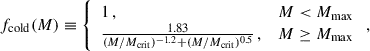
Our aim in the following is to utilise phenomenological fits as much as possible while combining the different components in a physically consistent manner. We start from the star formation rate found in Harikane et al. (2022), based on fitting the UV luminosity function
![Mathematical equation: $$ \begin{aligned} \begin{aligned} \dot{M}_*^\mathrm{sf}(M,z)&= \frac{6.4\times 10^{-2}[0.53\tanh {\left(0.54(2.9-z)\right)}+1.53]}{(M/M_{\rm crit})^{-1.2}+(M/M_{\rm crit})^{0.5}} \dot{M} \\&= f_*(M,z) f_{\rm cold}(M) f_B \dot{M} \end{aligned} \end{aligned} $$](/articles/aa/full_html/2025/11/aa55389-25/aa55389-25-eq32.gif) (B.5)
(B.5)
with Mcrit = 1011.5 M⊙. Stars are formed from the cold baryonic gas. In the second line of (B.5) we have factorised the fit into the fraction of cold gas,
 (B.6)
(B.6)
and the effective star formation efficiency, which determines the fraction of cold gas that is converted to stars,
![Mathematical equation: $$ \begin{aligned} \begin{aligned}&f_*(M,z) \equiv \left[ 0.33 + 0.12\tanh {\left(0.54(2.9-z)\right)} \right] \times \\&{\left\{ \begin{array}{ll} \frac{1.83}{(M/M_{\rm crit})^{-1.2}+(M/M_{\rm crit})^{0.5}} \,,&M < M_{\rm max} \\ 1 \,,&M\ge M_{\rm max} \end{array}\right.} \,. \end{aligned} \end{aligned} $$](/articles/aa/full_html/2025/11/aa55389-25/aa55389-25-eq34.gif) (B.7)
(B.7)
The mass Mmax = 5.3 × 10¹¹ M⊙ corresponds to the maximum of  . Finally, we define the fraction of the cold gas that is ejected from the halo or pushed away from the central region so it is not available for the SMBH to accrete, by supernovae (SNe) as
 (B.8)
(B.8)
This means that the cold gas used for star formation is sufficient for the feedback from the resulting SNe to expel the remaining gas. Star formation reaches its maximum at M = Mmax, and the SNe are no longer able to eject all the gas at M > Mmax. Therefore, for M > Mmax there is still gas available to fuel AGN activity, which has the effect of heating the gas in the galaxy, leading to a downturn in the star formation, as illustrated in Fig. 1. The evolution of stellar masses is fixed by the star formation rate (B.5), the EPS estimate for the halo growth (A.8) and the growth of stellar masses by mergers (B.3). We show the resulting evolution of the halo mass-stellar mass relation in Fig. B.1.
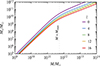 |
Fig. B.1. The evolution of the halo mass-stellar mass relation given by the star formation rate (B.5), the EPS estimate for the halo growth (A.8) and the growth of stellar masses by mergers (B.3). |
The amount of gas left in the halo after the star formation period is available for accretion by the SMBH. Following Dayal et al. (2019), we estimate the BH accretion rate as
 (B.9)
(B.9)
where f1acc = 5.5 × 10⁻⁴ and f2acc = 5 × 10⁻⁵/Myr is the fraction of the available gas that can be accreted by the SMBH,
 (B.10)
is the total fraction of gas left after star formation and ejection of gas by SNe, fEdd is the fraction of the Eddington rate at which the SMBHs can maximally accrete and the Eddington accretion rate is given by
 (B.11)
where mp is the proton mass and σT is the Thomson cross section. The physical interpretation is that in low-mass halos, the SN feedback prevents efficient accretion, and in heavy halos, the accretion is limited by the Eddington rate and the amount of available gas.
We initiate the evolution by planting a seed of mass mseed at some redshift zseed in all halos that are heavier than some minimal mass Mseed. Note that we evolve only the expected BH mass, MBH = ∫dP(mBH) mBH, and do not include the inevitable scatter in the present computations. We therefore estimate the occupation fractions with Dirac delta functions
![Mathematical equation: $$ \begin{aligned} \frac{\mathrm{d} P(m_{\rm BH}|M_*,z)}{\mathrm{d} m_{\rm BH}} = \frac{M_{\rm BH}(M_*,z)}{m_{\rm BH}} \delta \left[m_{\rm BH} - m_{\rm BH}(M_*,z)\right] \,, \end{aligned} $$](/articles/aa/full_html/2025/11/aa55389-25/aa55389-25-eq40.gif) (B.12)
(B.12)
where
![Mathematical equation: $$ \begin{aligned} m_{\rm BH}(M_*,z) = \max \left[m_{\rm seed},M_{\rm BH}(M_*,z)\right] \end{aligned} $$](/articles/aa/full_html/2025/11/aa55389-25/aa55389-25-eq41.gif) (B.13)
(B.13)
corresponds to the proper BH mass. This is the BH mass that enters the accretion rate in Eq. (B.11) and that we compare with observations in the main text. For clarity, Table B.1 compiles the parameters related to the accretion and growth of the BHs.
Parameters of the model
Appendix C: Effects of spread and astrophysical implications for the seeds
As mentioned above, our model calculations are for means in the distribution of SMBH masses, and do not include the inevitable spread. Including this within the growth formalism we have described would cause the simple additive process to become a nonlinear convolution. In order to explore how a spread could change the results, we include an ad-hoc spread in the distribution of BH masses only in the final comparison with the data, but the evolution is computed only using the mean of the distribution. We use the lognormal distribution
 (C.1)
(C.1)
for this purpose, and assume σ = 0.5. Results from modifying the distribution in this way are shown in Fig. C.1 for pBH = 1, in Fig. C.2 for pBH = 0.1 and in Fig. C.3 for the JWST and the combination of all other data, and included in Table 1, and are commented in the main text.
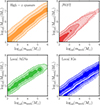 |
Fig. C.1. Fits to the stellar mass-BH mass data as functions of the seed BH mass mseed and minimal halo mass Mseed where the seeds are inserted at zseed = 20, for pBH = 1 without spread in the predicted relation in solid and with a log-normal spread (σ = 0.5) in dashed. |
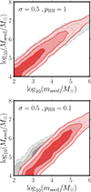 |
Fig. C.3. As in Fig. 4, allowing for a lognormal spread in the model predictions with σ = 0.5 for pBH = 1 in the left panel and for pBH = 0.1 in the right panel. |
We also compare the results from our fit to astrophysically motivated models for the seeds. In particular, we focus on Mseed, the minimal halo mass to form SMBHs. The best fit to all the data was achieved at pBH = 0.1 and, as seen in Fig. C.4, the halo mass where the seeds are embedded aligns nicely with the simulations from Schauer et al. (2021), Kulkarni et al. (2021), and is compatible at the 2σ CL with the analytical estimation of atomic cooling halos at z = 20. It is also compatible at the 3σ CL with a very light halo mass, which has been found by Naoz & Barkana (2007) to be able to host Pop-III stars in simulations. This wide range of results from the simulations is what has motivated our prior range for Mseed. The SMBH mass is the most uncertain part of the seeding process. The best fit seems to be achieved for ”heavy" halos, close to the atomic cooling halos range, that require heavy seeds with masses ∼105 M⊙, which could be associated with a direct collapse scenario, see Latif & Ferrara (2016) for a review. The typical light-seed scenario, in which heavy Pop-III stars collapse to BHs of 𝒪(102 M⊙) (Klessen & Glover 2023) for a review, seems to be viable only if the Pop-III stars can form in very light minihalos of 𝒪(104 M⊙). For heavier values of the minimal halo mass to form the Pop-III stars, either the Pop-III stars are very heavy 𝒪(104 M⊙) or there are 𝒪(102) per halo that can merge efficiently, otherwise the direct collapse scenario seems to be a more viable option.
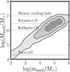 |
Fig. C.4. Comparison of our best fit to all the data, with pBH = 0.1, with respect to different values from simulations on Mseed (Schauer et al. 2021; Kulkarni et al. 2021; Naoz & Barkana 2007), as well as the atomic cooling halo estimation at z = 20. The implications of the fit for the viability of posteriors in astrophysical terms are discussed in Sec. C. |
All Tables
All Figures
|
Fig. 1. Baryon fractions as functions of DM halo mass M. fej is the cold gas fraction that is ejected from the halo by SNe, fcold is the fraction of the remaining gas that is cold, frem is the fraction of gas available for accretion, and f* is the fraction of cold gas that is used for star formation. |
| In the text | |
|
Fig. 2. Comparisons of model predictions for stellar mass-BH mass relation with high-z observations on the left and low-z observations on the right. The solid lines show the evolution of light seeds (mseed = 100 M⊙ with Mseed = 3 × 10⁴ M⊙), and dashed lines show the evolution of heavy seeds (mseed = 105 M⊙ with Mseed = 3 × 10⁷ M⊙), both for pBH = 1. The right panel shows the predictions of the same two models at z ≈ 0 as full and dashed lines, respectively, compared to the local observations. |
| In the text | |
|
Fig. 3. Fits to stellar mass-BH mass data as functions of seed BH mass mseed and minimal halo mass, Mseed, where the seeds are inserted at zseed = 20 with pBH = 1 in solid and pBH = 0.1 in dashed. The contours indicate the 68%, 95%, and 99% credible regions. Upper left: High-z quasar data compiled by Izumi et al. (2021). Upper right: High-z observations with JWST (Übler et al. 2023; Larson et al. 2023; Harikane et al. 2023a; Bogdan et al. 2024; Ding et al. 2023; Maiolino et al. 2024; Yue et al. 2024). Lower left: Low-z AGNs as compiled by Reines & Volonteri (2015). Lower right: Low-z IGs from Reines & Volonteri (2015). |
| In the text | |
|
Fig. 4. Fits to stellar mass-BH mass data; the red posteriors show the fit to the JWST data, and the grey posteriors show the fit combining the low-z data and the high-z quasar data. |
| In the text | |
|
Fig. 5. Comparisons of model predictions for stellar mass-BH mass relation with high-z observations on the left and with low-z observations on the right. The solid lines show the best fit for pBH = 0.1 to the JWST data, and the dashed lines show the best fit to the rest of the SMBH data. The best-fit parameter values are given in Table 1. |
| In the text | |
|
Fig. A.1. Calculations of the growth rates of DM halos. The solid curves are obtained using Eq. (A.8) and used in our analysis. The dashed curves show for comparison the estimates derived in Correa et al. (2015), which are based on finding the average mass of the main progenitor. |
| In the text | |
|
Fig. B.1. The evolution of the halo mass-stellar mass relation given by the star formation rate (B.5), the EPS estimate for the halo growth (A.8) and the growth of stellar masses by mergers (B.3). |
| In the text | |
|
Fig. C.1. Fits to the stellar mass-BH mass data as functions of the seed BH mass mseed and minimal halo mass Mseed where the seeds are inserted at zseed = 20, for pBH = 1 without spread in the predicted relation in solid and with a log-normal spread (σ = 0.5) in dashed. |
| In the text | |
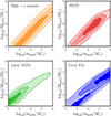 |
Fig. C.2. As in Fig. C.1 for pBH = 0.1. |
| In the text | |
|
Fig. C.3. As in Fig. 4, allowing for a lognormal spread in the model predictions with σ = 0.5 for pBH = 1 in the left panel and for pBH = 0.1 in the right panel. |
| In the text | |
|
Fig. C.4. Comparison of our best fit to all the data, with pBH = 0.1, with respect to different values from simulations on Mseed (Schauer et al. 2021; Kulkarni et al. 2021; Naoz & Barkana 2007), as well as the atomic cooling halo estimation at z = 20. The implications of the fit for the viability of posteriors in astrophysical terms are discussed in Sec. C. |
| In the text | |
Current usage metrics show cumulative count of Article Views (full-text article views including HTML views, PDF and ePub downloads, according to the available data) and Abstracts Views on Vision4Press platform.
Data correspond to usage on the plateform after 2015. The current usage metrics is available 48-96 hours after online publication and is updated daily on week days.
Initial download of the metrics may take a while.