| Issue |
A&A
Volume 703, November 2025
|
|
|---|---|---|
| Article Number | A92 | |
| Number of page(s) | 18 | |
| Section | Extragalactic astronomy | |
| DOI | https://doi.org/10.1051/0004-6361/202555450 | |
| Published online | 07 November 2025 | |
The soft X-ray transient EP241021A: A cosmic explosion with a complex off-axis jet and cocoon from a massive progenitor
1
INAF – Istituto di Astrofisica e Planetologia Spaziali, Via Fosso del Cavaliere 100, I-00133 Rome, Italy
2
Department of Physics, University of Bath, Claverton Down, Bath BA2 7AY, UK
3
Instituto de Astrofísica de Andalucía (IAA-CSIC), Glorieta de la Astronomía s/n, 18008 Granada, Spain
4
Key Laboratory of Particle Astrophysics, Institute of High Energy Physics, Chinese Academy of Sciences, Beijing 100049, China
5
South-Western Institute for Astronomy Research, Yunnan University, Kunming, Yunnan 650500, China
6
Faculty of Science, University of Helsinki, Gustaf Hällströmin katu 2a, P.O. Box 64 FI-00014 Helsinki, Finland
7
Institute of Physics and Technology, Ural Federal University, Mira str. 19, 620002 Ekaterinburg, Russia
8
Department of Astronomy, School of Physics and Technology, Wuhan University, Wuhan 430072, China
9
Guangxi Key Laboratory for Relativistic Astrophysics, School of Physical Science and Technology, Guangxi University, Nanning 530004, China
10
National Astronomical Observatories, Chinese Academy of Sciences, Beijing 100101, China
11
School of Astronomy and Space Science, University of Chinese Academy of Sciences, Chinese Academy of Sciences, Beijing 100049, China
12
INAF – Osservatorio di Astrofisica e Scienza dello Spazio, Via Piero Gobetti 93/3, I-40129 Bologna, Italy
13
INAF – Istituto di Radioastronomia, Via P. Gobetti 101, 40129 Bologna, Italy
14
ARIES – Aryabhatta Research Institute of Observational Sciences, Nainital 263001, India
15
INAF – Osservatorio Astronomico di Roma, Via Frascati 33, Monte Porzio Catone 00078, Italy
⋆ Corresponding author: This email address is being protected from spambots. You need JavaScript enabled to view it.
Received:
8
May
2025
Accepted:
7
September
2025
Abstract
Context. X-ray flashes (XRFs) are fast X-ray transients discovered by the BeppoSAX satellite. Diverse evidence indicates that XRFs are connected to gamma ray bursts (GRBs) and likely represent their softer analogs. With its soft X-ray bandpass and exquisite sensitivity, the Einstein Probe (EP) offers a novel opportunity to disclose the nature of such puzzling events.
Aims. Several models have been proposed to explain the observed properties of XRFs, mostly in the context of the collapsar scenario, where such soft events could have different geometrical or physical conditions of the progenitor with respect to GRBs. These include off-axis GRBs and baryon-loaded explosions, which either produce a low-Lorentz-factor jet or a spherical, mildly (or non-) relativistic ejecta, known as cocoons. In this paper, we present multiwavelength observations of the afterglow of EP241021a, a soft X-ray transient detected by EP. We attempt to connect the complex, multicomponent afterglow emission with leading XRF models.
Methods. We first characterize the prompt emission of EP2410121a by EP-WXT and Fermi-GBM. Then, we present the results of our multiwavelength campaign from radio (uGMRT, ATCA, e-MERLIN, and ALMA), optical (LBT, GTC, and CAHA) and X-rays (EP-FXT). We perform an analysis of light curves and broad-band spectra using both empirical and physical models of GRBs and spherical expansions (both nonrelativistic and mildly relativistic cocoons).
Results. The EP241021a afterglow is characterized by multiple components, which represent the imprints of the interaction of a jet with the complex environment of the preexisting progenitor that is likely shaping its structure. In particular, the optical and X-ray afterglows are well described by a structured jet with wide and low-Lorentz-factor (γ ∼ 40) wings, which produce the decreasing light curve before 6 days. A re-brightening at 7 days in the optical and X-ray data is due to the jet core, which is off-axis and coming into view. The radio emission can be modeled with a mildly relativistic cocoon (γ ∼ 2). Finally, in the radio spectrum at 70 days, we find an additional component peaking at ∼50 GHz, which is well described by a second cocoon with γ ∼ 1
Key words: radiation mechanisms: non-thermal / relativistic processes / gamma-ray burst: general
© The Authors 2025
 Open Access article, published by EDP Sciences, under the terms of the Creative Commons Attribution License (https://creativecommons.org/licenses/by/4.0), which permits unrestricted use, distribution, and reproduction in any medium, provided the original work is properly cited.
This article is published in open access under the Subscribe to Open model. This email address is being protected from spambots. You need JavaScript enabled to view it. to support open access publication.
1. Introduction
The key properties of long gamma ray bursts (GRBs) are successfully explained by the so-called “collapsar” scenario. After the core-collapse explosion of a stripped-envelope massive star – likely a rapidly rotating Wolf-Rayet (WR, Yoon & Langer 2005) – matter flows toward a newly formed black hole or rapidly spinning, highly magnetized neutron star (Woosley 1993; MacFadyen & Woosley 1999), and a relativistic jet breaks free from the stellar progenitor along the polar axis (MacFadyen & Woosley 1999; Aloy et al. 2000). Internal shocks produce the gamma ray (prompt emission) and, when the ejecta reach the circumstellar medium, they emit the afterglow (detected in X-ray, optical, and radio bands). The observer can be within the jet cone angle (on-axis) or outside it (off-axis). When on-axis, prompt emission in the gamma rays is observed; instead, when viewed off-axis, either no prompt emission or some less energetic emission from the tails of the jet may be observed.
However, the collapsar scenario also predicts the presence of additional components – jetted or spherical (Gottlieb et al. 2020; Salafia et al. 2020; Ramirez-Ruiz et al. 2002; MacFadyen et al. 2001) – which can manifest depending on various conditions. Before the relativistic jet exits the progenitor star, part of the energy output is deposited into a “cocoon” surrounding it. As the jet head breaks out of the progenitor star, the cocoon plasma can escape swiftly from the stellar cavity and accelerate. Instead, as the cocoon itself breaks out of the stellar envelope, prompt emission in the soft keV energies may be seen prior to the typical gamma-ray emission of GRBs. These precursors have already been observed in a small number of GRBs (recently in Liu et al. 2025; but see also Piro et al. 2005; Lazzati 2005).
There is also the possibility that the jet is polluted by baryons (the so-called baryon-loaded jet). While long-duration GRB afterglows are powered by explosions that have minimal initial ejecta mass, typically 10−6 M⊙, in the baryon-loaded case the jet has a mass of M ∼ 10−5 − 10−3 M⊙. In this case, the jet does not reach the high Lorentz factors (10 < γ0 < 100) necessary to produce a prompt emission in the gamma rays, and the prompt emission is expected in the soft X-rays. The expected initial energies are similar to GRBs, 1051 − 1053 erg (MacFadyen et al. 2001; Huang et al. 2004). If baryon loading is high, the jet can also be choked entirely (choked-jet scenario), but a small amount of spherical and relativistic ejecta is still launched (Chakraborti & Ray 2011). The observational signature in this scenario is either a relativistic supernova (SN, as SN 2012ap with a mass > 10−2.5 M⊙, Chakraborti et al. 2015; Margutti et al. 2014; Soderberg et al. 2010), or a classical nonrelativistic SN (with a mass of 0.1 M⊙).
Observations of GRBs in the context of the collapsar model typically reveal only the presence of a relativistic jet. In fact, there is only limited evidence suggesting that baryon-loaded explosions can produce low-luminosity GRBs, such as GRB 060218 (Campana et al. 2006; Soderberg et al. 2006), GRB 100316D (Starling et al. 2011; Margutti et al. 2013), GRB 980425 (Pian et al. 1999), and GRB 031203 (Watson et al. 2004). This is likely attributable to the dominance of relativistic jet emission over other potential components, but it begs the question whether such other components, expected in the collapsar scenario, can shape other classes of cosmic explosions. X-ray flashes (XRFs) are a very promising candidate. They are fast X-ray transients discovered by the BeppoSAX satellite (Heise 2003), classified as GRBs with absent (or very low) gamma-ray emission. Including the somewhat harder X-ray-rich (XRR) GRBs, they make up about two-thirds of GRB events observed by BeppoSAX or HETE2 (Piro & Hurley 2012, for a review). This interesting class of events can potentially bridge the gap between highly collimated and relativistic jets and baryon-loaded explosions and cocoons.
The XRFs show an isotropic distribution on the sky and a duration of the prompt emission between 10–1000 seconds. The observed prompt X-ray properties are similar to those of GRBs, except for the softer peak energy of the spectrum (Barraud et al. 2003; D’Alessio et al. 2006). For example, several follow the Amati–Yonetoku relation (Willingale & Mészáros 2017). Several pieces of evidence (including prompt phase observations by BeppoSAX and HETE-2; see Sakamoto et al. 2008) indicate that these transients are connected to GRBs and most likely represent their softer analogs. They lie at extragalactic distances, with host galaxies not unlike those of long GRBs (Chen et al. 2021; D’Alessio et al. 2006), and they often have similar X-ray to radio afterglow emission (Bi et al. 2018; Chandra & Frail 2012; Sakamoto et al. 2008; Gendre et al. 2007; D’Alessio et al. 2006). Many XRFs are also associated with SNe (Bi et al. 2018), which further supports that they share the same origin as GRBs.
Even if they are likely associated with the collapsar scenario, the XRF emission origin is still unclear. Several models have been proposed to explain the observed properties in the context of the collapsar scenario depicted above. The main ones are:
(1) Off-axis GRBs (Zhang et al. 2003; Yamazaki et al. 2002; Granot et al. 2002, 2005; Urata et al. 2015). In this case, the observer’s viewing angle (the angle between the line of sight and the jet axis) is outside the jet’s cone. The narrow, collimated relativistic jet (emitting gamma rays) is not seen, but the jet tail emission at lower Lorentz factors can still be detected in X-rays. From their afterglows, however, there is no compelling evidence of XRFs coming from off-axis jets (D’Alessio et al. 2006).
(2) Baryon-loaded or choked jets, also called sub-energetic or inefficient fireballs (Huang et al. 2002; Rhoads 2003; Dermer et al. 2000; Zhang & Mészáros 2002), which also lead to the cocoon emission mentioned before. In this case, the ejecta are less energetic than a GRB jet and therefore emit the prompt emission in the X-rays.
(3) GRBs at such high redshifts that the observed peak is moved into the X-ray band (Heise 2003). This, however, can be excluded as the only source of XRFs, as this should also result in fainter afterglows, which are not observed (D’Alessio et al. 2006). Moreover, the detected redshifts have a mean value of z ∼ 1 (Bi et al. 2018).
In recent years, finding such bursts with low luminosity and softer spectral peak energies has been difficult because of instruments designed to trigger on GRBs with high keV energies. However, some Swift GRBs, such as GRB 201015A, can be classified as XRFs (Patel et al. 2023). With the advent of the X-ray mission Einstein Probe (EP), launched in January 2024, the population of XRFs is growing. In particular, the Wide-field X-ray Telescope (WXT) on board EP is characterized by an extremely large field of view (3600 deg2), good sensitivity, and a soft energy band (0.5–4 keV, Yuan et al. 2022, 2025).
In this work, we present an extensive dataset of the afterglow of EP241021a, a fast X-ray transient discovered by EP. Since there were no detections by Fermi-GBM and Konus-Wind, this transient is consistent with XRF properties (see Section 2.1). In Section 2.2 we introduce the X-ray, optical, and radio datasets. Their spectral and temporal behavior is studied phenomenologically in Section 3.1. In Section 3.2 we physically interpret the complete light curve and spectra, placing the features we obtained from the physical modeling in the context of collapsars in Section 4. Finally, the conclusions are given in Section 5.
2. Observations
2.1. Prompt emission
EP241021a was detected by the EP-WXT on October 21, 2024 (Hu et al. 2024). The transient started at 2024-10-21T05:07:56 (UTC, T0 hereafter) and had a duration of about 100 seconds. The average 0.5–4 keV spectrum is well fit by an absorbed power law with a photon index of 1.8 and a column density fixed at the Galactic value of 5 × 1020 cm−2, with an average unabsorbed 0.5–4 keV flux of  (Shu et al. 2025). This translates into a fluence in the 2–30 keV band of ∼6 × 10⁻⁸ erg cm−2.
There is no high-energy (gamma-ray) counterpart of this event. In particular, Fermi-GBM operated as expected at that time, and the position of the transient was not Earth-occulted. We extracted the Fermi-GBM light curve of the nb detector, (the nearest to the source position) using the Fermi Gamma-ray Data Tools (Goldstein et al. 2023). Modeling the background as a first-order power law, we find a rate of two counts per second. This leads to a 3σ upper limit (Gehrels 1986) on the fluence in the 30–400 keV band assuming a duration of 100 s of: 1 × 10⁻⁶ erg cm−2 for a long GRB spectrum (Band function with α = −1, β = −2.5, and peak energy Ep = 300 keV); 5 × 10⁻⁷ erg cm−2 for an XRR spectrum (Band function with α = −1, β = −2.5, and peak energy Ep = 70 keV); and 2 × 10⁻⁷ erg cm−2 for an XRF spectrum (Band function with α = −1, β = −2.5, and peak energy Ep = 30 keV). In addition, Konus-Wind also observed the whole sky at the time of the transient but did not detect the source (Svinkin et al. 2024).
Following D’Alessio et al. (2006) and depending on the ratio of the fluences in the bands F(2−30 keV)/F(30−400 keV), we classify this transient as either a GRB (F(2−30 keV)/F(30−400 keV) < 0.3), an X-ray-rich GRB (1 < F(2−30 keV)/F(30−400 keV) < 0.3), or an XRF (F(2−30 keV)/F(30−400 keV) > 1). Assuming an XRF spectrum, the upper limit on the 30–400 keV and the 2–30 keV fluences places this transient in the XRR and XRF population, with F(2−30 keV)/F(30−400 keV) ≥ 0.3.
The spectroscopic redshift is observed to be 0.75 (Pérez-Fournon et al. 2024; Pugliese et al. 2024; Zheng et al. 2024). This gives a 0.5–10 keV luminosity of 1.3 × 1048 erg s−1, which is consistent with low-luminosity GRBs, and very similar to EP240414a luminosity in the same band (Sun et al. 2025).
Due to the uncertainty on the photon index  found in Shu et al. (2025), it is difficult to constrain the peak energy Epeak of the spectrum. We find that for Epeak ≥ 30 keV (Eiso ∼ 1052 erg), the transient is marginally consistent with the Amati relation (Willingale & Mészáros 2017).
2.2. Afterglow
2.2.1. Einstein Probe FXT
The Follow-up X-ray Telescope (FXT, Chen et al. 2020a) on board EP operates in the 0.3–10 keV band and consists of two co-aligned modules (FXT-A and FXT-B). EP241021a was observed for fifteen total epochs by EP-FXT, starting from 2024-10-22 to 2025-01-08. Data were reduced using the recommended procedures from the FXT Data Analysis Software v1.10: particle event identification, pulse invariant conversion, grade calculation and selection (grade ≲ 12), bad- and hot-pixel flagging and selection of good time intervals using the housekeeping file to produce cleaned event files. The cleaned event files were then filtered for background flares, after which images and spectra were extracted for further analysis.
For source detection, we performed the recommended checks for EP-FXT data1, employing an S/N (signal-to-noise ratio) threshold of three. The source was detected at nine epochs out of the fifteen. We estimated the source count rates from a 1 arcmin circle (corresponding to 95% of the FXT point spread function – PSF), centered on the e-MERLIN position (see Section 2.2.5), and the background rates from an annulus with an inner radius of 1.2 and outer radius of 2.5 arcmin (thus, away from the source PSF and at least three times larger in area). Upper limits for the six non-detections were derived by taking the single-sided 3σ Poissonian confidence limit following the procedure from Gehrels (1986).
We calculated an unabsorbed counts-to-flux conversion factor by assuming the best-fit spectral parameters of the observation at 8 days post-event (06800000186), where we had the most significant late-time detection of the X-ray counterpart. The spectra for this epoch were fit with an absorbed power law, with a single absorption component fixed to the Galactic neutral column in the direction of EP241021a (5 × 1020 cm−2) and from which we derived a best-fit photon index Γ of 1.81 ± 0.30. This yields a counts-to-flux conversion factor of 3.1 × 10⁻¹¹. We also individually fit all the FXT observations with a detection and found a photon index consistent within errors with 1.81 ± 0.30, indicating negligible spectral evolution. When we had a detection in both modules, we derived the final count rate as the average of those from the FXT-A and FXT-B telescopes. The results of the FXT data reduction are compiled in Table A.1. We jointly fit the spectra with the highest number of counts up to 6.0 days, with an absorbed power law (the single absorption component fixed to the Galactic neutral column), deriving a best-fit photon index of Γ = 1.92 ± 0.22. Finally, we also jointly fit all the FXT spectra from 1.5 to 8.6 days with the same model, deriving a best-fit photon index of Γ = 1.80 ± 0.20, in agreement with the analysis of Shu et al. (2025).
2.2.2. LBT
We observed the optical counterpart of EP241021a with the Large Binocular Cameras (Giallongo et al. 2008) mounted on the Large Binocular Telescope (LBT; Mt. Graham, AZ, USA) and obtained simultaneous r′ and z′ imaging on 2024-10-28, at midtime UT 06:25:00, 7.05 days after the burst (Program IT-2024B-023, PI Elisabetta Maiorano). Observations were performed under an average seeing of 0 85 for a total of 600 s in each filter. Imaging data were reduced using the dedicated data reduction pipeline (Fontana et al. 2014). All data were analyzed by performing aperture photometry using DAOPHOT and APPHOT under PyRAF/IRAF, and calibrated against the SDSS DR12 catalog magnitudes of brighter nearby stars (Alam et al. 2015). The optical afterglow was well detected in all bands. We measure an AB magnitude of r′ = 21.78 ± 0.02 and z′ = 21.25 ± 0.03, not corrected for the foreground Galactic extinction Aλ (Aλ = 0.11 in the r′ band and Aλ = 0.065 in the z′ band).
2.2.3. GTC
Near-IR observations with the 10.4-meter Gran Telescopio Canarias (GTC) in La Palma (Canary Islands, Spain) in the JHK-bands were conducted with the IR multi-object spectrograph EMIR (Espectrografo Multiobjeto Infra-Rojo) on two epochs (November 13, 2024, and February 3, 2025) with total on-source times of 350 s (J), 462 s (H), and 588 s (Ks) each time, under program GTCMULTIPLE7B-24B. Data were reduced using the standard EMIR pipeline and calibrated using the 2MASS catalog. Observations are reported in Table A.2, not corrected for Aλ, with Aλ = 0.037, 0.02 and 0.02 in the J, H, Ks bands, respectively.
2.2.4. CAHA
Optical observations with the 2.2-meter Calar Alto Telescope (CAHA) in southern Spain were conducted with the Calar Alto Faint Object Spectrograph (CAFOS) in the g′r′i′z′- Sloan bands on December 7 and 8, 2024, under program 24B-2.2-012, with on-source exposures of 840 s g′, 630 s r′, and 360 s i′ (December 7) and 900 s r′ and 900 s i′ (December 8). Data were reduced using the standard IRAF routine and calibrated using the Sloan Digital Survey Photometric Catalog. Observations are reported in Table A.2, not corrected for Aλ, with Aλ = 0.17, 0.11 and 0.09 in the g′, r′, and i′ bands, respectively.
2.2.5. e-MERLIN
We began observations of EP241021a on October 24, 2024, under our approved Target-of-Opportunity e-MERLIN (enhanced Multi Element Remotely Linked Interferometer Network) project CY18212 (PI: Gianfagna) and monitored the source for four epochs (see Table A.3) at 5.5 GHz. Each run lasted ∼12 hours, alternating between target and phase calibrator. Data were calibrated with the e-Merlin pipeline (Moldon 2021), and then imaged in CASA (Common Astronomy Software Applications, The CASA Team 2022), reaching a typical angular resolution of ∼150 × 50 milli-arcsec, and an RMS of ∼50 μJy/beam. Observation results are reported in Table A.3.
2.2.6. ATCA
We monitored the source for a total of six epochs with the Australia Telescope Compact Array (ATCA) starting on October 29, 2024, through our approved program C3638 (PI: Gianfagna) and the shared program CX585 (PIs: Carotenuto, Gianfagna, Troja, Yao). Observations were carried out with the 16 cm (2.1 GHz), 4 cm (5.5 GHz and 9 GHz), and 15 mm (16.7 GHz and 21.2 GHz) receivers, in phase referencing mode. Data were processed in CASA (The CASA Team 2022), with standard recipes. The combination of different array configurations during the approximately three-month campaign, and the equatorial declination of the target, made imaging challenging for some epochs. In such cases, resulting in an extremely elongated beam, we measured the source flux density through a direct fitting of the interferometer visibilities with the UVMODELFIT task in CASA. Otherwise, when imaging was feasible, we extracted the peak flux density in a region centered on the source position. Results are reported in Table A.3.
2.2.7. GMRT
We obtained director discretionary time (DDT) through the project ddtC407 (PI: Gianfagna) with GMRT (Giant Metrewave Radio Telescope). We performed two epochs with a total of 8 hours, divided among Band 3 (250–500 MHz), Band 4 (550–580 MHz), and Band 5 (1050–1450 MHz). Observations were conducted on December 30–31, 2024, and March 23, 2025. Data were processed with the SPAM pipeline2. For the first epoch, we reached an RMS of 155 μJy/beam in Band-3, and 24 μJy/beam in Band-5, while Band-4 failed to produce a usable image due to data corruption by RFI (radio frequency interference). We observed only in Band-5 for the second epoch, reaching an RMS of 38 μJy/beam. No detection was achieved at either epoch (see Table A.3 for the resulting upper limits).
2.2.8. ALMA
Another DDT was granted by the Atacama Large Millimeter/submillimeter Array (ALMA) with code 2024.A.00019.T (PI: Gianfagna). Observations were carried out in the period of December 28–30, 2024, for a total of 11 min on source in Band 1, with central frequency 40 GHz, and 2.5 h on source in Band 6, with central frequency 233 GHz. The data have been calibrated using the pipeline (version 2024.1.0.8) and images have been obtained using the task tclean in CASA (version 6.6.1.7; The CASA Team 2022). The multifrequency synthesis of the data over the full bandwidth (∼7.5 GHz) resulted in a rms of 15 μJy/beam (4.46 × 3.525 arcsec) in Band 1, and of 10 μJy/beam (0.7 × 0.6 arcsec) in Band 6. We obtained in both bands detections of point-like sources with a S/N larger than 10, and the corresponding flux densities (with their error) are reported in Table A.3. As a quality check, we also obtained images of the four different spectral windows, and the source does not show any significant in-band variation in flux.
3. Analysis
The broadband light curve of the afterglow of EP241021a is presented in Fig. 1. While the optical and X-rays are observed to decrease with time, the radio band shows a rising phase and a peak around 30 days.
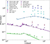 |
Fig. 1. EP241021a broadband light curve. FXT observations are represented with green data points; optical observations are represented in shades of purple and pink; and radio data are represented in shades of blue. Inverted triangles indicate upper limits. The optical data represented with circles are taken from the literature (Busmann et al. 2025, 2024; Aryan et al. 2025; Fu et al. 2024a,b; Li et al. 2024; J-Jin et al. 2024; Pan et al. 2024; Ror et al. 2024; Kumar et al. 2024; Bochenek & Perley 2024a,b,c; Freeburn et al. 2024a,b; Quirola-Vasquez et al. 2024; Moskvitin & Spiridonova 2024a,b,c; Schneider & Adami 2024). The solid black lines and shaded-colored regions represent the best fit and the 500 best likelihood fits of the data using power law models. |
The X-ray afterglow luminosity is observed to span the order of 1044 − 1045 erg s−1. At early times before the bump, the emission was placed at the lower end of cosmological GRBs, between the majority of the GRB population and low-luminosity GRBs, such as GRB060218, GRB100316D, and GRB980425 (see Fig. 2, left panel). The radio luminosity further supports this association (see Fig. 2, right panel). Instead, the late X-ray luminosity is consistent with the standard GRB population. This could suggest that the EP241021a X-ray emission after the peak is likely due to a relativistic jet, while the early X-ray and the full radio light curve could be due to a less energetic component. As an example, nonrelativistic flows (such as SNe type Ic) can be clearly rejected as they have luminosities on the order of 1028 erg s−1 Hz−1 at 9 GHz.
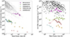 |
Fig. 2. Left panel: X-ray luminosities in the 0.3–10 keV band of Swift-detected GRBs (Evans et al. 2007, 2009). Right panel: Radio afterglow luminosities at 9 GHz of the GRB catalog presented in Chandra & Frail (2012). EP241021a is represented in magenta stars, while low-luminosity GRBs, such as GRB 060218 (Campana et al. 2006; Soderberg et al. 2006), GRB 100316D (Starling et al. 2011; Margutti et al. 2013), GRB 980425 (Pian et al. 1999), and GRB 031203 (Watson et al. 2004) are represented with light blue, yellow, light red, and green squares, respectively, in both panels. |
In the following sections, we analyze the EP241021a light curve and broadband spectrum using a phenomenological approach and a physical interpretation. The fits are performed using the Python package Dynesty (Higson et al. 2019; Speagle 2020; Koposov et al. 2024), and the corner plot is made using corner (Foreman-Mackey 2016). The results are always presented as median, 16th, and 84th percentiles.
3.1. Phenomenological analysis
3.1.1. Light curve
We assumed a time and spectral dependence for the flux of the type F ∝ tανβ and fit the light curve in X-rays, the r band, and at 5–5.5 GHz with smoothly broken power laws. In the case of the radio band, we find slopes αr, 1 = 1.2 ± 0.1 and αr, 2 = −1.2 ± 0.1 and break time  d. In the case of the optical, we find that the early (t < 6 d) light curve has a slope of αo, 0 = −0.70 ± 0.03, then there is a fast rising slope of αo, 1 = 4.6 ± 1.5, a bump with
  d and a decreasing slope of αo, 2 = −1.26 ± 0.05 (all in agreement with Busmann et al. 2025). In the X-rays, the early slope is
  , then αx, 1 = 3.1 ± 1.2, a bump with
  d and a decreasing slope of αo, 2 = −2.3 ± 0.5. The slopes α1 and peak times of the optical and X-ray light curves agree within 1σ, while the slopes α2 seem to suggest a milder decrease in the optical flux. The X-ray slope is consistent with a post-jet break phase.
Focusing on optical and X-rays, we first considered the early afterglow emission, up to about 7 days. The different slopes suggest that, assuming a synchrotron emission, a break frequency is between the two bands. According to the afterglow theory, in an ISM (interstellar medium) environment (Sari et al. 1998), the flux at high frequencies is expected to decrease faster with time than at lower frequencies, contrary to what is observed. However, in the case of a wind environment (Chevalier & Li 2000), the optical light curve can be steeper than the X-ray, with a difference of 1/4. EP241021a does show a steeper slope for the optical band, suggesting a wind environment, but the difference from the X-rays is ∼0.4. Such a large difference can be explained by continuous energy injection due to refreshing material. The latter can produce milder decays. We thus use this model to explain the early afterglow emission in Section 3.2.1. The bump and the ensuing decay observed in optical and X-rays will be discussed in more detail in Section 3.2.2.
3.1.2. Spectrum
We repeated the same analysis for the broadband spectrum. We used a three-broken power law model, fixing the slopes of each power law to the slopes expected in the synchrotron modeling. In particular, from low to high energies, the slopes are 2, 1/3, −(p − 1)/2, and p/2, in the assumption of slow cooling. The fitted parameters are then p and three break frequencies: the synchrotron self-absorption νsa, the injection νm, and the cooling νc frequencies. The spectra at ∼8 d and ∼25 d are represented in Fig. 3. At 8 days, we could only get an upper limit on the synchrotron self-absorption frequency, νsa < 5.5 GHz. The same occurred for νc, for which we obtained a lower limit of ∼2.5 × 10¹⁷ Hz. We find  ,
,  , and a normalization
  mJy. The value of p is in agreement with the one estimated from the X-ray spectrum (Section 2.2.1): assuming that X-rays are below νc, this leads to a spectral slope β = Γ − 1 = (p − 1)/2 = 0.8 ± 0.2, and p = 2.6 ± 0.4. At 25 days, the spectral peak appeared to be at ∼5 GHz. Assuming that this is still νm, this would correspond to a time dependence of ∼t−4, hardly explainable with synchrotron theory. We note that all the radio spectra, except the one at 8 days, exhibit the same bell shape. This is also reported in Shu et al. (2025). Hence, radio emission after ∼25 days is likely produced by a component separated from the one responsible for the optical and X-ray afterglow. For this reason, we fit the 25 d broadband spectrum with the sum of two different components, one for the radio and one for the optical. We discuss the radio spectrum in detail later, while here we focus on the optical. We always assumed a three-broken power-law model, imposing that νm evolves from 8 days onward following a time dependence of νm ∝ t−3/2, which is valid both for wind and ISM environments. The fit is represented with the dashed line in the second panel of Fig. 3. We find
  ,
,  , and a normalization
  while νsa and νc are unconstrained. This result clearly shows the presence of a separate component in the radio band (see Fig. 3, bottom panel and the following text), a result independent of the value of νsa.
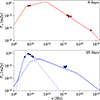 |
Fig. 3. EP241021a broadband spectrum at ∼8 d (top panel) and ∼25 d (bottom panel). In the top panel, the solid lines represent a fit of two broken power law models. In the bottom panel, the solid line represents the sum of the radio and optical components, represented with dotted and dashed lines, respectively. |
We now turn to the radio spectrum, which we fit with one smoothly broken power law. The fitted parameters are the two slopes β1 and β2 before and after the break frequency νb, and the peak flux Fb. We show the epochs at 25 d in Fig. 3, bottom panel, and 70 d in Fig. 4. The results are reported in Table 1. Interestingly, at 70 days, the spectrum is double-peaked, with a second peak emerging in the ALMA bandpass, and we use the sum of two smoothly broken power laws to fit the data. In the table, we report the results of the fit for both components, represented in Fig. 4.
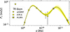 |
Fig. 4. EP241021a radio spectrum at 70 days. The 5 sigma upper limits from uGMRT are represented as triangles; ATCA observations are represented with dots; and ALMA observations are represented with stars. The spectra are fit with a broken power-law model, the colored regions represent the 500 highest-likelihood fits, while the black line represents the best fit. |
Phenomenological fit of the radio spectra.
The power law spectral shape mentioned above confirms a synchrotron origin also for the EP241021a radio afterglow. A rising slope between ∼2–2.5 is expected when synchrotron self-absorption is dominant; thus, the break frequency νb corresponds to νsa. In particular, a slope of β1 ≈ 2.5 is expected when the electron injection frequency is below the self-absorption frequency (νm < νsa). This order is further supported by the absence of a ν1/3 regime above the break frequency. In fact, in our observations, higher frequencies are following a power law with a slope between −1.4 and −0.8, and are all in agreement within 2σ. In the case of slow cooling synchrotron emission, such slopes would correspond to −(p − 1)/2, leading to a mean value of p of 3.1 ± 0.5.
The break frequency νsa has a value of 5 GHz at 25 d. If we assume a GRB synchrotron spectrum, in the case of a wind environment, νsa is given by
 (1)
(1)
The main contributions to νsa are by ϵe and A* (Chevalier & Li 2000). Assuming E0 = 1052 erg and ϵB = 0.1, having νsa = 5 GHz would mean an extremely high density of A* = 6 × 103 cm−1 for ϵe = 0.1, in contrast with the highest end of the GRB distribution of 10 (Aksulu et al. 2022). In the case of a GRB in an ISM, νsa is given by
 (2)
(2)
Assuming the same values as above for E0 and ϵB, to get νsa = 5 GHz, for ϵe = 0.1 an extremely high density n0 ≃ 105 cm−3 is needed also in this case, with respect to typical ISM densities on the order of unity, or lower. Such high densities both in the wind and ISM environments are not only in disagreement with GRB studies, but also influence other afterglow traits, as the jet break time tjb. The latter, in the case of a wind environment (Chevalier & Li 2000) and assuming E0 = 1052 erg, ϵB = ϵe = 0.1, a jet opening angle of θc = 3o, would be less than 1 s, instead of days. The same is valid in the case of an ISM. For the same values of E0, ϵe, ϵB and θc, n0 ≃ 105 cm−3 implies a jet break time of ∼100 s (Sari et al. 1999). We also note that in Section 3.1.1, from the temporal slopes of the optical and X-ray light curves, we find no indication of a jet break up to the bump at ∼6 days. For these reasons, we exclude the case of a GRB in either an ISM or a wind environment as the source of the radio emission.
Having ruled out relativistic ejecta (either jetted or spherical) for the radio afterglow, we are left with mildly relativistic or nonrelativistic components (often modeled similarly, see Piran et al. 2013), in particular we focus on spherical ejecta (often called cocoons). A common example, which is often associated with GRBs, is SN radio emission. Such emission is characterized by a synchrotron self-absorbed spectrum, such as that which we observe. Being in a wind environment, the peak frequency of the spectrum (νsa) is expected to decrease with time as t−1, while the peak flux stays constant (Chakraborti & Ray 2011; Chevalier 1998). In the case of an ISM, instead, the νsa of a spherical expansion is expected to increase as t2/(p + 4), up to the deceleration time, and then decreases with time as t−(3p − 2)/(p + 4) (Hotokezaka & Piran 2015; Piran et al. 2013). The flux rises across the whole spectrum before the deceleration time, and then decreases, with a slope that depends on p. The break frequencies estimated from the fit are represented in the top panel of Fig. 4 as a function of time. The expected wind time dependence is represented with a solid black line, while the ISM model (assuming p = 2) is represented with a dashed and a dot-dashed line, respectively, before and after the deceleration time. The latter is assumed to be 30 days (vertical shaded line), as this also corresponds to the peak of the radio emission. The spectral peak fluxes are represented in the bottom panel of Fig. 4 (the expected behavior of the spectral peak flux in a wind is constant, and it is not plotted). Focusing on the break frequencies, the ISM model seems to be preferred, even if the errors on νb are too wide to say that there is any time dependence at all. However, from Table 1 and bottom panel of Fig. 5, it is clear that the peak flux Fp increases up to 30 d and then decreases. This allows us to discard the spherical expansion in a wind, as the peak flux in the spectrum is expected to stay constant. Therefore, we identify a spherical expansion in a constant-density environment as the source of the radio emission.
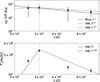 |
Fig. 5. Top panel: Break frequency resulting from the fit as a function of time. The expected behavior is overplotted with a solid line in the case of a wind environment and with dashed and dot-dashed lines in the case of ISM. The vertical shaded line represents the assumed deceleration time. Bottom panel: Peak flux in the spectra as a function of time. The expected behavior as a function of time for the wind environment is constant, while that for the ISM is plotted in dashed lines. |
Even in the case of a cocoon scenario, we expect a large density. In fact, the synchrotron self-absorption in a cocoon in ISM (Piran et al. 2013; Hotokezaka & Piran 2015) is given by
 (3)
(3)
at the deceleration time tdec. Here, E is the total kinetic energy of the ejecta at initial velocity β0. Assuming that, at tdec, νsa = 5 GHz, ϵe = ϵB = 0.1, E = 1049 erg, and p = 2, for a β0 = 0.5 the density has to be on the order of 102 cm−3.
3.2. Modeling all the EP241021a components
3.2.1. Early-time afterglow
As mentioned above, the slopes of the optical and X-ray light curves suggest a refreshed shocks scenario. We used the model by Sari & Mészáros (2000), where the source is assumed to eject mass with a range of Lorentz factors γ, with M(> γ)∝γ−s. The fast ejecta produces a forward shock (FS) when it reaches the material surrounding the collapse at the deceleration radius. As it reaches the fast ejecta, the slow ejecta produces the refreshing effect and a reverse shock (RS), which propagates inward. In a wind environment (ρ ∝ r−g with g = 2), the slopes of the forward and reverse shock light curves are a function of p and s (Sari & Mészáros 2000). The peak flux of the spectrum, its frequency (νm, in the assumption of slow cooling), and the cooling frequency νc, depend on the initial energy and the maximum Lorentz factor of the ejecta (E0 and γ0), on the density of the environment through A*, and on the microphysical parameters ϵe and ϵB.
As priors, we chose uniform distributions for each parameter, in particular: γ0 in [15, 100], E0 in [1048, 1051] ergs, ϵe and ϵB in [0.3, 0.001]. We fit the data up to ∼6 d (before the bump), including the optical and X-ray light curves, and the 5 GHz upper limit at 3.8 days. We fix the values of g = 2 (wind) and p. The latter was derived from the X-ray data in Section 2.2.1, where we find a photon index of Γ = 1.92 ± 0.22 before 6 d. Assuming the X-rays are above the synchrotron cooling frequency νc at such early times, this leads to a spectral slope β = Γ − 1 = 0.92 ± 0.2, and p = 1.85 ± 0.39. Since p > 2, we fix p = 2.
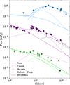 |
Fig. 6. EP241021a broadband light curve modeling. The dataset is shown as in Fig. 1, with the addition of the dark green upper limit at ∼89 d from XMM Newton, reported in Shu et al. (2025). The solid line represents the sum of an early refreshing phase (the wings of the jet, dot dashed line), the jet’s off-axis core (dotted line), and a cocoon (dashed line). In the optical band, the expected emission of SN1998bw (shaded black line) is also included in the sum. The cocoon emission is mainly relevant for the radio band. The optical light curve is represented in the plot, while the X-ray light curve has a peak flux of ∼2 × 10⁻⁸ mJy. |
The light curve fit is represented in Fig. 6, dot-dashed line, and Fig. B.1. The radio, optical, and X-ray data are fit with the blue, purple, and green curves, respectively. The fit is done only on the data before the bump, shown in Fig. B.1 by the vertical dashed line. In Fig. B.1, the solid line represents the sum of the contribution expected for the forward and reverse shocks, while the dotted and dashed lines represent the two components separately. The forward shock dominates the emission only at high energy. The fit easily explains the early part of the afterglow, before the bump. The parameters we find are reported in Table 2. The fastest ejecta with γ0 = 39 ( ) and E0 = 2.6 × 1049 erg (
 ), reach the external medium at a deceleration time of ∼10 sec. The observations in the optical and X-ray bands correspond to the time at which the ejecta with Lorentz factors between 7 and 9 reach the fast ejecta. Up to 6 days, during which this component dominates the emission, there is no evidence of a jet break; this implies a jet opening angle wider than 25 deg (Chevalier & Li 2000). Therefore, the beaming-corrected energy has a lower limit of 2.7 × 1048 erg.
Fit results for the broadband light curve.
Once all of the refreshing material reached the rest of the ejecta, the refreshing phase ended, and the afterglow returned to a standard light curve with increased energy. The shaded lines in Fig. B.1 after the vertical dashed line show the extrapolation of the model, assuming that the refreshing phase continues, with material with Lorentz factors of ∼2 reaching the deceleration radius at ∼5000 days. The fact that the refreshing ejecta are still relativistic at such late times is due to the decreasing density of the environment with distance, n ∝ r−2. Due to the bump, we are actually unable to identify the exact moment at which the energy injection stops. However, the X-ray upper limit at 89 d from Shu et al. (2025) suggests that the injection stops shortly after the bump, as early as 7 days, corresponding to Lorentz factors of ∼7. This model is represented with dot-dashed lines in Fig. B.1.
Considering that there is no sign of a jet break before the bump, it is likely that we observe a wide ejecta (as also found in Busmann et al. 2025; Yadav et al. 2025 with Lorentz factors in agreement with our γ0), on axis. Moreover, a γ0 ∼ 40 places this component at the low end of the γ0 distribution of long GRBs in a wind environment (Ghirlanda et al. 2018). Therefore, this ejecta is either a slow, baryon-loaded jet or a part of a structured jet. In the latter case, this wide component corresponds to the extended and less energetic wings (low-γ0), which surround an energetic and uniform jet core. We adopt this explanation in the rest of the paper, as it also explains the bump after 6 days, as we describe in the following section.
3.2.2. Re-brightening at 7 days
There is a clear re-brightening at ∼7 d, present both in the optical and X-rays. Here we discuss different explanations.
A re-brightening in the light curve can be caused by density inhomogeneities (overdensity) in the medium surrounding the star. An increase in the ambient density should be followed by a decrease in radio luminosity, arising from the increase in synchrotron self-absorption, which does not seem to be present. We also note that, if the X-rays are above the cooling frequency νc, they are not influenced by density (Kumar 2000; Freedman & Waxman 2001), and the re-brightening is expected mainly in the optical. However, this is not the case here, as at 8 d we find νc > 2.5 × 10¹⁷ Hz (see Fig. 3). The most compelling argument against density fluctuation is the fast rise of the bump, with a Δt/t ≈ 0.2, much shorter than expected in such a case, with Δt/t ≈ 1 (Nakar & Piran 2003; Nakar & Granot 2007; van Eerten et al. 2009; Gat et al. 2013).
The optical and X-ray bump is reminiscent of refreshed shocks, which we already introduced in Section 3.2.1. Indeed, this is the preferred explanation for this bump in Busmann et al. (2025). A fast re-brightening is expected if the slow ejecta, which catches up with the relativistic jet, is characterized by a single Lorentz factor (Piro et al. 1998, GRB 970508, as an example). Another clear example of a light curve with refreshed shocks is GRB 030329, which shows multiple components reaching the relativistic jet at different times, before and after the jet break (Granot et al. 2003). The fact that the shocks reach the relativistic material before or after the jet break time influences the timescale of the resulting bumps in the light curve. In particular, one expects that before the jet break, the bump rising time Δt should be on the order of t (Vlasis et al. 2011), instead, after the jet break Δt < t. In the case of EP241021a, Δt ∼ 1 d, while t ∼ 6 d, suggesting a post-jet break scenario. This, however, disagrees with the slope of the light curve before the bump, which does not show evidence of a jet break. For this reason, we do not prefer this explanation for the optical and X-ray bump.
The absolute peak magnitude of the optical bump is −21.5, consistent with fast blue optical transients (FBOTs, Drout et al. 2014). An FBOT was found associated with another EP event, EP240414a (Sun et al. 2025; van Dalen et al. 2025). However, their spectra are typically blue, which is not the case of the EP241021a, see also Busmann et al. (2025).
Finally, bumps in the optical light curves of GRBs are often identified as SNe. In this case, the rise time and the absolute magnitude are respectively too short and too bright to be explained as a SN, see Busmann et al. (2025) for an extended discussion.
After discarding all the scenarios above, we interpreted this bump as a signature of an off-axis jet. This modeling was already suggested for XRF 030723 (Butler et al. 2005), which has a fast bump in the optical light curve, hardly explained with a SN due to its short timescale (Huang et al. 2004; Fynbo et al. 2004). We used afterglowpy (Ryan et al. 2020, 2024) to model the light curve and, because of the short rise timescale, we assumed a top-hat jet, fixing the jet opening angle θc to 0.03 rad (1.7 deg), as also found in Huang et al. (2004). Moreover, we assumed a wind environment, as indicated by the early data (see Section 3.2.1). The fitted parameter and their priors are the following: the viewing angle θv in [0, π/2]; the isotropic equivalent kinetic energy of the jet E0 in [1051, 1055] ergs; the reference number density at a radius of 1017 cm in [10−1, 103] cm−3; the power law slope of the accelerated electrons p in [2,3], the fraction of energy in the accelerated electrons ϵe in [0.3, 0.001]; and the fraction of energy in the magnetic field ϵB in [0.3, 0.001].
The broadband fit is represented in Fig. 6. We assume that the refreshing phase in the jet wings described in Section 3.2.1 ends at 7 d, this fit is represented with dot-dashed lines. The dotted line represents the off-axis jet, which mainly contributes to the bump. The radio light curve is represented in blue in Fig. 6. As shown in our phenomenological analysis (Section 3.1), except for the early (t < 10 d) data, the main contribution is due to another radio component, the cocoon, which we introduce in Section 3.2.3.
Focusing on the early optical, X-ray, and radio data (t < 20 d), the overall light curve behavior is well described by the sum of the early refreshed shock phase, taking place in a wide ejecta (the jet wings) surrounding the jet core, and the Top Hat core itself, seen off-axis. For the off-axis Top Hat jet core, we find θv = 0.114 ± 0.004 rad, log(E0) = 54.51 ± 0.03, log(n0) = 1.11 ± 0.05,  , log(ϵe) = − 0.68 ± 0.10, and
  , see also Table 2 and the corner plot in Fig. B.3. The total beaming-corrected energy is 1.5 × 1051 erg. These parameters agree with studies of GRBs (Aksulu et al. 2022). The jet’s main contribution is at high frequencies. In Table 2 we report the value of A* instead of the reference density n0, to compare it with the refreshed shocks model. We find that the energetics of the two jet components (wings and core) is ∼5 orders of magnitude apart, with the off-axis core having an energetics in agreement with long GRBs (Aksulu et al. 2022). The other parameters, ϵe, ϵB are in agreement within the two components, even if they are not necessarily expected to be equal. Instead, we expect similar values for A*, which are in agreement within 2σ.
The late-time optical data points (t > 20 d) suggest a flattening in the light curve, which cannot be explained by the off-axis jet (dotted line). A natural way to account for it is by introducing a SN component, already associated with other XRFs (Bersier et al. 2006; Pian et al. 2006, as examples). In fact, adding the SN1998bw (at z = 0.75) contribution would perfectly fit the optical data after 20 days, as demonstrated in Fig. 6.
Busmann et al. (2025) discard a structured jet as explanation for this afterglow because of the too steep rise of the flux during the bump. However, even if our modeling confirms that the fast rise of the bump is not perfectly taken into account, we show that this scenario well catches the overall flux behavior.
3.2.3. Late-time radio afterglow
As demonstrated in Section 3.1, the radio afterglow after ∼10 d is described by a bell-shaped spectrum, which cannot explain the emission in the optical and X-rays. A self-absorbed radio spectrum characterizes also the emission expected from a SN Ic (Corsi et al. 2016). However, the EP241021a luminosity in the radio band exceeds by more than 1 order of magnitude the expected luminosity of a radio SN. Moreover, FBOTs also show self-absorbed radio spectra (Bright et al. 2022; Ho et al. 2019), but their luminosity at 9 GHz is ∼1028 erg s−1 Hz−1, nearly ∼2 orders of magnitude lower than EP241021a radio emission.
As mentioned in Section 3.1, we interpret the radio emission to be produced by a spherical ejecta, so-called cocoon (Cocoon I), which can be either nonrelativistic or mildly relativistic (γ ≲ 2), in a constant density environment (see Section 3.1). We used the afterglowpy cocoon model, in which we assumed that the ejecta is made by one single shell, with velocity u = βγ, total kinetic energy Etot, and mass
 (4)
(4)
where c is the velocity of light. The fitted parameters and the respective (all uniform) priors are the following: the velocity of the ejecta u in [0.1, 2]; the total kinetic energy Etot in [1048, 1052]; the density of the environment n0 in [10−3, 104]; the slope of the accelerated electron population p in [2,4]; the fraction of energy in the accelerated electrons ϵe in [0.3, 0.001]; and the fraction of energy in the magnetic field ϵB in [0.3, 0.001]. The prior bounds are inspired by Hotokezaka & Piran (2015), whose discussion, however, is mainly based on binary neutron star mergers. For this reason, we expand the parameter bounds regarding the energetics, the density and the mass of the ejecta.
The results are reported in the fourth column of Table 2, while the corner plot is in Fig. B.4. The fit is represented in Fig. 6 with dashed lines. The model fits well the radio data after 10 days, while the optical and X-ray emission do not influence the observed fluxes (the expected optical light curve is represented by the dashed purple line in the Figure, while the X-ray is not represented and reaches a peak flux of ∼2 × 10⁻⁸ mJy). The cocoon ejecta is mildly relativistic, in agreement with Shu et al. (2025), with a β = 0.73 ± 0.01,  and a mass of
  . The density of the environment is quite high, with a median value of 2.8 × 103 cm−3. Ejecta with γ ≥ 1.5 at 10 d is inferred also in Yadav et al. (2025), consistent with our findings for the cocoon. However, from a broad-band fit, they then identify these ejecta as a relativistic jet (Lorentz factor of 30–50), able to reproduce the X-ray, optical and radio afterglow (not including the bump). However, we note that this interpretation would result in a synchrotron self-absorption frequency νsa ≪ 1 GHz, which does not fit the steep break that we find in the radio spectrum at ν ∼ 4 GHz. Moreover, this model would not explain the early flat X-ray light curve exhibited by the EP-FXT data presented here (see Fig. 6 and Section 3.2.1).
3.2.4. ALMA component
In the radio spectrum at 70 days, there is clearly a second component (Cocoon II, see Fig. 4), peaking at ∼50 GHz and with a spectral shape again consistent with synchrotron self-absorption. We fit this emission with a second cocoon; the priors and parameters are the same as reported in Section 3.2.3. The results for the fit are written in Table 2, last column. This cocoon is slower than the cocoon described in Section 3.2.3, with Lorentz factor of  ,
,  and a mass of
  . The density of the environment is in agreement with the cocoon that produced the main radio afterglow, suggesting the same environment.
We focused on a scenario that envisages a complex jet structure and associated cocoon. However, we note that a double-peaked synchrotron spectrum can also emerge in a high-density medium, where the condition νc < νa holds (Gao et al. 2013). Under these circumstances, a thermal component arises, besides the broken power-law synchrotron (Ressler & Laskar 2017). This leads to a two-component (thermal and nonthermal) spectrum, with a peak at νa, originating from the thermal component of the electron population, and a second peak at νm. In this scenario, however, the synchrotron emission peaking at νm is expected to be broader than what we observe, with a spectral slope of 1/3 before the peak, which is inconsistent with the spectrum of EP241021a.
Another alternative explanation is that the second spectral peak arises from the reverse shock (Kobayashi et al. 2004; Gao et al. 2013), still under the regime νc < νa with νa > max(νm, νc). However, the detection of a refreshed shock emission at such late times appears highly improbable (Laskar et al. 2018, 2019). Finally, we find that in our cocoon models νc is much larger than νa, contrary to the condition required by these scenarios.
4. Discussion
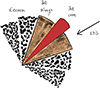 |
Fig. 7. Sketch of the proposed scenario for EP241021a. At small polar angles, a relativistic jet with a top-hat core and wide wings is produced, while at large polar angles, the jet is surrounded by a structured cocoon (with a mildly relativistic and nonrelativistic component). The observer’s line of sight lies within the wings of the jet. |
The physical modeling of EP241021a suggests that several components come into play, the complete spectral fit is represented in Fig. 8. The system at small polar angles is composed of one structured jet with an energetic top-hat core and external wider and low-Lorentz-factor wings, see a sketch in Fig. 7. Our line of sight is within the wings, but outside the collimated core. This results in the emission being dominated first by the wings (slow decay in optical and radio band), and later by the collimated core (bump in the optical and X-ray), once it enters our line of sight. The prompt emission in the soft X-rays is likely originated in the wide baryon-loaded wings, as it is also theorized in Busmann et al. (2025). We cannot rule out the presence of a SN; in fact, it would provide a natural explanation for the shallow decline of the optical light curve at late times (see also Busmann et al. 2025). The geometry of this system, with on-axis wide and less energetic wings and an off-axis core, could explain why previous analyses of the XRF afterglow population (D’Alessio et al. 2006; Gendre et al. 2007) found no compelling evidence for XRFs to originate from an off-axis jet. As in the EP241021a case, a less energetic and wider component could dominate the emission at early times, masking the typical rising light curve of off-axis GRBs.
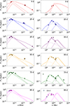 |
Fig. 8. EP241021a spectra at different times, up to 95 days. The broadband spectrum is represented in the first column, while a zoom of the radio spectrum is represented in the second column. The observation date is shown in the top right of each plot. The solid line represents the sum of all the components: the relativistic jet producing the optical and X-ray emission (in dotted line), the main cocoon emission producing the radio data (dashed lines), and the cocoon producing the ALMA data (dot-dashed lines). In the last two panels, the blue upper limit refers to the u-GMRT observation at ∼154 days, while the other data points refer to those taken at ∼95 days. |
The radio emission at ν < 20 GHz is produced by a spherical mildly relativistic ejecta, the cocoon, which is located at large polar angles (see Fig. 7). Possibly, this is a stratified cocoon with two different velocities, explaining the second spectral peak found at 70 days and ν > 20 GHz. The spectrum is self-absorbed, with a peak frequency (νsa) of ∼5 GHz. Such a high νsa suggests a high density, of 103 cm−3, which is in contrast with the lower density found by the jets.
Therefore, this system suggests an anisotropic medium. Taking as a reference a radius of 1017 cm, the cocoon expands in a constant density medium with ∼103 cm−3, while the two jets suggest a much lower 1 − 10 cm−3. The densities from the two jet components are in agreement with each other, as the jet wings have a wide constraint on the density, see Table 2. These differences can be explained by an anisotropic medium with higher densities at higher polar angles, shaped by the wind progenitor. This scenario agrees with the evidence of anisotropic winds in WR stars associated with their large rotational velocity (Shenar et al. 2019; Callingham et al. 2019). The slower, denser wind is ejected along the equatorial plane, where the cocoon is expanding, likely encountering a constant density termination shock produced by the denser wind interacting with the ISM. On the other hand, the faster, low-density component of the wind is ejected along the rotation axis, hence in the direction encountered by the relativistic jet.
After the collapse of a massive star, 3D hydrodynamical simulations predict the presence of a cocoon – with an inner mildly relativistic part and an outer nonrelativistic part – alongside a structured jet, where the wings represent a transition area between the energetic and relativistic core of the jet and the cocoon (Gottlieb et al. 2020; Harrison et al. 2018; Ito et al. 2015; Mizuta & Ioka 2013). In fact, such a jet-cocoon system has been proposed to explain other soft X-ray transients discovered by EP. EP240414a (Hamidani et al. 2025a; Zheng et al. 2025) shows optical re-brightening, interpreted with a nonthermal component: either an off-axis jet (Zheng et al. 2025) or a mildly relativistic cocoon (Hamidani et al. 2025b), followed by SN emission. The luminosity of the radio afterglow of this transient, produced by the mildly relativistic cocoon, is located between low-luminosity GRBs and cosmological GRBs, in agreement with our findings for EP241021a. Furthermore, a nonrelativistic cocoon is identified through a thermal spectrum in the optical at t < 1.2 d. In the case of EP241021a, observations start only later than ∼1 day, and thermal emission from the nonrelativistic cocoon identified in the high frequency radio band cannot be ruled out. EP240108a (Li et al. 2025; Eyles-Ferris et al. 2025; Rastinejad et al. 2025) shows a shallow decay in the optical afterglow, before showing re-brightening due to a SN at ∼10 d (Eyles-Ferris et al. 2025; Rastinejad et al. 2025), but there were no detections at radio and X-ray wavelengths. The early decaying phase is interpreted as the afterglow from a jet with a moderate Lorentz factor or as shock-cooling emission from a cocoon (Li et al. 2025).
Also in past GRBs, there is evidence of systems with a jet and a cocoon, such as in GRB 130925A, where X-ray thermal emission is detected (Piro et al. 2014), and GRB 160623A, where a cocoon produces the radio afterglow (Chen et al. 2020b). In general, multicomponent jets were found also in XRF 030723 (Huang et al. 2004), GRB030329 (Berger et al. 2003; Resmi et al. 2005), GRB 080413B (Filgas et al. 2011), GRB 221009A (Sato et al. 2023; Laskar et al. 2023; O’Connor et al. 2023).
5. Conclusions
We presented a comprehensive multiwavelength analysis of EP241021a, a soft X-ray transient detected by the Einstein Probe, interpreting its properties within the framework of XRFs. The prompt emission characteristics, along with the isotropic distribution and soft spectral peak, support the classification of EP241021a as an XRF.
Our observations reveal a complex, multicomponent afterglow, consistent with theoretical models involving structured jets and cocoon emissions. The optical and X-ray light curves at early times are best explained by wide-angled, low-Lorentz-factor structured wings, followed by the delayed emergence of the off-axis jet core. The radio afterglow is well modeled by two distinct cocoon components – mildly (at ν ≤ 20 GHz) and nonrelativistic (ν > 20 GHz) – implying a stratified outflow geometry.
Furthermore, our findings suggest significant asymmetry in the circumstellar medium, with a low-density region along the jet axis and denser material at wider angles, consistent with the wind structure of WR progenitors. This supports the theory that XRFs represent a softer and/or off-axis manifestation of long GRBs shaped by both viewing angles and explosion dynamics.
We find that the EP241021a emission aligns with a collapsar scenario. However, due to its complexity, other possible interpretations can be put forward, such as a complex tidal disruption event, proposed in Shu et al. (2025), or a catastrophic collapse or merger of a compact star system, which led to the formation of a millisecond magnetar, in Wu et al. (2025).
Thanks to its sensitivity and ability to detect soft X-ray energies, EP has revealed a landscape that remained hidden for years. As the number of XRFs continues to increase, it is possible that some or even all of these phenomena can eventually be explained by these multiple components interacting over various timescales. Crucially, studying these transients requires coordinated observations across multiple facilities and wavelengths. As demonstrated in this event, each energy band provides a piece of the story, and only by combining them can we gain a complete understanding of the system producing the observed transient.
Acknowledgments
The authors thank the anonymous referee for the useful comments. The authors also thank Bing Zhang for stimulating discussion. This work is based on data obtained with the Einstein Probe, a space mission supported by the Strategic Priority Program on Space Science of the Chinese Academy of Sciences, in collaboration with ESA, MPE and CNES (Grant No. XDA15310000, No. XDA15052100). We acknowledge support by the European Union Horizon 2020 programme under the AHEAD2020 project (grant agreement number 871158). This work has been also supported by ASI (Italian Space Agency) through the Contract no. 2019-27-HH.0 AJCT acknowledges support from the Spanish Ministry project PID2023-151905OB-I00 and Junta de Andalucía grant P20_010168 and from the Severo Ochoa grant CEX2021-001131-S funded by MCIN/AEI/10.13039/501100011033. MCG acknowledges support from the Spanish Ministry project PID2023-149817OB-C31. e-MERLIN is a National Facility operated by the University of Manchester at Jodrell Bank Observatory on behalf of STFC. This project has received funding from the European Union’s Horizon 2020 research and innovation programme under grant agreement No 101004719. Based on observations collected at the Centro Astronómico Hispano en Andalucía (CAHA) at Calar Alto, proposal 24B-2.2-012, operated jointly by Junta de Andalucía and Consejo Superior de Investigaciones Científicas (IAA-CSIC). Also based on observations made with the Gran Telescopio Canarias (GTC), installed at the Spanish Observatorio del Roque de los Muchachos of the Instituto de Astrofísica de Canarias, on the island of La Palma. The Australia Telescope Compact Array is part of the Australia Telescope National Facility (grid.421683.a), which is funded by the Australian Government for operation as a National Facility managed by CSIRO. We acknowledge the Gomeroi people as the traditional owners of the Observatory site. We thank the staff of the GMRT that made these observations possible. GMRT is run by the National Centre for Radio Astrophysics of the Tata Institute of Fundamental Research. This paper makes use of the following ALMA data: ADS/JAO.ALMA#2024.A.00019.T. ALMA is a partnership of ESO (representing its member states), NSF (USA) and NINS (Japan), together with NRC (Canada), NSTC and ASIAA (Taiwan), and KASI (Republic of Korea), in cooperation with the Republic of Chile. The Joint ALMA Observatory is operated by ESO, AUI/NRAO and NAOJ.
References
- Aksulu, M. D., Wijers, R. A. M. J., van Eerten, H. J., & van der Horst, A. J. 2022, MNRAS, 511, 2848 [NASA ADS] [CrossRef] [Google Scholar]
- Alam, S., Albareti, F. D., Allende Prieto, C., et al. 2015, ApJS, 219, 12 [Google Scholar]
- Aloy, M. A., Müller, E., Ibáñez, J. M., Martí, J. M., & MacFadyen, A. 2000, ApJ, 531, L119 [CrossRef] [Google Scholar]
- Aryan, A., Chen, T.-W., Yang, S., et al. 2025, arXiv e-prints [arXiv:2504.21096] [Google Scholar]
- Barraud, C., Olive, J.-F., Lestrade, J. P., et al. 2003, A&A, 400, 1021 [NASA ADS] [CrossRef] [EDP Sciences] [Google Scholar]
- Berger, E., Kulkarni, S. R., Pooley, G., et al. 2003, Nature, 426, 154 [NASA ADS] [CrossRef] [Google Scholar]
- Bersier, D., Fruchter, A. S., Strolger, L.-G., et al. 2006, ApJ, 643, 284 [NASA ADS] [CrossRef] [Google Scholar]
- Bi, X., Mao, J., Liu, C., & Bai, J.-M. 2018, ApJ, 866, 97 [NASA ADS] [CrossRef] [Google Scholar]
- Bochenek, A., & Perley, D. A. 2024a, GCN, 37869, 1 [Google Scholar]
- Bochenek, A., & Perley, D. A. 2024b, GCN, 37869, 1 [Google Scholar]
- Bochenek, A., & Perley, D. A. 2024c, GCN, 38030, 1 [Google Scholar]
- Bright, J. S., Margutti, R., Matthews, D., et al. 2022, ApJ, 926, 112 [NASA ADS] [CrossRef] [Google Scholar]
- Busmann, M., Gruen, D., O’Connor, B., Palmese, A., & Schmidt, M. 2024, GCN, 37877, 1 [Google Scholar]
- Busmann, M., O’Connor, B., Sommer, J., et al. 2025, A&A, 701, A225 [NASA ADS] [CrossRef] [EDP Sciences] [Google Scholar]
- Butler, N. R., Sakamoto, T., Suzuki, M., et al. 2005, ApJ, 621, 884 [Google Scholar]
- Callingham, J. R., Tuthill, P. G., Pope, B. J. S., et al. 2019, Nat. Astron., 3, 82 [Google Scholar]
- Campana, S., Mangano, V., Blustin, A. J., et al. 2006, Nature, 442, 1008 [NASA ADS] [CrossRef] [Google Scholar]
- Chakraborti, S., & Ray, A. 2011, ApJ, 729, 57 [Google Scholar]
- Chakraborti, S., Soderberg, A., Chomiuk, L., et al. 2015, ApJ, 805, 187 [NASA ADS] [CrossRef] [Google Scholar]
- Chandra, P., & Frail, D. A. 2012, ApJ, 746, 156 [NASA ADS] [CrossRef] [Google Scholar]
- Chen, Y., Cui, W., Han, D., et al. 2020a, in Space Telescopes and Instrumentation 2020: Ultraviolet to Gamma Ray, eds. J.-W. A. den Herder, S. Nikzad, & K. Nakazawa, SPIE Conf. Ser., 11444, 114445B [Google Scholar]
- Chen, W. J., Urata, Y., Huang, K., et al. 2020b, ApJ, 891, L15 [Google Scholar]
- Chen, J.-C., Urata, Y., & Huang, K. 2021, ApJ, 915, 46 [Google Scholar]
- Chevalier, R. A. 1998, ApJ, 499, 810 [NASA ADS] [CrossRef] [Google Scholar]
- Chevalier, R. A., & Li, Z.-Y. 2000, ApJ, 536, 195 [NASA ADS] [CrossRef] [Google Scholar]
- Corsi, A., Gal-Yam, A., Kulkarni, S. R., et al. 2016, ApJ, 830, 42 [Google Scholar]
- D’Alessio, V., Piro, L., & Rossi, E. M. 2006, A&A, 460, 653 [CrossRef] [EDP Sciences] [Google Scholar]
- Dermer, C. D., Chiang, J., & Mitman, K. E. 2000, ApJ, 537, 785 [Google Scholar]
- Drout, M. R., Chornock, R., Soderberg, A. M., et al. 2014, ApJ, 794, 23 [Google Scholar]
- Evans, P. A., Beardmore, A. P., Page, K. L., et al. 2007, A&A, 469, 379 [NASA ADS] [CrossRef] [EDP Sciences] [Google Scholar]
- Evans, P. A., Beardmore, A. P., Page, K. L., et al. 2009, MNRAS, 397, 1177 [Google Scholar]
- Eyles-Ferris, R. A. J., Jonker, P. G., Levan, A. J., et al. 2025, ApJ, 988, L14 [Google Scholar]
- Filgas, R., Krühler, T., Greiner, J., et al. 2011, A&A, 526, A113 [NASA ADS] [CrossRef] [EDP Sciences] [Google Scholar]
- Fontana, A., Dunlop, J. S., Paris, D., et al. 2014, A&A, 570, A11 [NASA ADS] [CrossRef] [EDP Sciences] [Google Scholar]
- Foreman-Mackey, D. 2016, J. Open Source Softw., 1, 24 [Google Scholar]
- Freeburn, J., Andreoni, I., Quirola-Vasquez, J., et al. 2024a, GCN, 37911, 1 [Google Scholar]
- Freeburn, J., Andreoni, I., & Carney, J. 2024b, GCN, 37942, 1 [Google Scholar]
- Freedman, D. L., & Waxman, E. 2001, ApJ, 547, 922 [Google Scholar]
- Fu, S. Y., Tinyanont, S., Anutarawiramkul, R., et al. 2024a, GCN, 37842, 1 [Google Scholar]
- Fu, S. Y., Zhu, Z. P., An, J., et al. 2024b, GCN, 37840, 1 [Google Scholar]
- Fynbo, J. P. U., Sollerman, J., Hjorth, J., et al. 2004, ApJ, 609, 962 [Google Scholar]
- Gao, H., Lei, W.-H., Wu, X.-F., & Zhang, B. 2013, MNRAS, 435, 2520 [CrossRef] [Google Scholar]
- Gat, I., van Eerten, H., & MacFadyen, A. 2013, ApJ, 773, 2 [Google Scholar]
- Gehrels, N. 1986, ApJ, 303, 336 [Google Scholar]
- Gendre, B., Galli, A., & Piro, L. 2007, A&A, 465, L13 [NASA ADS] [CrossRef] [EDP Sciences] [Google Scholar]
- Ghirlanda, G., Nappo, F., Ghisellini, G., et al. 2018, A&A, 609, A112 [NASA ADS] [CrossRef] [EDP Sciences] [Google Scholar]
- Giallongo, E., Ragazzoni, R., Grazian, A., et al. 2008, A&A, 482, 349 [NASA ADS] [CrossRef] [EDP Sciences] [Google Scholar]
- Goldstein, A., Cleveland, W. H., & Kocevski, D. 2023, Fermi Gamma-ray Data Tools: v2.0.0 [Google Scholar]
- Gottlieb, O., Nakar, E., & Bromberg, O. 2020, MNRAS, 500, 3511 [NASA ADS] [CrossRef] [Google Scholar]
- Granot, J., Panaitescu, A., Kumar, P., & Woosley, S. E. 2002, ApJ, 570, L61 [NASA ADS] [CrossRef] [Google Scholar]
- Granot, J., Nakar, E., & Piran, T. 2003, Nature, 426, 138 [Google Scholar]
- Granot, J., Ramirez-Ruiz, E., & Perna, R. 2005, ApJ, 630, 1003 [Google Scholar]
- Hamidani, H., Sato, Y., Kashiyama, K., et al. 2025a, ApJ, 986, L4 [Google Scholar]
- Hamidani, H., Ioka, K., Kashiyama, K., & Tanaka, M. 2025b, ApJ, 988, 30 [Google Scholar]
- Harrison, R., Gottlieb, O., & Nakar, E. 2018, MNRAS, 477, 2128 [NASA ADS] [CrossRef] [Google Scholar]
- Heise, J. 2003, AIP Conf. Proc., 662, 229 [Google Scholar]
- Higson, E., Handley, W., Hobson, M., & Lasenby, A. 2019, Stat. Comput., 29, 891 [Google Scholar]
- Ho, A. Y. Q., Phinney, E. S., Ravi, V., et al. 2019, ApJ, 871, 73 [NASA ADS] [CrossRef] [Google Scholar]
- Hotokezaka, K., & Piran, T. 2015, MNRAS, 450, 1430 [NASA ADS] [CrossRef] [Google Scholar]
- Hu, J. W., Wang, Y., He, H., et al. 2024, GCN, 37834, 1 [Google Scholar]
- Huang, Y. F., Dai, Z. G., & Lu, T. 2002, MNRAS, 332, 735 [NASA ADS] [CrossRef] [Google Scholar]
- Huang, Y. F., Wu, X. F., Dai, Z. G., Ma, H. T., & Lu, T. 2004, ApJ, 605, 300 [NASA ADS] [CrossRef] [Google Scholar]
- Ito, H., Matsumoto, J., Nagataki, S., Warren, D. C., & Barkov, M. V. 2015, ApJ, 814, L29 [Google Scholar]
- J-Jin, J., Mu, H. Y., F, Z., Sun, Y. G., & Mao, R. W. Y. M. 2024, GCN, 37892, 1 [Google Scholar]
- Kobayashi, S., Mészáros, P., & Zhang, B. 2004, ApJ, 601, L13 [Google Scholar]
- Koposov, S., Speagle, J., Barbary, K., et al. 2024, https://doi.org/10.5281/zenodo.12537467 [Google Scholar]
- Kumar, P. 2000, ApJ, 538, L125 [Google Scholar]
- Kumar, A., Maund, J. R., Sun, N. C., et al. 2024, GCN, 37875, 1 [Google Scholar]
- Laskar, T., Alexander, K. D., Berger, E., et al. 2018, ApJ, 862, 94 [NASA ADS] [CrossRef] [Google Scholar]
- Laskar, T., Eerten, H. v., Schady, P., et al. 2019, ApJ, 884, 121 [NASA ADS] [CrossRef] [Google Scholar]
- Laskar, T., Alexander, K. D., Margutti, R., et al. 2023, ApJ, 946, L23 [NASA ADS] [CrossRef] [Google Scholar]
- Lazzati, D. 2005, MNRAS, 357, 722 [NASA ADS] [CrossRef] [Google Scholar]
- Li, W. X., Xue, S. J., Andrews, M., et al. 2024, GCN, 37844, 1 [Google Scholar]
- Li, W. X., Zhu, Z. P., Zou, X. Z., et al. 2025, arXiv e-prints [arXiv:2504.17034] [Google Scholar]
- Liu, Y., Sun, H., Xu, D., et al. 2025, Nat. Astron., 9, 564 [Google Scholar]
- MacFadyen, A. I., & Woosley, S. E. 1999, ApJ, 524, 262 [NASA ADS] [CrossRef] [Google Scholar]
- MacFadyen, A. I., Woosley, S. E., & Heger, A. 2001, ApJ, 550, 410 [NASA ADS] [CrossRef] [Google Scholar]
- Margutti, R., Soderberg, A. M., Wieringa, M. H., et al. 2013, ApJ, 778, 18 [NASA ADS] [CrossRef] [Google Scholar]
- Margutti, R., Milisavljevic, D., Soderberg, A. M., et al. 2014, ApJ, 797, 107 [NASA ADS] [CrossRef] [Google Scholar]
- Mizuta, A., & Ioka, K. 2013, ApJ, 777, 162 [NASA ADS] [CrossRef] [Google Scholar]
- Moldon, J. 2021, Astrophysics Source Code Library [record ascl:2109.006] [Google Scholar]
- Moskvitin, A. S., Spiridonova, O. I., & GRB follow-up Team. 2024a, GCN, 37850, 1 [Google Scholar]
- Moskvitin, A. S., Spiridonova, O. I., & GRB follow-up Team. 2024b, GCN, 37910, 1 [Google Scholar]
- Moskvitin, A. S., Spiridonova, O. I., & GRB follow-up Team. 2024c, GCN, 37951, 1 [Google Scholar]
- Nakar, E., & Granot, J. 2007, MNRAS, 380, 1744 [Google Scholar]
- Nakar, E., & Piran, T. 2003, ApJ, 598, 400 [Google Scholar]
- O’Connor, B., Troja, E., Ryan, G., et al. 2023, Sci. Adv., 9, eadi1405 [CrossRef] [Google Scholar]
- Pan, Y., Kumar, B., Lin, W., et al. 2024, GCN, 37968, 1 [Google Scholar]
- Patel, M., Gompertz, B. P., O’Brien, P. T., et al. 2023, MNRAS, 523, 4923 [NASA ADS] [CrossRef] [Google Scholar]
- Pérez-Fournon, I., Sun, N. C., Li, W., et al. 2024, GCN, 37858, 1 [Google Scholar]
- Pian, E., Amati, L., Antonelli, L. A., et al. 1999, A&AS, 138, 463 [NASA ADS] [CrossRef] [EDP Sciences] [Google Scholar]
- Pian, E., Mazzali, P. A., Masetti, N., et al. 2006, Nature, 442, 1011 [Google Scholar]
- Piran, T., Nakar, E., & Rosswog, S. 2013, MNRAS, 430, 2121 [NASA ADS] [CrossRef] [Google Scholar]
- Piro, L., & Hurley, K. 2012, in Gamma-ray Bursts, eds. C. Kouveliotou, R. A. M. J. Wijers, & S. Woosley (Cambridge, UK: Cambridge University Press) [Google Scholar]
- Piro, L., Amati, L., Antonelli, L. A., et al. 1998, A&A, 331, L41 [NASA ADS] [Google Scholar]
- Piro, L., De Pasquale, M., Soffitta, P., et al. 2005, ApJ, 623, 314 [Google Scholar]
- Piro, L., Troja, E., Gendre, B., et al. 2014, ApJ, 790, L15 [NASA ADS] [CrossRef] [Google Scholar]
- Pugliese, G., Xu, D., Izzo, L., et al. 2024, GCN, 37852, 1 [Google Scholar]
- Quirola-Vasquez, J. A., Malesani, D. B., Levan, A. J., Bauer, F. E., & Jonker, P. G. 2024, GCN, 37930, 1 [Google Scholar]
- Ramirez-Ruiz, E., Celotti, A., & Rees, M. J. 2002, MNRAS, 337, 1349 [Google Scholar]
- Rastinejad, J. C., Levan, A. J., Jonker, P. G., et al. 2025, ApJ, 988, L13 [Google Scholar]
- Resmi, L., Ishwara-Chandra, C. H., Castro-Tirado, A. J., et al. 2005, A&A, 440, 477 [NASA ADS] [CrossRef] [EDP Sciences] [Google Scholar]
- Ressler, S. M., & Laskar, T. 2017, ApJ, 845, 150 [NASA ADS] [CrossRef] [Google Scholar]
- Rhoads, J. E. 2003, ApJ, 591, 1097 [Google Scholar]
- Ror, A. K., Gupta, A., Tripathi, T., Pandey, S. B., & Mishra, K. 2024, GCN, 37845, 1 [Google Scholar]
- Ryan, G., Eerten, H. v., Piro, L., & Troja, E. 2020, ApJ, 896, 166 [CrossRef] [Google Scholar]
- Ryan, G., van Eerten, H., Troja, E., et al. 2024, ApJ, 975, 131 [Google Scholar]
- Sakamoto, T., Hullinger, D., Sato, G., et al. 2008, ApJ, 679, 570 [Google Scholar]
- Salafia, O. S., Barbieri, C., Ascenzi, S., & Toffano, M. 2020, A&A, 636, A105 [NASA ADS] [CrossRef] [EDP Sciences] [Google Scholar]
- Sari, R., & Mészáros, P. 2000, ApJ, 535, L33 [NASA ADS] [CrossRef] [Google Scholar]
- Sari, R., Piran, T., & Narayan, R. 1998, ApJ, 497, L17 [Google Scholar]
- Sari, R., Piran, T., & Halpern, J. P. 1999, ApJ, 519, L17 [NASA ADS] [CrossRef] [Google Scholar]
- Sato, Y., Murase, K., Ohira, Y., & Yamazaki, R. 2023, MNRAS, 522, L56 [NASA ADS] [CrossRef] [Google Scholar]
- Schneider, B., & Adami, C. 2024, GCN, 38022, 1 [Google Scholar]
- Shenar, T., Sablowski, D. P., Hainich, R., et al. 2019, A&A, 627, A151 [NASA ADS] [CrossRef] [EDP Sciences] [Google Scholar]
- Shu, X., Yang, L., Yang, H., et al. 2025, ApJ, 990, L29 [Google Scholar]
- Soderberg, A. M., Kulkarni, S. R., Nakar, E., et al. 2006, Nature, 442, 1014 [CrossRef] [Google Scholar]
- Soderberg, A. M., Chakraborti, S., Pignata, G., et al. 2010, Nature, 463, 513 [NASA ADS] [CrossRef] [Google Scholar]
- Speagle, J. S. 2020, MNRAS, 493, 3132 [Google Scholar]
- Starling, R. L. C., Wiersema, K., Levan, A. J., et al. 2011, MNRAS, 411, 2792 [NASA ADS] [CrossRef] [Google Scholar]
- Sun, H., Li, W. X., Liu, L. D., et al. 2025, Nat. Astron., 9, 1073 [Google Scholar]
- Svinkin, D., Frederiks, D., Lysenko, A., et al. 2024, GCN, 38034, 1 [Google Scholar]
- The CASA Team, Bean, B., Bhatnagar, S., et al. 2022, PASP, 134, 114501 [NASA ADS] [CrossRef] [Google Scholar]
- Urata, Y., Huang, K., Yamazaki, R., & Sakamoto, T. 2015, ApJ, 806, 222 [NASA ADS] [CrossRef] [Google Scholar]
- van Dalen, J. N. D., Levan, A. J., Jonker, P. G., et al. 2025, ApJ, 982, L47 [Google Scholar]
- van Eerten, H. J., Meliani, Z., Wijers, R. A. M. J., & Keppens, R. 2009, MNRAS, 398, L63 [Google Scholar]
- Vlasis, A., van Eerten, H. J., Meliani, Z., & Keppens, R. 2011, MNRAS, 415, 279 [NASA ADS] [CrossRef] [Google Scholar]
- Watson, D., Hjorth, J., Levan, A., et al. 2004, ApJ, 605, L101 [Google Scholar]
- Willingale, R., & Mészáros, P. 2017, Space Sci. Rev., 207, 63 [NASA ADS] [CrossRef] [Google Scholar]
- Woosley, S. E. 1993, ApJ, 405, 273 [Google Scholar]
- Wu, G.-L., Yu, Y.-W., Liu, L.-D., et al. 2025, EP241021a: A Catastrophic Collapse/merger of Compact Star Binary Leading to the Formation of a Remnant Millisecond Magnetar? [Google Scholar]
- Yadav, M., Troja, E., Ricci, R., et al. 2025, arXiv e-prints [arXiv:2505.08781] [Google Scholar]
- Yamazaki, R., Ioka, K., & Nakamura, T. 2002, ApJ, 571, L31 [NASA ADS] [CrossRef] [Google Scholar]
- Yoon, S.-C., & Langer, N. 2005, A&A, 443, 643 [NASA ADS] [CrossRef] [EDP Sciences] [Google Scholar]
- Yuan, W., Zhang, C., Chen, Y., & Ling, Z. 2022, The Einstein Probe Mission (Singapore: Springer Nature), 1 [Google Scholar]
- Yuan, W., Dai, L., & Feng, H. 2025, Sci. China Phys. Mech. Astron., 68, 239501 [Google Scholar]
- Zhang, B., & Mészáros, P. 2002, ApJ, 581, 1236 [Google Scholar]
- Zhang, W., Woosley, S. E., & MacFadyen, A. I. 2003, ApJ, 586, 356 [CrossRef] [Google Scholar]
- Zheng, W., Brink, T. G., Filippenko, A. V., Yang, Y., & KAIT GRB Team 2024, GCN, 38294, 1 [Google Scholar]
- Zheng, J.-H., Zhu, J.-P., Lu, W., & Zhang, B. 2025, ApJ, 985, 21 [Google Scholar]
Appendix A: Observations
EP-FXT observation log and flux measurements.
Optical observations of EP241021a.
Radio observations of EP241021a.
Appendix B: Corner plots and additional figures
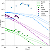 |
Fig. B.1. EP241021a broadband light curve. The dashed line represents the contribution of the RS, the dotted line represents the contribution of the FS, while the solid line represents the sum of FS and RS. The FS and RS are superimposed in the optical and X-ray bands. The data points before the vertical dashed line are fit, and the model following that is an interpolation, assuming that the refreshing phase continues up to 5 × 10³ days. The dot-dashed line represents the model interpolation when the refreshing phase ends at 10 days. The dark green X-ray upper limit at 89 d is derived from Shu et al. 2025. |
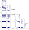 |
Fig. B.2. Corner plot of the early-time (t ≤ 6d) light curve fit using the refreshed shocks model. The dashed lines in the 1D histograms represent the 16th and 84th percentiles. The parameter values are indicated as median, 16th, and 84th percentiles. |
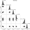 |
Fig. B.3. Corner plot of the off-axis top-hat jet. The dashed lines in the 1D histograms represent the 16th and 84th percentiles. The parameter values are indicated as median, 16th, 50th, and 84th percentiles. |
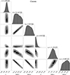 |
Fig. B.4. Corner plot of the cocoon fitting the radio data. The dashed lines in the 1D histograms represent the 16th and 84th percentiles. The parameter values are indicated as median, 16th, 50th, and 84th percentiles. |
All Tables
All Figures
|
Fig. 1. EP241021a broadband light curve. FXT observations are represented with green data points; optical observations are represented in shades of purple and pink; and radio data are represented in shades of blue. Inverted triangles indicate upper limits. The optical data represented with circles are taken from the literature (Busmann et al. 2025, 2024; Aryan et al. 2025; Fu et al. 2024a,b; Li et al. 2024; J-Jin et al. 2024; Pan et al. 2024; Ror et al. 2024; Kumar et al. 2024; Bochenek & Perley 2024a,b,c; Freeburn et al. 2024a,b; Quirola-Vasquez et al. 2024; Moskvitin & Spiridonova 2024a,b,c; Schneider & Adami 2024). The solid black lines and shaded-colored regions represent the best fit and the 500 best likelihood fits of the data using power law models. |
| In the text | |
|
Fig. 2. Left panel: X-ray luminosities in the 0.3–10 keV band of Swift-detected GRBs (Evans et al. 2007, 2009). Right panel: Radio afterglow luminosities at 9 GHz of the GRB catalog presented in Chandra & Frail (2012). EP241021a is represented in magenta stars, while low-luminosity GRBs, such as GRB 060218 (Campana et al. 2006; Soderberg et al. 2006), GRB 100316D (Starling et al. 2011; Margutti et al. 2013), GRB 980425 (Pian et al. 1999), and GRB 031203 (Watson et al. 2004) are represented with light blue, yellow, light red, and green squares, respectively, in both panels. |
| In the text | |
|
Fig. 3. EP241021a broadband spectrum at ∼8 d (top panel) and ∼25 d (bottom panel). In the top panel, the solid lines represent a fit of two broken power law models. In the bottom panel, the solid line represents the sum of the radio and optical components, represented with dotted and dashed lines, respectively. |
| In the text | |
|
Fig. 4. EP241021a radio spectrum at 70 days. The 5 sigma upper limits from uGMRT are represented as triangles; ATCA observations are represented with dots; and ALMA observations are represented with stars. The spectra are fit with a broken power-law model, the colored regions represent the 500 highest-likelihood fits, while the black line represents the best fit. |
| In the text | |
|
Fig. 5. Top panel: Break frequency resulting from the fit as a function of time. The expected behavior is overplotted with a solid line in the case of a wind environment and with dashed and dot-dashed lines in the case of ISM. The vertical shaded line represents the assumed deceleration time. Bottom panel: Peak flux in the spectra as a function of time. The expected behavior as a function of time for the wind environment is constant, while that for the ISM is plotted in dashed lines. |
| In the text | |
|
Fig. 6. EP241021a broadband light curve modeling. The dataset is shown as in Fig. 1, with the addition of the dark green upper limit at ∼89 d from XMM Newton, reported in Shu et al. (2025). The solid line represents the sum of an early refreshing phase (the wings of the jet, dot dashed line), the jet’s off-axis core (dotted line), and a cocoon (dashed line). In the optical band, the expected emission of SN1998bw (shaded black line) is also included in the sum. The cocoon emission is mainly relevant for the radio band. The optical light curve is represented in the plot, while the X-ray light curve has a peak flux of ∼2 × 10⁻⁸ mJy. |
| In the text | |
|
Fig. 7. Sketch of the proposed scenario for EP241021a. At small polar angles, a relativistic jet with a top-hat core and wide wings is produced, while at large polar angles, the jet is surrounded by a structured cocoon (with a mildly relativistic and nonrelativistic component). The observer’s line of sight lies within the wings of the jet. |
| In the text | |
|
Fig. 8. EP241021a spectra at different times, up to 95 days. The broadband spectrum is represented in the first column, while a zoom of the radio spectrum is represented in the second column. The observation date is shown in the top right of each plot. The solid line represents the sum of all the components: the relativistic jet producing the optical and X-ray emission (in dotted line), the main cocoon emission producing the radio data (dashed lines), and the cocoon producing the ALMA data (dot-dashed lines). In the last two panels, the blue upper limit refers to the u-GMRT observation at ∼154 days, while the other data points refer to those taken at ∼95 days. |
| In the text | |
|
Fig. B.1. EP241021a broadband light curve. The dashed line represents the contribution of the RS, the dotted line represents the contribution of the FS, while the solid line represents the sum of FS and RS. The FS and RS are superimposed in the optical and X-ray bands. The data points before the vertical dashed line are fit, and the model following that is an interpolation, assuming that the refreshing phase continues up to 5 × 10³ days. The dot-dashed line represents the model interpolation when the refreshing phase ends at 10 days. The dark green X-ray upper limit at 89 d is derived from Shu et al. 2025. |
| In the text | |
|
Fig. B.2. Corner plot of the early-time (t ≤ 6d) light curve fit using the refreshed shocks model. The dashed lines in the 1D histograms represent the 16th and 84th percentiles. The parameter values are indicated as median, 16th, and 84th percentiles. |
| In the text | |
|
Fig. B.3. Corner plot of the off-axis top-hat jet. The dashed lines in the 1D histograms represent the 16th and 84th percentiles. The parameter values are indicated as median, 16th, 50th, and 84th percentiles. |
| In the text | |
|
Fig. B.4. Corner plot of the cocoon fitting the radio data. The dashed lines in the 1D histograms represent the 16th and 84th percentiles. The parameter values are indicated as median, 16th, 50th, and 84th percentiles. |
| In the text | |
Current usage metrics show cumulative count of Article Views (full-text article views including HTML views, PDF and ePub downloads, according to the available data) and Abstracts Views on Vision4Press platform.
Data correspond to usage on the plateform after 2015. The current usage metrics is available 48-96 hours after online publication and is updated daily on week days.
Initial download of the metrics may take a while.