© The Authors 2025

1. Introduction

In the classical scenario, a tidal disruption event (TDE; see, e.g., Rees 1988; Phinney 1989; for a recent review Rossi et al. 2021 and references therein) is an extreme phenomenon in which a star orbiting around a massive black hole (BH) is shred apart by its tides. The aftermath of the disruption is visible thanks to luminous (possibly super-Eddington) flares produced by accretion of the stellar debris onto the BH. Since the 1990s, we have detected these events through different wavelengths of the electromagnetic spectrum (see, e.g., recent reviews by van Velzen et al. 2020; Saxton et al. 2021 and references therein) and this number is expected to increase significantly in the near future thanks to upcoming sensitive detectors (Gomez et al. 2023), such as the Rubin Observatory Legacy Survey of Space and Time (LSST; Ivezić et al. 2019) and the Ultraviolet Transient Astronomy Satellite (ULTRASAT; Shvartzvald et al. 2024).

Lately, there has also been growing interest in a distinct class of TDEs, in which the star survives the first passage at the pericenter and undergoes multiple orbits before complete disruption (see e.g., Bortolas et al. 2023). The interest in these sources is also motivated by a possible link to recently observed quasiperiodic eruptions (QPEs; Linial & Metzger 2023), which still lack a widely accepted explanation (see, e.g., Franchini et al. 2023, for an alternative model).

Tidal disruption events are also expected to produce gravitational waves (GWs) in the low-frequency regime (millihertz-decihertz). Previous works (Kobayashi et al. 2004; Toscani et al. 2020; Pfister et al. 2022; Toscani et al. 2022, 2023) have already explored these signals, generally concluding that while LISA (Colpi et al. 2024) – the first GW space-based detector, set to launch in 2035 – is unlikely to observe these events, the situation will significantly improve with potential future interferometers optimized to the decihertz frequency band.

In this paper, we refine the estimates for future space-based gravitational observatories of both TDE detection rates, as well as of the GW background (GWB) from these sources, building on previous works by Toscani et al. (2020) and Pfister et al. (2022). First, we improve the strain estimate accounting for all harmonics contributing to the GW emission, following the formalism for parabolic encounters presented in Berry & Gair (2010). Second, we extend this study by incorporating a population of repeated partial disruptions, based on the model proposed in Broggi et al. (2024), to make the analysis more comprehensive. This scenario could be particularly intriguing from a GW perspective, as repeated passages of the star around the BH allow for the accumulation of the signal-to-noise ratio (S/N), potentially improving its detectability compared to complete disruptions, which feature, by definition, one single passage. For clarity, we introduce the following terminology: full TDEs (fTDEs), referring to classic stellar disruptions, and repeated partial TDEs (rpTDEs), describing the scenario in which the star undergoes multiple orbits around the BH.

The structure of the paper is the following. In Sections 2 and 3 we illustrate the calculations for fTDEs and rpTDEs respectively, computing the strain of individual events and the overall GWB. In Section 4 we discuss our findings and compare them to previous studies, and finally in Section 5 we draw our conclusions. In this work, we consider a ΛCDM model with H₀ = 70 km/s/Mpc and Ω_m = 0.3; we refer to the gravitational constant, the speed of light in vacuum, solar mass, and radius as G, c, M_⊙, and R_⊙ respectively.

2. Full disruptions

Before diving into calculations, we shall introduce some key concepts of dynamics of dense stellar systems surrounding a massive BH. In particular, we shall introduce the loss cone and illustrate the difference between full and empty loss cone regimes, which helps connect stellar dynamics to the nature of TDEs.

The loss cone (Frank & Rees 1976, recent review by Stone et al. 2020) is the region in the (specific) angular momentum and energy space where stars can pass close enough to the BH to be disrupted or captured. The fTDEs occur in the full loss cone regime (also referred to as the pinhole regime), where stars take large angular momentum steps over the orbital period and are scattered in and out of the loss cone within subsequent pericenter passages. This is the typical scenario of stars weakly bound to the BH, approaching almost radial orbits. If they are inside the loss cone at the pericenter, a full disruption happens. On the other hand, stars deeply bound to BH typically fall in the empty loss cone regime, where they need many orbital revolutions to change significantly their angular momentum, so that they graze the loss cone and their disruption is gradual. Hence, in this regime we have rpTDEs.

To be more quantitative, we can introduce the dimensionless parameter

$$\begin{array}{c}\hfill q={\left(\frac{\mathrm{\Delta }J}{J_{\mathrm{lc}}}\right)}^2,\end{array}$$(1)

where ΔJ is the step in the angular momentum and J_lc = (2GM_•R_p)^1/2 is the angular momentum at the surface of the loss cone, M_• being the BH mass and R_p the stellar pericenter. If q > 1, we are in the pinhole regime, while for q < 1 the empty loss cone regime holds. In the rest of this section, we analyze fTDEs.

2.1. Two examples

To get an order of magnitude idea of the GW signals we expect from these sources, we started by considering two examples¹: (i) a fTDE of a MS star with mass M_* = 0.1 M_⊙, destroyed by a BH of size M_• = 4 × 10⁶ M_⊙, and (ii) a fTDE of a WD with mass M_* = 0.5 M_⊙ and BH M_∙ = 10³ M_⊙. We examined two possible source distances: 8 kpc (the distance of the Galactic center of the Milky Way) and 1 Mpc (about the size of the Local Group of galaxies).

Considering that $|\stackrel{\sim }{h}(f)|$ is the Fourier transform of the GW strain, the inclination-polarization averaged characteristic strain reads

$$\begin{array}{c}\hfill h_{\mathrm{c}}^2=4{|\stackrel{\sim }{h}(f)|}^2{f}^2=\frac{G}{{\pi }^2{c}^3{\chi }^2}\frac{\mathit{dE}}{\mathit{df}},\end{array}$$(2)

where χ is the comoving distance (Hogg 1999). For the GW energy spectrum, dE/df, we used the expression for parabolic encounters illustrated in Berry & Gair (2010)

$$\begin{array}{c}\hfill \frac{\mathrm{d}E}{\mathrm{d}f}=\frac{4{\pi }^2{G}^3}{5c^5}\frac{M_{\bullet }^2{M}_{\ast }^2}{R_{\mathrm{p}}^2}\ell \left(\frac{f}{f_{\mathrm{c}}}\right),\end{array}$$(3)

with ℓ(f/f_c) containing the contributions from all the harmonics and f_c being the Keplerian frequency of the circular orbit with a radius equal to the stellar pericenter, R_p.

The S/N for a GW is given by (Maggiore 2008)

$$\begin{array}{c}\hfill {\text{S/N}}^2=4{\displaystyle {\int }_0^{\infty }}\mathrm{d}f\frac{|\stackrel{\sim }{h}{(f)|}^2}{S_n(f)},\end{array}$$(4)

where S_n(f) is the sky-averaged power spectral density (PSD) of the instrument. In this work, we consider two reference detectors: (i) LISA, assuming a mission duration of 10 years (Colpi et al. 2024), and (ii) an optimal model for the decihertz observatory (DO; in particular we refer to the instrument labeled as DO-optimal in Arca Sedda et al. 2020).

In Fig. 1, we plot h_c with respect to the noise amplitudes $(\sqrt{f{S}_{\mathrm{n}}})$ of both instruments, and we show that this signal is potentially detectable. In fact, the MS star emission could be seen by LISA (S/N ∼ 193) and also by DO (S/N ∼ 91) within our Galaxy²; however, it becomes undetectable to both instruments once the source is located outside the Milky Way. Instead for the WD, since the signal peaks around 0.1 Hz where DO is particularly sensitive, it can be seen by this instrument with a relatively high S/N (∼47) even at a distance of 1 Mpc. This is not the case for LISA, whose sensitivity is insufficient to detect the signal beyond a few kiloparsecs.

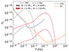Fig. 1. GW signal from a fTDE of a 0.1 M⊙ MS star disrupted by a 4 × 106 M⊙ BH (gray lines) and GW signal from a fTDE of a WD of 0.5 M⊙ disrupted by a 103 M⊙ BH (red lines). We consider two possible source distances: 8 kpc (dashed lines) and 1 Mpc (dash-dotted lines). In blue and orange, we plot the noise amplitudes of LISA and DO, respectively.

These estimates alone do not really inform us about the detectability of these sources. To understand whether they can be observed, we need to take into account the effective number of TDEs occurring in the Universe, as we illustrate in the following paragraphs.

2.2. Main-sequence stars: Individual detection rates

The rate of detected MS-fTDEs per bin of redshift z, BH mass M_•, stellar mass M_*, and pericenter R_p can be estimated as (Toscani et al. 2020; Pfister et al. 2022)

$$\begin{array}{cc}\hfill {\dot{N}}_{\det }^{\mathrm{fTDEs}}=& {\displaystyle \int \mathrm{d}}z{\displaystyle \int \mathrm{d}}{M}_{\bullet }{\displaystyle \int \mathrm{d}}{M}_{\ast }{\displaystyle \int \mathrm{d}}{R}_{\mathrm{p}}\hfill \\ \hfill & \frac{d^2\mathrm{\Gamma }(M_{\bullet })}{\mathrm{d}{M}_{\ast }\mathrm{d}{R}_{\mathrm{p}}}\times \frac{4\pi c{\chi }^2(z)}{H(z)}\times \frac{\mathrm{\Phi }(M_{\bullet },z)}{1+z}\times \mathrm{\Theta }(z,M_{\bullet },M_{\ast },R_{\mathrm{p}}).\hfill \end{array}$$(5)

The first term on the right-hand side of Eq. (5) is the differential TDE rate per galaxy, which we express as

$$\begin{array}{c}\hfill \frac{d^2\mathrm{\Gamma }(M_{\bullet })}{\mathrm{d}{M}_{\ast }\mathrm{d}{R}_{\mathrm{p}}}=\mathrm{\Gamma }(M_{\bullet })\mathcal{F}(M_{\bullet })\varphi (M_{\ast })\psi (R_{\mathrm{p}}).\end{array}$$(6)

Γ(M_•) is the TDE rate as a function of the BH mass, which we take from the recent work by Chang et al. (2025)

$$\begin{array}{c}\hfill \mathrm{\Gamma }(M_{\bullet })=\{\begin{array}{c}1.2\times {10}^{-4}{\text{yr}}^{-1}{\left(\frac{M_{\bullet }}{{10}^6{\text{M}}_{\odot }}\right)}^{0.9}{M}_{\bullet }\le {10}^6{\text{M}}_{\odot },\hfill \\ 1.2\times {10}^{-4}{\text{yr}}^{-1}{\left(\frac{M_{\bullet }}{{10}^6{\text{M}}_{\odot }}\right)}^{-0.9}{M}_{\bullet }>{10}^6{\text{M}}_{\odot }.\hfill \end{array}\end{array}$$(7)

ℱ(M_•) is the fraction of TDEs occurring in the pinhole regime (Stone & Metzger 2016, Eq. 29). ψ(R_p) is the uniform pericenter distribution (in agreement with loss cone theory). ϕ(M_*) is the Kroupa initial stellar mass function (Kroupa 2001),

$$\begin{array}{c}\hfill \varphi (M_{\ast })=\mathcal{N}\{\begin{array}{c}{M_{\ast }}^{-0.3}{M}_{\ast }\le 0.08{\text{M}}_{\odot },\hfill \\ {M_{\ast }}^{-1.3}0.08{\text{M}}_{\odot }<M_{\ast }\le 0.5{\text{M}}_{\odot },\hfill \\ {M_{\ast }}^{-2.3}0.5{\text{M}}_{\odot }<M_{\ast }\le 1{\text{M}}_{\odot },\hfill \\ {M_{\ast }}^{-2.7}{M}_{\ast }>1{\text{M}}_{\odot },\hfill \end{array}\end{array}$$(8)

where the constant, 𝒩, is chosen to have a continuous function, normalized on the interval (0, ∞). Φ(M_•, z) is the BH mass function that, following Pfister et al. (2022), we model as a redshift-dependent double Schechter function. The function parameters were obtained by fitting the galaxy mass function of the COSMOS field (Eq. 4 and Table I from Davidzon et al. 2017) and then by converting the galaxy mass into the central BH mass using the relation by Reines & Volonteri (2015). Finally, Θ is a step function, and is 1 if the gravitational signal from the TDE with z, M_•, M_*, R_p is above the threshold, and 0 otherwise.

In this calculation, we considered the following ranges for the variables:

• 0 ≲ z ≤ 3;

• 10⁴ M_⊙ ≤ M_∂ ≤ 10⁷ M_⊙;

• 0.1 M_⊙ ≤ M_* ≤ 1 M_⊙

• R_sch(M_•) ≤ R_p ≤ R_t(M_•,M_*), with R_sch the Schwarzschild radius of the BH and R_t the tidal radius.

The result is illustrated in Fig. 2, where we plot the detection rates as functions of the S/N thresholds for LISA (blue curve) and DO (orange curve). The dashed horizontal black line is one detection in 10 years. We see that while for LISA no detections of these events are expected, the situation is much better for DO. In this case, these sources could reach S/Ns of up to ∼10, with the number of detectable events varying from tens to hundreds, depending sensitively on the detection criteria adopted.

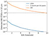Fig. 2. Detection rates of MS-fTDEs plotted for different S/N thresholds. The blue curve was calculated considering LISA as the detector, while the orange curve was obtained considering DO. The observation time for both instruments is assumed to be 10 years. The dashed black line is one event over 10 years.

2.3. Main-sequence stars: The background

The GW signal from the entire population of MS-fTDEs can be expressed as (Phinney 2001; Toscani et al. 2020)

$$\begin{array}{c}\hfill h_{\mathrm{c},\mathrm{pop}}^2=\frac{G}{c^3{\pi }^2}\times \frac{1}{f}\times {\displaystyle {\int }_0^{\infty }}\mathrm{d}z\frac{1}{{\chi }^2}\frac{\mathrm{d}{\dot{N}}^{\mathrm{tde}}}{\mathrm{d}z}\left(\frac{\mathrm{d}E}{\mathrm{d}f}\right),\end{array}$$(9)

with

$$\begin{array}{cc}\hfill \frac{\mathrm{d}{\dot{N}}^{\mathrm{tde}}}{\mathrm{d}z}\frac{\mathrm{d}E}{\mathrm{d}f}=& {\displaystyle \int \mathrm{d}}{M}_{\bullet }{\displaystyle \int \mathrm{d}}{M}_{\ast }{\displaystyle \int \mathrm{d}}{R}_{\mathrm{p}}\frac{d^4{\dot{N}}^{\mathrm{fTDEs}}}{\mathrm{d}z\mathrm{d}{M}_{\bullet }\mathrm{d}{M}_{\ast }\mathrm{d}{R}_{\mathrm{p}}}\hfill \\ \hfill & \times \frac{4{\pi }^2{G}^3}{5c^5}\frac{M_{\bullet }^2{M}_{\ast }^2}{R_{\mathrm{p}}^2}\ell \left(\frac{f}{f_{\mathrm{c}}}\right),\hfill \end{array}$$(10)

where the differential rate is the same as the integrand in Eq. (5) without the Θ term, since now we also want to include the sources below the threshold of detectability.

The result is illustrated in Fig. 3, where the magenta curve represents the background. Compared to the previous plots, here we also include a third observatory, μAres (Sesana et al. 2021), mainly as a reference given that this part of the frequency window (0.0001–0.001 Hz) will be heavily dominated by backgrounds from different astrophysical sources (Perego et al. in prep.). The plot shows that the signal lies orders of magnitude below the sensitivity curves of the three considered instruments. Nevertheless, the most informative way to assess its detectability is by computing its S/N, accounting for the observation time of the instrument. Following Eq. (7) of Sesana(2016), assuming T = 10 years and γ = 1, we get an S/N smaller than 1 in all cases, meaning that the signal will remain undetectable for the future space-based detectors considered in this study.

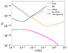Fig. 3. MS-fTDEs background (magenta curve) plotted with respect to the sensitivity curves of LISA (blue line), DO (orange line), and μAres (black line).

Finally, it is also worth noting that the signal is much lower than expected in Toscani et al. (2020). However, a direct comparison is not straightforward due to differences in the integration limits adopted in the two calculations. To address this, in Sect. 4, we carry out a detailed analysis to actually understand the origin of the difference between the two estimates.

2.4. White dwarfs: Individual detection rates

We now focus on the case of WD-fTDEs. This scenario is intriguing since, as has already been pointed out in Toscani et al. (2020), due to their compactness they generate gravitational signals comparable in magnitude to those produced by MS stars (cf. Fig. 1), although the BHs involved in the disruption are smaller³.

Here in particular we distinguish between two classes of events, involving WDs disrupted by different populations of BHs: (i) intermediate-mass BHs in the center of dwarf galaxies and (ii) intermediate-mass BHs residing in globular clusters (GCs). For case (i) the rate of detected WD-fTDEs is the same as in Eq. (5) apart from the differential TDE rate per galaxy, which reads

$$\begin{array}{c}\hfill \frac{d^2\mathrm{\Gamma }(M_{\bullet })}{\mathrm{d}{M}_{\ast }\mathrm{d}{R}_{\mathrm{p}}}=\mathrm{\Gamma }(M_{\bullet })\mathcal{F}(M_{\bullet })\delta (M_{\ast })\psi (R_{\mathrm{p}}).\end{array}$$(11)

The stellar mass distribution is replaced with a δ function, since we consider a WD population monochromatic in mass (with M_* = 0.5 M_⊙, R_* = 0.01 R_⊙). In this case, we assume BHs within the range 10³ M_⊙ ≤ M_∙ ≤ 10⁵ M_⊙, while for z and R_p the limits are defined as in Sect. 2.2.

For case (ii), the differential TDE rate per galaxy becomes

$$\begin{array}{c}\hfill \frac{d^2\mathrm{\Gamma }(M_{\bullet })}{\mathrm{d}{M}_{\ast }\mathrm{d}{R}_{\mathrm{p}}}=\mathrm{\Gamma }(m_{\bullet })\mathcal{F}(m_{\bullet })N_{\mathrm{gc}}(M_{\bullet })\delta (M_{\ast })\psi (R_{\mathrm{p}}).\end{array}$$(12)

We have indicated the BH within the GC as lower-case m_•, to easily distinguish it from the one within the galactic core. N_gc(M_•) is the number of GCs as a function of the central galaxy BH (Harris & Harris 2011),

$$\begin{array}{c}\hfill N_{\mathrm{gc}}=\left(\frac{M_{\bullet }}{4.07\times {10}^5{\text{M}}_{\odot }}\right).\end{array}$$(13)

This formula requires that M_∙ ≳ 10⁶ M_⊙ in order to have at least one GC per galaxy; in particular, we consider the range 10⁶ M_⊙ ≤ M_∙ ≤ 10⁸ M_⊙. We assume that the occupation fraction of intermediate-mass BHs in GCs is 1 and we take a fixed size of m_• = 10³ M_⊙. The limits for z and R_p are defined as in Sect. 2.2.

The results are illustrated in Fig. 4, in the left panel for WD-fTDEs in dwarf galaxies and in the right panel for WD-fTDEs from GCs. While LISA will not be able to see any emission from these sources, DO may marginally detect up to a few tens of fTDEs from GCs with S/N between 1 and 4. As for fTDEs from dwarf galaxies, the detection prospects improve significantly (with maximum S/N ∼ 45), with expected observations ranging from tens to hundreds depending on the S/N threshold.

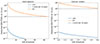Fig. 4. Detection rates of WD-fTDEs from dwarf galaxies (left panel) and from GCs (right panel) plotted for different S/N thresholds. The blue curve was calculated considering LISA as the detector, while the orange curve was obtained considering DO. The observation time for both instruments is assumed to be 10 years. The dashed black line is one event over 10 years. The occupation fraction is 1 for both scenarios.

2.5. White dwarfs: The background

The background from WD-fTDEs is expressed with the same formula as in Eq. (9), yet this time we write the rate of sources per redshift bin considering the differential rates described in Sect. 2.4. The results are illustrated in Fig. 5, where in the left panel we show WD-fTDEs background from dwarf galaxies, while in the right panel the WD-fTDEs background from GCs. As was done in the case of the MS background, we computed the S/N for these scenarios as well. In all cases, the S/N remains below 1, with the exception of the GWB produced by WD-fTDEs in dwarf galaxies. For this specific signal, the S/N for DO is approximately 19, assuming a 10-year observation period⁴.

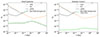Fig. 5. WD-fTDEs background from dwarf galaxies (dark green line, left panel) and WD-fTDEs background from GCs (light green line, right panel). We assume that the mass of the intermediate-mass BH in each GC is 103 M⊙ and that the occupation fraction is equal to 1 for both scenarios. Both signals are plotted with respect to the sensitivity curves of LISA (blue line), DO (orange line), and μAres (black line).

3. Repeated partial disruptions

In this section we cover rpTDEs, which occur under the empty loss cone regime, i.e., when q < 1 (cf. Section 2). We anticipate that our results show that even in an (unrealistic) optimistic scenario – with all the bursts from each TDE above threshold – the rate of detections is below one in 10 years. Nevertheless, we outline the methodology used to derive these rates, since it can also be a useful technique for other transient sources.

3.1. Individual detections

We considered four rpTDE populations, created with the methodology described in Broggi et al. (2024). In each population we have Sun-like stars, disrupted by four different BH sizes: M₁ = 10⁴ M_⊙, M₂ = 3 × 10⁵ M_⊙, M₃ = 4 × 10⁶ M_⊙, and M₄ = 10⁷ M_⊙. In each scenario, we assume that the j-th rpTDE is characterized by a constant period, P_j, between subsequent passages. This means that each rpTDE is modeled as a series of periodic bursts⁵.

Let Δt_obs represent the detector observation time, assumed to be 10 years. There are two possible scenarios:

1. long period, P_j ≥ Δt_obs: the detector observes only a single burst (the first or any subsequent one) from the j-th rpTDE, and no S/N accumulation occurs;

2. short period, P_j < Δt_obs: more consecutive bursts produced by the j-th rpTDE accumulate at the detector.

To address this, we began by considering an rpTDE characterized by an initial specific orbital energy, ϵ_j. The disruption rate for events within the energy range [ϵ_j, ϵ_j + dϵ_j] is given by

$$\begin{array}{c}\hfill {\mathrm{\Gamma }}_j=\mathrm{d}{ϵ}_j\frac{\partial \dot{N}}{\mathrm{d}{ϵ}_j}.\end{array}$$(14)

The i-th passage from the j-th rpTDE occurred at

$$\begin{array}{c}\hfill t_{\mathrm{now}}-t_{\mathrm{travel}}-(i-1)P_j,\end{array}$$(15)

where t_travel is the time the signal needs to travel from the event to the detector. This leads us to assign a weight, w, to the event (detection of the i-th burst or a sequence of bursts starting with the i-th), expressing the relative probability of observing such an event within Δt_obs.

In general, since the event has been produced between t₁ = t_now − t_travel − t₀ⁱ and t₂ = t_now − t_travel − t_fⁱ, we defined the corresponding relative weight as

$$\begin{array}{c}\hfill w\equiv \frac{{\displaystyle {\int }_{t_1}^{t_2}}{\mathrm{\Gamma }}_j\mathrm{d}t\prime }{{\displaystyle {\int }_0^{\mathrm{\Delta }{t}_{\mathrm{obs}}}}{\mathrm{\Gamma }}_j\mathrm{d}t\prime }=\frac{t_f^i-t_0^i}{\mathrm{\Delta }{t}_{\mathrm{obs}}}\end{array}$$(16)

and it can be interpreted as the fraction of relevant events.

3.2. Long period

The rate of detected rpTDEs will be

$$\begin{array}{cc}\hfill {\dot{N}}_{\det }^{\mathrm{rpTDEs}}=& {\displaystyle \int \mathrm{d}}z{\displaystyle \int \mathrm{d}}ϵ\frac{\mathrm{d}{\dot{N}}_{\det }^{\mathrm{rpTDEs}}}{\mathrm{d}z\mathrm{d}ϵ}=\hfill \\ \hfill & {\displaystyle \int \mathrm{d}}z\frac{4\pi c{\chi }^2}{H(z)}\times \frac{\mathrm{\Phi }(z)}{1+z}{\displaystyle \int \mathrm{d}}ϵ\frac{\mathrm{d}\dot{N}}{\mathrm{d}ϵ}\times \mathrm{\Theta }(ϵ,z).\hfill \end{array}$$(17)

Φ(z) is the distribution of BHs through the Universe, assuming a fixed BH mass among the four listed above. It is determined by integrating the BH mass over a specific mass bin, considering this value as a representative estimate,

$$\begin{array}{c}\hfill \mathrm{\Phi }(z)=\mathrm{\Pi }(a,b,M_{\bullet }){\displaystyle {\int }_a^b}\mathrm{d}{M}_{\bullet }\mathrm{\Phi }(M_{\bullet },z),\end{array}$$(18)

where

$$\begin{array}{c}\hfill \mathrm{\Pi }(a,b,M_{\bullet })=\mathrm{\Theta }(M_{\bullet }-a)\mathrm{\Theta }(b-M_{\bullet })=\{\begin{array}{c}1a\le M_{\bullet }\le b,\hfill \\ 0\text{else}.\hfill \end{array}\end{array}$$(19)

Each mass bin is taken centered on the BH mass considered.

The integral over the specific orbital energy can be written as a discrete sum over the energy bins,

$$\begin{array}{c}\hfill {\displaystyle {\displaystyle \sum _j}}\mathrm{\Delta }{ϵ}_j\frac{\mathrm{d}\dot{N}}{\mathrm{d}{ϵ}_j}{\mathrm{\Theta }}_j={\displaystyle \sum _j}\mathrm{\Delta }{ϵ}_j\frac{\mathrm{d}\dot{N}}{\mathrm{d}{ϵ}_j}{\displaystyle \sum _i^{N_{\mathrm{bursts}}(\mathrm{\Delta }{ϵ}_j)}}{\mathrm{\Theta }}_i.\end{array}$$(20)

Since the detector can potentially see the first or any subsequent bursts from the j-th rpTDE, the corresponding Θ_j will range from 0 to N_bursts(Δϵ_j), depending on how many bursts are above the threshold.

3.3. Short period

When the observational time is longer than the time between subsequent passages, the detector will collect signal by more passages of the same star, so that the strain of the event will accumulate. We first defined the quantities ${\stackrel{\sim }{n}}_j$ and p_j < P_j as

$$\begin{array}{c}\hfill \mathrm{\Delta }{t}_{\mathrm{obs}}={\stackrel{\sim }{n}}_j{P}_j+p_j,\end{array}$$(21)

where ${\stackrel{\sim }{n}}_j$ represents the maximum (integer) number of subsequent signals that the detector can accumulate. In particular the detector can receive

1. the first $1\le i\le {\stackrel{\sim }{n}}_j$ signals, each with weight w_α = P_j/Δt_obs;

2. a set of ${\stackrel{\sim }{n}}_j+1$ subsequent signals, each with weight w_β = p_j/Δt_obs;

3. a set of $\stackrel{\sim }{n}$ subsequent signals, each with weight w_γ = (P_j − p_j)/Δt_obs;

4. the last i signals, with $1\le i\le {\stackrel{\sim }{n}}_j$, each with weight w_δ = P_j/Δt_obs.

To better understand these categories, let us consider a practical example, where we have N_bursts = 5 and P_j = 3 years. Then we have

$$\begin{array}{c}\hfill \stackrel{\sim }{n}=3,p=1\text{year}.\end{array}$$(22)

Calling n_j = Γ_jΔt_obs the number of rpTDEs generated at energy E_j, the detector can observe the following combinations of bursts with corresponding weights:

• passage 1; total number of events: 0.3n_j;

• passage 1 and 2; total number of events: 0.3n_j;

• passage 1 and 2 and 3; total number of events: 0.3n_j;

• passage 1 and 2 and 3 and 4; total number of events: 0.1n_j;

• passage 2 and 3 and 4; total number of events: 0.2n_j;

• passage 2 and 3 and 4 and 5; total number of events: 0.1n_j;

• passage 3 and 4 and 5; total number of events: 0.3n_j;

• passage 4 and 5; total number of events: 0.3n_j;

• passage 5; total number of events: 0.3n_j.

For the detection rate, the main difference from the case described in the previous paragraph lies in the way Θ_j is expressed. Here Θ_j is the linear combination of the weighted Θ_i corresponding to the different combinations of passages. Considering the example before, Θ_j will range among 0 and

$$\begin{array}{cc}\hfill {\mathrm{\Theta }}_j=& w_{\alpha }{\mathrm{\Theta }}_1+w_{\alpha }{\mathrm{\Theta }}_2+w_{\alpha }{\mathrm{\Theta }}_3+w_{\beta }{\mathrm{\Theta }}_4+w_{\beta }{\mathrm{\Theta }}_5+w_{\gamma }{\mathrm{\Theta }}_6\hfill \\ \hfill & +w_{\delta }{\mathrm{\Theta }}_7+w_{\delta }{\mathrm{\Theta }}_8+w_{\delta }{\mathrm{\Theta }}_9=1+(N_{\mathrm{burst}}-1)\frac{P_j}{\mathrm{\Delta }{t}_{\mathrm{obs}}}\approx 2.2,\hfill \end{array}$$(23)

if all the combination of bursts are above the S/N threshold. This occurs because if the root sum square S/N of a specific combination of passages is above a certain threshold, then the corresponding Θ_i is set to 1, but it is still multiplied by a weight (less than 1). Thus, Eq. (23) states that the total Θ for the j-th rpTDE is the weighted sum of the Θ_i values for each valid burst combination of that rpTDE. The theoretical upper limit corresponds to the case in which all Θ_i are equal to 1, so the total becomes the sum of the weights for that rpTDE. Our calculation shows that none of the detector configurations under consideration will observe individual detections of these events.

3.4. The background

The background from rpTDEs is

$$\begin{array}{cc}\hfill h_{\mathrm{c},\mathrm{pop}}^2=\frac{G}{c^3{\pi }^2}\times \frac{1}{f}& {\displaystyle \sum _l}\mathrm{\Delta }{z}_l\frac{4\pi c{\chi }^2(z_l)}{H(z_l)}\times \frac{\mathrm{\Phi }(z_l)}{(1+z_{\mathrm{l}}){\chi }^2(z_l)}\hfill \\ \hfill & \times {\displaystyle \sum _j}\mathrm{\Delta }{ϵ}_j\frac{\mathrm{\Delta }\dot{N}}{\mathrm{\Delta }{ϵ}_j}{\displaystyle \sum _i^{N(\mathrm{\Delta }{ϵ}_j)}}\frac{\mathrm{d}{E}_i}{\mathrm{d}f},\hfill \end{array}$$(24)

with dE_i/df being the energy spectrum (Eq. (3)) from the i-th burst. So, contrary to the previous case for individual detections, here we sum over all passages without considering specific combinations of bursts.

The results are shown in Fig. 6, where the signals corresponding to different BH masses are represented by solid lines in various colors (M₁ = 10⁴ M_⊙ – blue, M₂ = 3 × 10⁵ M_⊙ – red, M₃ = 4 × 10⁶ M_⊙ – purple, and M₄ = 10⁷ M_⊙ – gray). The combined signal, which includes contributions from all these masses, is depicted with a dashed brown line. Notably, the most significant contribution, dominating over the others, comes from the population with M_• = 4 × 10⁶ M_⊙, which is the case in which there is the highest number of TDEs around q = 1. For higher BH masses, since all TDEs are distributed around values of q strictly smaller than one, the total GW emission is becoming less relevant. In fact, systems with a larger M_• produce TDEs exclusively in the empty loss cone regime. While this increases the number of subsequent partial disruptions, the small values of q (≲10⁻³) imply that the pericenter at which the sequence of partial disruptions occurs is so large, corresponding to lower-frequency GW bursts. This pushes the signal outside of the LISA band, as is clearly demonstrated by the corresponding contribution to the GWB shown in Fig. 6 by the gray line. The S/N for this background from rpTDEs is below 1 for all the three instruments considered.

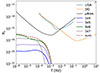Fig. 6. Background signals from different populations of rpTDEs: the solid blue line is the signal from rpTDEs with a BH of mass M• = 104 M⊙, the solid purple line the one with M• = 3 × 105 M⊙, the solid green line the one with M• = 4 × 106 M⊙, and the solid gray line the one with M• = 107 M⊙. The dashed brown line is the sum of all the backgrounds.

4. Discussion

Our study shows that the detection of rpTDEs with GWs will be unlikely in the near future. This is related to the typical values of the penetration factor that characterize these events. The penetration factor is a dimensionless quantity defined as

$$\begin{array}{c}\hfill \beta =\frac{R_{\mathrm{t}}}{R_{\mathrm{p}}},\end{array}$$(25)

which, in the empty loss cone regime, is smaller than 1. In fact, two-body relaxation is the main mechanism for a star on a given orbit to change its orbital parameters. Quantitatively, a star with a pericenter comparable to its tidal radius will stay on average 1/q periods on the same orbit before significantly changing its angular momentum (Bortolas et al. 2023). When q is small, the relaxation is very slow and stars will gradually increase their penetration factor from ∼0 up to a critical value such that in ∼1/q orbits the star is completely destroyed because of the subsequent partial disruptions happened. Since the mass lost at each passage is smaller when β is smaller, a general trend emerges: the smaller the q, the smaller the mass loss at each passage, and the smaller the corresponding penetration factor. A direct consequence is that, in a given galaxy, the greatest GW emission of repeating partial disruptions corresponds to energies such that q → 1⁻, i.e., systems with a number of repetitions on the order of unity as these stars will emit their bursts close to the tidal radius. Systems with masses of M_• ≳ 4 × 10⁶ M_⊙ produce the vast majority of their TDEs where q ≲ 10⁻², meaning that the pericenter of the corresponding rPTDEs is large. Because of the larger pericenter, empty loss cone sources result in GW emission peaked around lower frequencies than the GWs emitted by TDEs in the full loss cone scenario. In such a low-frequency window, future instruments are not sensitive enough to observe them, and also the accumulation of S/N due to multiple passages of the star around the BH is not enough to overcome this problem. As for the fTDE scenario, the situation seems more promising, as we analyze in the following.

4.1. Individual detections of fTDEs

4.1.1. MS-fTDEs: S/N

We start our analysis by examining the impact of including harmonics on the S/N of TDEs. In the left panel of Fig. 7 we plot the S/N for a MS-fTDE with a fixed BH mass of 4 × 10⁶ M_⊙ at a distance of 8 kpc. We consider stellar masses in the range 0.1 M_⊙ ≤ M_* ≤ 1 M_⊙, each disrupted at a pericenter equal to their tidal radius and, for illustrative purposes, we only consider the DO detector. The dashed line represents the S/N computed using Eq. (4), while the dots show the S/N estimates following the prescription of Pfister et al. (2022) (hereafter P22), which models the GW signal from a TDE as a monochromatic burst. The curve that includes the contribution from harmonics is consistently higher, with the discrepancy becoming more relevant at lower stellar masses, reaching up to a factor of ∼2. Additionally, we observe an interesting trend: the S/N decreases with increasing stellar mass. Although this may seem counterintuitive, it results from the signal peak shifting toward a less favorable frequency range as the stellar mass increases.

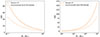Fig. 7. S/N computed for the DO instrument considered in this work. Left: S/N as a function of stellar mass for a fTDE around a 4 × 106 M⊙ BH at 8 kpc. Right: S/N as a function of BH mass for a fTDE of a 0.1 M⊙ MS star, also at 8 kpc. In both panels, the dashed line represents the S/N from Eq. (4), while the dots show the S/N estimates based on the monochromatic burst approximation (cf. Pfister et al. 2022).

In the right panel of the same figure, we consider instead the S/N of a 0.1 M_⊙ MS-star at 8 kpc, destroyed by a BH of mass ranging in the interval 10⁴ M_⊙ ≤ M_• ≤ 10⁷ M_⊙. As in the previous case, the estimate that includes all harmonic contributions yields a higher S/N, with differences reaching up to a factor of ∼2. However, in contrast to the earlier trend, the S/N ratio increases with BH mass – this is because the signal reaches a higher peak for more massive BHs.

4.1.2. MS-fTDEs: Detection rates

If we compare our results (Fig. 2) with those presented in P22 (Fig. 10)⁶, our detection rates are lower. This discrepancy is first due to the lower TDE rate adopted in this work (cf. Fig. 8 from P22 and left panel of Fig. 10 below). However, since our chosen TDE rate is based on observational constraints, we consider it a reliable estimate. Then, the detector curves that we use in this work are also different. The LISA sensitivity adopted in this study is more accurate, since we also include the noise from galactic WD binaries, which in contrast makes our curve less optimistic than the one used in P22, especially in the frequency window where the signal from MS-fTDEs peaks. For DO, the curve we use falls between the ALIA and DECIGO/BBO sensitivities presented in P22. Thus, it is not possible to do an exact one-to-one comparison. Nevertheless, our findings are consistent with the main prediction of that study, i.e., the detectors operating in the decihertz range are more likely to observe these events.

4.1.3. WD-fTDEs

As for WD-fTDEs, from Fig. 4 we conclude that we have no possible detection foreseen for LISA. However, if we consider the DO detector, the situation becomes more optimistic. Indeed, it could marginally see up to a few tens of WD-fTDEs from GCs. This is still a very uncertain number, mainly due to the strong constraints we put on our estimates (a fixed BH mass of 1000 solar masses in all the GCs and occupation fraction of 1), but given the uncertainty surrounding the presence of intermediate-mass BHs in these environments, we could not adjust these estimates any further. The detection rates instead increase to hundreds over a 10 year time observation if we consider WD-fTDEs from dwarf galaxies, with S/Ns up to ∼45. With respect to MS stars, this scenario is clearly favored due to the typical peak frequencies of these signals, ∼0.1 Hz, which fall around the most sensitive region of the detector.

4.2. The background of fTDEs

Let us now analyze the MS-background signal. As was anticipated in Sect. 2.2, a direct one-to-one comparison between our results and those of Toscani et al. (2020) (T20 from now on) is challenging due to differences in the integration limits. Therefore, our first step is to reproduce the results of T20 considering the same regime of integration, while employing our current prescription for the background. The outcome of this comparison is illustrated in Fig. 8, where we observe that, in the frequency range where the T20 signal is represented, our signal differs by approximately two orders of magnitude (before the steep fall at 0.01 Hz).

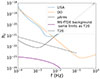Fig. 8. GWB from a population of MS-fTDEs, calculated with the same integration limits as in Toscani et al. (2020) (violet curve). The gray line represents the original signal as in Toscani et al. (2020).

To understand the origin of this discrepancy, we implemented the following modifications step by step. First of all, the limits used in T20 are the following: 0 ≤ z ≤ 3, 1 M_⊙ ≤ M_* ≤ 100 M_⊙, 10⁶ M_⊙ ≤ M_∙ ≤ 10⁸ M_⊙, and 1 ≤ β ≤ β_max(M_•, M_*). Note that in the work of T20 they consider the dimensionless parameter β instead of the pericenter, with β_max calculated assuming the pericenter equal to the Schwarzschild radius of the BH.

First, instead of using the energy spectrum described in Eq. (3), we adopted the version presented in T20. This alternative spectrum differs mainly by a constant factor of ∼80, which arises from a different approximation used in T20, as well as from the omission of harmonics. The exclusion of harmonics restores the characteristic frequency dependence f^−0.5, which is a key result highlighted in T20. Furthermore, the change in the constant factor leads to an enhancement of the signal by roughly one order of magnitude (Fig. 9, left panel).

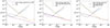Fig. 9. Steps to reproduce the signal from T20. Left panel: Use of the same energy spectrum. Central panel: In addition to the previous change, use of the same rate and BH mass function. Right panel: In addition to the previous changes, use of the same stellar mass function.

Next, employing the same TDE rate and BH mass function as in the previous work, we observe an additional increase by a factor of ∼5 (Fig. 9, central panel). Finally, we modified the stellar mass function. Instead of using the function defined in Eq. (8), normalized within the mass range (1 M_⊙, 100 M_⊙), we used the normalized stellar mass function as in T20, ∝M_*^−2.3 (Fig. 9, right panel). Thus, we recovered the results from T20.

While the difference arising from our chosen energy spectrum is inherent to the motivation of our work and cannot be altered, we illustrate in Fig. 10 the TDE rate, BH mass function, and stellar mass function used in T20 and in this study. The most significant discrepancy lies in the TDE rate, which differs by more than two orders of magnitude at both low and high BH masses. The BH mass function also shows a notable difference, particularly for BH masses above 10⁶ M_⊙. Similarly, the stellar mass function adopted in T20 assigns greater weight to more massive stars. However, our choice of TDE rate is guided by observation constraints, and the stellar mass function used in this work is more physically reasonable. We therefore regard the current, more conservative results as reliable and an updated version of the results of T20. Yet, this results in a GWB with S/N smaller than 1 even if we assume 10 years of observation for each of the three instruments.

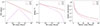Fig. 10. Left panel: TDE rate as a function of BH mass. Central panel: BH mass function (assuming a fixed redshift of z = 0.1). Right panel: Stellar mass function. In brown we show the functions used in T20, while in purple we show the functions used in this current work.

As for the WD-fTDE background, we have that the signal produced within GCs is found to be undetectable. In contrast, the GWB generated by WDs disrupted by intermediate-mass BHs in dwarf galaxies appears much more promising: with an S/N of approximately 19 over a 10-year observation period, it falls well within the sensitivity range of DO. Thus, these TDEs offer one of the most promising avenues for probing the existence of the elusive population of intermediate-mass BHs, for which observational evidence remains extremely limited to date.

5. Conclusions

In this work, we have computed the detection rates of TDEs for two future space-based GW detectors: LISA and DO. Compared to previous studies, our analysis benefits from more realistic sensitivity curves and improved modeling, including the full contribution of all harmonics in the energy spectrum.

For stars fully disrupted in a single passage, our results, although more conservative, are in agreement with previous studies and they confirm a key finding: these sources are promising targets for decihertz observatories, but unlikely to be detectable by LISA. Among the most compelling targets are WDs disrupted by intermediate-mass BHs in dwarf galaxies. These events stand out both as individually detectable sources – with detection rates over 10 years ranging from tens to hundreds depending on the S/N threshold considered – and as the only class producing a background potentially strong enough to be observed (S/N ∼ 19 over a 10-year period of observation).

Furthermore, for the first time, we have considered the GW emission from repeated disruptions, considering two scenarios: the case in which the period between each passage is longer than the detector lifetime and the case in which it is shorter, potentially leading to an accumulation of bursts (and S/N) at the detector. We find that the largest signal comes from systems with a BH mass of around 4 × 10⁶ M_⊙. Systems with less massive BHs produce only a small number of rpTDEs, and overall their GW signal decreases. Systems with larger BHs, on the other hand, predominantly produce rpTDEs, but at pericenters too large to emit detectable GW signals – even considering the accumulation of multiple passages. Unfortunately, our findings show that the detection of these events with GWs is unlikely in the near future. With this work, we provide updated estimates of the GW emission from TDEs, and we hope that this can be a useful reference to drive the development of decihertz detectors.

Acknowledgments

MT, LB and AS acknowledge financial support provided under the European Union’s H2020 ERC Consolidator Grant “Binary Massive Black Hole Astrophysics” (B Massive, Grant Agreement: 818691). MT acknowledges N. Tamanini for useful feedback. MT acknowledges N. Cuello for continuous support.

References

Appendix A: Occupation fraction

While calculating the WD-fTDEs detection rates and background for dwarf galaxies, we considered the same BH mass function as in Pfister et al. 2022, which assumes an occupation fraction of 1. While this is in general true for supermassive BHs in galactic cores, the situation for intermediate-mass BHs is likely different and dependent on the galaxy mass. To account for this, we repeated the calculation using an occupation fraction that depends on the stellar mass of the host galaxy. This factor enters Eq. (6) as a multiplicative term modifying the BH mass function. Specifically, we implemented the parametrization proposed by Gallo & Sesana 2019,

$$\begin{array}{c}\hfill {\lambda }_{\mathrm{occ}}(M_{\mathrm{gal}})=0.5+0.5\ast tanh(2.5^{|8.9-log{M}_{\mathrm{gal},0}/M_{\odot }|}log\frac{M_{\mathrm{gal}}}{M_{\mathrm{gal},0}}),\end{array}$$(A.1)

with M_gal galaxy stellar mass and M_gal, 0 parameter that we assume equal to 10^8.17 M_⊙ (cf. Fig. 1 of Gallo & Sesana 2019). M_gal can be converted in the BH mass using the relation from Reines & Volonteri 2015. The results obtained using this revised occupation fraction are shown in Fig. A.1. The left panel presents the individual detection rates, while the right panel displays the background. Although some variations are noticeable, they do not significantly impact the conclusions discussed in the main body of the paper. Given this, and considering the current uncertainties surrounding the distribution of intermediate-mass BHs in dwarf galaxies, we regard the results in the main text as a valid upper limit. For GCs, the situation is even more uncertain. To explore the impact on detection rates, we simply assume a constant occupation fraction λ_occ. This parameter acts as a multiplicative factor on the TDE rate per cluster, while the GWB scales with $\sqrt{{\lambda }_{\mathrm{occ}}}$. Also in this scenario, given the significant uncertainty associated with this parameter, we continue to treat the results presented in the main text as a valid upper limit.

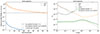Fig. A.1. Left panel: detection rates of WD-fTDEs from dwarf galaxies plotted for different S/N thresholds. Right panel: GWB from WD-fTDEs from dwarf galaxies. The color scheme and the detectors are the same as in Fig. 4-5. The solid line represents an occupation fraction of 1, while the dotted line an occupation fraction as in Gallo & Sesana 2019.

Appendix B: Lighter intermediate-mass BH

We have also investigated the GW signal from a population of WD–fTDEs occurring in GCs hosting BHs with masses of 500M_⊙. As shown in Fig. B.1, both the detection rates and the background are generally lower than those presented earlier in the main text, making the detection of such events even less likely. However, obtaining a more realistic estimate will ultimately require observational constraints on the intermediate-mass BH population in GCs.

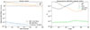Fig. B.1. Left panel: detection rates of WD-fTDEs from GCs plotted for different S/N thresholds. Right panel: GWB from WD-fTDEs from GCs. The color scheme and the detectors are the same as in Fig. 4-5. The solid line represents an intermediate-mass BH of 103M⊙, while the dotted line one of 500M⊙.

All Figures

	Fig. 1. GW signal from a fTDE of a 0.1 M⊙ MS star disrupted by a 4 × 106 M⊙ BH (gray lines) and GW signal from a fTDE of a WD of 0.5 M⊙ disrupted by a 103 M⊙ BH (red lines). We consider two possible source distances: 8 kpc (dashed lines) and 1 Mpc (dash-dotted lines). In blue and orange, we plot the noise amplitudes of LISA and DO, respectively.
In the text

	Fig. 2. Detection rates of MS-fTDEs plotted for different S/N thresholds. The blue curve was calculated considering LISA as the detector, while the orange curve was obtained considering DO. The observation time for both instruments is assumed to be 10 years. The dashed black line is one event over 10 years.
In the text

	Fig. 3. MS-fTDEs background (magenta curve) plotted with respect to the sensitivity curves of LISA (blue line), DO (orange line), and μAres (black line).
In the text

Fig. 4. Detection rates of WD-fTDEs from dwarf galaxies (left panel) and from GCs (right panel) plotted for different S/N thresholds. The blue curve was calculated considering LISA as the detector, while the orange curve was obtained considering DO. The observation time for both instruments is assumed to be 10 years. The dashed black line is one event over 10 years. The occupation fraction is 1 for both scenarios.

In the text

Fig. 5. WD-fTDEs background from dwarf galaxies (dark green line, left panel) and WD-fTDEs background from GCs (light green line, right panel). We assume that the mass of the intermediate-mass BH in each GC is 103 M⊙ and that the occupation fraction is equal to 1 for both scenarios. Both signals are plotted with respect to the sensitivity curves of LISA (blue line), DO (orange line), and μAres (black line).

In the text

	Fig. 6. Background signals from different populations of rpTDEs: the solid blue line is the signal from rpTDEs with a BH of mass M• = 104 M⊙, the solid purple line the one with M• = 3 × 105 M⊙, the solid green line the one with M• = 4 × 106 M⊙, and the solid gray line the one with M• = 107 M⊙. The dashed brown line is the sum of all the backgrounds.
In the text

Fig. 7. S/N computed for the DO instrument considered in this work. Left: S/N as a function of stellar mass for a fTDE around a 4 × 106 M⊙ BH at 8 kpc. Right: S/N as a function of BH mass for a fTDE of a 0.1 M⊙ MS star, also at 8 kpc. In both panels, the dashed line represents the S/N from Eq. (4), while the dots show the S/N estimates based on the monochromatic burst approximation (cf. Pfister et al. 2022).

In the text

	Fig. 8. GWB from a population of MS-fTDEs, calculated with the same integration limits as in Toscani et al. (2020) (violet curve). The gray line represents the original signal as in Toscani et al. (2020).
In the text

	Fig. 9. Steps to reproduce the signal from T20. Left panel: Use of the same energy spectrum. Central panel: In addition to the previous change, use of the same rate and BH mass function. Right panel: In addition to the previous changes, use of the same stellar mass function.
In the text

	Fig. 10. Left panel: TDE rate as a function of BH mass. Central panel: BH mass function (assuming a fixed redshift of z = 0.1). Right panel: Stellar mass function. In brown we show the functions used in T20, while in purple we show the functions used in this current work.
In the text

	Fig. A.1. Left panel: detection rates of WD-fTDEs from dwarf galaxies plotted for different S/N thresholds. Right panel: GWB from WD-fTDEs from dwarf galaxies. The color scheme and the detectors are the same as in Fig. 4-5. The solid line represents an occupation fraction of 1, while the dotted line an occupation fraction as in Gallo & Sesana 2019.
In the text

	Fig. B.1. Left panel: detection rates of WD-fTDEs from GCs plotted for different S/N thresholds. Right panel: GWB from WD-fTDEs from GCs. The color scheme and the detectors are the same as in Fig. 4-5. The solid line represents an intermediate-mass BH of 103M⊙, while the dotted line one of 500M⊙.
In the text

References

- Arca Sedda, M., Berry, C. P. L., Jani, K., et al. 2020, Class. Quantum Gravity, 37, 215011 [Google Scholar]
- Berry, C. P. L., & Gair, J. R. 2010, Phys. Rev. D, 82, 107501 [Google Scholar]
- Bortolas, E., Ryu, T., Broggi, L., & Sesana, A. 2023, MNRAS, 524, 3026 [NASA ADS] [CrossRef] [Google Scholar]
- Broggi, L., Stone, N. C., Ryu, T., et al. 2024, Open J. Astrophys., 7, 48 [CrossRef] [Google Scholar]
- Chang, J. N. Y., Dai, L., Pfister, H., & Chowdhury, R. K. 2025, ApJ, 980, L22 [Google Scholar]
- Colpi, M., Danzmann, K., Hewitson, M., et al. 2024, ArXiv e-prints [arXiv:2402.07571] [Google Scholar]
- Davidzon, I., Ilbert, O., Laigle, C., et al. 2017, A&A, 605, A70 [NASA ADS] [CrossRef] [EDP Sciences] [Google Scholar]
- Franchini, A., Bonetti, M., Lupi, A., et al. 2023, A&A, 675, A100 [NASA ADS] [CrossRef] [EDP Sciences] [Google Scholar]
- Frank, J., & Rees, M. J. 1976, MNRAS, 176, 633 [NASA ADS] [CrossRef] [Google Scholar]
- Gallo, E., & Sesana, A. 2019, ApJ, 883, L18 [NASA ADS] [CrossRef] [Google Scholar]
- Gomez, S., Villar, V. A., Berger, E., et al. 2023, ApJ, 949, 113 [Google Scholar]
- Harris, G. L. H., & Harris, W. E. 2011, MNRAS, 410, 2347 [NASA ADS] [CrossRef] [Google Scholar]
- Hogg, D. W. 1999, ArXiv e-prints [arXiv:astro-ph/9905116] [Google Scholar]
- Ivezić, Ž., Kahn, S. M., Tyson, J. A., et al. 2019, ApJ, 873, 111 [Google Scholar]
- Kobayashi, S., Laguna, P., Phinney, E. S., & Mészáros, P. 2004, ApJ, 615, 855 [Google Scholar]
- Kroupa, P. 2001, MNRAS, 322, 231 [NASA ADS] [CrossRef] [Google Scholar]
- Linial, I., & Metzger, B. D. 2023, ApJ, 957, 34 [NASA ADS] [CrossRef] [Google Scholar]
- Maggiore, M. 2008, in Gravitational Waves: Volume 1: Theory and Experiments, Gravitational Waves (OUP Oxford) [Google Scholar]
- Pfister, H., Toscani, M., Wong, T. H. T., et al. 2022, MNRAS, 510, 2025 [Google Scholar]
- Phinney, E. S. 1989, IAU Symp., 136, 543 [Google Scholar]
- Phinney, E. S. 2001, ArXiv e-prints [arXiv:astro-ph/0108028] [Google Scholar]
- Rees, M. J. 1988, Nature, 333, 523 [Google Scholar]
- Reines, A. E., & Volonteri, M. 2015, ApJ, 813, 82 [NASA ADS] [CrossRef] [Google Scholar]
- Rossi, E. M., Stone, N. C., Law-Smith, J. A. P., et al. 2021, Space Sci. Rev., 217, 40 [NASA ADS] [CrossRef] [Google Scholar]
- Saxton, R., Komossa, S., Auchettl, K., & Jonker, P. G. 2021, Space Sci. Rev., 217, 18 [NASA ADS] [CrossRef] [Google Scholar]
- Sesana, A. 2016, Phys. Rev. Lett., 116, 231102 [NASA ADS] [CrossRef] [Google Scholar]
- Sesana, A., Korsakova, N., Arca Sedda, M., et al. 2021, Exp. Astron., 51, 1333 [NASA ADS] [CrossRef] [Google Scholar]
- Shvartzvald, Y., Waxman, E., Gal-Yam, A., et al. 2024, ApJ, 964, 74 [NASA ADS] [CrossRef] [Google Scholar]
- Stone, N. C., & Metzger, B. D. 2016, MNRAS, 455, 859 [NASA ADS] [CrossRef] [Google Scholar]
- Stone, N. C., Vasiliev, E., Kesden, M., et al. 2020, Space Sci. Rev., 216, 35 [NASA ADS] [CrossRef] [Google Scholar]
- Toscani, M., Rossi, E. M., & Lodato, G. 2020, MNRAS, 498, 507 [Google Scholar]
- Toscani, M., Lodato, G., Price, D. J., & Liptai, D. 2022, MNRAS, 510, 992 [Google Scholar]
- Toscani, M., Rossi, E. M., Tamanini, N., & Cusin, G. 2023, MNRAS, 523, 3863 [Google Scholar]
- van Velzen, S., Holoien, T. W. S., Onori, F., Hung, T., & Arcavi, I. 2020, Space Sci. Rev., 216, 124 [CrossRef] [Google Scholar]