| Issue |
A&A
Volume 703, November 2025
|
|
|---|---|---|
| Article Number | A223 | |
| Number of page(s) | 11 | |
| Section | Extragalactic astronomy | |
| DOI | https://doi.org/10.1051/0004-6361/202555721 | |
| Published online | 26 November 2025 | |
The baryonic mass–size relation of galaxies
I. A dichotomy in star-forming galaxy disks
1
Arcetri Astrophysical Observatory, INAF, Largo Enrico Fermi 5, 50125 Florence, Italy
2
Department of Astronomy, University of Science and Technology of China, Hefei 230026, China
3
School of Astronomy and Space Sciences, University of Science and Technology of China, Hefei 230026, China
4
Dipartimento di Fisica e Astronomia, Università degli Studi di Firenze, 50019 Sesto Fiorentino, Italy
5
Department of Astronomy, Case Western Reserve University, 10900 Euclid Avenue, Cleveland, OH 44106, USA
6
Department of Physics, University of Oregon, Eugene, OR 97403, USA
⋆ Corresponding author: This email address is being protected from spambots. You need JavaScript enabled to view it.
Received:
29
May
2025
Accepted:
1
October
2025
Abstract
The mass–size relations of galaxies are generally studied considering only stars or only gas separately. Here we study the baryonic mass–size relation of galaxies from the SPARC database, using the total baryonic mass (Mbar) and the baryonic half-mass radius (R50, bar). We find that SPARC galaxies define two distinct sequences in the Mbar − R50, bar plane: one that formed by high-surface-density (HSD), star-dominated, Sa-to-Sc galaxies, and one by low-surface-density (LSD), gas-dominated, Sd-to-dI galaxies. The Mbar − R50, bar relation of LSD galaxies has a slope close to 2, pointing to a constant average surface density, whereas that of HSD galaxies has a slope close to 1, indicating that less massive spirals are progressively more compact. Our results point to the existence of two types of star-forming galaxies that follow different evolutionary paths: HSD disks are very efficient in converting gas into stars, perhaps thanks to the efficient formation of non-axisymmetric structures (bars and spiral arms), whereas LSD disks are not. The HSD-LSD dichotomy is absent in the baryonic Tully-Fisher relation (Mbar versus flat circular velocity Vf) but moderately seen in the angular–momentum relation (approximately Mbar versus Vf × R50, bar), so it is driven by variations in R50, bar at fixed Mbar. This fact suggests that the baryonic mass–size relation is the most effective empirical tool to distinguish different galaxy types and study their evolution.
Key words: galaxies: dwarf / galaxies: evolution / galaxies: kinematics and dynamics / galaxies: spiral / galaxies: structure
© The Authors 2025
 Open Access article, published by EDP Sciences, under the terms of the Creative Commons Attribution License (https://creativecommons.org/licenses/by/4.0), which permits unrestricted use, distribution, and reproduction in any medium, provided the original work is properly cited.
This article is published in open access under the Subscribe to Open model. This email address is being protected from spambots. You need JavaScript enabled to view it. to support open access publication.
1. Introduction
One of the best studied scaling relations of galaxies is the stellar mass–size relation (e.g. Gadotti 2009; Lange et al. 2015), which relates the stellar mass (M⋆) to the effective radius (R50, ⋆). The effective radius is generally defined as the radius that encompasses half of the stellar light or stellar mass of a galaxy, so it is also referred to as half-light or half-mass radii. Strictly speaking, the effective radius is not a measurement of ‘size’ with the usual intuitive meaning of ‘maximum spatial extension’ of an object because galaxies do not have a hard boundary. Rather, the half-mass radius is a measurement of how concentrated the stellar mass or stellar light is (de Vaucouleurs 1948). Other possible definitions of ‘galaxy sizes’ consider isophotal or isodensity radii, which are taken at some fixed surface brightness (e.g. the Holmberg radius) or surface density value (e.g. Trujillo et al. 2020). For the sake of simplicity, hereafter we use the terms ‘effective radius’, ‘half-mass radius’, and ‘size’ in an interchangeable way.
The stellar mass–size relation has been studied in connection with other galaxy properties, such as their morphology (e.g. Shen et al. 2003; Bernardi et al. 2014; Schombert 2006), surface brightness (e.g. Greene et al. 2022), specific star formation rates (e.g. Nedkova et al. 2024), specific angular momentum (e.g. Kim & Lee 2013; Rong et al. 2017), interactions and mergers (e.g. Du et al. 2024b; Liao et al. 2019), and environment (e.g. Fernández Lorenzo et al. 2013; Rodriguez et al. 2021; Afanasiev et al. 2023). In addition, one can probe the assembly history of galaxies by observing the evolution of the stellar mass–size relation with redshift (e.g. van der Wel et al. 2014; Roy et al. 2018; Mowla et al. 2019; Yang et al. 2021; Afanasiev et al. 2023; Nedkova et al. 2024). One can also study the distinct mass–size relations of different stellar components in galaxies, such as bulges and disks, in order to trace their evolutionary paths separately (e.g. Nedkova et al. 2024). The stellar mass–size relation has also been extensively investigated in the Λ cold dark matter (ΛCDM) paradigm of galaxy formation, in particular in relation to the halo spin (Mo et al. 1998; Dutton et al. 2007; Kim & Lee 2013; Rong et al. 2017; Liao et al. 2019) and/or halo virial radius (Kravtsov 2013; Huang et al. 2017; Somerville et al. 2018; Rodriguez et al. 2021).
Another well-studied structural relation is the H I mass–size relation of star-forming galaxies (Broeils & Rhee 1997). Given that atomic hydrogen largely dominates the gas budget of star-forming galaxies (e.g. Cortese et al. 2017), the H I mass–size relation is effectively the gaseous counterpart of the stellar mass–size relation. For historical reasons, the H I radius (RHI) is not defined as the radius that contains 50% of the H I mass, but rather as the radius where the H I surface density equals 1 M⊙ pc−2 (after correction to face-on view), so it is effectively an isophotal radius. Interestingly, the H I mass–size relation has a slope close to 2, indicating that the average surface densities of H I disks are approximately constant (Broeils & Rhee 1997; Verheijen & Sancisi 2001; Swaters et al. 2002; Lelli et al. 2016a; Wang et al. 2016; Lutz et al. 2018; Gault et al. 2021). This phenomenon may be related to the transformation of H I into H2 (Stevens et al. 2019), which is a crucial step in the star formation process.
Previous studies of the mass–size relation of galaxies focussed either only on stars or only on gas, but galaxies consist of both mass components. In particular, in star-forming dwarf galaxies, the gas mass can be comparable or even higher than the stellar mass (e.g. Lelli 2022), so neither the stellar mass–size relation nor the gaseous mass–size relation can thoroughly trace the matter distribution in their disks. In this paper, we study the baryonic mass–size relation of star-forming galaxies, linking the total baryonic mass (Mbar = M⋆ + Mgas) with the baryonic effective radius (R50, bar) that encloses half of Mbar.
The rest of this paper is structured as follows. In Section 2, we describe our sample and the derivation of Mbar and R50, bar. In Section 3, we present our results and find that star-forming galaxies follow two distinct sequences: one defined by high-surface-density (HSD) galaxies and one by low-surface-density (LSD) ones. In Section 4, we discuss the HSD-LSD dichotomy in relation to the previous literature as well as to other galaxy scaling laws, such as the baryonic Tully–Fisher relation (BTFR) and the angular momentum relation (AMR). Finally, in Section 5, we provide a brief summary of our results.
2. Data analysis
2.1. Gas and stellar surface density profiles
The half-mass radius can be measured either by fitting a parametric function (such as the Sérsic 1963 profile) to the matter distribution, or by constructing the so-called ‘curve of growth’ (CoG) that gives the cumulative mass as a function of radius R. In general, the baryonic mass distribution of galaxies cannot be described by a simple parametric function, so we computed R50, bar by constructing the baryonic CoG (Fig. 1). This requires the gas and stellar surface density profiles corrected for face-on view.
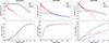 |
Fig. 1. Measurements of R50, gas, R50, ⋆, and R50, bar for three example galaxies: a gas-dominated one (UGC 731), a star-dominated one (NGC 2903), and an intermediate case (NGC 5585). The upper panels show the surface density profiles for gas (blue points), stars (red points), and total baryons (black line); the stellar profile was extrapolated at large radii with an exponential function (dashed red line). The lower panel shows the curve of growth of gas (blue line), stars (red line), and total baryons (black line); the dotted lines show the location of the corresponding half-mass radii. |
The Surface Photometry and Accurate Rotation Curves (SPARC) sample is the ideal dataset for our purposes because it contains 175 disk galaxies (Sa to dI)1 with both near-infrared (NIR) images at 3.6 μm from Spitzer, tracing the stellar mass distribution, and interferometric H I data, tracing the gas distribution and kinematics (Lelli et al. 2016a). The first SPARC data release (Lelli et al. 2016a), however, did not provide the H I surface density profiles because the gravitational contribution of the gas disk (parametrized via the expected circular velocity Vgas) was directly taken from previous works. Thus, we searched the literature and found H I surface density profiles for 169 galaxies out of 175 galaxies. Unfortunately, for the remaining six galaxies (D512-2, D564-8, D631-7, NGC 5907, NGC 4138, UGC 06818), the H I rotation-curve references do not provide the H I surface density profiles. The references for the H I surface density profiles are listed in Table A.1. In general, these authors use a consistent method to derive the H I surface density profiles, that is taking azimuthal averages over a fixed set of rings, whose geometry (centre, position angle, and inclination angle i) is set by the H I kinematics (e.g. Begeman 1987). An exception is represented by edge-on galaxies (with i ≳ 80°) for which the H I surface density profiles are derived using the Lucy deconvolution method (see Swaters et al. 2002, for details). Our sample contains only 24 edge-on galaxies; they do not show any sign of systematic effect with respect to the rest of the sample.
To obtain the face-on H I surface density profiles, we followed the same procedure applied by Lelli et al. (2016a) to the NIR surface brightness profiles. In short, we ran the task Rotmod in the GIPSY software (Vogelaar et al. 2001), which takes the observed surface brightness profile and total disk mass as inputs, then returns the expected circular velocity and face-on surface density as outputs. We used the same H I masses and distances given in Lelli et al. (2016a). In running Rotmod, we assumed an exponential vertical density profile with scale height of 100 pc (as in Lelli et al. 2016a), but this assumption plays virtually no role because we are interested in the face-on surface density integrated along the z axis of the disk.
The H I and NIR data have different spatial resolutions, so the resulting surface brightness profiles are sampled at different radii. To sum up the two components, the profiles were linearly interpolated and sampled on a common radial grid. Different choices in the interpolation play virtually no role in the final measurement of the half-mass radii. During this analysis, we also revisited some bulge-disk decompositions and outer extrapolations of the stellar profiles to ensure that the resulting CoGs are well-behaved with no unphysical jumps or discontinuities. We recall that SPARC bulge-disk decompositions are non-parametric and assign non-axisymmetric structures (bars, lenses, pseudo-bulges) to the stellar disk (Lelli et al. 2016a). As we show in Sect. 3.3, including or excluding bulges gives no differences at all in the baryonic mass–size relation of LSD galaxies (mostly Sd-to-dI types) and only small differences in the one of HSD galaxies (mostly Sa-to-Sc types), so it is clear that bulge-disk decompositions represent a second-order detail, at least for what concerns the SPARC sample.
2.2. Gas and stellar masses
The final step to build the baryonic CoG is to choose appropriate mass-to-light ratios for the stellar disk (Υ⋆,disk) and the stellar bulge (Υ⋆,bul), as well as the factor to correct the H I mass for the contribution of heavier elements (Mgas/MH I). In analogy to previous SPARC papers, we assumed Υ⋆,disk = 0.5, Υ⋆,bul = 0.7, and Mgas/MH I = 1.33 for all galaxies. The choice of constant values provides the most empirical and data-driven representation of the data because it merely puts gas mass and stellar mass on a common physical scale, without any model-dependent variation from galaxy to galaxy (or within a given galaxy). Variations in Υ⋆ were taken into account in our error budget, which considered uncertainties of 25% due to plausible differences in the galaxy star formation history and chemical enrichment history (e.g. Schombert et al. 2019, 2022).
It is possible to choose variable mass-to-light ratios (e.g. Schombert et al. 2022; Duey et al. 2025) and/or gas correction factors (McGaugh et al. 2020) from galaxy to galaxy; we will investigate such potential improvements in future work. As a preliminary study, we considered the values of Υ⋆ from fitting the spectral energy distribution (SED) of 110 SPARC galaxies (Marasco et al. 2025). We find that Υ⋆ from SED fitting have negligible effects on our final results because they deviate from our fiducial values only in gas-dominated dwarf galaxies (see Fig. 1 of Marasco et al. 2025), in which the stellar component plays little role in the values of Mbar and R50, bar. This is in line with the fact that the scatter in the (stellar or baryonic) Tully–Fisher relation does not decrease using Υ⋆ from SED fitting, but rather increases with respect to the simple choice of a constant Υ⋆ at 3.6 μm (Ponomareva et al. 2018; Marasco et al. 2025).
Formally, our measurements of Mbar and R50, bar neglect molecular gas. On average, the molecular gas mass (Mmol) of nearby galaxies is about 7% of the stellar mass (McGaugh et al. 2020; Saintonge & Catinella 2022), so its contribution to Mbar is generally small (but the scatter in the Mmol/M⋆ ratio can be significant, see Calette et al. 2018). Broadly speaking, molecular gas has a similar spatial distribution as the stellar disk on large (kpc) scales (Leroy et al. 2008; Frank et al. 2016), so its contribution could be implicitly included in the stellar density profile. On average, this would be equivalent to assuming Υ⋆,disk = 0.535 rather than Υ⋆,disk = 0.5. This small statistical correction would make no difference to our results because it is smaller than expected variations in Υ⋆, which are ultimately the most relevant uncertainties in the measurements of Mbar and R50, bar.
Fig. 1 shows the baryonic CoG for three characteristic galaxies: a gas-dominated case, a star-dominated case, and an intermediate case. For the gas-dominated galaxy, the baryonic half-mass radius is nearly identical to the gaseous half-mass radius (R50, gas). Conversely, for the star-dominated galaxy, one has R50, bar ≃ R50, ⋆. For the intermediate case, R50, bar is somewhat in between R50, gas and R50, ⋆, highlighting the importance of considering both stars and gas when studying galaxy sizes. Notably, when the gas contribution is substantial, the baryonic CoG may not show a clear flattening as in the case of the stellar CoG because gas disks are generally more diffuse than stellar disks (see Fig. 1). The H I data used here reach H I column densities of about 5 − 10 × 1019 cm−2 (the typical H I sensitivity of historic radio interferometers), so they may not trace the full extent of the H I disks. Recent, ultra-deep H I observations with the MeerKAT telescope (the MHONGOOSE survey; de Blok et al. 2024; Marasco et al. 2025) show that the sizes of H I disks do not increase substantially when probing column densities that are 2 orders of magnitude lower (a few times 1017 cm−2, see Fig. 7 in de Blok et al. 2024), so some of our Mbar and R50, bar may be underestimated by 10%−20% at most, which is comparable to or smaller than our assumed uncertainties (see Appendix B).
3. Results
3.1. Two sequences in the baryonic mass–size plane
Figure 2 shows the gaseous, stellar, and baryonic mass–size relations of SPARC galaxies, colour-coded by their gas fraction fgas = Mgas/Mbar. The gaseous mass–size relation (left panel) is a tight power law (in logarithmic space), in agreement with previous studies that used the ‘isophotal’ H I radius (e.g. Broeils & Rhee 1997; Verheijen & Sancisi 2001; Swaters et al. 2002; Lelli et al. 2016a; Wang et al. 2016). The stellar mass–size relation (middle panel) displays two distinct sequences, which were noted by Lelli et al. (2016a) in the luminosity-size plane (their Fig. 2) and are in agreement with the seminal work of Schombert (2006). These two sequences approximately correspond to high surface brightness (HSB), star-dominated, early-type spirals (Sa to Sc) and to low surface brightness (LSB), gas-dominated, late-type disks (Sd to dI). The baryonic mass–size relation (right panel) makes the two sequences even more evident. The LSB sequence, indeed, becomes tighter because it mostly consists of gas-dominated objects, highlighting the importance of adding the gas component in the mass–size relation. If we use the radius that encompasses 20% or 80% of the baryonic mass (R20, bar and R80, bar) instead of R50, bar, two distinct HSB-LSB sequences persist, indicating that their existence does not depend on the specific definition of the baryonic radius. In the following, we consider baryonic surface densities rather than surface brightnesses, so we refer to the two distinct populations as high-surface-density (HSD) and low-surface-density (LSD) galaxies.
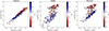 |
Fig. 2. Gaseous (left panel), stellar (middle panel), and baryonic (right panel) mass–size relations of SPARC galaxies. Data points are colour-coded by the gas fraction fgas; the error bars denote the 1σ errors. The three panels span the same dynamic range on both axes. Two sequences are evident in the stellar and baryonic mass–size relations. |
The existence of two distinct sequences is confirmed by the DBSCAN algorithm (Ester et al. 1996), which can be used to identify clusters of points. This algorithm is robust against irregular boundaries and does not need a priori information about the number of clusters. We adopted the DBSCAN package in SCIKIT-LEARN (Pedregosa et al. 2011), and used it in a normalized five-dimensional space, consisting of log(Mbar), log(R50, bar), gas fraction fgas, Hubble type T, and effective surface density log(Σ50, bar). The gas fraction is defined as fgas = Mgas/Mbar, while the baryonic effective surface density as Σ50, bar = Mbar/(2πR50, bar2). Following Ester et al. (1996), we determined the best input parameters of DBSCAN as Eps = 0.239 and Min_samples = 10. These two parameters work as follows: For a given data point in the parameter space, any other point within a radius equal to Eps is considered as its neighbour. If the number of neighbours of a given point is greater than Minpts, the point will be considered as a ‘core point’, so as the core of a cluster of points.
As expected, DBSCAN divides our sample of galaxies into two main groups (plus a few outliers). Figure 3 shows that the two groups separate around fgas ≃ 0.3, T ≃ 5 (corresponding to Sc types), and log(Σ50, bar/[M⊙ pc−2])≃2.1. This clustering result is robust for a broad range of input parameters, specifically Eps ∈[0.18, 0.25] and Minpts ∈[7, 13]. We then used the characteristic value Σc ≃ 125 M⊙ pc−2 to divide our sample into LSD (Σ50, bar < Σc) and HSD (Σ50, bar ≥ Σc) galaxies. Using a characteristic fgas or T instead of Σc provides similar results in terms of separating two galaxy populations. Of course, any separation is a simplification because there is no sharp transition in galaxy properties: there are galaxies in-between the two sequences that are mostly Sc/Sd types with intermediate surface brightness and fgas ≃ 0.3 − 0.5.
 |
Fig. 3. Distributions of fgas, Σ50, bar, T, and μ0, disk for the two groups identified by DBSCAN (red and blue histograms). The dashed black lines show the separation values reported in Table A.2. Panels (a)–(c) show the distributions clustered by logΣ50, bar, while panel (d) shows the distributions clustered by μ0, disk (after correction to a face-on view). |
3.2. Best-fit baryonic mass–size relations
We fitted each galaxy group with a straight line,
 (1)
(1)
where α is the slope, β is the intercept. Fitting a straight line to data points with intrinsic scatter and errors on both variables is not a trivial exercise. For example, the BAYESLINEFIT software (Lelli et al. 2019) uses a Markov-chain Monte-Carlo approach in a Bayesian framework, assuming that the two variables are independent. In the case of the mass–size relation, however, the two variables are not independent because they both vary with galaxy distance D (Mbar ∝ D2 and R50, bar ∝ D). Thus, we used the ROXY package (Bartlett & Desmond 2023) that can take the covariance between the variables into account. Details on the estimation of the covariance matrix are given in Appendix B. The current implementation of ROXY, however, can fit only for the vertical intrinsic scatter, not the orthogonal intrinsic scatter perpendicular to the best-fit line. Appendix A of Lelli et al. (2019) discusses the systematic differences between the two approaches (see also Appendix C).
The best-fit relations are shown in Fig. 4 (left panel), and the best-fit parameters are shown in Table A.2. The baryonic mass–size relation of LSD galaxies has α = 1.95 ± 0.12, while that of HSD galaxies has α = 1.08 ± 0.18. The former value implies that LSD galaxies share a similar Σ50, bar ≃ 13 M⊙ pc−2, which is largely driven by the gas component. On the other hand, HSD galaxies become less dense and compact as their Mbar increase. Interestingly, the intrinsic scatter (σint) of the HSD sequence (σint = 0.30 ± 0.03) and the LSD sequence (σint = 0.32 ± 0.02) are consistent within the errors. The HSD sequence shows higher observed scatter (evident by eye) because Mbar is dominated by the stellar mass, which has higher uncertainties than the gas mass dominating Mbar in the LSD sequence. Intrinsically, however, the two sequences may be similarly tight.
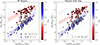 |
Fig. 4. Baryonic mass–size relations considering all baryons (left panel) and the baryonic disks only (excluding stellar bulges, right panel). Galaxies are colour-coded by the gas fraction fgas. Crosses represent S0-to-Sc galaxies (Hubble type T ≤ 5), while circles represent Sd-to-dI galaxies (T > 5). The red and the blue solid lines show the best-fit relations to the HSD and LSD sequences, respectively; the red and blue shaded areas indicate the best-fit intrinsic scatters. Dashed lines correspond to constant surface densities for multiples of Σc = 125 M⊙ pc−2 (see Sect. 3 for details). |
3.3. The effect of stellar bulges
One may wonder whether the HSD-LSD dichotomy is driven by the presence of stellar bulges because HSD galaxies mostly have early Hubble types (Sa-Sc), whereas LSD galaxies are virtually bulgeless (Sd-dI). Indeed, Lelli et al. (2016a) performed bulge-disk decompositions for only two peculiar LSD galaxies out of 118, whereas bulge-disk decompositions were performed for 28 HSD galaxies out of 51 (mostly Sa-Sb types). We used these bulge-disk decompositions to measure the baryonic CoG of the baryonic disk (stars plus gas) and its half-mass radius, R50, disk, excluding the bulge component. Importantly, the non-parametric bulge-disk decompositions of Lelli et al. (2016a) assign stellar bars, ovals, and small pseudo-bulges to the disk component. These structures are mostly present in HSD galaxies and are known to arise from the disk secular evolution, so they probably share a similar Υ⋆ as the rest of the disk.
Fig. 4 (right panel) shows the baryonic-disk mass–size relation, excluding stellar bulges. The two HSD-LSD sequences are still evident by eye, and formally confirmed by the DBSCAN algorithm. Thus, the HSD-LSD dichotomy is not driven by the presence of stellar bulges. For LSD galaxies, the best-fit Mdisk − R50, disk relation is virtually the same as the Mbar − R50, bar relation, as expected given the lack of stellar bulges. For HSD galaxies, instead, the best-fit Mdisk − R50, disk relation has a slightly steeper slope (α = 1.36 ± 0.16) than the Mbar − R50, bar relation (α = 1.08 ± 0.18), but the two slopes are consistent within 1.16σ (see also Appendix A). This fact indicates that the details of the bulge-disk decompositions do not play an important role in our general results. Finally, we note that Sc/Sd galaxies (with small or no bulges) mostly fill the gap between the two sequences, suggesting that the onset of bulges could depend on the mean surface density of the baryonic disk. In other words, the existence of bulges in HSD disks may be a direct effect of the dichotomy, as we discuss in Sect. 4.1.
4. Discussion
4.1. A dichotomy in star-forming galaxy disks
The existence of two sequences in the Mbar − R50, bar plane suggests that there is a dichotomy in star-forming disks: galaxies tend to be either HSD or LSD, so tend to avoid intermediate surface densities around 100 M⊙ pc−2. It is then natural to ask whether the observed HSD-LSD dichotomy may be driven by potential selection effects. The SPARC sample is the result of decades of interferometric H I observations from different groups (see Lelli et al. 2016a, for references), so it does not have a well-defined selection function. However, selection effects should generally bias against LSD or LSB galaxies, which are instead very well represented in SPARC. We cannot identify any sensible observational effect that would bias against intermediate surface densities. The upcoming BIG-SPARC database (Haubner et al. 2024), which will combine H I observations with NIR photometry for thousands of galaxies, will clarify the situation.
Reassuringly, the same dichotomy was found by Schombert (2006) studying the stellar mass–size plane of a different galaxy sample. In addition, a similar dichotomy was found in terms of the disk central surface brightness μ0, disk in other independent studies (Tully & Verheijen 1997; McDonald et al. 2009a,b; Sorce et al. 2013, 2016). Clearly, a dichotomy in μ0, disk has a similar physical meaning of a dichotomy in Σ50, bar. Indeed, if we run DBSCAN replacing Σ50, bar with μ0, disk (see Sect. 3.1), we still find two distinct groups of galaxies in the Mbar − R50, bar plane (see Fig. 3, rightmost panel). The surface density of baryons (stars plus gas) is a more physical quantity than the surface brightness in some optical or NIR band. Moreover, it allows us to account for the dominant gas component in LSD galaxies, so we urge (when possible) to use Σ50, bar and the baryonic mass–size plane.
The dichotomy between HSD and LSD galaxies relates to other fundamental properties of galaxies, such as their gas fractions and gas depletion times. HSD galaxies tend to have low gas fractions (≲30% of their baryonic mass), so have been very efficient in converting gas into stars during the Hubble time. Indeed, HSD galaxies will run out of gas in a few gigayears (e.g. McGaugh et al. 2017), unless their gas reservoir is constantly replenished to sustain the current star formation rates (e.g. Sancisi et al. 2008). On the other hand, LSD galaxies have high gas fractions (30 − 90% of their baryonic mass), so have been very inefficient in forming stars. Their gas depletion times are remarkably large. At their current star formation rates, LSD galaxies could keep forming stars for another 10–100 Gyr without any need of accreting new gas (e.g. van Zee 2001; McGaugh et al. 2017).
Another key difference between HSD and LSD galaxies regards their morphological properties, as indicated by their Hubble types. HSD galaxies (Sa-Sc) can have bulges, spiral arms, bars, and bar-driven structures (such as stellar lenses, rings, and pseudo-bulges). On the contrary, LSD galaxies usually lack these morphological features and their optical morphology is characterized by irregular and clumpy star formation. These morphological differences are likely driven by the different dynamical state of their baryonic disks. In HSD galaxies, the stellar disk is basically self-gravitating in the inner regions (near maximal, e.g. van Albada & Sancisi 1986; Starkman et al. 2018), so it can sustain spiral arms and form stellar bars (Lin & Shu 1964; Sellwood & Masters 2022). In LSD galaxies, instead, the stellar disk is not self-gravitating: the baryonic mass is dominated by the gas, while the total mass is dominated by dark matter (in the standard cosmological paradigm) down to small radii (e.g. de Blok & McGaugh 1997; Tully & Verheijen 1997). Both effects make the baryonic disk relatively stable against the propagation of density waves and formation of bars. Interestingly, the gap between the two populations may suggest that the co-domination of baryons and dark matter is avoided (Tully & Verheijen 1997).
The LSD-HSD dichotomy suggests that the two galaxy populations form and evolve along different paths. If the initial baryonic disk is relatively heavy and dense (the HSD case), the conversion of atomic gas in molecular gas may be facilitated, so the star formation process may be quite efficient. In addition, large-scale instabilities driven by the disk self-gravity may lead to the formation of spiral arms, bars, bulges, and pseudo-bulges (e.g. Lin & Shu 1964; Sellwood 2014; Sellwood & Masters 2022). These structures will then trigger gas condensations and shocks, thus efficient star formation and gas consumption (e.g. Roberts 1969; Kim & Kim 2014; Yu et al. 2021). Conversely, if the initial baryonic disk is relatively light and diffuse (the LSD case), gravitational instabilities are less effective, resulting in inefficient star formation and abundant gas content (e.g. Wyder et al. 2009). Importantly, a LSD galaxy evolving in isolation will continue to be a LSD galaxy for at least another 10–100 Gyr. In this evolutionary scenario, the ability (or not) of sustaining density waves may be crucial because spiral arms are a very efficient mechanism to convert gas into stars (Roberts 1969; Yu et al. 2021; Querejeta et al. 2024). It remains unclear, however, why there should be a gap between the two populations.
The gap between HSD and LSD may potentially represent a rare and rapid transitional stage, in which galaxies transform from LSD to HSD. Given the low star formation rates and high gas depletion times of LSD galaxies (e.g. McGaugh et al. 2017), it will take more than a Hubble time for them to reduce their gas fractions towards those of HSD galaxies. The transformation of LSD into HSD galaxies (if any) must necessarily involve external mechanisms, such as galaxy interactions, which can trigger spiral arms, bars, and gas inflows (e.g. Ramón-Fox & Aceves 2020; Peschken & Łokas 2019). Some studies (Tully & Verheijen 1997; Sorce et al. 2013) found that galaxies in the transition region tend to have close neighbours, suggesting that galaxy interactions may indeed play a key role in such a transformation.
4.2. Relations with dynamical scaling laws
One may wonder whether the HSD-LSD dichotomy is imprinted in other scaling relations of galaxies. In the following, we consider (1) the baryonic Tully–Fisher relation (BTFR) that links Mbar with the mean velocity along the flat part of the rotation curve Vf (e.g. McGaugh et al. 2000; McGaugh 2005; Lelli et al. 2016b, 2019); and (2) the angular momentum relation (AMR) that links Mbar with the specific angular momentum jbar (e.g. Mancera Piña et al. 2021a,b). To this aim, we adopted a subsample of 147 galaxies with high-quality rotation curves (Q ≠ 3, see Lelli et al. 2016a) and disk inclinations i ≥ 30°. We took Vf from Lelli et al. (2019). For 27 galaxies without measured Vf (due to rising rotation curves up to the last measured point), we used the outermost velocity point as a first-order approximation, so that we have the largest possible sample to compare to the baryonic mass–size relation. Similarly, we considered the outermost value of jbar(R) even if it has not converged to a constant value. Excluding these non-converging galaxies (39 out of 147) would not strongly affect the overall results of this section.
For an axisymmetric disk galaxy with circular orbits, the specific angular momentum is defined as
 (2)
(2)
where the denominator is equivalent to the total baryonic mass Mbar. For a galaxy with a flat rotation curve, Eq. (2) reduces to
 (3)
(3)
where ℛ is a number with physical units of length (the result of the integral divided by Mbar). In many practical circumstances, the baryonic mass distribution can be expressed as some function of Mbar and R50, bar (e.g. the Sérsic profile), so ℛ depends on these variables. For example, for an exponential profile for which the scale length Rd = R50, bar/1.678, Eq. (3) simplifies to the following (c.f. with Fall et al. 1983; Romanowsky & Fall 2012)
 (4)
(4)
In this approximation, the AMR is the mathematical product of the BTFR and the Mbar − R50, bar relation, so it cannot contain extra information (see the discussion in Lelli et al. 2019). In the following, differently from Lelli et al. (2019), we computed jbar in a more rigorous way by integrating Eq. (2) for gas and stars separately, following similar procedures as Posti et al. (2018) and Mancera Piña et al. (2021a). However, given the overall flatness of rotation curves at large radii, jbar can be thought as Vf ⋅ ℛ at an effective level to a first-order approximation.
Figure 5 shows the three scaling relations. Importantly, the vertical axes cover the same dynamic range in Vf, R50, bar, and jbar, so that the scatter around the relations and any eventual dichotomy can be visually assessed. It is evident that the tightest among the three is the BTFR, as already pointed out and quantified in Lelli et al. (2019).
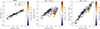 |
Fig. 5. Scaling relations of galaxies the baryonic Tully–Fisher relation (left panel), the baryonic mass–size relation (middle panel), and the baryonic angular-momentum relation (right panel). The three panels cover the same dynamic range on the y-axis. The circles and crosses are the same as those in Fig. 4, colour-coded by the effective baryonic surface density Σ50, bar. The blue and gold solid lines are the best-fit lines for LSD galaxies and HSD galaxies, respectively. The dashed black line in the right panel shows the best-fit line considering all 147 galaxies together. |
The BTFR does not distinguish between LSD and HSD galaxies. Even if we fit the two galaxy populations separately, we recover the same best-fit relation within the uncertainties. This is in agreement with previous studies, which do not find additional correlations between the BTFR residuals and other galaxy properties (e.g. Lelli et al. 2016b, 2019; Ponomareva et al. 2018; Desmond et al. 2019; Hua et al. 2025). In particular, claims of LSB galaxies deviating from the BTFR (Mancera Piña et al. 2019; Hu et al. 2023; Du et al. 2024a; Rong et al. 2024) are very dubious because they are driven by face-on galaxies with low-quality data and/or by inappropriately comparing H I line-widths from spatially unresolved data with well-measured Vflat from rotation curves (see Lelli 2024). Empirically, the BTFR seems to have irreducible scatter, so that considering any extra variable in addition to Vf at fixed Mbar (such as Eq. (3)) would only degrade the original correlation.
The AMR displays a moderate dichotomy: HSD and LSD galaxies follow different AMRs with a small offset in normalization. This offset must be driven by differences in the baryonic mass distribution at fixed Mbar because the BTFR shows no residual correlations with size and/or surface density (cf. with Eq. (3)). This occurs not only at an ‘asymptotic’ level using Vflat, but also at a ‘local’ level using the velocity V(R) at each radius R: the various Mbar − V(R) relations display no residual correlations with size at fixed mass (Desmond et al. 2019). In other words, the dichotomy in Mbar − jbar plane is the same as the one in the Mbar − R50, bar plane, but appears less evident because the optimal variable (Vf) that gives a near-perfect correlation with Mbar is effectively multiplied by another variable (such as ℛ in Eq. (3) or R50, bar in Eq. (4)).
The moderate dichotomy in the AMR is in agreement with the results of Mancera Piña et al. (2021b), who find that gas-rich galaxies have a larger intercept than gas-poor ones. Gas fraction is known to correlate with surface brightness or surface density (see, e.g. Fig. 2), so the offset found by Mancera Piña et al. (2021b) is the same as the HSD-LSD dichotomy. Importantly, the jbar − Mbar − fgas plane proposed by Mancera Piña et al. (2021b) may be the result of a circular argument. Essentially, one takes an intrinsically thin relation (the BTFR) and convolves it with another variable (such as ℛ or R50, bar at an effective level) to obtain a new relation with increased scatter (the AMR). Next, the increased scatter in the AMR is reduced considering a fourth variable (fgas) that correlates with surface density and/or R50, bar at fixed Mbar, effectively removing the extra dependency that was introduced in building the AMR in the first place.
The previous reasoning is confirmed by a simple mathematical exercise. The ‘effective’ AMR relation is given by
 (5)
(5)
where the slope S is the sum of the slopes of the BTFR and the Mbar − R50, bar relation. By fitting LSD and HSD galaxies separately, we find that S ∼ 0.64 for LSD galaxies and ∼0.72 for HSD galaxies. These values are very similar to the best-fit slopes of the actual AMR relation (∼0.73 for LSD and ∼0.83 for HSD galaxies). Of course, the values are not exactly the same because jbar is not calculated as Vf × R50, bar but by using Eq. (2). Nevertheless, this simple exercise highlights the fact that jbar is largely set by Vf and R50, bar in typical galaxies. In other words, only two scaling relations among the BTFR, AMR, and Mbar − R50, bar are independent. The BTFR is the tightest one and shows no correlation with other galaxy properties (R50, bar, Σ50, bar, and so on), so it is appropriate to consider the BTFR as a primary relation.
In the context of galaxy formation and evolution, it is sensible to think that jbar determines Vf and R50, bar (e.g. Mo et al. 1998; Fall & Efstathiou 1980). However, taking the BTFR as a primary relation, the AMR and the Mbar − R50, bar relation must contain nearly the same empirical information. Then, from a practical perspective, the Mbar − R50, bar plane appears to be a better probe of galaxy evolution than Mbar − jbar because the two galaxy populations (HSD and LSD galaxies) are much better separated in the former one, leaving little space for ambiguity. In conclusion, among the three scaling relations, the combination of BTFR and Mbar − R50, bar seems to be the best choice to test models of galaxy formation and evolution. In particular, the challenge for ΛCDM models is to reproduce the tightness of the BTFR while having two distinct sequences in the Mbar − R50, bar plane of disk galaxies.
4.3. Connections with Milgromian dynamics
The previous discussion is largely independent of the current cosmological model and the nature of dark matter. Our findings, however, have a potential connection with Milgromian dynamics (or Modified Newtonian dynamics, MOND), a paradigm that modifies the standard laws of gravity and/or inertia rather than adding dark matter (Milgrom 1983). MOND effects occur below an acceleration scale a0 ≃ 1.2 × 10⁻¹⁰ m s−2, which is imprinted in the dynamical scaling laws of galaxies (e.g. Lelli et al. 2017; Lelli 2022). The acceleration scale a0 can be recast as a characteristic surface density scale ΣM = a0/(2πG)≃137 M⊙/pc2 (e.g. Milgrom 2016, 2024), where G is Newton’s constant.
The central density relation (CDR) of galaxies is particularly relevant in this context (Lelli et al. 2016c). The CDR links the central ‘observed’ baryonic surface density Σ0, bar with the ‘dynamical’ surface density Σ0, dyn inferred from the inner steepness of the rotation curve. The CDR is a non-linear relation that displays a knee around ΣM. Galaxies with Σ0, bar > ΣM are along the one-to-one relation, so they are baryon-dominated in the inner parts (in the Newtonian regime in a MOND context). Galaxies with Σ0, bar < ΣM systematically deviate from the one-to-one line, so they are progressively more and more DM-dominated in the inner parts (in the Milgromian regime in a MOND context).
Interestingly, the division between HSD and LSD galaxies (Σc ≃ 125 M⊙/pc2) from the baryonic mass–size plane is practically indistinguishable from the characteristic MOND surface density ΣM ≃ 137 M⊙/pc2. Approximately, using the adequate mass-to-light conversions, this corresponds to the historical Freeman’s limit for the central surface brightness of galaxy disks (Freeman 1970). This fact is quite remarkable because MOND is a theory of dynamics; yet the presence of a0 is also imprinted on the structural properties of galaxies, such as the baryonic mass–size relation and the baryonic surface density distribution, which do not involve any kinematic measurement.
In the MOND context, the HSD-LSD dichotomy may naturally arise because the theory has a characteristic surface density scale, ΣM, which distinguishes between different physical regimes. Galaxies (or proto-galaxies) with Σ50, bar ≳ ΣM are in the Newtonian regime in the inner regions (with no dark matter), so they are prone to bar-like instabilities (Ostriker & Peebles 1973). By internal disk evolution, they will increase their central surface densities until they possibly reach a near-stable configuration due to the formation of bars and pseudo-bulges (Combes 2014; Nagesh et al. 2023). Thus, galaxy disks with Σ50, bar ≃ ΣM would necessarily be rare because they have evolved towards higher Σ50, bar, forming the HSD sequence. On the other hand, galaxy disks with Σ50, bar < ΣM are in the deep MOND regime, which increases their stability. These galaxies will form the LSD sequence and remain there for most of their lifetime, consuming gas in a slow, inefficient fashion (unless some external mechanisms alter their internal stability). Thus, LSD galaxies are expected to have low SFRs and low metallicities, as observed (e.g. Bothun et al. 1997). For LSD galaxies, the mean value of Σ50, bar ≃ 10 − 15 M⊙ pc−2 must then be set by the hydrodynamical properties of atomic gas, rather than by stellar dynamics. Large sets of hydrodynamical simulations of galaxy formation in MOND (e.g. Combes 2014; Wittenburg et al. 2020; Nagesh et al. 2023) are necessary to further test these ideas.
This evolutionary scenario may be closely related to the initial baryonic angular momentum in MOND. As pointed out by Milgrom (2021), MOND defines a fiducial specific angular momentum that depends on the baryonic mass of the galaxy:
 (6)
(6)
A proto-galaxy with mass Mbar and jbar ≫ jM will settle into a LSD disk. Instead, a proto-galaxy with mass Mbar but jbar ≲ jM will settle into a HSD disk with Mdisk = (jbar/jM)Mbar and develop a low-j component (such as a pseudo-bulge) that takes up the rest of the mass. In addition, Milgrom (2021) shows that
 (7)
(7)
where Σdisk is the mean surface density of the baryonic disks, which can be approximated by Σ50, disk within a factor of O(1).
Our results are in overall agreement with the MOND predictions. First, HSD disks are systematically below the AMR relation defined by LSD disks (Fig. 5, right panel). Second, gas-dominated LSD disks in our sample have Σ50, bar ≃ 0.1ΣM (Fig. 4), so MOND predicts that their AMR relation should have a slope of 3/4 = 0.75, which is entirely consistent with the best-fit slope of 0.72 ± 0.02. For star-dominated HSD disks, instead, the slope of the AMR relation (0.83 ± 0.06) seems to deviate from the MOND prediction, but the situation is more difficult to quantitatively assess. There are two main reasons: (1) HSD disks are mostly made of stars, so the computation of jbar is a very rough approximation because we do not have access to the actual stellar kinematics (through spectroscopic observations), but we use H I rotation curves to infer the stellar rotation and stellar angular momentum assuming an average pressure term in the Jeans equations (similarly to Posti et al. 2018); (2) HSD disks must undergo a redistribution of their angular momentum through secular evolution due to the formation of bars and pseudo-bulges, so the modelling of these components in the computation of jbar and Σ50, disk becomes critical; for example, our bulge-disk decompositions assign bars and pseudo-bulges to the disk (because they are expected to have a similar stellar mass-to-light ratios) so they are included in jbar and Σ50, disk, which is different from the definitions given by Milgrom (2021).
5. Conclusion
We introduced the baryonic mass–size relation of SPARC galaxies, which links the total baryonic mass (stars plus gas) with the baryonic half-mass radius. We find the following results:
-
SPARC galaxies follow two distinct sequences in the Mbar − R50, bar plane: one defined by HSD, star-dominated, Sa-Sc galaxies and one defined by LSD, gas-dominated, Sd-dI galaxies. The two sequences, which are evident by eye, are confirmed by the clustering algorithm DBSCAN.
-
The baryonic mass–size relation of LSD galaxies has a slope close to 2, pointing to a constant average baryonic surface density of the order of 10–15 M⊙ pc−2. The baryonic mass–size relation of HSD galaxies has a slope close to 1, indicating that less massive spirals are progressively more compact. The same results hold if we consider baryonic disk-only relations, excluding stellar bulges from the computation.
-
The HSD-LSD dichotomy is totally absent in the baryonic Tully–Fisher relation (Mbar versus Vflat) but moderately seen in the angular–momentum relation (Mbar versus Vflat × R50, bar), so it is driven by variations in the baryonic distribution (R50, bar) at fixed baryonic mass. This fact indicates that these relations are not independent, and that the baryonic mass–size relation provides a more incisive probe of evolutionary differences rather than the angular-momentum relation.
Our results confirm the early findings of Schombert (2006) for a different galaxy sample. In addition, the HSD-LSD dichotomy is in line with previous studies that found a dichotomy in terms of the disk central surface brightness (Tully & Verheijen 1997; Sorce et al. 2013, 2016). To put these results on firmer grounds, we are currently building a much larger sample of galaxies with both spatially resolved H I data and NIR photometry (BIG-SPARC, Haubner et al. 2024).
In a companion paper (Hua et al., in prep.), we show how studying the baryonic mass–size relation in conjunction with the stellar mass–size relation provides key insights in possible morphological transformations between star-forming and passive galaxies. In particular, we add passive galaxies (ellipticals, lenticulars, dwarf ellipticals, and dwarf spheroidals) to the current sample to obtain a global view on galaxy evolution.
The SPARC database contains three S0s (NGC 4138, UGC 2487, UGC 6786) that are detected in the ultraviolet and/or in the Hα line, suggesting recent star formation. For simplicity, in the following, we consider them as early-type spirals (Sa-Sc).
Acknowledgments
The authors thank Konstantin Haubner and Illaria Ruffa for constructive discussions during this study. EDT was supported by the European Research Council (ERC) under grant agreement no. 101040751.
References
- Afanasiev, A. V., Mei, S., Fu, H., et al. 2023, A&A, 670, A95 [NASA ADS] [CrossRef] [EDP Sciences] [Google Scholar]
- Barbieri, C. V., Fraternali, F., Oosterloo, T., et al. 2005, A&A, 439, 947 [NASA ADS] [CrossRef] [EDP Sciences] [Google Scholar]
- Bartlett, D. J., & Desmond, H. 2023, ArXiv e-prints [arXiv:2309.00948] [Google Scholar]
- Begeman, K. G. 1987, PhD thesis, University of Groningen, Kapteyn Astronomical Institute [Google Scholar]
- Begum, A., & Chengalur, J. N. 2004, A&A, 424, 509 [NASA ADS] [CrossRef] [EDP Sciences] [Google Scholar]
- Begum, A., Chengalur, J. N., & Hopp, U. 2003, New Astron., 8, 267 [Google Scholar]
- Begum, A., Chengalur, J. N., & Karachentsev, I. D. 2005, A&A, 433, L1 [NASA ADS] [CrossRef] [EDP Sciences] [Google Scholar]
- Bernardi, M., Meert, A., Vikram, V., et al. 2014, MNRAS, 443, 874 [NASA ADS] [CrossRef] [Google Scholar]
- Boomsma, R., Oosterloo, T. A., Fraternali, F., van der Hulst, J. M., & Sancisi, R. 2008, A&A, 490, 555 [NASA ADS] [CrossRef] [EDP Sciences] [Google Scholar]
- Bothun, G., Impey, C., & McGaugh, S. 1997, PASP, 109, 745 [NASA ADS] [CrossRef] [Google Scholar]
- Broeils, A. H. 1992, PhD thesis, University of Groningen, Netherlands [Google Scholar]
- Broeils, A. H., & Rhee, M. H. 1997, A&A, 324, 877 [NASA ADS] [Google Scholar]
- Calette, A. R., Avila-Reese, V., Rodríguez-Puebla, A., Hernández-Toledo, H., & Papastergis, E. 2018, Rev. Mex. Astron. Astrofis., 54, 443 [NASA ADS] [Google Scholar]
- Carignan, C., & Beaulieu, S. 1989, ApJ, 347, 760 [NASA ADS] [CrossRef] [Google Scholar]
- Carignan, C., & Puche, D. 1990a, AJ, 100, 394 [NASA ADS] [CrossRef] [Google Scholar]
- Carignan, C., & Puche, D. 1990b, AJ, 100, 641 [Google Scholar]
- Carignan, C., Sancisi, R., & van Albada, T. S. 1988, AJ, 95, 37 [Google Scholar]
- Chemin, L., Carignan, C., Drouin, N., & Freeman, K. C. 2006, AJ, 132, 2527 [Google Scholar]
- Combes, F. 2014, A&A, 571, A82 [NASA ADS] [CrossRef] [EDP Sciences] [Google Scholar]
- Cortese, L., Catinella, B., & Janowiecki, S. 2017, ApJ, 848, L7 [NASA ADS] [CrossRef] [Google Scholar]
- Côté, S., Carignan, C., & Freeman, K. C. 2000, AJ, 120, 3027 [CrossRef] [Google Scholar]
- Cote, S., Carignan, C., & Sancisi, R. 1991, AJ, 102, 904 [Google Scholar]
- de Blok, W. J. G., & McGaugh, S. S. 1997, MNRAS, 290, 533 [NASA ADS] [CrossRef] [Google Scholar]
- de Blok, W. J. G., McGaugh, S. S., & van der Hulst, J. M. 1996, MNRAS, 283, 18 [NASA ADS] [CrossRef] [Google Scholar]
- de Blok, W. J. G., Healy, J., Maccagni, F. M., et al. 2024, A&A, 688, A109 [NASA ADS] [CrossRef] [EDP Sciences] [Google Scholar]
- de Vaucouleurs, G. 1948, Ann. d’Astrophys., 11, 247 [Google Scholar]
- Desmond, H., Katz, H., Lelli, F., & McGaugh, S. 2019, MNRAS, 484, 239 [Google Scholar]
- Du, L., Du, W., Cheng, C., et al. 2024a, ApJ, 964, 85 [NASA ADS] [CrossRef] [Google Scholar]
- Du, M., Ma, H.-C., Zhong, W.-Y., et al. 2024b, A&A, 686, A168 [NASA ADS] [CrossRef] [EDP Sciences] [Google Scholar]
- Duey, F., Schombert, J., McGaugh, S., & Lelli, F. 2025, AJ, 169, 186 [Google Scholar]
- Dutton, A. A., van den Bosch, F. C., Dekel, A., & Courteau, S. 2007, ApJ, 654, 27 [NASA ADS] [CrossRef] [Google Scholar]
- Ester, M., Kriegel, H. P., Sander, J., et al. 1996, A Density-Based Algorithm for Discovering Clusters in Large Spatial Databases with Noise, 226 [Google Scholar]
- Fall, S. M. 1983, in Internal Kinematics and Dynamics of Galaxies, ed. E. Athanassoula, IAU Symp., 100, 391 [Google Scholar]
- Fall, S. M., & Efstathiou, G. 1980, MNRAS, 193, 189 [NASA ADS] [CrossRef] [Google Scholar]
- Fernández Lorenzo, M., Sulentic, J., Verdes-Montenegro, L., & Argudo-Fernández, M. 2013, MNRAS, 434, 325 [Google Scholar]
- Frank, B. S., de Blok, W. J. G., Walter, F., Leroy, A., & Carignan, C. 2016, AJ, 151, 94 [NASA ADS] [CrossRef] [Google Scholar]
- Fraternali, F., Sancisi, R., & Kamphuis, P. 2011, A&A, 531, A64 [NASA ADS] [CrossRef] [EDP Sciences] [Google Scholar]
- Freeman, K. C. 1970, ApJ, 160, 811 [Google Scholar]
- Gadotti, D. A. 2009, MNRAS, 393, 1531 [Google Scholar]
- Gault, L., Leisman, L., Adams, E. A. K., et al. 2021, ApJ, 909, 19 [NASA ADS] [CrossRef] [Google Scholar]
- Gentile, G., Salucci, P., Klein, U., Vergani, D., & Kalberla, P. 2004, MNRAS, 351, 903 [Google Scholar]
- Greene, J. E., Greco, J. P., Goulding, A. D., et al. 2022, ApJ, 933, 150 [NASA ADS] [CrossRef] [Google Scholar]
- Hallenbeck, G., Huang, S., Spekkens, K., et al. 2014, AJ, 148, 69 [NASA ADS] [CrossRef] [Google Scholar]
- Haubner, K., Lelli, F., Di Teodoro, E., et al. 2024, ArXiv e-prints [arXiv:2411.13329] [Google Scholar]
- Hu, H.-J., Guo, Q., Zheng, Z., et al. 2023, ApJ, 947, L9 [NASA ADS] [CrossRef] [Google Scholar]
- Hua, Z., Rong, Y., & Hu, H. 2025, MNRAS, 538, 775 [Google Scholar]
- Huang, K.-H., Fall, S. M., Ferguson, H. C., et al. 2017, ApJ, 838, 6 [NASA ADS] [CrossRef] [Google Scholar]
- Jobin, M., & Carignan, C. 1990, AJ, 100, 648 [Google Scholar]
- Kepley, A. A., Wilcots, E. M., Hunter, D. A., & Nordgren, T. 2007, AJ, 133, 2242 [NASA ADS] [CrossRef] [Google Scholar]
- Kim, J.-H., & Lee, J. 2013, MNRAS, 432, 1701 [Google Scholar]
- Kim, Y., & Kim, W.-T. 2014, MNRAS, 440, 208 [NASA ADS] [CrossRef] [Google Scholar]
- Kravtsov, A. V. 2013, ApJ, 764, L31 [NASA ADS] [CrossRef] [Google Scholar]
- Lake, G., Schommer, R. A., & van Gorkom, J. H. 1990, AJ, 99, 547 [Google Scholar]
- Lange, R., Driver, S. P., Robotham, A. S. G., et al. 2015, MNRAS, 447, 2603 [CrossRef] [Google Scholar]
- Lelli, F. 2022, Nat. Astron., 6, 35 [NASA ADS] [CrossRef] [Google Scholar]
- Lelli, F. 2024, A&A, 689, L3 [NASA ADS] [CrossRef] [EDP Sciences] [Google Scholar]
- Lelli, F., Verheijen, M., & Fraternali, F. 2014, A&A, 566, A71 [NASA ADS] [CrossRef] [EDP Sciences] [Google Scholar]
- Lelli, F., McGaugh, S. S., & Schombert, J. M. 2016a, AJ, 152, 157 [Google Scholar]
- Lelli, F., McGaugh, S. S., & Schombert, J. M. 2016b, ApJ, 816, L14 [Google Scholar]
- Lelli, F., McGaugh, S. S., Schombert, J. M., & Pawlowski, M. S. 2016c, ApJ, 827, L19 [NASA ADS] [CrossRef] [Google Scholar]
- Lelli, F., McGaugh, S. S., Schombert, J. M., & Pawlowski, M. S. 2017, ApJ, 836, 152 [Google Scholar]
- Lelli, F., McGaugh, S. S., Schombert, J. M., Desmond, H., & Katz, H. 2019, MNRAS, 484, 3267 [NASA ADS] [CrossRef] [Google Scholar]
- Leroy, A. K., Walter, F., Brinks, E., et al. 2008, AJ, 136, 2782 [Google Scholar]
- Liao, S., Gao, L., Frenk, C. S., et al. 2019, MNRAS, 490, 5182 [NASA ADS] [CrossRef] [Google Scholar]
- Lin, C. C., & Shu, F. H. 1964, ApJ, 140, 646 [Google Scholar]
- Lutz, K. A., Kilborn, V. A., Koribalski, B. S., et al. 2018, MNRAS, 476, 3744 [NASA ADS] [CrossRef] [Google Scholar]
- Mancera Piña, P. E., Fraternali, F., Adams, E. A. K., et al. 2019, ApJ, 883, L33 [CrossRef] [Google Scholar]
- Mancera Piña, P. E., Posti, L., Fraternali, F., Adams, E. A. K., & Oosterloo, T. 2021a, A&A, 647, A76 [NASA ADS] [CrossRef] [EDP Sciences] [Google Scholar]
- Mancera Piña, P. E., Posti, L., Pezzulli, G., et al. 2021b, A&A, 651, L15 [NASA ADS] [CrossRef] [EDP Sciences] [Google Scholar]
- Marasco, A., de Blok, W. J. G., Maccagni, F. M., et al. 2025, A&A, 697, A86 [NASA ADS] [CrossRef] [EDP Sciences] [Google Scholar]
- McDonald, M., Courteau, S., & Tully, R. B. 2009a, MNRAS, 393, 628 [Google Scholar]
- McDonald, M., Courteau, S., & Tully, R. B. 2009b, MNRAS, 394, 2022 [Google Scholar]
- McGaugh, S. S. 2005, Phys. Rev. Lett., 95, 171302 [NASA ADS] [CrossRef] [Google Scholar]
- McGaugh, S. S., Schombert, J. M., Bothun, G. D., & de Blok, W. J. G. 2000, ApJ, 533, L99 [Google Scholar]
- McGaugh, S. S., Schombert, J. M., & Lelli, F. 2017, ApJ, 851, 22 [Google Scholar]
- McGaugh, S. S., Lelli, F., & Schombert, J. M. 2020, Res. Notes Am. Astron. Soc., 4, 45 [Google Scholar]
- Milgrom, M. 1983, ApJ, 270, 371 [Google Scholar]
- Milgrom, M. 2016, Phys. Rev. Lett., 117, 141101 [Google Scholar]
- Milgrom, M. 2021, Phys. Rev. D, 104, 064030P [Google Scholar]
- Milgrom, M. 2024, Phys. Rev. D, 109, 124016P [Google Scholar]
- Mo, H. J., Mao, S., & White, S. D. M. 1998, MNRAS, 295, 319 [Google Scholar]
- Mowla, L. A., van Dokkum, P., Brammer, G. B., et al. 2019, ApJ, 880, 57 [NASA ADS] [CrossRef] [Google Scholar]
- Nagesh, S. T., Kroupa, P., Banik, I., et al. 2023, MNRAS, 519, 5128 [NASA ADS] [CrossRef] [Google Scholar]
- Nedkova, K. V., Häußler, B., Marchesini, D., et al. 2024, MNRAS, 532, 3747 [Google Scholar]
- Noordermeer, E., van der Hulst, J. M., Sancisi, R., Swaters, R. A., & van Albada, T. S. 2005, A&A, 442, 137 [NASA ADS] [CrossRef] [EDP Sciences] [Google Scholar]
- Ostriker, J. P., & Peebles, P. J. E. 1973, ApJ, 186, 467 [Google Scholar]
- Pedregosa, F., Varoquaux, G., Gramfort, A., et al. 2011, J. Mach. Learn. Res., 12, 2825 [Google Scholar]
- Peschken, N., & Łokas, E. L. 2019, MNRAS, 483, 2721 [Google Scholar]
- Ponomareva, A. A., Verheijen, M. A. W., Papastergis, E., Bosma, A., & Peletier, R. F. 2018, MNRAS, 474, 4366 [Google Scholar]
- Posti, L., Fraternali, F., Di Teodoro, E. M., & Pezzulli, G. 2018, A&A, 612, L6 [NASA ADS] [CrossRef] [EDP Sciences] [Google Scholar]
- Puche, D., Carignan, C., & Wainscoat, R. J. 1991, AJ, 101, 447 [Google Scholar]
- Querejeta, M., Leroy, A. K., Meidt, S. E., et al. 2024, A&A, 687, A293 [NASA ADS] [CrossRef] [EDP Sciences] [Google Scholar]
- Ramón-Fox, F. G., & Aceves, H. 2020, MNRAS, 491, 3908 [CrossRef] [Google Scholar]
- Rhee, M. H., & van Albada, T. S. 1996, A&AS, 115, 407 [Google Scholar]
- Richards, E. E., van Zee, L., Barnes, K. L., et al. 2015, MNRAS, 449, 3981 [NASA ADS] [CrossRef] [Google Scholar]
- Richards, E. E., van Zee, L., Barnes, K. L., et al. 2016, MNRAS, 460, 689 [Google Scholar]
- Roberts, W. W. 1969, ApJ, 158, 123 [NASA ADS] [CrossRef] [Google Scholar]
- Robotham, A. S. G., & Obreschkow, D. 2015, PASA, 32, e033 [Google Scholar]
- Rodriguez, F., Montero-Dorta, A. D., Angulo, R. E., Artale, M. C., & Merchán, M. 2021, MNRAS, 505, 3192 [NASA ADS] [CrossRef] [Google Scholar]
- Roelfsema, P. R., & Allen, R. J. 1985, A&A, 146, 213 [NASA ADS] [Google Scholar]
- Romanowsky, A. J., & Fall, S. M. 2012, ApJS, 203, 17 [Google Scholar]
- Rong, Y., Guo, Q., Gao, L., et al. 2017, MNRAS, 470, 4231 [Google Scholar]
- Rong, Y., Hu, H., He, M., et al. 2024, ArXiv e-prints [arXiv:2404.00555] [Google Scholar]
- Roy, N., Napolitano, N. R., La Barbera, F., et al. 2018, MNRAS, 480, 1057 [Google Scholar]
- Saintonge, A., & Catinella, B. 2022, ARA&A, 60, 319 [NASA ADS] [CrossRef] [Google Scholar]
- Sancisi, R., Fraternali, F., Oosterloo, T., & van der Hulst, T. 2008, A&ARv, 15, 189 [NASA ADS] [CrossRef] [Google Scholar]
- Schombert, J., McGaugh, S., & Lelli, F. 2019, MNRAS, 483, 1496 [NASA ADS] [Google Scholar]
- Schombert, J., McGaugh, S., & Lelli, F. 2022, AJ, 163, 154 [NASA ADS] [CrossRef] [Google Scholar]
- Schombert, J. M. 2006, AJ, 131, 296 [Google Scholar]
- Sellwood, J. A. 2014, Rev. Mod. Phys., 86, 1 [Google Scholar]
- Sellwood, J. A., & Masters, K. L. 2022, ARA&A, 60 [Google Scholar]
- Sérsic, J. L. 1963, Boletin de la Asociacion Argentina de Astronomia La Plata Argentina, 6, 41 [Google Scholar]
- Shen, S., Mo, H. J., White, S. D. M., et al. 2003, MNRAS, 343, 978 [NASA ADS] [CrossRef] [Google Scholar]
- Somerville, R. S., Behroozi, P., Pandya, V., et al. 2018, MNRAS, 473, 2714 [NASA ADS] [CrossRef] [Google Scholar]
- Sorce, J. G., Courtois, H. M., Sheth, K., & Tully, R. B. 2013, MNRAS, 433, 751 [Google Scholar]
- Sorce, J. G., Creasey, P., & Libeskind, N. I. 2016, MNRAS, 455, 2644 [Google Scholar]
- Spekkens, K., & Giovanelli, R. 2006, AJ, 132, 1426 [Google Scholar]
- Starkman, N., Lelli, F., McGaugh, S., & Schombert, J. 2018, MNRAS, 480, 2292 [Google Scholar]
- Stevens, A. R. H., Diemer, B., Lagos, C. D. P., et al. 2019, MNRAS, 490, 96 [Google Scholar]
- Swaters, R. A., van Albada, T. S., van der Hulst, J. M., & Sancisi, R. 2002, A&A, 390, 829 [NASA ADS] [CrossRef] [EDP Sciences] [Google Scholar]
- Trujillo, I., Chamba, N., & Knapen, J. H. 2020, MNRAS, 493, 87 [NASA ADS] [CrossRef] [Google Scholar]
- Tully, R. B., & Verheijen, M. A. W. 1997, ApJ, 484, 145 [NASA ADS] [CrossRef] [Google Scholar]
- van Albada, T. S., & Sancisi, R. 1986, Phil. Trans. Royal Soc. London Ser. A, 320, 447 [Google Scholar]
- van der Hulst, J. M., Skillman, E. D., Smith, T. R., et al. 1993, AJ, 106, 548 [NASA ADS] [CrossRef] [Google Scholar]
- van der Wel, A., Franx, M., van Dokkum, P. G., et al. 2014, ApJ, 788, 28 [Google Scholar]
- van Zee, L. 2001, AJ, 121, 2003 [NASA ADS] [CrossRef] [Google Scholar]
- van Zee, L., Haynes, M. P., Salzer, J. J., & Broeils, A. H. 1997, AJ, 113, 1618 [Google Scholar]
- Verdes-Montenegro, L., Bosma, A., & Athanassoula, E. 1997, A&A, 321, 754 [NASA ADS] [Google Scholar]
- Verheijen, M. A. W., & Sancisi, R. 2001, A&A, 370, 765 [NASA ADS] [CrossRef] [EDP Sciences] [Google Scholar]
- Vogelaar, M. G. R., & Terlouw, J. P. 2001, in Astronomical Data Analysis Software and Systems X, eds. F. R. Harnden, Jr., F. A. Primini, & H. E. Payne, ASP Conf. Ser., 238, 358 [NASA ADS] [Google Scholar]
- Walsh, W., Staveley-Smith, L., & Oosterloo, T. 1997, AJ, 113, 1591 [Google Scholar]
- Wang, J., Koribalski, B. S., Serra, P., et al. 2016, MNRAS, 460, 2143 [Google Scholar]
- Wittenburg, N., Kroupa, P., & Famaey, B. 2020, ApJ, 890, 173 [NASA ADS] [CrossRef] [Google Scholar]
- Wyder, T. K., Martin, D. C., Barlow, T. A., et al. 2009, ApJ, 696, 1834 [NASA ADS] [CrossRef] [Google Scholar]
- Yang, L., Roberts-Borsani, G., Treu, T., et al. 2021, MNRAS, 501, 1028 [Google Scholar]
- Yu, S.-Y., Ho, L. C., & Wang, J. 2021, ApJ, 917, 88 [NASA ADS] [CrossRef] [Google Scholar]
Appendix A: Tables
In section 2, we described the compilation of H I surface density profiles for 169 galaxies. References for the H I data and the corresponding number of galaxies are listed in Table A.1.
In section 3, we used the ROXY software to fit the baryonic mass–size relations of HSD and LSD galaxies separately. Table A.2 provides the best-fit parameters of the Mbar − R50, bar relation, considering different physical properties to divide the two groups of galaxies. Table A.3 provides the same information for the Mdisk − R50, disk relation, in which stellar bulges are excluded.
In Section 4, we used the ROXY software to fit the baryonic Tully-Fisher relation, the baryonic mass–size relation (switching the axes with respect to Sect. 3), and the baryonic angular momentum relation for HSD and LSD galaxies separately. Table A.4 provides the best-fit parameters.
References for the H I surface density profiles
ROXY best-fit parameters for the R50, bar − Mbar relations, dividing SPARC galaxies in two groups based on Σ50, bar (our fiducial distinction between HSD and LSD galaxies), fgas, and T.
ROXY best-fit parameters for the R50, disk − Mdisk relations, dividing SPARC galaxies in two groups based on Σ50, bar (our fiducial distinction between HSD and LSD galaxies), fgas, and T.
ROXY best-fit parameters of the baryonic Tully-Fisher relation, baryonic mass–size relation, and baryonic angular-momentum relation fitting LSD galaxies (left columns) and HSD galaxies (right columns) separately.
Appendix B: Error estimation
Following Lelli et al. (2016b), we estimated the error on Mbar as
 (B.1)
(B.1)
where δFHI is the uncertainty on the H I flux (about 10%), δL is the uncertainty on the 3.6 μm luminosity (a few per cent), δΥ* is the uncertainty on the stellar mass-to-light ratio (dominated by galaxy-to-galaxy variations that are assumed to be of ∼25%), and δD is the uncertainty on the galaxy distance (varying from 5% to 30% depending on the galaxy, see Lelli et al. 2016a). When a galaxy bulge is present, the third term inside the square root was replaced by two similar terms: one for the stellar disk and one for the stellar bulge. The error on the disk mass (excluding the bulge) was given by the same equation by replacing M⋆ with the mass of the stellar disk and Mbar with the mass of the baryonic disk.
The errors on R50, bar were estimated as
 (B.2)
(B.2)
where θ50 is half-mass radius in arcsec. We assumed that δθ50/θ50 = 1/n, where n is the number of H I spatially resolved elements along the disk semi-major axis (approximately the number of points along the SPARC rotation curve).
In logarithmic space, the covariance between δMbar and δR50, bar is given by
 (B.3)
(B.3)
The values of Vf and the corresponding errors are taken directly from Lelli et al. (2019). For galaxies without a measured Vf, we considered the last point of the rotation curve and the corresponding error (accounting for uncertainties on inclination too). Vf does not depend on D, so there is no need to consider the covariance matrix between Mbar and Vf.
The error on jbar is estimated following Mancera Piña et al. (2021b). The covariance between Mbar and jbar (in logarithmic space) can be roughly estimated as,
 (B.4)
(B.4)
according to equation (4). Nevertheless, we find that even if we do not include the covariant term σMbarjbar, the best-fitting results do not change significantly.
Appendix C: Results using different fitting codes
In Section 3.2, we determined the best-fit parameters of the R50, bar − Mbar relation using the ROXY software, which fits for the vertical intrinsic scatter (‘vertical fitting’). It is known that the results produced by vertical and orthogonal fittings can have considerable differences (see Appendix A of Lelli et al. 2019), so we repeated the fits using the codes BAYESLINEFIT (Lelli et al. 2019) and HYPERFIT (Robotham & Obreschkow 2015), both of which allow for orthogonal fitting.
The results are provided in Tables C.1 and C.2, respectively. Both orthogonal fitting codes yield larger slopes than those given by the vertical fitting code ROXY, in agreement with the results of Lelli et al. (2019). In general, it is not obvious to decide whether vertical fitting is preferable to orthogonal fitting (or vice versa). In this paper, we adopted the results from vertical fitting because ROXY has been amply tested using mock datasets and seems to provide unbiased results (Bartlett & Desmond 2023).
Finally, we note that the best-fit parameters from HYPERFIT and BAYESLINEFIT are consistent with each other within 1σ, albeit the former takes the covariance matrix of each data point into account whereas the latter does not. This confirms that the covariance matrix has a minor effect on the best-fit results.
BAYESLINEFIT best-fit parameters of the R50, bar − Mbar relations, dividing SPARC galaxies in two groups based on Σ50, bar (our fiducial distinction between HSD and LSD galaxies), fgas, and T.
HYPERFIT best-fit parameters of the R50, bar − Mbar relations, dividing SPARC galaxies in two groups based on Σ50, bar (our fiducial distinction between HSD and LSD galaxies), fgas, and T.
All Tables
ROXY best-fit parameters for the R50, bar − Mbar relations, dividing SPARC galaxies in two groups based on Σ50, bar (our fiducial distinction between HSD and LSD galaxies), fgas, and T.
ROXY best-fit parameters for the R50, disk − Mdisk relations, dividing SPARC galaxies in two groups based on Σ50, bar (our fiducial distinction between HSD and LSD galaxies), fgas, and T.
ROXY best-fit parameters of the baryonic Tully-Fisher relation, baryonic mass–size relation, and baryonic angular-momentum relation fitting LSD galaxies (left columns) and HSD galaxies (right columns) separately.
BAYESLINEFIT best-fit parameters of the R50, bar − Mbar relations, dividing SPARC galaxies in two groups based on Σ50, bar (our fiducial distinction between HSD and LSD galaxies), fgas, and T.
HYPERFIT best-fit parameters of the R50, bar − Mbar relations, dividing SPARC galaxies in two groups based on Σ50, bar (our fiducial distinction between HSD and LSD galaxies), fgas, and T.
All Figures
|
Fig. 1. Measurements of R50, gas, R50, ⋆, and R50, bar for three example galaxies: a gas-dominated one (UGC 731), a star-dominated one (NGC 2903), and an intermediate case (NGC 5585). The upper panels show the surface density profiles for gas (blue points), stars (red points), and total baryons (black line); the stellar profile was extrapolated at large radii with an exponential function (dashed red line). The lower panel shows the curve of growth of gas (blue line), stars (red line), and total baryons (black line); the dotted lines show the location of the corresponding half-mass radii. |
| In the text | |
|
Fig. 2. Gaseous (left panel), stellar (middle panel), and baryonic (right panel) mass–size relations of SPARC galaxies. Data points are colour-coded by the gas fraction fgas; the error bars denote the 1σ errors. The three panels span the same dynamic range on both axes. Two sequences are evident in the stellar and baryonic mass–size relations. |
| In the text | |
|
Fig. 3. Distributions of fgas, Σ50, bar, T, and μ0, disk for the two groups identified by DBSCAN (red and blue histograms). The dashed black lines show the separation values reported in Table A.2. Panels (a)–(c) show the distributions clustered by logΣ50, bar, while panel (d) shows the distributions clustered by μ0, disk (after correction to a face-on view). |
| In the text | |
|
Fig. 4. Baryonic mass–size relations considering all baryons (left panel) and the baryonic disks only (excluding stellar bulges, right panel). Galaxies are colour-coded by the gas fraction fgas. Crosses represent S0-to-Sc galaxies (Hubble type T ≤ 5), while circles represent Sd-to-dI galaxies (T > 5). The red and the blue solid lines show the best-fit relations to the HSD and LSD sequences, respectively; the red and blue shaded areas indicate the best-fit intrinsic scatters. Dashed lines correspond to constant surface densities for multiples of Σc = 125 M⊙ pc−2 (see Sect. 3 for details). |
| In the text | |
|
Fig. 5. Scaling relations of galaxies the baryonic Tully–Fisher relation (left panel), the baryonic mass–size relation (middle panel), and the baryonic angular-momentum relation (right panel). The three panels cover the same dynamic range on the y-axis. The circles and crosses are the same as those in Fig. 4, colour-coded by the effective baryonic surface density Σ50, bar. The blue and gold solid lines are the best-fit lines for LSD galaxies and HSD galaxies, respectively. The dashed black line in the right panel shows the best-fit line considering all 147 galaxies together. |
| In the text | |
Current usage metrics show cumulative count of Article Views (full-text article views including HTML views, PDF and ePub downloads, according to the available data) and Abstracts Views on Vision4Press platform.
Data correspond to usage on the plateform after 2015. The current usage metrics is available 48-96 hours after online publication and is updated daily on week days.
Initial download of the metrics may take a while.