| Issue |
A&A
Volume 703, November 2025
|
|
|---|---|---|
| Article Number | A212 | |
| Number of page(s) | 12 | |
| Section | Planets, planetary systems, and small bodies | |
| DOI | https://doi.org/10.1051/0004-6361/202555854 | |
| Published online | 18 November 2025 | |
Simulation of impact-induced seismic shaking on asteroid (25143) Itokawa to address its resurfacing process
1
Department of Physics and Astronomy, Seoul National University,
1 Gwanak-ro,
Gwanak-gu, Seoul
08826,
Republic of Korea
2
SNU Astronomy Research Center, Department of Physics and Astronomy, Seoul National University,
1 Gwanak-ro,
Gwanak-gu, Seoul
08826,
Republic of Korea
3
Korea Astronomy and Space Science Institute (KASI),
776 Daedeok-daero,
Yuseong-gu, Daejeon
34055,
Republic of Korea
★ Corresponding authors: sjin@kasi.re.kr; ishiguro@snu.ac.kr
Received:
6
June
2025
Accepted:
8
September
2025
Context. The surface of asteroid (25143) Itokawa shows both fresh and mature terrains, despite its short space-weathering timescale of approximately 103 years, as inferred from recent studies. Seismic shaking triggered by the impact that formed the 8-meter crater Kamoi has been proposed as a possible explanation for the diversity.
Aims. This study aims to examine whether the seismic shaking induced by the impact might account for the observed spatial variations in space weathering and might further constrain the internal structure of Itokawa.
Methods. Assuming that the Kamoi crater was formed by a recent impact, we conducted three-dimensional seismic wave propagation simulations and applied a simplified landslide model to estimate surface accelerations and boulder displacements.
Results. Our results show that even a low-energy case (1% of the nominal seismic energy) produces surface accelerations sufficient to destabilize the surface materials. The simulated boulder displacements are consistent with the observed distribution of space-weathering degrees even on the opposite hemisphere. We estimate the seismic diffusivity to be 1000–2000 m2 s−1 and the seismic efficiency to be in the range of 5.0 × 10⁻⁸ to 5.0 × 10⁻⁷, implying that the interior of Itokawa contains blocks tens of meters across and acts as a strongly scattering medium.
Conclusions. Our findings provide unique dynamical evidence, based on seismic wave propagation modeling, that supports the hypothesis that the interior of Itokawa truly is a rubble pile.
Key words: minor planets, asteroids: general / minor planets, asteroids: individual: (25143) Itokawa
© The Authors 2025
 Open Access article, published by EDP Sciences, under the terms of the Creative Commons Attribution License (https://creativecommons.org/licenses/by/4.0), which permits unrestricted use, distribution, and reproduction in any medium, provided the original work is properly cited.
This article is published in open access under the Subscribe to Open model. Subscribe to A&A to support open access publication.
1 Introduction
The surfaces of airless bodies undergo various physical and chemical evolutionary processes when exposed to the space environment. One of the most significant of these processes is space weathering. It is primarily caused by solar wind implantation and micrometeorite bombardment. It alters the optical properties of the airless bodies (Pieters & Noble 2016; Chapman 2004; Clark et al. 2002). This process has been observed on several celestial bodies, including the Moon (Pieters et al. 2000), Mercury (Hapke 2001), and many asteroids (Clark et al. 2002). In particular, for S-type near-Earth asteroids, space weathering is known to reduce albedo, redden the spectral slope, and reduce the absorption depth near 1 µm (see e.g. Sasaki et al. 2001).
The Hayabusa mission target, asteroid (25143) Itokawa, exhibits a unique appearance characterized by a wide range of space-weathering degrees across its surface. A puzzling discrepancy exists in the estimated timescales of the weathering on Itokawa, however, which ranges from 102 to 107 years (Bonal et al. 2015; Koga et al. 2018; Noguchi 2011; Keller & Berger 2014; Matsumoto et al. 2018; Nagao 2011). Based on analyses of returned samples, space-weathering research has made significant progress. Nagao (2011) estimated surface exposure ages of only 3000–8000 years through noble-gas analyses of returned particles. In addition, Noguchi et al. (2014) observed nanometer-scale weathered rims on the surfaces of Itokawa grains using transmission electron microscopy. This offered new insights into the microstructural development of space weathering. Our group also estimated a space-weathering timescale of approximately 103 years by analyzing the size-frequency distribution of white mottles on boulder surfaces (Jin & Ishiguro 2022). This result, based on remote-sensing data, is consistent with estimates from returned samples by Noguchi (2011), which indicated short exposure durations.
Despite the short timescale of space weathering on Itokawa, it remains unclear why several regions still display less strongly weathered surfaces. If the impact had occurred more than several tens of thousands of years ago, fresh features like this would likely have been erased by space weathering. In addition, fresh terrains are not only found near the Kamoi crater, but are also scattered across other regions, and the factors controlling this spatial distribution remain unresolved. Saito et al. (2006) noted that fresh terrains are more prevalent on the Kamoi crater side, but did not address the cause of their formation. Jin & Ishiguro (2022) proposed that the 8-meter-wide Kamoi crater may have generated seismic waves strong enough to trigger localized landslides, thereby exposing unweathered material beneath the surface. They further hypothesized that areas with large boulders may display fresh terrains due to lateral boulder movement, which might uncover pristine material underneath.
To test the hypothesis proposed by Jin & Ishiguro (2022), we conducted three-dimensional (3D) seismic wave propagation simulations and subsequent landslides resulting from the Kamoi impact. Previous studies have modeled seismic wave propagation within asteroids (e.g., Richardson et al. 2005; Quillen et al. 2019; Ballouz et al. 2024). Notably, Richardson et al. (2020) estimated crater retention ages and constrained the surface and internal properties of four asteroids, including Itokawa, by modeling topographic diffusion caused by seismic shaking. Their study employed simplified cylindrical coordinates scaled to match the surface area of each asteroid as part of a generalized approach, however, which limited the fidelity of the seismic wave propagation analysis in a realistic shape model.
We used a shape model based on remote-sensing observations of Itokawa, reconstructed from disk-resolved images taken by the Asteroid Multi-band Imaging Camera (AMICA) aboard the Hayabusa spacecraft (Gaskell 2020), to compute the seismic wave propagation within the three-dimensional geometry of the asteroid. In addition, we developed a toy model to quantitatively simulate landslides on each facet of the shape model. Based on the simulation results, we analyzed the conditions under which fresh terrains are formed on Itokawa. Furthermore, we investigated how varying physical parameters influence our results, particularly in terms of inferring the internal structure from the spatial distribution of surface space weathering.
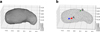 |
Fig. 1 Three-dimensional views of (a) the original shape model of Itokawa with 49 152 facets from Gaskell (2020) and (b) the simplified model with 1024 facets used in this study. The blue star denotes the location of the Kamoi crater. Red (A) and green (B) facets correspond to facets 152 and 93, respectively, and are used for comparison in Figs. 3 and 7. |
2 Method
We employed a two-step modeling approach to investigate the spatial distribution of fresh terrains on the surface of Itokawa. First, we simulated the propagation of seismic energy triggered by the impact that formed the Kamoi crater using a three-dimensional diffusion model (Section 2.1). Then, we developed a simplified landslide model to estimate the displacement of surface boulders (Sect. 2.2). The following subsections describe each step in detail.
2.1 Seismic energy propagation
We conducted a numerical simulation for the seismic energy propagation using the shape model provided by Gaskell (2020), which contains 49 152 triangular facets in its simplest form (Fig. 1a). We found that some facet slopes in the model were affected by meter-scale surface boulders and do not reflect the real slope of the asteroid surface. Therefore, we reduced the number of facets to 1024 using pymesh.meshing_decimation_quadric_edge_collapse, a function from PyMesh, a Python library for geometry processing (see Figure 1b). This function is based on the quadric error metrics algorithm (Garland & Heckbert 1997). As a result of the simplification, the average area of the simplified facets is 3.87 ± 2.09 × 10² m2, which corresponds to an effective length of 19.03 ± 4.94 m. This length is larger than that of most surface boulders, effectively minimizing the influence of individual boulders on the facet geometry (Michikami et al. 2008).
Next, we prepared a 3D grid to solve the seismic energy diffusion equation. We generated a 600 × 400 × 300 grid with a spacing of 2 m. The grid size and resolution were chosen to fully enclose the entire volume of Itokawa, whose maximum extent is approximately 535 m, within the grid. We assigned an initial value of zero to grid cells inside the shape model. Grid cells outside the shape model were assigned a placeholder value of not a number (NaN), a standard marker in numerical computations used to indicate undefined or excluded regions.
The total seismic energy Es was calculated using the following equation:
 (1)
(1)
where Ei, mi, υi, ri, and ρi are the kinetic energy, mass, velocity, radius, and mass density of the impactor, respectively. We assumed υi = 25 km s−1, ri = 20 cm, and ρi = 3 g cm−3 to reproduce an 8-m crater like Kamoi, based on the scaling relation by Tatsumi & Sugita (2018). η is an efficiency parameter, defined as the ratio of the total seismic energy and the kinetic energy of the impactor. The values of η used in the simulations are listed in Table 1. Richardson et al. (2020) estimated the seismic efficiency of Itokawa to be 1.0 ± 0.5 × 10⁻⁷.
Using the Small Body Mapping Tool (SBMT) (Ernst et al. 2018), we identified the location of the Kamoi crater as (X, Y, Z) = (−67.4, −143,15.2). We assumed that the initial seismic energy was distributed radially within 4 m from this point, weighted inversely with the squared distance. This approach provides a simple approximation of localized energy deposition near the impact site. Although not based on a detailed seismic source model, the inverse-distance method concentrates energy near the impact and alleviates edge discontinuities.
We modeled the propagation of seismic energy using a diffusion equation with an attenuation term, following the approach of Dainty et al. (1974) and Richardson et al. (2005),
 (2)
(2)
where ϵ is the seismic energy density, K is the diffusivity, f is the dominant frequency of the seismic wave, and Q is the quality factor. The diffusivity is defined as
 (3)
(3)
where υ is the seismic wave velocity, and l is the mean free path. The values of K used in the simulations are listed in Table 1. We adopted a nominal and possible range of diffusivity in Richardson et al. (2020), who reported K = 2000 m2 s−1 as a nominal value and 1000–3000 m2 s−1 as a possible range. We assumed a dominant frequency of f = 10 Hz, consistent with hydrocode simulations showing that the seismic wave energy peaks in this frequency range (Richardson et al. 2020). We adopted a constant quality factor of Q = 1500 for all cases.
We solved Eq. (2) using the fourth-order Runge–Kutta method for 10 seconds after the impact. The default time step was set to 0.001 seconds and was reduced to 0.0001 seconds for cases where K > 3000 m2 s−1 to maintain numerical stability. We applied Neumann boundary conditions (zero energy flux) to model waves reflected from the surface since the outside of the asteroid has a much lower density than the interior. This assumption likely overestimates the retained energy by ignoring losses to space, however. We discuss an effect of the boundary condition like this in Sect. 4.1. At each time step, we converted the seismic energy density ϵ into the peak acceleration amplitude a, assuming simple harmonic oscillation,
 (4)
(4)
where ρt = 1.9 g cm−3 is the bulk density of Itokawa (Fujiwara et al. 2006). This provides the acceleration envelope for monochromatic oscillation at a frequency f. Although actual seismic motion involves a broad spectrum of frequencies, we used a as a proxy for the net upward acceleration, assuming that overlapping modes constructively enhance vertical motion, as illustrated in Fig. 4b of Richardson et al. (2020).
List of simulations.
2.2 Landslide toy model
We developed a toy model to estimate the downslope motion of a boulder on each facet of the simplified shape model over 10 minutes after the impact. We considered three forces: gravity, seismic acceleration, and friction.
Gravity was modeled using the Mascon method by dividing the interior of the asteroid into tetrahedra based on 3D Delaunay triangulation, implemented in the scipy.spatial.Delaunay module of the SciPy library (Virtanen et al. 2020), with a 10 m internal grid spacing. The total number of tetrahedra (NV) was 128 672.
Previous studies reported a difference in internal density between the head and body regions of Itokawa (Lowry et al. 2014; Kanamaru et al. 2019). We adopted a density of 2450 kg m−3 for the head (X > +150 m) and 1930 kg m−3 for the body (X < +150 m) from Kanamaru et al. (2019). We then calculated a composite force vector (F) of gravity and centrifugal force acting on the centroid of each facet using the following equation:
 (5)
(5)
where G is the gravitational constant, ρi, Vi, and ri are the mass density, volume, and position vector of each volume element; r and r⊥ are the centroid position vector and perpendicular component from the spin axis; and ω is the spin rate. We used the rotational period of Itokawa of 12.1324 hours (Fujiwara et al. 2006). We defined the surface slope (θ) as the angle between the facet normal and the gravity vector.
Seismic acceleration from Sect. 2.1 was assumed to act along the normal direction of each facet. Since acceleration was computed for 10 seconds, we extrapolated the last 2 seconds over 10 minutes, assuming exponential decay. Last, we used friction coefficients (µ) from DellaGiustina et al. (2024), with 0.6 for the static and kinetic friction constants.
The motion of a surface boulder on each facet was integrated using the Euler method with a time step of 0.025 seconds, based on the assumption that a mass undergoing harmonic motion experiences peak acceleration for approximately one-quarter of its oscillation period (the inverse of f =10 Hz). At each time step, we first determined whether the boulder was located on or above the surface. If the boulder was above the surface, it was considered to be in ballistic motion and was influenced by gravity alone. We assumed a completely inelastic collision, setting the boulder velocity to zero upon impact with the slope surface. This assumption may underestimate subsequent motion after landing, such as rolling or bouncing. The implications of this assumption are discussed in Sect. 4.1.
If the boulder was on the slope, we compared the seismic acceleration a to the normal component of gravitational acceleration, 𝑔 cos θ. If a > 𝑔 cos θ, the boulder was assumed to be launched and transitioned into ballistic motion. If a < 𝑔 cos θ, we evaluated whether downslope sliding occurred by comparing the tangential gravitational force, 𝑔 sin θ, to the frictional resistance, µ (𝑔 cos θ − a). If the tangential force exceeded the frictional resistance, the boulder was considered to slide; otherwise, it remained stationary. We recorded the displacement of the boulder on each facet as a proxy for the extent of the surface disturbance caused by seismic shaking.
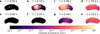 |
Fig. 2 Surface acceleration on the Kamoi (western) side (a–d) and the opposite (eastern) side (e–h) caused by seismic wave propagation at (a, e) 0 s (initial condition), (b, f) 0.1 s, (c, g) 0.4 s, and (d, h) 10 s after the impact. |
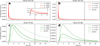 |
Fig. 3 Time-varying acceleration experienced by each facet. (a) Acceleration at facet 152 for different diffusivity values: K = 1000 m2 s−1 (Simulation 2, dotted), K = 2000 m2 s−1 (Simulation 1, solid), and K = 3000 m2 s−1 (Simulation 3, dashed). (b) Acceleration at facet 152 for different seismic efficiency values: η = 5.0 × 10⁻⁸ (Simulation 5, dotted), η = 1.0 × 10⁻⁷ (Simulation 1, solid), and η = 5.0 × 10⁻⁷ (Simulation 8, dashed). (c, d) Same as (a, b), but for facet 93. The horizontal dotted line represents the gravitational acceleration at each facet. The vertical dashed line marks t = 10 seconds, when the simulation ended and exponential decay extrapolation began. |
3 Results
In this section, we present the numerical results derived from our two-step simulation framework. Section 3.1 reports the results of the surface acceleration caused by seismic shaking, based on the diffusion model introduced in Sect. 2.1. Section 3.2 then evaluates the resulting surface displacement using the landslide toy model described in Sect. 2.2.
3.1 Surface acceleration by a seismic wave
All of our simulations show that surface acceleration varies over time as the seismic wave propagates through the asteroid.
Figure 2 visualizes the acceleration changes for the nominal condition (Simulation 1 in Table 1, η = 1.0 × 10⁻⁷ and K = 3000 m2 s−1 ) on the Kamoi (western) side (Figs. 2a–d) and the opposite (eastern) side (Figs. 2e–h). We found that the seismic energy causes high accelerations greater than 1 m s−2 near the impact site within the first 0.10 seconds (Figs. 2a, b).
At around 0.40 seconds after the impact, the seismic wave reaches the head part and the opposite (eastern) side (Figs. 2c, g). For reference, 10−5 m s−2 is a typical surface gravitational acceleration on the Itokawa surface. Even after 10.0 seconds (see Figs. 2d, h), the surface acceleration remains above this typical surface gravitational acceleration (a = 10−5 m s−2) due to residual seismic energy, despite the overall attenuation.
Figure 3 shows the dependence of surface acceleration on K and η for facets A and B (defined in Fig. 1) with facet A located near and facet B farther from the Kamoi crater. Both facets experience accelerations that are higher by one order of magnitude than the local gravitational acceleration (indicated by the horizontal dotted line). Since facet A is close to the impact site, its peak acceleration is higher than that of facet B, and it appears within 0.1 seconds after the impact. In contrast, facet B shows its peak after around 1 second under the highest diffusivity condition (K = 3000 m2 s−1, dashed lines). In addition, facet A exhibits both a higher peak acceleration and a longer duration above the gravitational threshold when K is low (dotted line) or η is high (dashed red line). Conversely, facet B shows stronger acceleration under higher K (dashed green line) and η (dotted green line), although a larger K leads to faster attenuation, which reduces the time during which the acceleration exceeds gravity.
Figure 4 shows the ratio of the maximum acceleration during the 10-second simulation and the local surface gravity for the Kamoi (western) side and the opposite (eastern) side. For both sides, the ratio exceeds 0.2 across all facets. This value was previously suggested as a threshold for boulder destabilization (Miyamoto 2014). Panels a and e in Figure 4, which correspond to higher η values, show higher seismic accelerations than panels d and h with lower η values. In Simulation 10 (η = 1.0 × 10⁻⁹), the minimum acceleration ratio reaches approximately 0.2 at the facet farthest from the Kamoi crater (Figs. 4d, h).
Compared to η, the effect of changing K is weaker. To clarify the influence of diffusivity, we compared maximum accelerations from simulations with extreme K values to the nominal case in Fig. 5. The lower K cases (panels a, c) yield smaller peak accelerations than the nominal case, while the higher K cases (panels b, d) produce greater accelerations across most surface regions, except near the Kamoi crater.
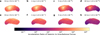 |
Fig. 4 Ratio of the maximum surface acceleration to the local gravitational acceleration on the Kamoi side (western; panels a–d) and the opposite side (eastern; panels e–h) for different η values. All simulations assume a constant K value of 2000. The panels are arranged such that η decreases from left to right. Each column corresponds to an η value of 5 × 10⁻⁷, 1 × 10⁻⁷, 5 × 10⁻⁸, and 1 × 10⁻⁹. |
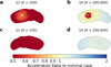 |
Fig. 5 Ratio of the maximum surface acceleration from simulations with extremely low (K = 200 m2 s−1, panels a, c) and high (K = 200 000 m2 s−1, panels b, d) diffusivity values with respect to the nominal case. Panels (a) and (b) show the Kamoi side, and panels (c) and (d) show the opposite side. |
3.2 Landslide simulation
Figure 6a shows horizontal displacements estimated using our landslide toy model. We observed that some facets exhibited large displacements even in the absence of seismic acceleration from the Kamoi impact (Fig. 6b). This is attributed to steep local slopes that exceed the angle of repose, which is 31.0° for µ = 0.6. To isolate the effect of seismic shaking, we corrected for this by subtracting the results of a control simulation without seismic input from those of the nominal simulation (Fig. 6c). Even after this correction, facets with steep slopes still showed horizontal displacements of approximately 10 mm.
The motion of boulders on facets 152 (A) and 93 (B) is shown in Fig. 7. A boulder on facet 152 is lifted from the surface by strong initial acceleration and remains at its landing position (Figs. 7a, b), as the seismic acceleration is significantly attenuated by diffusion after 2 seconds (Figs. 3a, b). Larger horizontal displacements and higher maximum heights occur under low K and high η conditions. On the other hand, in Figs. 7c and d, boulders undergo both launching and sliding by seismic shaking. The case with K = 1000 m2 s−1 (dotted green line) shows greater displacement due to the long-lasting acceleration above gravity (dotted line from Fig. 3c). No clear relation between η and displacement is found in Fig. 7d, however.
Representative simulation results using K = 1000 and 2000 m2 s−1 and η = 1 × 10⁻⁷ from Richardson et al. (2020) are shown in Fig. 8. For the Kamoi side (Figs. 8a, b), regions near the Kamoi crater, steep areas around the neck connecting the body (left) and head (right) lobes of Itokawa, and some locally steep facets exhibit horizontal displacements greater than 1 mm. On the other hand, the opposite side (Figs. 8c, d) shows lower displacements overall. Nevertheless, similar to the Kamoi side, some steep-sloped facets (particularly those near the neck) exhibit displacements on the order of 1 cm. In the case of K = 1000 m2 s−1 (Figs. 8b, d), the head lobe experiences significant horizontal motion on both sides. This trend is clearly visible in Figs. 9c and g, where the head region shows displacements that are greater by more than ten times than those in the surrounding areas. In contrast, the high-K case (Figs. 9d, h) exhibits generally low displacements, except in regions near Kamoi. The high-η case (Figs. 9a, e) shows elevated displacement values across the surface compared to the low-η case (Figs. 9b, f), except at some facets on the head lobe. In addition, Fig. 10 shows the maximum vertical height reached during the landslide on the Kamoi side. Launch heights greater than 1 mm only appear near the Kamoi crater and increase with higher η.
 |
Fig. 6 Correction process applied to the landslide simulation results. (a) Result from the simulation under the nominal case, (b) result from the simulation without seismic acceleration, and (c) difference between (a) and (b), used as the corrected displacement. |
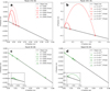 |
Fig. 7 Motion of boulders on each facet. (a) Boulder motion on facet number 152 for different diffusivity values: K = 1000 m2 s−1 (Simulation 2, dotted line with downward triangle), K = 2000 m2 s−1 (Simulation 1, solid line with square), and K = 3000 m2 s−1 (Simulation 3, dashed line with upward triangle). (b) Boulder motion on facet number 152 for different seismic efficiency values: η = 5.0 × 10⁻⁸ (Simulation 5, dotted line with downward triangle), η = 1.0 × 10⁻⁷ (Simulation 1, solid line with square), and η = 5.0 × 10⁻⁷ (Simulation 8, dashed line with upward triangle). (c) and (d) show the same comparisons as (a) and (b), respectively, but for facet 93. The markers indicate the final positions of the boulders 10 minutes after the impact. The inclined black lines represent the local surface slope. |
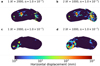 |
Fig. 8 Horizontal displacement of boulders on the western (Kamoi; panels a, b) and eastern (opposite) side (panels c, d). Panels a and c show results from Simulation 1 (η = 1.0 × 10⁻⁷, K = 2000 m2 s−1), and panels b and d show those from Simulation 2 (η = 1.0 × 10⁻⁷, K = 1000 m2 s−1), which reproduces the observed space-weathering distribution on Itokawa best. |
4 Discussion
In this section, we first examine the modeling assumptions and evaluate how they might affect the results of our seismic and landslide simulations (Sect. 4.1). We then compare the simulation outcomes with the observed distribution of space weathering on Itokawa and discuss the implications of the inferred seismic diffusivity (K) and efficiency (η) for understanding resurfacing processes on small asteroids.
4.1 Assumptions and uncertainties in seismic and landslide modeling
To make the modeling manageable, we adopted several simplifying assumptions in simulating seismic wave propagation and landslides. In the following subsections, we evaluate how these assumptions might influence our results.
4.1.1 Seismic energy propagation
We applied the Neumann boundary condition, assuming that the vacuum outside the asteroid exerts no external stress when we solved Eq. (2). This assumption neglects energy loss through launching boulders or regolith particles, a process known as the cocoa effect (Tancredi et al. 2023). These losses might slightly reduce the surface accelerations. Because this process also contributes to surface renewal, however, our conclusions are probably not compromised by omitting it, and it might also contribute to resurfacing.
We modeled the asteroid surface as a simple harmonic oscillator with a single frequency of 10 Hz. This value was chosen based on the dominant spectral peak around 10–20 Hz reported by Richardson et al. (2020). This frequency is also consistent with impact-generated seismic waves observed on the Moon (Latham et al. 1973; Duennebier & Sutton 1974). Although 10 Hz likely represents the dominant frequency generated by the Kamoi impact, real seismic waves typically contain a broad frequency spectrum.
To test the robustness of this assumption, we performed additional simulations at 1 Hz and 100 Hz. Higher-frequency simulations result in faster energy attenuation because the attenuation term in Eq. (2) is larger, which leads to surface accelerations that are lower by a factor of about two for the 100 Hz case. Despite this, the near-crater peak accelerations remained similar across all frequencies. Moreover, the overall horizontal displacement varied by less than an order of magnitude for all cases, and the locations of significantly altered terrain remained unchanged. These results suggest that the model predictions of the surface modification are relatively insensitive to the assumed frequency. This reinforces the robustness of our conclusions.
Additionally, Quillen et al. (2019) estimated the corner frequency (fc), that is, the cutoff above which the seismic source spectrum rapidly weakens, using the relation
 (6)
(6)
where the P-wave velocity υp is 100 m s−1, and the crater diameter Dcrater is 8 m (Yasui et al. 2015; Hirata et al. 2009). This yields a corner frequency of 12.5 Hz and suggests that significantly higher frequencies contribute little to the seismic response. This further supports our assumption of 10 Hz.
Furthermore, we fixed the quality factor (Q) in Eq. (2) to 1500. We adopted this value because the Q values estimated by Richardson et al. (2020) for asteroids Eros, Steins, and Itokawa range from 1500 to 2000, although their sizes are significantly different from each other. To evaluate the sensitivity of Q on the final result, we also ran simulations with Q = 500 and 4000, and we confirmed that the distribution and amount of horizontal displacements varied by less than an order of magnitude. In addition, since the attenuation term in Eq. (2) (2πf ϵ/Q) includes the frequency and Q, the effects of the frequency and Q can partially cancel out. Our model already showed robust results over a wide frequency range (1–100 Hz), and the variation in Q is therefore unlikely to affect the conclusions significantly.
Moreover, we modeled the propagation of seismic waves as a diffusion process and not as coherent wave propagation, following Richardson et al. (2005). According to Nakamura (1977), seismic waves may be treated as particles traveling through a scattering medium if the condition
 (7)
(7)
is satisfied, where D is the characteristic size of scatterers, k is a constant (typically k ≥ 1), and λ is the wavelength.
In our nominal case (K = 2000 m2 s−1 ), assuming a wave velocity of 100 m s−1 derived from impact experiments on highly porous materials (Yasui et al. 2015), we determined the mean free path l of the wave to be 60 m from Eq. (3), which may be considered as D. On the other hand, λ was derived to be 10 m from the assumed velocity and frequency. This yields k = 6, which satisfies the condition for the diffusion approximation. Therefore, it is safe to say that this is a self-consistent simulation to simplify seismic wave propagation using the diffusion equation given by Eq. (2).
Although our simulation results indicate that Itokawa has lower seismic diffusivity values (K) than other asteroids (Richardson et al. 2020), which reflects its highly scattering interior nature, our model does not explicitly account for wave reflections and scattering at interfaces between interior blocks within Itokawa. This simplification might either lead to an over-estimation or underestimation of the seismic energy transport. A more advanced approach, such as the smooth-sphere discrete element method, might capture these complexities better and might be explored in future studies.
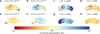 |
Fig. 9 Horizontal displacement ratio relative to the nominal case (Simulation 1). Panels a–d show the Kamoi (western) side, and panels e–h show the opposite (eastern) side. The first two columns present simulation results with η values of 5.0 × 10⁻⁸ (a, e) and 5.0 × 10⁻⁷ (b, f). The last two columns show simulation results with K values of 1000 m2 s−1 (c, g) and 3000 m2 s−1 (d, h). |
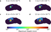 |
Fig. 10 Maximum vertical displacement of boulders during the simulation on the Kamoi (western) side. Panels (a–d) correspond to η values of 5 × 10⁻⁸, 1 × 10⁻⁷, 5 × 10⁻⁷, and 1 × 10⁻⁶. In panels (a–c), the maximum displacement ranges from 1 cm to 1 m, whereas in panel (d), it exceeds 1 m. |
4.1.2 Landslide toy model
We used a low-resolution shape model to eliminate the effects of boulder-scale topography in the original shape model (Gaskell 2020). This simplification might overlook small-scale landslides on steep local slopes, particularly those that are smaller than a few tens of meters in scale. As a result, our model cannot reproduce localized landslides, such as those that occur at crater rims or along ridge flanks. We acknowledge this limitation and revisit it in Sect. 4.2.
Additionally, we assumed that acceleration only acts along the surface normal, which might neglect lateral shaking effects. The simple harmonic oscillator assumption might also become less accurate when the mass of a boulder is comparable to the local substrate volume. In these cases, the boulder and underlying surface behave as a coupled mass system and not as a driven oscillator, which reduces the relative acceleration and displacement. This effect is expected to be minor, however, because only six boulders larger than 20 m have been identified on Itokawa (Michikami et al. 2008).
We adopted a constant coefficient of friction, µ = 0.6, for the static and kinetic friction following DellaGiustina et al. (2024). To assess the sensitivity of our results, we also tested a case with a higher friction coefficient of µ = 1.0. In this case, the angle of repose increased from 31° to 45°, which reduced the number of facets that experienced sliding. Nevertheless, the overall distribution of horizontal displacements remained similar to the nominal case, which suggests that our results are robust with respect to variations in the friction coefficient.
Finally, we ignored the rolling and bouncing of boulders by assuming perfectly inelastic impacts upon landing. This may lead to an underestimation of the final horizontal travel distance. However, dark boulder surfaces even at apparently fresh terrains (Fig. 6b of Ishiguro et al. 2007) imply long surface exposure ages and launch heights of less than 1 m. This suggests that secondary motion is limited on Itokawa.
Despite the simplifications described in this subsection (i.e., the use of a low-resolution shape model, the neglect of lateral shaking and secondary motions, and the assumption of purely inelastic boulder impacts), our simulations successfully reproduce the major patterns of global seismic shaking and landslides observed on both the western and eastern hemispheres. These assumptions generally tend to underestimate the extent of landslides. Therefore, our argument that the Kamoi impact triggered global surface renewal is likely robust. The reproduction of key observational features under such limiting conditions supports the validity of our approach and strengthens our overall conclusions.
4.2 Comparison to space-weathering distribution of Itokawa
Based on observed spatial variations in space weathering, we summarize the key observational features as follows:
The Kamoi (western) side exhibits lower space-weathering degrees than the opposite (eastern) side (Ishiguro et al. 2007).
Fresh, high-albedo patches are observed around large boulders near the Kamoi crater and in the head region, likely indicating recently exposed surface material (Figs. 11b, d).
Relatively fresh terrains are also appear in localized regions on the opposite hemisphere, particularly around the southern neck and the rim of the Komaba crater (Figs. 11a: A, C; b: D).
The smooth terrain Muses Sea tends to show intermediate space-weathering degrees (Fig. 11a: F).
In the following subsections, we compare these observed features with the results of our seismic shaking simulations and discuss possible interpretations.
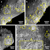 |
Fig. 11 High-resolution images of Itokawa taken by Hayabusa/AMICA. (a) Eastern (opposite) side of Itokawa (image ID: ST_2487335302). This image includes the Komaba crater with a bright rim (A), fresh surfaces on steep slopes along the Yatsugatake ridge (B), Shirakami (C), and other fresh patches near large boulders or craters (D, E). The large smooth terrain, Muses Sea, is also shown (F). (b) Western (Kamoi) side (image ID: ST_2486649845). Locations of panels (c) and (d) are marked with orange and green dashed lines, respectively. Notable features include the Kamoi crater (A), fresh surfaces near the Kamoi crater (B, C) and in the neck region (D), the mature smooth terrain Sagamihara Planitia (E), and another smooth area near the Tsukuba boulder (F). (c) Head region (image ID: ST_2483892216), showing relatively fresh terrain near a black boulder (A). (d) Close-up near the Kamoi crater (image ID: ST_2566571276), showing the crater (A), fresh basins around weathered boulders (B), and boulders with very fresh surfaces likely fractured by impact or thermal fatigue (C, D). |
4.2.1 space-weathering dichotomy between Kamoi and opposite sides
In this subsection, we assess whether our simulation results reproduce the first key observational feature: (1) the western (Kamoi) side (Fig. 11b) exhibits lower space-weathering degrees thanthe opposite side(Fig. 11a). Our simulation shows that maximum accelerations are systematically higher on the Kamoi side (e.g., Figs. 2a–d) than on the opposite side (Figs. 2e–h). As a result, surface materials on the Kamoi side experience larger horizontal displacements, increasing the likelihood that fresh subsurface materials are exposed over a broad region, not only near the impact site (Figs. 8a, b). This trend agrees with the observational evidence reported by Ishiguro et al. (2007), who reported that the Kamoi side is less weathered overall.
Hayabusa/AMICA observations also revealed terrains with intermediate space-weathering degrees. Our simulation indicate that these areas correspond to horizontal displacements of less than approximately 1 m. We propose that the intermediate space-weathering signatures result from spatial and spectral mixing between fresh and matured surfaces, causing these terrains to appear only partially weathered in remote-sensing data.
This hemispherical dichotomy also appears inconsistent with the hypothesis that thermal fatigue is the dominant resurfacing mechanism on Itokawa. Although we identified features that may have originated from boulders recently broken by thermal fatigue (Fig. 11d: C, D), these occurrences are rare. The spin axis of Itokawa is oriented at (λ, β) = (128.5°, 89.66°) (Demura et al. 2006), nearly perpendicular to its orbital plane. This orientation results in similar diurnal heating and cooling cycles across both hemispheres, which makes it difficult to explain the observed dichotomy in space-weathering degrees through thermal fatigue alone (Delbo et al. 2014).
4.2.2 Fresh surface exposures around large boulders
Close-up images (Figs. 11b: B, C; d: B) reveal bright high-albedo patches that appear to be immediately adjacent to large boulders in some boulder-rich regions, particularly near the Kamoi crater and the head part. These features are interpreted as exposures of the original substrate where the boulders were once seated, which became freshly exposed by seismic shaking. The elevated reflectance of these patches suggests that the subsurface material was less weathered, and the motion of boulders helped uncover these fresh surfaces. Most of these bright patches on the western (Kamoi) side are reproduced in our simulations (Figs. 8a, b). For example, around the Kamoi crater, including its upper left (Fig. 11b: C) and lower (Fig. 11b: B) portions, leading to boulders that are displaced and redeposited atop others, thereby exposing the previously buried substrate.
We estimate that a minimum launching height of approximately 1 cm, comparable to the characteristic grain size of Itokawa, is sufficient to expose fresh material (Miyamoto et al. 2007). We also infer, however, that the maximum launching height does not exceed about 1 meter because most boulders retain high space-weathering degrees, suggesting that they were not significantly overturned. Based on this constraint, we narrow the plausible range of seismic efficiency η to between 5.0 × 10⁻⁸ and 5.0 × 10⁻⁷, as shown in Fig. 10. This range is consistent with the estimates of Richardson et al. (2020) for Itokawa.
4.2.3 Localized fresh terrains on the opposite hemisphere
Even on the hemisphere opposite to the Kamoi side (eastern side), we observe small regions where fresh subsurface material appears to have been exposed, likely by landslides. In particular, relatively bright terrains have been identified in high-slope areas such as the southern neck region (Fig. 11b: D) and along the rim of the Komaba crater (Fig. 11a: A).
Our simulation does not reproduce these localized landslides on steep slopes, mainly because we use a simplified shape model with a reduced spatial resolution. Even with a higher-resolution model, it would be challenging to capture landslides in such small-scale steep terrains. Nevertheless, if the slopes around the crater rim were inclined at approximately 30°, our model suggests that they might become unstable under the seismic conditions we modeled. We therefore conjecture that the bright terrains observed near the Komaba crater rim and the southern neck might also have resulted from seismic shaking caused by the Kamoi impact.
Simulations with lower K values produce significant displacements in the head region that are driven by prolonged accelerations that exceed the gravitational threshold (see Fig. 3). These displacements correspond well with observed fresh terrains (Fig. 11c: A), suggesting that K likely falls within the range of 1000–2000 m2 s−1. This K estimate is consistent with that of Richardson et al. (2020).
In summary, our results support the hypothesis that the Kamoi impact induced global seismic shaking that triggered landslides even on the opposite hemisphere. They also explain the distribution of fresh terrains on both sides of Itokawa.
4.2.4 Moderate space-weathering degrees in the Muses Sea
Smooth terrains on Itokawa, such as Muses Sea (Fig. 11a: F), tend to exhibit moderate degrees of space weathering. Prelanding images revealed that these areas are covered with finegrained regolith composed of millimeter- to centimeter-sized particles (Yano et al. 2006). These fine particles are susceptible to granular convection, a process that stirs the regolith vertically and horizontally and redistributes materials from different depths (Miyamoto et al. 2007). As a result, the continuous mixing of mature and relatively fresh particles may lead to an intermediate spectral signature that appears as moderately weathered terrain in remote-sensing data.
This interpretation is also consistent with the laboratory analyses of Itokawa samples, which were mostly collected from the Muses Sea region. These sampled particles exhibit space-weathered rims on the examined grains (Matsumoto et al. 2015), suggesting that regolith mixing through granular convection allowed even subsurface particles to be exposed and weathered over time. We thus infer that the observed moderate space-weathering degrees are a result of long-term regolith turnover that extends to depths of a few meters and leads to a spatially averaged weathering state across the smooth terrains (Yano et al. 2006).
In summary, our simulation results are broadly consistent with the observed space-weathering patterns on Itokawa. All key features can be explained by seismic shaking and landslides triggered by the Kamoi impact. Only small-scale features remain unresolved by the resolution of the shape model, but the overall spatial trends are reproduced well.
4.3 Unique space-weathering properties of Itokawa among S-type asteroids
Itokawa is unique among S-type near-Earth asteroids visited by spacecraft, such as (433) Eros, (4179) Toutatis, and (65803) Didymos, as fresh surface exposures are widespread across its surface. In addition, other S-type asteroids in the main belt, (951) Gaspra and (243) Ida, exhibit globally weathered matured surfaces. We consider the origin of the unusual surface freshness of Itokawa below.
Figure 4 shows that the maximum surface acceleration exceeded the conventional threshold for boulder destabilization (0.2; Miyamoto 2014) across the entire surface by an order of magnitude at least. Even in the conservative Simulation 10, which assumed only 1% of the seismic energy of the nominal case, the minimum acceleration-to-gravity ratio still reached 0.2 (Figs. 4d, h). This result suggests that even impacts smaller than the Kamoi event might have triggered global seismic shaking and surface renewal.
Assuming constant seismic efficiency, density, and impact velocity, we estimate that the minimum impactor mass required to induce global seismic shaking on Itokawa is as small as 4.3 g (Figs. 4d, h). According to the standard interplanetary dust flux model (Grün et al. 1985), collisions like this are expected to occur approximately once every 20 000 years for an asteroid of the size of Itokawa. Based on the estimated space-weathering timescale of ~1000 years for S-type asteroids, we infer that more than 5% of sub-kilometer-sized asteroids might statistically exhibit fresh surfaces as a result of a single impact (Jin & Ishiguro 2022). This probability is non-negligible. Therefore, it is reasonable to expect that future missions will encounter additional small asteroids with surface characteristics similar to those of Itokawa.
We note, however, that some previous studies have suggested a much longer space-weathering timescale of up to 107 years. If this were the case, even small impacts that occurred every ~104 years would suffice to refresh surfaces over geological timescales, and widespread fresh terrains would be common among S-type near-Earth asteroids. These features are rare except for Itokawa, however. This discrepancy may support the notion that space weathering proceeds rapidly, in ~103 years, which is consistent with our results and sample-based estimates (Nagao 2011; Noguchi et al. 2014; Jin & Ishiguro 2022).
These findings not only explain the exceptional surface freshness of Itokawa, but also underscore the potential of a space-weathering analysis as a diagnostic tool for investigating the surface and internal properties of asteroids. Our method can be extended to other mission-targeted asteroids, such as Dimorphos, the secondary of (65803) Didymos, which was targeted by the Double Asteroid Redirection Test (DART) mission. The kinetic energy of the DART impactor was approximately 2.8 times greater than that of the Kamoi impactor, and the Dimorphos diameter (~ 150 m) is about half that of Itokawa (Graykowski et al. 2023). These characteristics suggest that the DART impact may have triggered global seismic shaking on Dimorphos, which might have led to surface disturbances that would be observable by the Hera mission.
Moreover, future missions such as the extended Hayabusa2 mission to (98943) Torifune and the exploration of Origins, Spectral Interpretation, Resource Identification and Security – Apophis Explorer (OSIRIS-APEX) of (99942) Apophis might benefit from applying our approach, particularly if fresh craters similar to Kamoi are found. Expanding this analysis to multiple rubble-pile bodies will deepen our understanding of the internal diversity and evolutionary paths of small asteroids.
4.4 Seismic diffusivity (K) and the rubble-pile structure of Itokawa
We estimated the seismic diffusivity (K) of Itokawa to be in the range of 1000-2000 m2 s−1. This value was derived from the geographic distribution of landslide features reproduced in our simulations, as shown in Fig. 8. The K value for Itokawa is only about 2% of those estimated for (433) Eros (~ 17 km) and (2867) Steins (~5 km) (Richardson et al. 2020), which suggests that the interior structure of Itokawa is more strongly dominated by scattering than these larger S-type asteroids. This difference is likely attributable to its smaller size and higher porosity.
Assuming a seismic wave velocity of 100 m s−1, based on the impact experiments of Yasui et al. (2015), we estimate the corresponding mean free path to be 30–60 m. This implies that the interior of Itokawa likely hosts many tens-of-meter-sized blocks, comparable to the largest surface boulder, Yoshinodai (~50 × 30 × 20 m). This mean free path is significantly shorter than the overall dimensions of Itokawa (535×294×209 m), indicating that seismic waves are strongly scattered at tens-of-meters scales. Itokawa was the first asteroid that was confirmed to have a rubble-pile structure based on two lines of definitive evidence: the abundance of surface boulders, and the high porosity of ~40% (Fujiwara et al. 2006). The internal distribution and size of the subsurface boulders remain poorly understood, however.
Our seismic modeling suggests that the interior is filled with numerous boulders that are an order of magnitude smaller than the body size. For a porosity of 40%, the number of these blocks may range between 104 and 105. Therefore, our study provides unique dynamical evidence based on seismic wave propagation modeling that supports the hypothesis that the Itokawa interior is truly a rubble pile.
We also estimated the seismic efficiency (η) for Itokawa to range from 5.0 × 10⁻⁸ to 5.0 × 10⁻⁷. This is lower by an order of magnitude than the values reported for Eros and Steins (Richardson et al. 2020), and it is significantly lower than the values for the Moon and Mars (Latham et al. 1970; Lognonné et al. 2020). We interpret this low efficiency as a consequence of the high porosity of Itokawa and the armoring effect of its boulder-rich surface. Laboratory experiments using unarmored sand targets have yielded higher efficiencies on the order of 10−5 (Yasui et al. 2015; Matsue et al. 2020), which further supports our interpretation of the low η value for Itokawa.
5 Summary
We simulated impact-induced seismic shaking and subsequent landslides on asteroid Itokawa to assess the influence of the Kamoi impact on the surface space weathering. Our results show that an impactor as small as 4.3 g can induce surface accelerations that are sufficient to destabilize boulders across the entire surface. The simulations revealed that fresh material that was originally buried beneath boulders can be exposed through ejecta launch or downslope motion. These findings are consistent with spatial variations in space weathering observed by the Hayabusa spacecraft.
By reproducing the observed surface patterns, we constrained the seismic diffusivity to 1000–2000 m2 s−1, suggesting the presence of interior blocks on the order of 10 meters. We also estimated the seismic efficiency to be on the order of 10−7. The agreement between our estimates and previous studies supports the hypothesis that space-weathering distributions can be used as diagnostic tools for inferring the surface and internal physical properties of asteroids.
Acknowledgements
This research was supported by a National Research Foundation of Korea (NRF) grant funded by the Korean government (MEST) (No. 2023R1A2C1006180). SJ was supported by the Research Scholarship for Ph.D. studies from the National Research Foundation of Korea (NRF) grant funded by the Korean Government (RS-2024-00407585).
References
- Ballouz, R. L., Agrusa, H., Barnouin, O. S., et al. 2024, Planet. Sci. J., 5, 251 [Google Scholar]
- Bonal, L., Quirico, E., Bourot-Denise, M., & Montagnac, G. 2015, Meteor. Planet. Sci., 50, 1562 [NASA ADS] [CrossRef] [Google Scholar]
- Chapman, C. R. 2004, Annu. Rev. Earth Planet. Sci., 32, 539 [CrossRef] [Google Scholar]
- Clark, B. E., Hapke, B., Pieters, C., & Britt, D. 2002, in Asteroids III, eds. W. F. Bottke, Jr., A. Cellino, P. Paolicchi, & R. P. Binzel (University of Arizona Press), 585 [Google Scholar]
- Dainty, A. M., Toksöz, M. N., Anderson, K. R., et al. 1974, Moon, 9, 11 [Google Scholar]
- Delbo, M., Libourel, G., Wilkerson, J., et al. 2014, Nature, 508, 233 [Google Scholar]
- DellaGiustina, D. N., Ballouz, R. L., Walsh, K. J., et al. 2024, MNRAS, 528, 6568 [Google Scholar]
- Demura, H., Kobayashi, S., Nemoto, E., et al. 2006, Science, 312, 1347 [NASA ADS] [CrossRef] [Google Scholar]
- Duennebier, F., & Sutton, G. H. 1974, J. Geophys. Res., 79, 4365 [Google Scholar]
- Ernst, C. M., Barnouin, O. S., Daly, R. T., & Small Body Mapping Tool Team 2018, in 49th Annual Lunar and Planetary Science Conference, Lunar and Planetary Science Conference, 1043 [Google Scholar]
- Fujiwara, A., Kawaguchi, J., Yeomans, D. K., et al. 2006, Science, 312, 1330 [NASA ADS] [CrossRef] [Google Scholar]
- Garland, M., & Heckbert, P. S. 1997, in Proceedings of SIGGRAPH '97 (ACM Press), 209 [Google Scholar]
- Gaskell, R. W. 2020, Gaskell Phobos Shape Model V1.0, NASA Planetary Data System, urn:nasa:pds:gaskell.phobos.shape-model::1.0 [Google Scholar]
- Graykowski, A., Lambert, R. A., Marchis, F., et al. 2023, Nature, 616, 461 [NASA ADS] [CrossRef] [Google Scholar]
- Grün, E., Zook, H. A., Fechtig, H., & Giese, R. H. 1985, Icarus, 62, 244 [NASA ADS] [CrossRef] [Google Scholar]
- Hapke, B. 2001, J. Geophys. Res., 106, 10039 [NASA ADS] [CrossRef] [Google Scholar]
- Hirata, N., Barnouin-Jha, O. S., Honda, C., et al. 2009, Icarus, 200, 486 [NASA ADS] [CrossRef] [Google Scholar]
- Ishiguro, M., Hiroi, T., Tholen, D. J., et al. 2007, Meteor. Planet. Sci., 42, 1791 [NASA ADS] [CrossRef] [Google Scholar]
- Jin, S., & Ishiguro, M. 2022, A&A, 667, A93 [NASA ADS] [CrossRef] [EDP Sciences] [Google Scholar]
- Kanamaru, M., Sasaki, S., & Wieczorek, M. 2019, Planet. Space Sci., 174, 32 [CrossRef] [Google Scholar]
- Keller, L. P., & Berger, E. L. 2014, Earth Planets Space, 66, 71 [NASA ADS] [CrossRef] [Google Scholar]
- Koga, Y., Noguchi, T., Nakamura, T., et al. 2018, Icarus, 299, 386 [CrossRef] [Google Scholar]
- Latham, G., Ewing, M., Dorman, J., et al. 1970, Science, 170, 620 [Google Scholar]
- Latham, G., Ewing, M., Dorman, J., et al. 1973, Moon, 7, 396 [Google Scholar]
- Lognonné, P., Banerdt, W. B., Pike, W. T., et al. 2020, Nat. Geosci., 13, 213 [CrossRef] [Google Scholar]
- Lowry, S. C., Weissman, P. R., Duddy, S. R., et al. 2014, A&A, 562, A48 [NASA ADS] [CrossRef] [EDP Sciences] [Google Scholar]
- Matsue, K., Yasui, M., Arakawa, M., & Hasegawa, S. 2020, Icarus, 338, 113520 [Google Scholar]
- Matsumoto, T., Tsuchiyama, A., Miyake, A., et al. 2015, Icarus, 257, 230 [CrossRef] [Google Scholar]
- Matsumoto, T., Hasegawa, S., Nakao, S., Sakai, M., & Yurimoto, H. 2018, Icarus, 303, 22 [NASA ADS] [CrossRef] [Google Scholar]
- Michikami, T., Nakamura, A. M., Hirata, N., et al. 2008, Earth Planets Space, 60, 13 [NASA ADS] [Google Scholar]
- Miyamoto, H. 2014, Planet. Space Sci., 95, 94 [NASA ADS] [CrossRef] [Google Scholar]
- Miyamoto, H., Yano, H., Scheeres, D. J., et al. 2007, Science, 316, 1011 [CrossRef] [Google Scholar]
- Nagao, K. e. a. 2011, Science, 333, 1128 [NASA ADS] [CrossRef] [Google Scholar]
- Nakamura, Y. 1977, J. Geophys. Z. Geophys., 43, 389 [Google Scholar]
- Noguchi, T. e. a. 2011, Science, 333, 1121 [NASA ADS] [CrossRef] [Google Scholar]
- Noguchi, T., Kimura, M., Hashimoto, T., et al. 2014, Meteor. Planet. Sci., 49, 188 [CrossRef] [Google Scholar]
- Pieters, C. M., & Noble, S. K. 2016, J. Geophys. Res. (Planets), 121, 1865 [NASA ADS] [CrossRef] [Google Scholar]
- Pieters, C. M., Taylor, L. A., Noble, S. K., et al. 2000, Meteor. Planet. Sci., 35, 1101 [NASA ADS] [CrossRef] [Google Scholar]
- Quillen, A. C., Zhao, Y., Chen, Y., et al. 2019, Icarus, 319, 312 [Google Scholar]
- Richardson, J. E., Melosh, H. J., Greenberg, R. J., & O’Brien, D. P. 2005, Icarus, 179, 325 [NASA ADS] [CrossRef] [Google Scholar]
- Richardson, J. E., Steckloff, J. K., & Minton, D. A. 2020, Icarus, 347, 113811 [NASA ADS] [CrossRef] [Google Scholar]
- Saito, J., Miyamoto, H., Nakamura, R., et al. 2006, Science, 312, 1341 [NASA ADS] [CrossRef] [Google Scholar]
- Sasaki, S., Nakamura, K., Hamabe, Y., Kurahashi, E., & Hiroi, T. 2001, Nature, 410, 555 [NASA ADS] [CrossRef] [Google Scholar]
- Tancredi, G., Liu, P.-Y., Campo-Bagatin, A., Moreno, F., & Domínguez, B. 2023, MNRAS, 522, 2403 [Google Scholar]
- Tatsumi, E., & Sugita, S. 2018, Icarus, 300, 227 [NASA ADS] [CrossRef] [Google Scholar]
- Virtanen, P., Gommers, R., Oliphant, T. E., et al. 2020, Nat. Methods, 17, 261 [Google Scholar]
- Yano, H., Kubota, T., Miyamoto, H., et al. 2006, Science, 312, 1350 [NASA ADS] [CrossRef] [Google Scholar]
- Yasui, M., Matsumoto, E., & Arakawa, M. 2015, Icarus, 260, 320 [Google Scholar]
All Tables
All Figures
|
Fig. 1 Three-dimensional views of (a) the original shape model of Itokawa with 49 152 facets from Gaskell (2020) and (b) the simplified model with 1024 facets used in this study. The blue star denotes the location of the Kamoi crater. Red (A) and green (B) facets correspond to facets 152 and 93, respectively, and are used for comparison in Figs. 3 and 7. |
| In the text | |
|
Fig. 2 Surface acceleration on the Kamoi (western) side (a–d) and the opposite (eastern) side (e–h) caused by seismic wave propagation at (a, e) 0 s (initial condition), (b, f) 0.1 s, (c, g) 0.4 s, and (d, h) 10 s after the impact. |
| In the text | |
|
Fig. 3 Time-varying acceleration experienced by each facet. (a) Acceleration at facet 152 for different diffusivity values: K = 1000 m2 s−1 (Simulation 2, dotted), K = 2000 m2 s−1 (Simulation 1, solid), and K = 3000 m2 s−1 (Simulation 3, dashed). (b) Acceleration at facet 152 for different seismic efficiency values: η = 5.0 × 10⁻⁸ (Simulation 5, dotted), η = 1.0 × 10⁻⁷ (Simulation 1, solid), and η = 5.0 × 10⁻⁷ (Simulation 8, dashed). (c, d) Same as (a, b), but for facet 93. The horizontal dotted line represents the gravitational acceleration at each facet. The vertical dashed line marks t = 10 seconds, when the simulation ended and exponential decay extrapolation began. |
| In the text | |
|
Fig. 4 Ratio of the maximum surface acceleration to the local gravitational acceleration on the Kamoi side (western; panels a–d) and the opposite side (eastern; panels e–h) for different η values. All simulations assume a constant K value of 2000. The panels are arranged such that η decreases from left to right. Each column corresponds to an η value of 5 × 10⁻⁷, 1 × 10⁻⁷, 5 × 10⁻⁸, and 1 × 10⁻⁹. |
| In the text | |
|
Fig. 5 Ratio of the maximum surface acceleration from simulations with extremely low (K = 200 m2 s−1, panels a, c) and high (K = 200 000 m2 s−1, panels b, d) diffusivity values with respect to the nominal case. Panels (a) and (b) show the Kamoi side, and panels (c) and (d) show the opposite side. |
| In the text | |
|
Fig. 6 Correction process applied to the landslide simulation results. (a) Result from the simulation under the nominal case, (b) result from the simulation without seismic acceleration, and (c) difference between (a) and (b), used as the corrected displacement. |
| In the text | |
|
Fig. 7 Motion of boulders on each facet. (a) Boulder motion on facet number 152 for different diffusivity values: K = 1000 m2 s−1 (Simulation 2, dotted line with downward triangle), K = 2000 m2 s−1 (Simulation 1, solid line with square), and K = 3000 m2 s−1 (Simulation 3, dashed line with upward triangle). (b) Boulder motion on facet number 152 for different seismic efficiency values: η = 5.0 × 10⁻⁸ (Simulation 5, dotted line with downward triangle), η = 1.0 × 10⁻⁷ (Simulation 1, solid line with square), and η = 5.0 × 10⁻⁷ (Simulation 8, dashed line with upward triangle). (c) and (d) show the same comparisons as (a) and (b), respectively, but for facet 93. The markers indicate the final positions of the boulders 10 minutes after the impact. The inclined black lines represent the local surface slope. |
| In the text | |
|
Fig. 8 Horizontal displacement of boulders on the western (Kamoi; panels a, b) and eastern (opposite) side (panels c, d). Panels a and c show results from Simulation 1 (η = 1.0 × 10⁻⁷, K = 2000 m2 s−1), and panels b and d show those from Simulation 2 (η = 1.0 × 10⁻⁷, K = 1000 m2 s−1), which reproduces the observed space-weathering distribution on Itokawa best. |
| In the text | |
|
Fig. 9 Horizontal displacement ratio relative to the nominal case (Simulation 1). Panels a–d show the Kamoi (western) side, and panels e–h show the opposite (eastern) side. The first two columns present simulation results with η values of 5.0 × 10⁻⁸ (a, e) and 5.0 × 10⁻⁷ (b, f). The last two columns show simulation results with K values of 1000 m2 s−1 (c, g) and 3000 m2 s−1 (d, h). |
| In the text | |
|
Fig. 10 Maximum vertical displacement of boulders during the simulation on the Kamoi (western) side. Panels (a–d) correspond to η values of 5 × 10⁻⁸, 1 × 10⁻⁷, 5 × 10⁻⁷, and 1 × 10⁻⁶. In panels (a–c), the maximum displacement ranges from 1 cm to 1 m, whereas in panel (d), it exceeds 1 m. |
| In the text | |
|
Fig. 11 High-resolution images of Itokawa taken by Hayabusa/AMICA. (a) Eastern (opposite) side of Itokawa (image ID: ST_2487335302). This image includes the Komaba crater with a bright rim (A), fresh surfaces on steep slopes along the Yatsugatake ridge (B), Shirakami (C), and other fresh patches near large boulders or craters (D, E). The large smooth terrain, Muses Sea, is also shown (F). (b) Western (Kamoi) side (image ID: ST_2486649845). Locations of panels (c) and (d) are marked with orange and green dashed lines, respectively. Notable features include the Kamoi crater (A), fresh surfaces near the Kamoi crater (B, C) and in the neck region (D), the mature smooth terrain Sagamihara Planitia (E), and another smooth area near the Tsukuba boulder (F). (c) Head region (image ID: ST_2483892216), showing relatively fresh terrain near a black boulder (A). (d) Close-up near the Kamoi crater (image ID: ST_2566571276), showing the crater (A), fresh basins around weathered boulders (B), and boulders with very fresh surfaces likely fractured by impact or thermal fatigue (C, D). |
| In the text | |
Current usage metrics show cumulative count of Article Views (full-text article views including HTML views, PDF and ePub downloads, according to the available data) and Abstracts Views on Vision4Press platform.
Data correspond to usage on the plateform after 2015. The current usage metrics is available 48-96 hours after online publication and is updated daily on week days.
Initial download of the metrics may take a while.