| Issue |
A&A
Volume 703, November 2025
|
|
|---|---|---|
| Article Number | A69 | |
| Number of page(s) | 20 | |
| Section | Planets, planetary systems, and small bodies | |
| DOI | https://doi.org/10.1051/0004-6361/202556176 | |
| Published online | 07 November 2025 | |
The Pedersen and Hall conductances in the Jovian polar regions: New maps based on a broadband electron energy distribution
1
Laboratory for Planetary and Atmospheric Physics, University of Liège,
Liège,
Belgium
2
Aix-Marseille Université, CNRS, CNES, Institut Origines, LAM,
Marseille,
France
3
Institute of Geophysics and Meteorology, University of Cologne,
Cologne,
Germany
4
Institute for Space Astrophysics and Planetology, National Institute for Astrophysics (INAF-IAPS),
Rome,
Italy
5
Southwest Research Institute,
San Antonio,
TX,
USA
6
Physics and Astronomy Department, University of Texas at San Antonio,
TX,
USA
7
Univ. Grenoble Alpes, CNRS, IPAG,
38000
Grenoble,
France
★ Corresponding author: This email address is being protected from spambots. You need JavaScript enabled to view it.
Received:
30
June
2025
Accepted:
5
September
2025
Abstract
Context. The ionospheric Pedersen and Hall conductances play an important role in understanding the coupling by which angular momentum, energy, and matter are exchanged between the magnetosphere, ionosphere and thermosphere at Jupiter, modifying the composition and temperature of the planet. In the high-latitude regions, the Pedersen and Hall conductances are enhanced by the auroral electron precipitation.
Aims. We investigated the effect of a broadband-precipitating electron energy distribution, similar to the observed electron distributions through particle measurements, on the Pedersen and Hall conductance values. The new conductance values were compared to those obtained from previous studies, notably for a mono-energetic distribution.
Methods. The broadband-precipitating electron energy distribution was modeled by a kappa distribution, which is used as an input in an electron transport model that computes the vertical density profiles of ionospheric ions. Assuming that the conductivity is mostly governed by the density of H3+ and CH5+, we then evaluated the vertical profiles of the Pedersen and Hall conductivities from the vertical profiles of the ion density. Finally, the Pedersen and Hall conductances were computed by integrating the corresponding conductivities over altitude.
Results. The Pedersen and Hall conductance values are globally higher for a broadband electron energy distribution instead of a mono-energetic distribution. In addition, the considered electron collision cross sections and the chosen method for computing the ion production rates can also have significant impacts on the conductance values. The comparison between our results and those deduced from corotation enforcement theory suggests that either a physical mechanism limits the field-aligned currents or the auroral electrons precipitating in the atmosphere are accelerated by processes that are not associated with the field-aligned currents.
Key words: publications, bibliography / planets and satellites: atmospheres / planets and satellites: aurorae / planets and satellites: gaseous planets
© The Authors 2025
 Open Access article, published by EDP Sciences, under the terms of the Creative Commons Attribution License (https://creativecommons.org/licenses/by/4.0), which permits unrestricted use, distribution, and reproduction in any medium, provided the original work is properly cited.
This article is published in open access under the Subscribe to Open model. This email address is being protected from spambots. You need JavaScript enabled to view it. to support open access publication.
1 Introduction
Jupiter is the largest planet in the Solar System. It is also known to host the most intense polar aurorae at its poles; they are observed at many wavelengths. They mainly result from collisions between precipitating energetic electrons with the atmospheric constituents in the upper atmosphere of the planet, H and H2. The electron precipitation also considerably enhances the ionization of the neutral species, which feeds the Jovian ionosphere and strengthens its ability to carry electric currents. The intensity of these electric current components flowing perpendicular to the magnetic field is proportional to the Pedersen and Hall conductances.
The Pedersen conductance affects the transfer of angular momentum by the large-scale field-aligned current (FAC; currents flowing along the magnetic field lines) loops that circulate between the middle magnetosphere and the high-latitude ionosphere (e.g., Hill 1979; Nichols & Cowley 2004; Smith & Aylward 2009; Tao et al. 2009). The loops are closed by radially outward-flowing currents in the magnetospheric plasma sheet and by equatorward-flowing currents in the ionosphere. In the frame of corotation enforcement theory, these currents transfer momentum from the ionosphere to the magnetosphere through a J × B torque that maintains part of the constant outwardflowing magnetospheric plasma in corotation with the Jovian magnetic field (Hill 1979) up to a radial distance that varies between 20 RJ and 40 RJ (1RJ = 71 492 km), depending on local time. In this framework, the Pedersen conductance affects the transfer of angular momentum and notably modulates the current intensity and the maximum distance at which the plasma corotates (Nichols & Cowley 2003, 2004). The Pedersen and Hall conductances also play a role in the transport of the magnetospheric plasma itself at radial distances <20 RJ. Notably, the interchange instabilities and plasma convection are highly dependent on the values and spatial distribution of the conductances (Wang et al. 2023). In addition, the Pedersen and Hall conductances affect the interaction between Alfvén waves, which propagate along the magnetic field lines, and the ionospheric conductive layer, in which the conductances become significant.
This interaction is depicted in the numerical model developed by Lysak et al. (2023), which describes the propagation of Alfvén wings between Io and Jupiter. This model notably shows that a higher Pedersen conductance leads to a stronger reflection of the Alfvén waves in the ionosphere. Thus, the Jovian ionospheric Pedersen and Hall conductances are key parameters for understanding the coupling between the magnetosphere and the ionosphere, that is, the exchanges of momentum, energy, and matter between the two media.
Numerous studies have attempted to constrain these values. Millward et al. (2002) used mono-energetic electron beams to study the variation of the Pedersen and Hall conductances with the mean electron energy, the electron number flux, and energy flux. They notably used the Jovian Ionospheric Model (JIM; Achilleos et al. 1998) to infer the ion density in the Jovian ionosphere. They found that the two conductances are maximum for a mean electron energy value of about 60 keV. Based on these results, Nichols & Cowley (2004) modeled the precipitating electron energy distribution as a function of the FAC density in the ionosphere and investigated the impact of this precipitation on the Pedersen conductance and its resulting positive feedback on the FAC. To understand the angular momentum transfer from the thermosphere to the magnetosphere, Smith & Aylward (2009) attempted to refine the effective Pedersen conductance by taking into account the difference of velocities (i.e., slippage) between the thermosphere and the deep interior of Jupiter due to collisions with the charged particles (Nichols & Cowley 2004). Tao et al. (2009) also computed the Pedersen conductance in a attempt to evaluate the effect of neutral winds on the magnetosphere-ionosphere-thermosphere (MIT) coupling. The variation in the conductance caused by the diurnal change in the solar extreme-ultraviolet (EUV) flux was also investigated in order to evaluate its effect on the FAC. Results from Tao et al. (2010) suggested that the Pedersen conductance varies by about 0.1 mho between the night- and the dayside.
Hiraki & Tao (2008) built an analytical expression that reproduced the vertical profile of the ionization rate that results from the energy degradation in the atmosphere of the precipitating electrons computed with Monte Carlo techniques. The availability of this analytical formulation allows us to simplify the calculations of the ionospheric ion densities and hence the conductance. The authors notably computed Pedersen conductance values assuming an H2 atmosphere and a uniform surface magnetic field of B = 8.4 × 10⁻⁴ T. In their 3D Jupiter Thermospheric General Circulation Model (JTGCM), Bougher et al. (2005) used an electron energy distribution consisting of three kappa functions to compute the ion density in the ionosphere. They found conductance values of about 10 mho, which differs from previous studies. According to the authors, the difference might arise because the H3+ vertical profile peak is generated at a deeper altitude in the JTGCM model than in the JIM model.
The above studies provided a wide range of ionospheric conductance values that did not easily match each other. According to Gérard et al. (2020), the lack of observational constraints led the authors to postulate values for important parameters that have a major influence on the conductances, such as the total electron energy flux and mean energy and the general shape of the energy distribution. The advent of the Juno mission contributed to better constraints on these parameters. The presence of hydrocarbons, which control the ion density below the methane homopause, the altitude above which the methane molecular diffusion becomes dominant compared with atmospheric turbulence, was not always addressed. This was notably the case for the JIM model, which was used in some of the studies mentioned above (e.g., Millward et al. 2002; Nichols & Cowley 2004). This issue was resolved to a certain extent in more recent studies, even though the methane homopause level is still partially unconstrained (Sinclair et al. 2025).
Several aspects are poorly addressed when the conductance is studied in the auroral regions, however. Most of these studies were restricted to the main auroral emission (ME) region, while this auroral emission represents only approximately one-third of the total auroral emission. Moreover, they often considered a precipitating electron energy distribution based on inferred ionospheric FAC density (Nichols & Cowley 2004), on the assumption that up-going FACs, corresponding to down-going electrons accelerated toward the Jovian ionosphere by field-aligned potentials predicted by corotation enforcement theory, are the root cause of the auroral ME (Cowley & Bunce 2001). The data collected by Juno and the Hubble Space Telescope (HST) over the past years challenge this theory, however, and revealed growing evidence of a more intricate process at work (Bonfond et al. 2020). Among the compelling evidence is the discrepancy between theory and observations that arises in the asymmetry in the dawn and dusk brightness of the aurorae. According to corotation enforcement theory, the dawn part of the ME should be brighter than the dusk part because the magnetic field is more strongly bent back on the dawnside (Ray et al. 2014). This prediction is not supported by observations, which show the opposite trend (Bonfond et al. 2015; Groulard et al. 2024). The observations also show that not only are the electrons accelerated bidirectionally by stochastic mechanisms in addition to field-aligned potentials (Mauk et al. 2018; Sulaiman et al. 2022), but these mechanisms are the main acceleration processes at work (Salveter et al. 2022).
In their investigation of the MIT coupling parameters, Wang et al. (2021), and at a later stage, Al Saati et al. (2022), avoided part of the problem by using electron energy distributions that were directly drawn from the data acquired by the JADE and JEDI instruments on board Juno. The electron energy distributions measured by the instruments may differ from the precipitating population, however, when the acceleration region is located between the spacecraft and the planet (Gérard et al. 2019). Gérard et al. (2020) computed Pedersen conductance maps of the overall auroral region using Juno-UVS spectral images. From the auroral brightness and a methane color ratio (CR), which is the ratio of two specific UV spectral bands absorbed and unabsorbed by hydrocarbons, they retrieved the total energy flux and the mean energy of the precipitating electrons, respectively (Gustin et al. 2016). By assuming a mono-energetic precipitating electron energy distribution, they derived the ion densities in the ionosphere using the analytic expression developed by Hiraki & Tao (2008). Nevertheless, in-situ Juno observations showed that the shape of the precipitating electron energy distribution is mostly broadband (Mauk et al. 2018; Salveter et al. 2022). The choice of a realistic electron energy distribution may be relevant for the computation of the conductance, as was already shown at low energy for the aurorae on Earth (Germany et al. 1994).
With the use of Juno data, we investigated the effect of a broadband-precipitating electron energy distribution on the ionospheric Pedersen and Hall conductances. One of the added values of this work is that the same electron transport model and distribution model were applied to retrieve the ionospheric ion densities and the precipitating mean electron energy. We describe the instruments and data in Section 2. The method we applied is described in Section 3. In Section 4, we identify the generic differences between the conductances computed with a broadband and a mono-energetic distribution and compare the conductance values for a few Juno perijoves (PJs) to already existing values. Finally, we present our conclusions in Section 5.
2 Instruments
This study is based on data collected by two instruments on board the solar-powered Juno spinning spacecraft (Bolton et al. 2017). Launched in August 2011 for a 5-year journey, Juno was inserted in orbit around Jupiter on 5 July 2016. It follows an elliptical polar orbit, which allows it to avoid most of the radiation belt regions, and it performs close flybys of Jupiter. The orbital period of Juno around the planet was initially of 53.5 days, but it was gradually reduced since the start of the extended mission campaign (PJ34+) to a value of about 32 days for the most recent PJs. The spacecraft spins at a rate of 30 seconds.
2.1 Juno-JEDI
The Jupiter Energetic-Particles Detector (JEDI) (Mauk et al. 2017a) is a set of three sensors that measure the flux of ions (H+, He+, O+, and S+) and electrons that cross the path of Juno as a function of their energy. JEDI detects electrons in the energy range 25-1000 keV. The JEDI sensor geometry allows us to instantaneously collect the electrons for almost any pitch angle, which is the angle between the electron velocity and the local magnetic field.
2.2 Juno-UVS
The Ultraviolet Imager/Spectrograph (UVS) instrument (Gladstone et al. 2014) collects EUV and far ultraviolet (FUV) photons in the 68-210 nm range, which covers part of the Lyman and Werner bands of the H2 spectrum and the Lyman-α line of H. When entering the instrument, the UV light passes through an aperture that is oriented along the spacecraft spin axis, which defines the instrument field of view (FOV). It is made up of three rectangular slits, two external wide slits and a central narrow slit in the form of a dog bone. When projected onto the sky, the two wide slits have an FOV of 2.55° × 0.2°. The narrow slit has an FOV of 2° × 0.025° and an increased spectral resolution. After the slits, a grating scatters the UV light onto the detector. A scan mirror is placed at the entrance of the spectrograph, which permits the shifting of the FOV by ±30° away from the Juno spin plane. Close to Jupiter, UVS acquires spectra with a high spatial resolution of the auroral UV emission in the polar regions.
3 Method
The ionospheric electric conductance is essentially dependent on the vertical density profiles of the different ions in the ionosphere. The main goal of this study was to assess the effect of a more realistic precipitating electron energy distribution on the Pedersen and Hall conductances, and we therefore only considered ions generated by the auroral electron precipitation. Photoionization of the atmospheric components by solar EUV radiation was neglected. This effect indeed increases the Pedersen and Hall conductances by about 0.01 mho (Tao et al. 2010; Clément et al. 2025), which is lower by 10 to 100 times than the conductance values computed in the auroral regions. We did not take ions produced by meteoric impacts into account either. Nevertheless, for a sufficient meteoric influx, this process is expected to have a non-negligible effect at Jupiter and in particular, to increase the Hall conductance (Nakamura et al. 2022; Clément et al. 2025).
In Fig. 1, we present the general flow of the method. The UVS and JEDI data were used to extract the key parameters for modeling the broadband-precipitating electron energy distribution. After setting an auroral atmosphere (see Section 3.2), we input this distribution in an electron transport model to obtain the vertical profiles of the ion density, from which we deduced the conductivities and conductances.
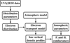 |
Fig. 1 Schematic representation of the different steps we implemented to compute the Pedersen (P) and Hall (H) conductances. The distribution parameters are the mean electron energy, the total electron energy flux, and a third parameter that is related to the high-energy slope of the broadband electron energy distribution. The ionospheric parameters include the ionospheric magnetic field intensity as well as the ion and electron collision frequencies with the neutrals. |
3.1 Precipitating auroral electron energy distribution
As mentioned in the introduction, the use of the electron energy distribution measured by JEDI might affect the computation of the conductances because in some cases, Juno flew above the region in which the precipitating electrons were accelerated. We instead chose to represent the broadband energy spectrum of the precipitating auroral electron population with a kappa distribution model (Livadiotis 2017). Its two main parameters, the mean electron energy and total electron energy flux, were deduced from the chosen CR (see equation (3)) and the auroral brightness, respectively, which do not depend on the altitude of the spacecraft.
At low energy, the kappa distribution is similar to a Maxwellian distribution. The kappa distribution has the advantage of reproducing the power-law decrease that is observed at high energy in the JEDI data (Mauk et al. 2017b), which characterizes collisionless plasma that is out of thermal equilibrium. A kappa distribution was used to study the particle environment around several celestial bodies. Coumans et al. (2002) employed it to model the proton population generating part of the FUV aurorae at Earth. The energy spectra of electrons that cause the diffuse aurorae at Earth and Ganymede were also modeled with a kappa distribution (Singhal et al. 2016; Tripathi et al. 2017, 2023). At Saturn, the effect of the electron precipitation on the ionosphere was investigated using a kappa distribution (Galand et al. 2011). At Jupiter, the energies of the electron population were modeled by a kappa distribution to investigate the heating of the Jovian atmosphere caused by the electron precipitation (Grodent et al. 2001), the Io footprint (Bonfond et al. 2009), and the ME vertical emission profile (Bonfond et al. 2015).
We used the expression of the kappa distribution from Coumans et al. (2002) to express the electron number flux,
 (1)
(1)
Here, E is the electron energy, 〈E〉 is the mean electron energy, and Fe is the total electron energy flux. The units of F(E) are s−1 m−2 sr−1 keV−1. The additional parameter κ controls the high-energy slope. The above function F(E) can also be expressed in terms of the characteristic energy Eo of the distribution. We preferred to use the mean electron energy 〈E〉, however, which is more meaningful when comparing different distributions (Robinson et al. 1987). The relation of the mean and characteristic energies is given by
 (2)
(2)
3.1.1 Retrieving Fe and 〈E〉
When Juno is at the shortest distance from Jupiter, UVS scans the Jovian aurorae once for each rotation of the spacecraft. The resulting image from each spin only covers a part of the aurorae. We used complete coverages of the northern and southern aurorae that were obtained by averaging the spectral brightness over a stack of 100 spins (Bonfond et al. 2017). The total electron energy flux Fe was derived from the total H2 auroral UV brightness, which was obtained by integrating the spectral brightness, measured by UVS, in the wavelength range 145-165 nm and then scaled by a factor of 4.4 in order to obtain the total equivalent H2 Lyman and Werner bands UV brightness (Bonfond et al. 2017). Previous studies found that a total brightness of 10 kR roughly corresponds to Fe = 1 mW.m−2 (Gérard & Singh 1982; Waite et al. 1983; Grodent et al. 2001; Nichols & Cowley 2022).
The mean electron energy 〈E〉 was retrieved from the CR deduced from UVS observations and computed as
 (3)
(3)
where I(λ) is the spectral brightness (Gérard et al. 2019). The numerator and the denominator represent parts of the UV spectrum that is not absorbed and that is absorbed by methane, respectively. This CR is different from the CR used for spectral images from the Space Telescope Imaging Spectrograph (STIS) on board HST, for which the absorbed part of the spectrum in the denominator starts at 123 nm instead of 125 nm (e.g., Gustin et al. (2016). The spectral range was adapted to account for the degradation of the UVS detector sensitivity around the Lyman-α line (about 121.6 nm), especially for the wide slits (Hue et al. 2019). The minimum value of this CR, which is the value without any absorption, is 1.8 (Benmahi et al. 2024a).
We used the CR-〈E〉 relation presented by Benmahi et al. (2024a) that was updated by Benmahi et al. (2024b). This relation is based on a UV emission model of H2 coupled to the TransPlanet electron transport model (Lilensten et al. 1989; Benmahi 2022). The authors developed a phenomenological law assuming a kappa or a mono-energetic distribution for the auroral precipitating electron energy, which gives the CR as a function of the characteristic energy E0 of the distribution and the emission angle θ, which is the angle between the local vertical and the line of sight of Juno,
![Mathematical equation: \begin{align} CR\Big(&E_0,\theta\Big) = \\ & A \, C \, \left[ \tanh \left(\frac{E_0 - E_{c}}{B}\right) + 1 \right] \, \ln^{\,\beta}\left( \left( \frac{E_0}{D} \right)^{\alpha} + e \right) \, \left[ 1 + \delta \, \sin^{\gamma}(\theta) \right]. \end{align}](/articles/aa/full_html/2025/11/aa56176-25/aa56176-25-eq4.png)
Here, A is the minimum amplitude of the CR, Ec is a threshold energy, and B, C, D, α, and β are the fit parameters. For a fixed emission angle, the characteristic energy was retrieved from the CR with the dichotomy method, a root-finding method. The mean electron energy was then deduced from the characteristic energy depending on the chosen distribution. For a mono-energetic distribution, the relation is simply 〈E〉 = E0. For the kappa distribution, the link is given by equation (2) and depends on the value of the κ parameter. We recall that as mentioned by Gustin et al. (2016), the CR-〈E〉 relation is highly dependent on the temperature profile, the CH4 methane homopause altitude, and the electron energy distribution.
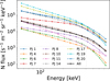 |
Fig. 2 Broadband energy distributions of electrons measured in the loss cone by JEDI for several PJs when Juno was magnetically connected to the ME region, down to a radial distance of 1.2-2.5 RJ. The number flux (N flux) values are the median values over a PJ. |
3.1.2 Retrieving κ
A Markov chain Monte Carlo method was applied to 11 sets of median JEDI electron energy distribution measurements, magnetically linked to the ME crossing, to sample the κ parameter. The JEDI data, plotted in Fig. 2, were part of the dataset used by Salveter et al. (2022). For this dataset, the distance of Juno from the center of the planet was in the range 1.2-2.5 RJ. This short radial distance ensures that the spacecraft is mostly below the acceleration region, which is expected to extend between 1.5 and 2.5 RJ (Gérard et al. 2019). The JEDI data were corrected from the minimum ionizing bump that is usually seen around 150 keV and corresponds to an excess of energy left in the detector by high-energy (>800 keV) electrons that fully penetrate the instrument (Mauk et al. 2018). A value of κ = 2.5 was retrieved, which maximizes the likelihood with a computed uncertainty of δκ = 0.48. It is worth noting that this κ value may change when auroral regions other than the ME region are considered. This possibility will be addressed in a future study.
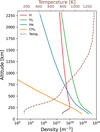 |
Fig. 3 Density and temperature profiles of the neutral atmosphere. This atmosphere is deduced from the model presented by Grodent et al. (2001). |
3.2 Vertical profile of the ion density
We now briefly describe the main steps and assumptions we applied to obtain the ion densities in the Jovian atmosphere. A complete description of the computations is provided in Appendix A. As explained in the beginning of Section 3, we only considered ions generated by collisions of auroral precipitating electrons with the principal Jovian atmospheric constituents, which were assumed to be atomic hydrogen (H), dihydrogen (H2), helium (He), and methane (CH4). Their densities were taken from the atmosphere model of Grodent et al. (2001) and are plotted in Fig. 3. The zero-reference altitude was defined as the altitude corresponding to the 1-bar pressure level.
We considered the system at steady state. The contribution of H+ to the conductance was assumed to be small because this ion is dominant above 2000 km (Tao et al. 2011), which is far above the conductive layer. The He+ ions were also neglected because their relative abundance is low (Hiraki & Tao 2008). Below the altitude region in which H+ is important and above the methane homopause, the dominant ion was then assumed to be H3+(Millward et al. 2002). Its production and loss are described by
 (4)
(4)
 (5)
(5)
Close to and below the homopause, H3+ reacts with CH4 to produce hydrocarbon ions, which become the main contributors to the conductance at these altitudes. According to Perry et al. (1999), the main hydrocarbon ions are CH5+ and C3Hn+-class ions. The production and loss of CH5+ is given by
 (6)
(6)
 (7)
(7)
The C3Hn+ ions result from a chain of ion-molecule reactions of the C and C2 hydrocarbon molecules. As in Wang et al. (2021) and Clément et al. (2025), we decided to limit our study to the CH5+ ions. This simplification allowed us to analytically solve the reaction equations in order to obtain the ion densities. The C3Hn+ ion layer is located deeper in the atmosphere, and this assumption therefore mainly affects the conductance generated by higher-energy electrons because they penetrate deeper into the atmosphere.
3.3 Electron transport model: TransPlanet
The H2+ production rate from which the H3+ ion density was derived was retrieved using the one-dimensional TransPlanet multi-stream electron transport model (Lilensten et al. 1989; Benmahi 2022).
TransPlanet is designed to compute the degradation of energy of the auroral electrons precipitating in the Jovian atmosphere. In practice, after setting an initial electron energy distribution, the model computes the evolution of the energy distribution of the auroral electrons as they travel deeper into the atmosphere and interact with their surroundings through various elastic and inelastic collisions. The energy exchanged between the electrons and the neutral atmospheric constituents is assessed by solving the dissipative Boltzmann radiative transfer equation, detailed by Benmahi (2022). The values of the semirelativistic cross sections relative to the accounted elastic and inelastic collisions between the auroral particles and the atmosphere come from the Atomic and Molecular Cross section for Ionization and Aurora Database (ATMOCIAD) (Gronoff et al. 2025).
In this study, the initial precipitating electron energy distribution input in TransPlanet was either broadband or mono-energetic. Lower- and upper-energy cutoffs were applied in the case of an initial broadband energy distribution. Electrons with a kinetic energy lower than 1 eV were considered as thermalized and hence irrelevant. In addition, we assumed that the fluxes and collision cross sections of the electrons with a kinetic energy higher than 106 eV were too small to efficiently produce conductances. Therefore, these energetic electrons were set to 0.
3.4 Conductivity and conductance
The Pedersen and Hall conductivities are defined as
 (8)
(8)
 (9)
(9)
Here, e is the electron charge, νen (νin) is the electron (ion)-neutral collision frequency, me (mi) is the electron (ion) mass, ωe (ωi) is the electron (ion) gyrofrequency, and B is the magnetic field intensity. For the conductance maps, the value of the local Jovian ionospheric magnetic field was obtained from the most recent JRM33 internal magnetic field model (Connerney et al. 2022; Wilson et al. 2023). Here, the electron and ion gyrofrequencies are defined as  and
and  .
.
The electron-neutral and ion-neutral collision frequencies are given by
 (10)
(10)
 (11)
(11)
where nn [cm−3] and α0 [10−24 cm3] are the number density and the polarizability of the considered neutral, μin is the reduced mass between the considered ion and neutral, and Te [K] is the electron temperature (Banks & Kockarts 1973; Schunk & Nagy 2009). We considered H2 as the dominant neutral species (α0,H2 = 0.82). Typically, the interactions between the suprathermal auroral electrons with the thermalized ionospheric electrons contribute to increase the electron temperature, which results in a difference between the electron and neutral temperatures. The results from a thermosphere-ionosphere model applied at Saturn (Galand et al. 2011) showed, however, that at low altitude, the neutral density is sufficiently high to effectively cool the electrons and maintain the electron temperature equal to the neutral temperature. By transposing these results to Jupiter, we found that this assumption is valid up to 800 km, which is above the altitude range of the conductive layer.
The Pedersen and Hall conductances are the corresponding conductivity integrated over the altitude
 (12)
(12)
 (13)
(13)
Since the production rate q is directly proportional to the total energy flux Fe (see Appendix A), the conductances increase as the square root of the total electron energy flux
![Mathematical equation: \Sigma_{P,H} \propto \left[\ce{H3+}\right] \propto \sqrt{q} \propto \sqrt{F_e}.](/articles/aa/full_html/2025/11/aa56176-25/aa56176-25-eq17.png) (14)
(14)
The slippage of the thermosphere is not included in those definitions. As we ultimately used conductance ratios to investigate the variations resulting from different energy distributions and because this effect is independent of the chosen precipitating electron energy distribution, we did not include it in the conductances presented in this study. Nevertheless, effective Pedersen conductance values, which take the slippage of the thermosphere into account, were computed at the end of Section 4 to compare our results to previous works.
3.5 Maps
For each PJ, the physical quantities we used (e.g., the CR, the total auroral UV brightness of H2, and the Pedersen and Hall conductances) were organized in the form of longitude-latitude maps, spanning from 0° to 360° in longitude and from −90° to 90° in latitude with an interval of 0.1° (≈100 km). For convenience, the maps we present are polar-projected. For the north pole, the projection represents the view an observer would have from above the pole. For the south pole, the maps are built to represent the view an observer would have through the planet from above the north pole. The 0° longitude in System-III is set on top of the map, and the longitude increases clockwise. As an illustration, the map of the total UV brightness of H2 for PJ1 is plotted in Fig. 4a.
For a given auroral feature, most of the emission was assumed to come from the emission peak altitude. Because Juno is not always right above the auroral emission, this peak altitude is needed to infer the location of the aurora on Jupiter. The peak altitude depends on the type of auroral emission. For example, most of the emission from the ME region is assumed to take place between 200 km and 400 km (Vasavada et al. 1999; Bonfond et al. 2015; Benmahi et al. 2024b). The Io footprint emission rather peaks at a higher altitude instead, at about 900 km (Bonfond et al. 2009). We assumed the peak emission altitude to be at 400 km above the 1-bar pressure level. As explained by Head et al. (2024), this assumption introduces an error that might shift the actual position of the aurorae up to about 100 km, depending on the position of Juno with respect to the aurorae. This error is comparable to the map resolution.
We also focused on the ME region alone. To retrieve information from this region alone, we applied masks on the polar maps that hid the auroral regions equatorward and poleward of the ME (Groulard et al. 2024). As an illustration, we applied a mask on the total UV brightness map of PJ1 north and plot the result in Fig. 4b.
Concerning the CR maps, the value on each pixel is the mean CR computed in a circle of 500 km. To avoid a low signal-to-noise ratio, the CR was only computed with the spectral brightness from the UVS wide slits and for a total auroral H2 UV brightness higher than 2 kR (Bonfond et al. 2017).
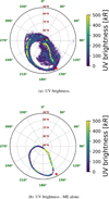 |
Fig. 4 (a) UV brightness map for PJ1 north. (b) UV brightness map for PJ1 north after we applied a mask that hides the regions poleward and equatorward of the ME. On each map, the red star represents the subsolar longitude. |
4 Results and discussion
In this section, we compare the Pedersen and Hall conductivities and conductances computed using a kappa and a mono-energetic precipitating electron energy distribution. In addition, we present and discuss the conductance maps for several Juno PJs. Hereafter, the conductivity/conductance computed using a kappa (mono-energetic) distribution is called the kappa (mono-energetic) conductivity/conductance.
4.1 Vertical conductivity profiles
Following the method described in Section 3, we computed generic vertical density profiles of H3+ and CH5+ and of the Pedersen and Hall conductivity profiles using either a kappa or a mono-energetic precipitating electron energy distribution for 〈E〉 = 10, 30, 100, and 500 keV. We assumed a total electron energy flux of 1 mW.m−2. While this value is associated with a dim aurora, the conductances ΣP,H can easily be scaled to another energy flux Fe because ΣP,H ∝ √Fe (see Section 3). We also assumed a constant magnetic field intensity of 10−3 T.
In the case of a mono-energetic distribution with a specific mean energy and total energy flux, all the electrons have a kinetic energy equal to the mean energy of the distribution, but in the case of a kappa distribution with the same mean energy and total energy flux, the electron energies are distributed between 1 eV and 1 MeV. This difference affects the vertical density profiles of H3+ and CH5+ shown in Figs. 5a to 5d. The mono-energetic electrons deposit most of their energy in a limited range of altitudes depending on the average electron energy, which results in the observed vertical profiles of the ion density with sharp peaks. The main part of the ion production is thus confined around these peaks. For a kappa distribution with the same mean energy and total energy flux, the electrons with different kinetic energy lose most of their energy at different altitudes, which leads to the observed wider and less peaked vertical ion density profiles. In particular, the high-energy electrons always reach lower altitudes up to a minimum altitude that is set by the chosen high-energy cutoff (1 MeV; see Section 3). In addition, the vertical ion density profiles computed with a kappa distribution depend less strongly on the mean energy.
The vertical Pedersen and Hall conductivity profiles are displayed in Figs. 5e-5l for the electron energy distributions and for the same set of mean energies as for the ion density profiles. For the kappa Pedersen conductivity profiles, we distinguish upper and lower conductivity peaks at about 180 km and 350 km, respectively, for all mean energy values we considered. In the case of the mono-energetic Pedersen conductivity profiles, no sharp peak appears for 〈E〉 = 10 keV. For 〈E〉 = 30 keV, only one peak is present at about 350 km, which becomes less sharp as the mean energy increases. A second peak appears at a lower altitude for 〈E〉 = 100 keV, which becomes more prominent and moves to lower altitudes as the mean energy increases. The kappa Hall conductivity is significant between about 150 km and 380 km for all the considered mean energy values. In contrast, the mono-energetic Hall profile displays a small peak at about 380 km for 〈E〉 = 10 keV. The Hall conductivity increases and the peak moves to lower altitudes as the mean energy increases. The conductivities are likely to maximize around the altitudes at which the electron and ion gyrofrequencies match their corresponding collision frequencies with the neutrals. As mentioned in the introduction, this altitude region is often called the ionospheric conductive layer (e.g., Nakamura et al. 2022; Clément et al. 2025). To be precise, the Pedersen conductivity maximizes at about the upper and lower boundaries of the conductive layer, and the Hall conductivity maximizes inside this layer. A clear definition of the conductive layer we used can be found in Appendix B.
The difference in behavior between the kappa and mono-energetic conductivities directly arises from the vertical ion profiles. We consider the conductivity profiles computed with a mono-energetic distribution. For 〈E〉 = 10 keV, most of the ions are created above the upper boundary of the conductive layer, resulting in a poor contribution to the Pedersen and Hall conductivities. For 〈E〉 = 30 keV, the peaks of the H3+ and CH5+ profiles more or less match the altitude of the upper boundary of the conductive layer. This results in a sharp Pedersen conductivity peak at about 350 km in Fig. 5f. Here, no peak appears around the lower boundary of the conductive layer because the mean energy is too low for the electrons to reach this altitude. As the electrons penetrate deeper into the atmosphere with 〈E〉 = 100 keV, the density peak of CH5+ approaches the lower boundary of the conductive layer, resulting in a second peak of Pedersen conductivity. Finally, for 〈E〉 = 500 keV, the peak of the CH5+ density matches the lower boundary of the conductive layer, giving rise to a second, lower peak for the Pedersen conductivity. Fewer ions are produced at the upper boundary of the conductive layer, however, leading to a large difference between the two peaks. The Hall conductivity also becomes non-negligible for 〈E〉 = 30, 100, and 500 keV because a significant number of electrons can reach the altitudes of the conductive layer. Understandably, the altitude of the Hall conductivity peak follows the altitude of the CH5+ density peak. When we now consider a kappa electron energy distribution, a significant number of ions are formed from 700 km down to an altitude of about 120 km for all the considered mean energies. As a consequence, all the kappa Pedersen conductivity profiles similarly display two peaks, and all the Hall profiles are extended over the altitude range of the conductive layer. As the electrons penetrate deeper in altitude with the increased mean energy, the second, lower peak of the Pedersen conductivity becomes stronger than the first, upper peak, and the Hall conductivity profile slowly deforms itself into a peaked profile.
We then integrated the Pedersen and Hall conductivity profiles to obtain the corresponding conductances. In Fig. 6 the two graphs display the evolution of the Pedersen and Hall conductances for a kappa and a mono-energetic electron energy distribution, respectively, as a function of the mean electron energy. As in Gérard et al. (2020), the mono-energetic Pedersen conductance presents a maximum value of about 30 keV, close to the value of about 60 keV previously predicted by Millward et al. (2002). The mono-energetic Pedersen conductance values obtained in this study agree with those presented by Millward et al. (2002). Their mono-energetic Hall conductance values are lower than ours by an order of magnitude, however, probably because they did not take hydrocarbon ions into account. This resulted in a depletion of electric charges, notably electrons, inside the ionospheric conductive layer, where the Hall conductivity is likely to maximize, which in turn resulted in the low computed Hall conductance. A comparison between the evolutions of the conductance as a function of the mean electron energy computed with different vertical CH4 density profiles is made in Appendix C.
The kappa Pedersen and Hall conductances present maximum values of about 60 keV and 70 keV, respectively. The mono-energetic conductance is always lower than the kappa conductance. The conductance plots directly follow the evolution of the conductivity profiles with the mean energy Notably, the very low values of the mono-energetic conductance for 〈E〉 < 10 keV reflect the fact that most of the ions are formed above the conductive layer, and the mono-energetic Pedersen conductance peak, at about 30 keV, results from the concordance between the ion density peak altitude and the upper boundary of the conductive layer. As mentioned before for the conductivities, the kappa conductances vary less with the mean energy than the corresponding mono-energetic conductances. Thus, the polar conductance maps generated assuming a kappa electron energy distribution would appear to be more uniform than those based on a mono-energetic distribution.
Finally, we computed the Pedersen ratio RP = ΣP,k/ΣP,m and Hall ratio RH = ΣH,k/ΣH,m. These ratios are plotted in Fig. 7 as a function of the mean electron energy 〈E〉. In the considered energy range, RP, RH ≥ 1. At low energy (〈E〉 ≤ 4 keV), both ratios are very high (≥ 10) and decrease as the mean energy increases. The Pedersen ratio reaches RP ≈ 1.2 at about 〈E〉 = 30 keV before it increases to RP ≈ 2 at about 〈E〉 = 130 keV. It then again decreases toward RP = 1 with the increase in the mean energy. The Hall ratio decreases to RH = 1 at about 70 keV before it increases again. These plots show that the Pedersen and Hall conductances that are computed assuming a mono-energetic electron energy distribution are generally lower inside the 1-1000 keV energy range than the conductances computed assuming a kappa electron energy distribution that spans the same range of energies.
In the auroral regions, the conductance in the low mean electron energy zones should then be affected most by a change in the electron energy distribution. Because the difference is significant for 〈E〉 < 20 keV and for 300 keV < 〈E〉, the Hall conductance should be affected by a change in the electron energy distribution either in the low and high mean energy zones in the auroral regions.
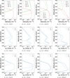 |
Fig. 5 Vertical profiles of (a)-(d) the densities of H3+ and CH5+, (e)-(h) the Pedersen conductivity and (i)-(l) the Hall conductivity, computed assuming either a kappa (K) or a mono-energetic (M) electron energy distribution and for 〈E〉 = 10, 30, 100, and 500 keV. The total electron energy flux is 1 mW.m−2. |
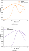 |
Fig. 6 Evolution of the (a) Pedersen and (b) Hall conductances as a function of the mean energy of the precipitating electrons 〈E〉, assuming a kappa (solid line) or a mono-energetic (dotted line) energy distribution (Fe = 1 mW.m−2, B = 10−3 T). |
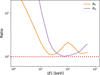 |
Fig. 7 Ratio of the kappa to mono-energetic Pedersen (RP) and Hall (RH) conductances as a function of the mean electron energy 〈E〉 (Fe = 1 mW.m−2, B = 10−3 T). |
4.2 Conductance maps
We carried out a case study by investigating the Pedersen and Hall conductances along the northern and southern polar aurorae for specific PJs. We selected PJs with a wide range of auroral characteristics. For the north pole, we chose PJ1, PJ6, PJ12, and PJ22. PJ1 and PJ6 are characterized by bright equatorward and poleward auroral emissions, respectively. The ME zones on PJ12 and PJ22 are contracted and expanded, respectively. Other features such as polar auroral filaments (Nichols et al. 2009) are also present on PJ12. For the southern hemisphere, we selected PJ15, PJ27, PJ34, and PJ35. PJ27 displays a clear auroral signature of plasma injection (Dumont et al. 2018). Finally, PJ34 and PJ35 were chosen because they display similar ME morphologies (Head et al. 2024) and subsolar longitudes.
For illustration purposes, Fig. 8 displays the Pedersen and Hall conductance maps for PJ1 built with a kappa distribution. The maps of the other PJs can be found in Appendix E. At first glance, the Pedersen and Hall conductances present similar spatial distributions for each PJ, although the Hall conductance is higher by two to three times than the Pedersen conductance. In the north, the spatial variations in the ionospheric magnetic field give rise to variations in the conductances, notably along the ME. As pointed out in Appendix B, these discrepancies are expected because the Pedersen and Hall conductances increase as the magnetic field intensity decreases. The Pedersen and Hall conductances are both larger in the ME and in the outer emission regions than in the polar emission region.
We also derived the ratio of the Pedersen (Hall) conductance maps computed with a kappa distribution to the Pedersen (Hall) conductance maps computed with a mono-energetic distribution. These ratio maps are plotted in Fig. 9 for PJ1 (see Appendix E for the maps relative to the other PJs). For the Pedersen conductance, the auroral zones that are less affected by a change in the distribution seem to be associated with a high CR (i.e., a high mean electron energy). In contrast, the local zones with strong ratio values match very low CR (i.e., low mean electron energies). The Hall ratio of part of the auroral zones is far greater than one and often matches a high CR.
For each hemisphere, the conductance maps computed with a kappa precipitating electron energy distribution display substantial spatial variations, depending on the considered auroral zones. Locally, the conductances can be about 50 mho, such as in the auroral zone that is linked to the injection event that took place during PJ27. Tables 1 and 2 show, however, that more than 95% of the kappa Pedersen and Hall conductance values remain lower than about 5 mho and 11 mho, respectively. These tables also display the median kappa conductance values computed for each PJ for the whole polar aurora, including the ME, as well as for the ME alone. The values we drew from the Pedersen conductance maps differ from those presented by Gérard et al. (2020), for which the conductance did not exceed 10 mho. In addition, our mean Pedersen conductance value computed for each PJ are higher by about three to five times than the mean conductance value obtained by Gérard et al. (2021). Here, the difference in the electron energy distribution used (kappa distribution in this study versus mono-energetic distribution in Gérard et al. (2020, 2021)) only partially explain this discrepancy. The origin of the remaining difference apparently lies within the method that is used. Gérard et al. (2020, 2021) computed the H2+ production rate using the analytical expression presented by Hiraki & Tao (2008), built from the results of an electron transport model based on a Monte Carlo simulation. In our study, the H2+ production rate is instead the direct output of the chosen electron transport model. In Appendix D we compare the mono-energetic Pedersen conductance values obtained with the analytical expression presented by Hiraki & Tao (2008) with TransPlanet and with a Monte Carlo simulation. It appears that there is a discrepancy between the use of the Hiraki & Tao (2008) analytical expression and the direct outputs of models. This discrepancy is partially but not only due to a difference in the electron collision cross sections.
The values present in Tables 1 and 2 seem to indicate that slightly more conductance is produced on average in the north than in the south when the whole polar aurora is considered. The opposite tendency is observed when the ME alone is taken into account. This latter statement might partially explain the observed difference in the mean ionospheric current density between the north and south poles (Kotsiaros et al. 2019). These asymmetries might also be linked to the already observed brightness asymmetries between the northern and southern hemispheres, for which the emissions poleward of the ME are brighter in the north and the ME is brighter in the south (Bonfond et al. 2024). As no north-south conductance asymmetry has been reported so far (Gérard et al. 2021), a statistical study of the northern and southern Pedersen and Hall conductances should be performed over the whole set of available PJs before we draw any robust conclusion.
The mean Pedersen and Hall conductance values of the ME region displayed in Tables 1 and 2 for the northern and southern aurorae globally match the ranges presented by Al Saati et al. (2022), although the mean values are slightly higher. We suggest several reasons for this discrepancy. First, the authors only had access to the conductances along the path of Juno, whereas we reach the conductances all along the ME with our method. Second, the region in which the electrons are accelerated might be below the path of Juno, as highlighted above. This acceleration would increase the auroral UV brightness, which was used to infer the total electron energy flux in our study. Finally, part of the discrepancy might be explained by the use of the analytic formula presented by Hiraki & Tao (2008) to retrieve the H2+ production rate, which was also invoked to explain the discrepancy between our results and those derived by Gérard et al. (2020).
The Pedersen conductances obtained for the ME also strongly differ from those presented by Rutala et al. (2024). By incorporating the auroral brightness observed by the HST and the magnetospheric plasma flow measured by the Galileo spacecraft in the equations relative to corotation enforcement theory, they derived median effective Pedersen conductance values relative to the ME region of  mho for the north pole and
  for the south pole. The effective conductance is related to the actual conductance through a coefficient k representing the slippage of the neutral thermosphere:
  . The observational constraints allow them to retrieve the conductance without the need to know the mass outflow rate. We took k = 0.4-0.7 (Millward et al. 2005) and computed the median effective Pedersen conductances corresponding to the actual conductance values we obtained. Without taking their error bars into account, we obtained values that were higher by 5-9 times and 6-12 times than 0.14 mho for the north and south poles, respectively. Even when we used their highest estimate, our effective conductance remained at least 1.5 times higher than theirs. In corotation enforcement theory, the effective Pedersen conductance is directly proportional to the FACs per radian of azimuth (equation 3 in Rutala et al. (2024). The effective conductance values we computed would then lead to higher FAC values that would disagree with those deduced from the Juno magnetometer measurements (Nichols & Cowley 2022). Therefore, we suggest that the discrepancy between the conductance values computed by Rutala et al. (2024) and those we computed arise from one of the following two causes or from a combination of them: Either the factor limiting the FACs is not the ionospheric conductance, but a phenomenon taking place elsewhere, or the ionospheric conductance is increased by additional precipitating electrons accelerated by processes that are not associated with the FACs. In any case, the actual relation between the FAC per radian of azimuth and the effective Pedersen conductance would then differ from the relation obtained from corotation enforcement theory.
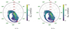 |
Fig. 8 (a) Pedersen and (b) Hall conductance maps for PJ1 north. The red star on each map represents the subsolar longitude. |
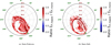 |
Fig. 9 Ratio of the Pedersen (Hall) conductance map computed with a kappa distribution over the Pedersen (Hall) conductance map computed with a mono-energetic distribution. The scale goes up to 2, but the ratio can be higher locally. The green star on each map represents the subsolar longitude. |
Pedersen conductance.
Hall conductance.
5 Conclusions
We used a kappa distribution to model the energy distribution of the auroral electrons that precipitate at the poles in the Jovian atmosphere and computed the ionospheric Pedersen and Hall conductances resulting from this precipitation. We used data from UVS and JEDI to retrieve the distribution parameters. We assumed an atmosphere made up of H, H2, He, and CH4 with densities taken from Grodent et al. (2001) and used an electron transport model (TransPlanet) to infer the vertical ion density profiles. The conductance maps were computed with the most advanced internal magnetic field model, JRM33, that is currently available for Jupiter (Connerney et al. 2022). We observed that the Pedersen and Hall conductivities are more broadly distributed in altitudes when they are computed with a kappa electron energy distribution than with a mono-energetic distribution. As a consequence, the Pedersen and Hall conductance values are higher when they are computed with a kappa electron energy distribution than with a mono-energetic distribution. This underestimation varies in strength with the mean electron energy, and it decreases when the mean energy decreases. We then computed the northern and southern conductance maps for a series of PJs and observed that the conductances are higher and more uniform on the maps associated with a kappa electron energy distribution. We also noted that the Pedersen conductance values we obtained are higher in general than those derived in previous studies. The difference is particularly large when we compare our values with those computed through corotation enforcement theory (Cowley & Bunce 2001). From these observations, we drew conclusions below:
The determination of the Pedersen and Hall conductances is significantly affected when a broadband electron energy distribution is considered instead of a mono-energetic distribution. This effect is especially strong at a low mean electron energy for the Pedersen conductance and at a low and high mean electron energy for the Hall conductance;
The high values we obtained for the Pedersen conductance are only partially due to the consideration of a more realistic precipitating electron energy distribution. The use of the analytical expression presented by Hiraki & Tao (2008) also appears to give lower conductance values than the direct outputs of electron transport models. This difference is partially but not only due to a difference in the electron collision cross sections;
The disagreement between our values and those deduced from corotation enforcement theory might indicate that either a physical mechanism that takes place elsewhere contributes to limiting the FACs and/or precipitating electrons accelerated by processes that are not associated with the FACs increase the ionospheric conductance.
Our study also highlighted the possible existence of a northsouth asymmetry in the Pedersen and Hall conductances. This asymmetry will be further investigated in a future statistical analysis of the conductance over the whole set of available PJs.
Acknowledgements
This work was supported by the Fonds de la Recherche Scientifique - FNRS under Grant(s) No. T003524F. T. Greathouse was funded by the NASA’s New Frontiers Program for Juno via contract NNM06AA75C with the Southwest Research Institute. B. Bonfond is a Research Associate of the Fonds de la Recherche Scientifique - FNRS.
Appendix A Densities of H3+ and CH5+
In the Jovian atmosphere, a fraction of the H2 molecules is ionized through collisions with the auroral precipitating electrons
 (A.1)
(A.1)
The newly formed H2+ ions rapidly react with H2 to form H3+
 (A.2)
(A.2)
The H3+ ions are essentially destroyed by dissociative recombination and reactions with methane
 (A.3)
(A.3)
 (A.4)
(A.4)
Here, αH3+ and k are the reaction rate coefficients. We take  m3 s−1 (Sundström et al. 1994) and k = 2.9 × 10⁻¹⁵ m3 s−1 (Perry et al. 1999). The quantity Te is the electron temperature that we consider equal to the neutral temperature (see main text). The equation A.4 also depicts the primary reaction that produces CH5+. These hydrocarbon ions are mainly destroyed through electron recombination
 (A.5)
(A.5)
with  m3 s−1 (Perry et al. 1999). The evolutions of the ion densities [H3+] and [CH5+] with time are governed by
![Mathematical equation: \odv{\left[\ce{H3+}\right]}{t} &= P(\ce{H3+}) - D(\ce{H3+}) + T(\ce{H3+}),](/articles/aa/full_html/2025/11/aa56176-25/aa56176-25-eq28.png) (A.6)
(A.6)
![Mathematical equation: \odv{\left[\ce{CH5+}\right]}{t} &= P(\ce{CH5+}) - D(\ce{CH5+}) + T(\ce{CH5+}).](/articles/aa/full_html/2025/11/aa56176-25/aa56176-25-eq29.png) (A.7)
(A.7)
Here, P, D and T are the production, loss and transport rates, respectively. We assumed that the atmosphere was in photochemical equilibrium, implying that the transport terms T(H3+) and T(CH5+) are equal to zero, and that the ion densities are at steady states, giving ![Mathematical equation: $\odv{\left[\ce{H3+}\right]}{t} = \odv{\left[\ce{CH5+}\right]}{t} = 0$](/articles/aa/full_html/2025/11/aa56176-25/aa56176-25-eq30.png) . The H3 + and H2+ production rates are almost equal since H2+ rapidly reacts with H2 and we write P(H3+) ≈ P(H2+) ≡ q. Typical vertical profiles of q for the two kinds of distribution considered in this study are plotted in Fig. A.1a. The equations A.6 and A.7 become
. The H3 + and H2+ production rates are almost equal since H2+ rapidly reacts with H2 and we write P(H3+) ≈ P(H2+) ≡ q. Typical vertical profiles of q for the two kinds of distribution considered in this study are plotted in Fig. A.1a. The equations A.6 and A.7 become
![Mathematical equation: 0 &= q - \alpha_{\ce{H3+}} \, \left[\ce{H3+}\right] \, \left[\ce{e-}\right] - k \, \left[\ce{H3+}\right] \, \left[\ce{CH4}\right],\\](/articles/aa/full_html/2025/11/aa56176-25/aa56176-25-eq31.png) (A.8)
(A.8)
![Mathematical equation: 0 &= k \, \left[\ce{H3+}\right] \, \left[\ce{CH4}\right] - \alpha_{\ce{CH5+}} \, \left[\ce{CH5+}\right] \, \left[\ce{e-}\right].](/articles/aa/full_html/2025/11/aa56176-25/aa56176-25-eq32.png) (A.9)
(A.9)
We assume charge equilibrium [e−] = [H3+] + [CH5+] and inject it in the above equations. We obtain a set of two equations with the two ion densities as unknowns
![Mathematical equation: 0 &= q - \alpha_{\ce{H3+}} \left[\ce{H3+}\right] \, \Big(\left[\ce{H3+}\right] + \left[\ce{CH5+}\right]\Big) - k \, \left[\ce{H3+}\right]\left[\ce{CH4}\right],](/articles/aa/full_html/2025/11/aa56176-25/aa56176-25-eq33.png) (A.10)
(A.10)
![Mathematical equation: 0 &= k \, \left[\ce{H3+}\right]\left[\ce{CH4}\right] - \alpha_{\ce{CH5+}} \left[\ce{CH5+}\right] \, \Big(\left[\ce{H3+}\right] + \left[\ce{CH5+}\right]\Big).](/articles/aa/full_html/2025/11/aa56176-25/aa56176-25-eq34.png) (A.11)
(A.11)
To analytically solve this system, we make the additional assumption that the loss rate coefficients αH3+ and αCH5+ are equal: αH3+ = αCH5+ = α. By choosing the value of αH3+ (αCH5+) for α, we shift the equilibrium towards more (fewer) ions in the atmosphere and compute an upper (lower) limit for the conductance. For a chosen mean electron energy and total energy flux, the conductance is taken as the mean value of the corresponding upper and lower boundary values. The boundary and mean values are illustrated in Fig. A.2 for the Pedersen conductance computed using a kappa electron energy distribution. Consequently, the system of equations (A.10)-(A.11) yields the following expressions for the ion densities
![Mathematical equation: \left[\ce{CH5+}\right] &= \frac{k \, \left[\ce{CH4}\right] \sqrt{\frac{q}{\alpha}}}{k \, \left[\ce{CH4}\right] + \alpha \sqrt{\frac{q}{\alpha}}}, \\](/articles/aa/full_html/2025/11/aa56176-25/aa56176-25-eq35.png) (A.12)
(A.12)
![Mathematical equation: \left[\ce{H3+}\right] &= \sqrt{\frac{q}{\alpha}} \, - \, \left[\ce{CH5+}\right].](/articles/aa/full_html/2025/11/aa56176-25/aa56176-25-eq36.png) (A.13)
(A.13)
As an illustration, the vertical density profiles of these ions are plotted in Fig. A.1b for 〈E〉 = 10 keV.
 |
Fig. A.1 (a) Production rate vertical profiles of H2+ (q) and (b) vertical density profiles of H3+ and CH5+ computed with a kappa (K) and a mono-energetic (M) electron energy distribution (〈E〉 = 10 keV, Fe = 1 mW.m−2). |
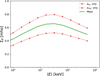 |
Fig. A.2 Pedersen conductance computed using a kappa electron energy distribution. The upper (lower) red curve represents the conductance when using the value of |


Appendix B The conductive layer
The electron and ion dynamics determine the altitudes where the Pedersen and Hall conductivities are likely to be the highest. We can highlight this dynamics in the expressions of the conductivities (8) and (9) by grouping together the ion (electron) collision frequencies with the neutrals and the ion (electron) gyrofrequencies
 (B.1)
(B.1)
 (B.2)
(B.2)
with

The vertical profiles of pe, pi, he and hi, plotted in Fig. B.1 for B = 10−3 T, set the altitudes where the Pedersen and Hall conductivities are likely to maximize. At high altitude, there are almost no collision. We have then νen = νin ≈ 0 leading to pe = Pi ≈ 0 and he = hi ≈ 1. As a result, there is almost no conductivity. As we go deeper into the atmosphere, the increase of density results in more collisions, leading to an increase of νen and νin which modify the values of pe, pi, he and hi. The vertical distributions of pe and pi present a peak value at the altitudes where νen = ωe and νin = ωi. Thus, the Pedersen conductivity is likely to maximize around these altitudes. Concerning the vertical distributions of he and hi, they drop at different altitudes. Since the electrons are much lighter than the ions, we have ωe >> ωi. As a result, he decreases at a deeper altitude than hi. Due to the presence of the minus sign in equation (B.2), the Hall conductivity is then likely to maximize in the altitude region where he ≈ 1 and hi ≈ 0 (i.e., νen << νin).
The ionosphere layer present between the altitudes where νin = ωi and νen = ωe is often called the conductive layer (Nakamura et al. 2022; Clément et al. 2025). Since we consider two kinds of ions (H3+ and CH5+), we define the altitude of the conductive layer upper boundary halfway between the altitudes where we have νCH5+ = ωCH5+ and νH3+ = ωH3+ (see Fig. B.1). The Hall and Pedersen conductivities are likely to maximize inside the conductive layer and around its boundaries, respectively.
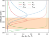 |
Fig. B.1 Vertical profiles of pe, pi, he and hi for B = 10−3 T. The orange rectangle represents the location of the conductive layer. |
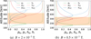 |
Fig. B.2 Effect of the magnetic field intensity on the vertical profiles of pe, pi, he and hi. The orange rectangle represents the location of the conductive layer. |
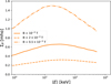 |
Fig. B.3 Evolutions of the Pedersen conductance Σp with the mean electron energy 〈E〉 for different values of the magnetic field intensity B. In addition to a change in the magnitude of Σp, the mean energy value that maximizes conductance slightly shifts toward lower (higher) values with an increase (decrease) of B. |
The conductive layer location depends on the magnetic field intensity (Nakamura et al. 2022). We illustrated the effect of a change in the magnetic field intensity on the factors pe, pi, he and hi present in the expressions (B.1) and (B.2). On Fig. B.2, we plotted their vertical profiles with different magnetic field intensity. We see that an increase (decrease) of the magnetic field intensity shifts the peaks of the vertical profiles towards lower (higher) altitudes and contributes to move down (up) the conductive layer. As a consequence, a change in the magnetic field intensity changes the evolution of the conductance with the mean electron energy, as illustrated in Fig. B.3 for the Pedersen conductance. As shown in Gérard et al. (2020), this effect has a greater impact on the conductances in the northern hemisphere due to the magnetic anomaly.
Appendix C Impact of a change in the vertical CH4 density profile
We evaluated the impact of a change in the CH4 density profile on the Pedersen and Hall conductances. In Fig. C.1a are plotted the CH4 abundance profile used in this study as well as two other profiles computed from the A and C eddy diffusion models of Moses et al. (2005) and Hue et al. (2018). The CH4 profiles mainly differ by their homopause level.
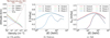 |
Fig. C.1 (a) Different vertical CH4 density profiles derived from the model of Grodent et al. (2001) (red curve) and from the A and C diffusion models of Moses et al. (2005) and Hue et al. (2018) (green and blue curves). The temperature is taken from Grodent et al. (2001). (b)-(c) Evolutions of the Pedersen and Hall conductances with the mean electron energy computed with the vertical CH4 profiles plotted in (a). |
The evolution of the Pedersen and Hall conductances, computed using either a kappa or a mono-energetic electron energy distribution, as a function of the mean electron energy, is plotted in Fig. C.1b and C.1 for the different CH4 density profiles considered. We see that the Pedersen conductance is almost insensitive to a change in the CH4 profiles. Concerning the Hall conductance, there is a difference of maximum 0.1 mho between the conductance computed with the CH4 profile from Grodent et al. (2001) and the other profiles.
Appendix D Influence of the electron transport model
The electron transport model used to determine the vertical distribution of charged particles resulting from the auroral electron precipitation, may play a role in the computation of the Pedersen and Hall conductances. In Fig. D.1 are plotted the evolutions of the mono-energetic Pedersen conductance with the mean electron energy, computed with TransPlanet, a Monte Carlo simulation and the analytical expression taken from Hiraki & Tao (2008), built on the results of a Monte Carlo simulation. For a part of the results, we also modified the ionization cross sections of H2, which are among the most significant cross sections, to see the impact on the conductance. The cross sections used in the Monte Carlo simulation were identical as the ones used to compute the results of this study with TransPlanet. We also computed the conductance values using TransPlanet in which we incorporated the ionization cross sections of H2 from Hiraki & Tao (2008). To better compare our results, the conductance values were computed assuming an atmosphere only composed of H2.
The likeliness between the red and green curves in Fig. D.1 leads to the comforting conclusion that different types of electron transport model give similar results when they use similar electron collision cross sections. In addition, the noticeable differences beyond 10 keV between the green and orange curves mean that a change in the collision cross sections, in particular the ionization cross sections of H2 , has a significant impact on the computation of the conductance. Finally, the fact that the orange and blue curves diverge seems to indicate that the analytical expression from Hiraki & Tao (2008) has to be used with caution.
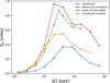 |
Fig. D.1 Evolution of the mono-energetic Pedersen conductance computed with TransPlanet (green and orange curves), a Monte Carlo simulation (red curve) and the analytical expression from Hiraki & Tao (2008) (blue curve) giving the ion production rate. The green and red curves are computed with the same ionization cross sections of H2, which are the cross sections used in this study, and the blue and orange curves are computed with the ionization cross sections from Hiraki & Tao (2008). |
Appendix E Additional maps
Here, we present the conductance maps for all the PJs considered in this study.
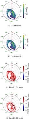 |
Fig. E.1 Conductance maps of the northern auroral region during PJ1. (a) and (b) represent the kappa Pedersen and Hall conductance maps, respectively. The ratios of the conductance map computed with a kappa electron energy distribution over the conductance map computed with a mono-energetic electron energy distribution are also represented for the (c) Pedersen and (d) Hall conductances. For the ratio maps, the scale goes up to 2 but the ratio can be locally higher. On each map, the red or green star represents the subsolar longitude. |
References
- Achilleos, N., Miller, S., Tennyson, J., et al. 1998, J. Geophys. Res.: Planets, 103, 20089 [Google Scholar]
- Al Saati, S., Clément, N., Louis, C., et al. 2022, J. Geophys. Res.: Space Phys., 127 [Google Scholar]
- Banks, P. M., & Kockarts, G. 1973, Aeronomy (New York London: Academic Press) [Google Scholar]
- Benmahi, B. 2022, PhD thesis, Université de Bordeaux [Google Scholar]
- Benmahi, B., Bonfond, B., Benne, B., et al. 2024a, A&A, 685, A26 [Google Scholar]
- Benmahi, B., Bonfond, B., Benne, B., et al. 2024b, A&A, 691, A91 [NASA ADS] [CrossRef] [EDP Sciences] [Google Scholar]
- Bolton, S. J., Lunine, J., Stevenson, D., et al. 2017, Space Sci. Rev., 213, 5 [CrossRef] [Google Scholar]
- Bonfond, B., Grodent, D., Gérard, J.-C., et al. 2009, J. Geophys. Res.: Space Phys., 114 [Google Scholar]
- Bonfond, B., Gustin, J., Gérard, J.-C., et al. 2015, Ann. Geophys., 33, 1211 [CrossRef] [Google Scholar]
- Bonfond, B., Gladstone, G. R., Grodent, D., et al. 2017, Geophys. Res. Lett., 44, 4463 [NASA ADS] [CrossRef] [Google Scholar]
- Bonfond, B., Yao, Z., & Grodent, D. 2020, J. Geophys. Res.: Space Phys., 125, e2020JA028152 [Google Scholar]
- Bonfond, B., Groulard, A., Benmahi, B., et al. 2024, in Proceedings of the Magnetospheres of the Outer Planets (MOP) 2024 Conference, Minneapolis, Minnesota, USA (F.R.S.-FNRS - Fonds de la Recherche Scientifique) [Google Scholar]
- Bougher, S. W., Waite, J. H., Majeed, T., & Gladstone, G. R. 2005, J. Geophys. Res.: Planets, 110, 2003JE002230 [Google Scholar]
- Clément, N., Nakamura, Y., Blanc, M., Wang, Y., & Al Saati, S. 2025, J. Geophys. Res.: Space Phys., 130, e2024JA033061 [Google Scholar]
- Connerney, J. E. P., Timmins, S., Oliversen, R. J., et al. 2022, J. Geophys. Res.: Planets, 127, e2021JE007055 [NASA ADS] [CrossRef] [Google Scholar]
- Coumans, V., Gérard, J.-C., & Hubert, B. 2002, J. Geophys. Res., 107, 1347 [Google Scholar]
- Cowley, S., & Bunce, E. 2001, Planet. Space Sci., 49, 1067 [Google Scholar]
- Dumont, M., Grodent, D., Radioti, A., et al. 2018, J. Geophys. Res.: Space Phys., 123, 8489 [CrossRef] [Google Scholar]
- Galand, M., Moore, L., Mueller-Wodarg, I., Mendillo, M., & Miller, S. 2011, J. Geophys. Res.: Space Phys., 116 [Google Scholar]
- Germany, G. A., Torr, D. G., Richards, P. G., Torr, M. R., & John, S. 1994, J. Geophys. Res.: Space Phys., 99, 23297 [Google Scholar]
- Gladstone, G. R., Persyn, S. C., Eterno, J. S., et al. 2014, Space Sci. Rev., 213, 447 [Google Scholar]
- Grodent, D., Waite, J. H., & Gérard, J.-C. 2001, J. Geophys. Res.: Space Phys., 106, 12933 [Google Scholar]
- Gronoff, G., Simon Wedlund, C., Hegyi, B., et al. 2025, Advances in Space Research, 75, 8232 [Google Scholar]
- Groulard, A., Bonfond, B., Grodent, D., et al. 2024, Icarus, 413, 116005 [NASA ADS] [CrossRef] [Google Scholar]
- Gustin, J., Grodent, D., Ray, L., et al. 2016, Icarus, 268, 215 [NASA ADS] [CrossRef] [Google Scholar]
- Gérard, J., & Singh, V. 1982, J. Geophys. Res.: Space Phys., 87, 4525 [CrossRef] [Google Scholar]
- Gérard, J., Bonfond, B., Mauk, B. H., et al. 2019, J. Geophys. Res.: Space Phys., 124, 8298 [Google Scholar]
- Gérard, J., Gkouvelis, L., Bonfond, B., et al. 2020, J. Geophys. Res.: Space Phys., 125, e2020JA028142 [Google Scholar]
- Gérard, J., Gkouvelis, L., Bonfond, B., et al. 2021, J. Geophys. Res.: Space Phys., 126, e2020JA028949 [Google Scholar]
- Head, L. A., Grodent, D., Bonfond, B., et al. 2024, A&A, 688, A205 [NASA ADS] [CrossRef] [EDP Sciences] [Google Scholar]
- Hill, T. 1979, J. Geophys. Res.: Space Phys., 84, 6554 [NASA ADS] [CrossRef] [Google Scholar]
- Hiraki, Y., & Tao, C. 2008, Ann. Geophys., 26, 77 [Google Scholar]
- Hue, V., Hersant, F., Cavalié, T., Dobrijevic, M., & Sinclair, J. 2018, Icarus, 307, 106 [Google Scholar]
- Hue, V., Randall Gladstone, G., Greathouse, T. K., et al. 2019, AJ, 157, 90 [NASA ADS] [CrossRef] [Google Scholar]
- Kotsiaros, S., Connerney, J. E. P., Clark, G., et al. 2019, Nat. Astron., 3, 904 [NASA ADS] [CrossRef] [Google Scholar]
- Lilensten, J., Kofman, W., Wisemberg, J., Oran, E. S., & DeVore, C. R. 1989, Ann. Geophys., 7, 83 [NASA ADS] [Google Scholar]
- Livadiotis, G. 2017, Kappa Distributions: Theory and Applications in Plasmas (Amsterdam Oxford Cambridge, MA: Elsevier) [Google Scholar]
- Lysak, R. L., Sulaiman, A. H., Bagenal, F., & Crary, F. 2023, J. Geophys. Res.: Space Phys., 128, e2022JA031180 [Google Scholar]
- Mauk, B. H., Haggerty, D. K., Jaskulek, S. E., et al. 2017a, Space Sci. Rev., 213, 289 [Google Scholar]
- Mauk, B. H., Haggerty, D. K., Paranicas, C., et al. 2017b, Geophys. Res. Lett., 44, 4410 [CrossRef] [Google Scholar]
- Mauk, B. H., Haggerty, D. K., Paranicas, C., et al. 2018, Geophys. Res. Lett., 45, 1277 [CrossRef] [Google Scholar]
- Millward, G., Miller, S., Stallard, T., Aylward, A. D., & Achilleos, N. 2002, Icarus, 160, 95 [Google Scholar]
- Millward, G., Miller, S., Stallard, T., Achilleos, N., & Aylward, A. D. 2005, Icarus, 173, 200 [Google Scholar]
- Moses, J. I., Fouchet, T., Bézard, B., et al. 2005, J. Geophys. Res.: Planets, 110, 2005JE002411 [Google Scholar]
- Nakamura, Y., Terada, K., Tao, C., et al. 2022, J. Geophys. Res.: Space Phys., 127, e2022JA030312 [Google Scholar]
- Nichols, J. D., & Cowley, S. W. H. 2003, Ann. Geophys., 21, 1419 [Google Scholar]
- Nichols, J. D., & Cowley, S. W. H. 2004, Ann. Geophys., 22, 1799 [Google Scholar]
- Nichols, J. D., & Cowley, S. W. H. 2022, J. Geophys. Res.: Space Phys., 127, e2021JA030040 [NASA ADS] [CrossRef] [Google Scholar]
- Nichols, J. D., Clarke, J. T., Gérard, J. C., & Grodent, D. 2009, Geophys. Res. Lett., 36, 2009GL037578 [Google Scholar]
- Perry, J. J., Kim, Y. H., Fox, J. L., & Porter, H. S. 1999, J. Geophys. Res.: Planets, 104, 16541 [NASA ADS] [CrossRef] [Google Scholar]
- Ray, L. C., Achilleos, N. A., Vogt, M. F., & Yates, J. N. 2014, J. Geophys. Res.: Space Phys., 119, 4740 [CrossRef] [Google Scholar]
- Robinson, R. M., Vondrak, R. R., Miller, K., Dabbs, T., & Hardy, D. 1987, J. Geophys. Res., 92, 2565 [Google Scholar]
- Rutala, M. J., Clarke, J. T., Vogt, M. F., & Nichols, J. D. 2024, J. Geophys. Res.: Space Phys., 129, e2023JA032122 [NASA ADS] [CrossRef] [Google Scholar]
- Salveter, A., Saur, J., Clark, G., & Mauk, B. H. 2022, J. Geophys. Res.: Space Phys., 127 [Google Scholar]
- Schunk, R., & Nagy, A. 2009, Ionospheres: Physics, Plasma Physics, and Chemistry, 2nd edn. (Cambridge University Press) [Google Scholar]
- Sinclair, J. A., Greathouse, T. K., Giles, R. S., et al. 2025, Planet. Sci. J., 6, 15 [Google Scholar]
- Singhal, R. P., Tripathi, A. K., Halder, S., & Ii, O. N. S. 2016, ApJ, 832, 172 [Google Scholar]
- Smith, C. G. A., & Aylward, A. D. 2009, Ann. Geophys., 27, 199 [Google Scholar]
- Sulaiman, A. H., Mauk, B. H., Szalay, J. R., et al. 2022, J. Geophys. Res.: Space Phys., 127 [Google Scholar]
- Sundström, G., Mowat, J. R., Danared, H., et al. 1994, Science, 263, 785 [Google Scholar]
- Tao, C., Fujiwara, H., & Kasaba, Y. 2009, J. Geophys. Res.: Space Phys., 114, 2008JA013966 [Google Scholar]
- Tao, C., Fujiwara, H., & Kasaba, Y. 2010, Planet. Space Sci., 58, 351 [Google Scholar]
- Tao, C., Badman, S. V., & Fujimoto, M. 2011, Icarus, 213, 581 [Google Scholar]
- Tripathi, A. K., Singhal, R. P., & Singh Ii, O. N. 2017, Ann. Geophys., 35, 239 [Google Scholar]
- Tripathi, A. K., Singhal, R. P., & Wendel, D. E. 2023, Astrophys. Space Sci., 368, 61 [Google Scholar]
- Vasavada, A. R., Bouchez, A. H., Ingersoll, A. P., Little, B., & Anger, C. D. 1999, J. Geophys. Res.: Planets, 104, 27133 [NASA ADS] [CrossRef] [Google Scholar]
- Waite, J. H., Cravens, T. E., Kozyra, J., et al. 1983, J. Geophys. Res.: Space Phys., 88, 6143 [NASA ADS] [CrossRef] [Google Scholar]
- Wang, Y., Blanc, M., Louis, C., et al. 2021, J. Geophys. Res.: Space Phys., 126 [Google Scholar]
- Wang, Y., Yang, J., Guo, X., Wang, C., & Blanc, M. 2023, J. Geophys. Res.: Space Phys., 128, e2022JA031132 [Google Scholar]
- Wilson, R. J., Vogt, M. F., Provan, G., et al. 2023, Space Sci. Rev., 219, 15 [NASA ADS] [CrossRef] [Google Scholar]
All Tables
All Figures
|
Fig. 1 Schematic representation of the different steps we implemented to compute the Pedersen (P) and Hall (H) conductances. The distribution parameters are the mean electron energy, the total electron energy flux, and a third parameter that is related to the high-energy slope of the broadband electron energy distribution. The ionospheric parameters include the ionospheric magnetic field intensity as well as the ion and electron collision frequencies with the neutrals. |
| In the text | |
|
Fig. 2 Broadband energy distributions of electrons measured in the loss cone by JEDI for several PJs when Juno was magnetically connected to the ME region, down to a radial distance of 1.2-2.5 RJ. The number flux (N flux) values are the median values over a PJ. |
| In the text | |
|
Fig. 3 Density and temperature profiles of the neutral atmosphere. This atmosphere is deduced from the model presented by Grodent et al. (2001). |
| In the text | |
|
Fig. 4 (a) UV brightness map for PJ1 north. (b) UV brightness map for PJ1 north after we applied a mask that hides the regions poleward and equatorward of the ME. On each map, the red star represents the subsolar longitude. |
| In the text | |
|
Fig. 5 Vertical profiles of (a)-(d) the densities of H3+ and CH5+, (e)-(h) the Pedersen conductivity and (i)-(l) the Hall conductivity, computed assuming either a kappa (K) or a mono-energetic (M) electron energy distribution and for 〈E〉 = 10, 30, 100, and 500 keV. The total electron energy flux is 1 mW.m−2. |
| In the text | |
|
Fig. 6 Evolution of the (a) Pedersen and (b) Hall conductances as a function of the mean energy of the precipitating electrons 〈E〉, assuming a kappa (solid line) or a mono-energetic (dotted line) energy distribution (Fe = 1 mW.m−2, B = 10−3 T). |
| In the text | |
|
Fig. 7 Ratio of the kappa to mono-energetic Pedersen (RP) and Hall (RH) conductances as a function of the mean electron energy 〈E〉 (Fe = 1 mW.m−2, B = 10−3 T). |
| In the text | |
|
Fig. 8 (a) Pedersen and (b) Hall conductance maps for PJ1 north. The red star on each map represents the subsolar longitude. |
| In the text | |
|
Fig. 9 Ratio of the Pedersen (Hall) conductance map computed with a kappa distribution over the Pedersen (Hall) conductance map computed with a mono-energetic distribution. The scale goes up to 2, but the ratio can be higher locally. The green star on each map represents the subsolar longitude. |
| In the text | |
|
Fig. A.1 (a) Production rate vertical profiles of H2+ (q) and (b) vertical density profiles of H3+ and CH5+ computed with a kappa (K) and a mono-energetic (M) electron energy distribution (〈E〉 = 10 keV, Fe = 1 mW.m−2). |
| In the text | |
|
Fig. A.2 Pedersen conductance computed using a kappa electron energy distribution. The upper (lower) red curve represents the conductance when using the value of |
| In the text | |
|
Fig. B.1 Vertical profiles of pe, pi, he and hi for B = 10−3 T. The orange rectangle represents the location of the conductive layer. |
| In the text | |
|
Fig. B.2 Effect of the magnetic field intensity on the vertical profiles of pe, pi, he and hi. The orange rectangle represents the location of the conductive layer. |
| In the text | |
|
Fig. B.3 Evolutions of the Pedersen conductance Σp with the mean electron energy 〈E〉 for different values of the magnetic field intensity B. In addition to a change in the magnitude of Σp, the mean energy value that maximizes conductance slightly shifts toward lower (higher) values with an increase (decrease) of B. |
| In the text | |
|
Fig. C.1 (a) Different vertical CH4 density profiles derived from the model of Grodent et al. (2001) (red curve) and from the A and C diffusion models of Moses et al. (2005) and Hue et al. (2018) (green and blue curves). The temperature is taken from Grodent et al. (2001). (b)-(c) Evolutions of the Pedersen and Hall conductances with the mean electron energy computed with the vertical CH4 profiles plotted in (a). |
| In the text | |
|
Fig. D.1 Evolution of the mono-energetic Pedersen conductance computed with TransPlanet (green and orange curves), a Monte Carlo simulation (red curve) and the analytical expression from Hiraki & Tao (2008) (blue curve) giving the ion production rate. The green and red curves are computed with the same ionization cross sections of H2, which are the cross sections used in this study, and the blue and orange curves are computed with the ionization cross sections from Hiraki & Tao (2008). |
| In the text | |
|
Fig. E.1 Conductance maps of the northern auroral region during PJ1. (a) and (b) represent the kappa Pedersen and Hall conductance maps, respectively. The ratios of the conductance map computed with a kappa electron energy distribution over the conductance map computed with a mono-energetic electron energy distribution are also represented for the (c) Pedersen and (d) Hall conductances. For the ratio maps, the scale goes up to 2 but the ratio can be locally higher. On each map, the red or green star represents the subsolar longitude. |
| In the text | |
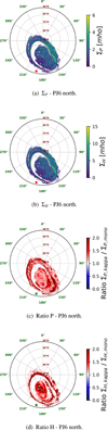 |
Fig. E.2 Same description as Fig. E.1 for PJ6 north. |
| In the text | |
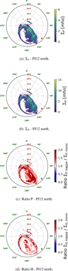 |
Fig. E.3 Same description as Fig. E.1 for PJ12 north. |
| In the text | |
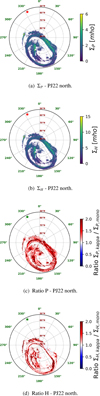 |
Fig. E.4 Same description as Fig. E.1 for PJ22 north. |
| In the text | |
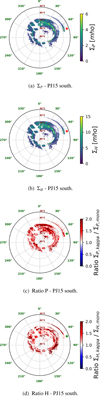 |
Fig. E.5 Same description as Fig. E.1 for PJ15 south. |
| In the text | |
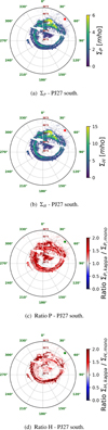 |
Fig. E.6 Same description as Fig. E.1 for PJ27 south. |
| In the text | |
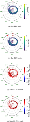 |
Fig. E.7 Same description as Fig. E.1 for PJ34 south. |
| In the text | |
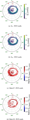 |
Fig. E.8 Same description as Fig. E.1 for PJ35 south. |
| In the text | |
Current usage metrics show cumulative count of Article Views (full-text article views including HTML views, PDF and ePub downloads, according to the available data) and Abstracts Views on Vision4Press platform.
Data correspond to usage on the plateform after 2015. The current usage metrics is available 48-96 hours after online publication and is updated daily on week days.
Initial download of the metrics may take a while.