| Issue |
A&A
Volume 703, November 2025
|
|
|---|---|---|
| Article Number | A241 | |
| Number of page(s) | 11 | |
| Section | The Sun and the Heliosphere | |
| DOI | https://doi.org/10.1051/0004-6361/202556232 | |
| Published online | 18 November 2025 | |
Role of magnetic shear distribution in the formation of eruptive flux ropes
1
Instituto de Astrofísica de Canarias, 38205 La Laguna, Tenerife, Spain
2
Universidad de La Laguna, 38206 La Laguna, Tenerife, Spain
3
Departament de Física, Universitat de les Illes Balears, E-07122 Palma de Mallorca, Spain
4
Institute of Applied Computing and Community Code (IAC3), UIB, E-07122 Palma de Mallorca, Spain
5
Indian Institute of Astrophysics, Koramangala, Bangalore 560034, India
6
Center for Space Plasma and Aeronomic Research, The University of Alabama in Huntsville, Huntsville, AL 35899, USA
7
School of Engineering, Physics, and Mathematics, Northumbria University, Newcastle upon Tyne NE1 8ST, UK
⋆ Corresponding author: This email address is being protected from spambots. You need JavaScript enabled to view it.
; This email address is being protected from spambots. You need JavaScript enabled to view it.
Received:
3
July
2025
Accepted:
12
September
2025
Abstract
Context. Erupting flux ropes play a crucial role in powering a wide range of solar transients, including flares, jets, and coronal mass ejections. These events are driven by the release of stored magnetic energy, facilitated by the shear in complex magnetic topologies. However, the mechanisms governing the formation and eruption of flux ropes, particularly the role of magnetic shear distribution in coronal arcades, are not fully understood.
Aims. We investigate how the spatial distribution of magnetic shear along coronal arcades influences the formation and evolution of eruptive flux ropes, with a focus on the evolution of mean shear during different phases of the eruption process.
Methods. We employed 2.5D resistive magnetohydrodynamic (MHD) simulations incorporating nonadiabatic effects of optically thin radiative losses, magnetic field-aligned thermal conduction, and spatially varying background heating in order to realistically model the coronal environment. A stratified solar atmosphere under gravity was initialized with a non-force-free field comprising sheared arcades. We studied two different cases by varying the initial shear to analyze their resulting dynamics and the possibility of flux rope formation and eruptions.
Results. Our results show that strong initial magnetic shear leads to spontaneous flux rope formation and eruption via magnetic reconnection, driven by the Lorentz force. The persistence and distribution of shear along the arcades are crucial in determining the formation and onset of flux rope instabilities. The shear distribution infers the non-potentiality distributed along arcades and demonstrates its relevance in identifying sites prone to eruptive activity. We have explored the evolution of mean shear and the relative strength between guide field and reconnection field during the pre- and post-eruption phases, with implications of bulk heating for the “hot onset” phenomena in flares, and particle acceleration. In contrast, the weaker shear case does not lead to the formation of any flux ropes.
Conclusions. The spatial distribution of magnetic shear and its evolution and mean shear play a decisive role in the dynamics of flux rope formation and eruption. Our findings highlight the limitations of relying solely on footpoint shear and underscore the need for coronal-scale diagnostics. These results are relevant for understanding eruptive onset conditions and can promote a better interpretation of coronal observations from current and future missions.
Key words: instabilities / magnetic reconnection / magnetohydrodynamics (MHD) / methods: numerical / Sun: corona
© The Authors 2025
 Open Access article, published by EDP Sciences, under the terms of the Creative Commons Attribution License (https://creativecommons.org/licenses/by/4.0), which permits unrestricted use, distribution, and reproduction in any medium, provided the original work is properly cited.
This article is published in open access under the Subscribe to Open model. This email address is being protected from spambots. You need JavaScript enabled to view it. to support open access publication.
1. Introduction
Magnetic reconnection is widely accepted as one of the fundamental processes powering many solar transients, including solar flares, jets, and coronal mass ejections. It involves the release of stressed magnetic energy with conversion into heat and kinetic energy, change of magnetic topology, and acceleration particles from the reconnection sites. Key to most of these reconnection driven transients are the mechanisms of energy buildup, storage, and release, which are still poorly understood.
Complex magnetic topology plays an important role in triggering these energetics. The magnetic energy buildup process relies on the stressing and stretching of the magnetic loops anchored at the photosphere. Due to the photospheric motions, the field lines develop shear in them. Basically, these motions on the photosphere provide non-potentiality to the flux tubes, which aid in storing the energy in the system. Important factors contributing to the non-potentiality are shearing in the loops with respect to the polarity inversion line (PIL; Schmieder et al. 1996) and the magnetic complexity involved in the flux distribution, such as multi-polar sunspots having different positioning of umbra and penumbra (Patty & Hagyard 1986; Antiochos 1998).
The seminal works by Hagyard et al. (1984), Hagyard & Rabin (1986) showed the role of angular shear in the regions hosting flares and provided a threshold of a minimum of 80° of shearing angle for the flare-producing regions. In their revised definition of shearing angle, Lu et al. (1993) calculated the angle between the observed magnetic field and its corresponding current-free field. They showed the correlation of the high shearing angle to the flare onset from the vector magnetograph measurements. In the work by Sivaraman et al. (1992), they highlighted the change in shear angle as the deciding factor for the onset of a flare. Qiu et al. (2023) have shown an intermediate angle of ≤40° that is needed for particle acceleration from measurements of the shear in post-reconnection flare loops. With the constant change of boundary, if we consider photosphere per se, the non-potentiality in the active region develops due to the change in flux emergence (Shibata et al. 1992, 2007; Moreno-Insertis et al. 2008; MacTaggart et al. 2021) and/or cancellations (Chifor et al. 2008; Hong et al. 2011; Young & Muglach 2014; Panesar et al. 2016, 2018; Sterling et al. 2017; McGlasson et al. 2019), and rotational motions of the sunspots (Magara 2009). How the temporal evolutions of non-potentiality in the active region due to bottom boundary changes affect the reconnection driven transients or eruptions is still not clearly understood.
However, magnetic shear can persist in the solar corona even after the cessation of photospheric motions that initially generated it, and allows the magnetic structures to maintain their configuration over extended periods. Studies have shown that active regions can retain significant magnetic helicity for a sufficiently long duration (several months), indicating that shear can remain long after the initial photospheric activity has subsided (Démoulin & Pariat 2009). In addition, the magnetic structure in the solar corona can undergo reconfiguration due to the transfer of magnetic helicity, leading to the development of shear in coronal loops (Yeates 2024). These scenarios illustrate that magnetic shear in coronal arcades does not always necessitate concurrent photospheric activity. The solar corona allows for the persistence and evolution of shear through various mechanisms, as stated above. The formation, stability, and evolution of coronal flux ropes depend on the magnetic shear (and twist) distributed along the arcades rather than the shear solely at their footpoints. Although shear at the footpoints may appear strong due to localized photospheric motions, it does not necessarily contribute to flux rope formation into the overlying arcades. The instabilities that develop in flux ropes, such as those arising from magnetic reconnection (Cheng & Choe 2001; Cheng et al. 2003), torus instability (Kliem & Török 2006), or kink instability (Török et al. 2004), are governed by the overall magnetic configuration and not by the footpoint shear alone. In fact, the spatial distribution of shear helps identify regions in the arcade where the instability can occur, which is essential for predicting eruptions.
The evolution of twist along the magnetic field lines at the pre- and post flare stages is reported from the extrapolated magnetic field lines for an active region (Inoue et al. 2011). In Aulanier et al. (2012), the dispersion of shear angle along the PIL as a function of the loop apex height for the post-flare loops is reported in a magnetohydrodynamic (MHD) simulation. Also, the study shows the evolution of the shear angle at a few selected points on the loop for the pre- and post-flare stages. However, this model is restricted for a zero-β case, and the study does not give much attention to the shear distribution along the entire field lines. Therefore, a deeper investigation of the shear distribution along magnetic arcades in the formation of eruptive flux ropes as well as the evolution of mean shear during the flux rope buildup and post-eruption phases is warranted. To realize the importance of magnetic shear distribution, we defined mean shear as the shear per unit length along a magnetic arcade, which is a more relevant quantity than footpoint shear for representing the overall non-potentiality and magnetic stress distributed throughout the coronal structure. We used a series of 2.5D resistive MHD simulations reported in Sen et al. (2024) (S24 hereafter) by varying the initial shear of the arcades and using a nonadiabatic framework that incorporates optically thin radiative losses, (field-aligned) thermal conduction, and steady spatially varying background heating. Incorporation of the nonadiabatic terms in our simulation makes it more realistic (than the adiabatic environment) for the coronal medium. To replicate the coronal loop structures, we employed a bipolar magnetic field configuration consisting of sheared arcades that are non-force-free and embedded within a stratified solar atmosphere under the influence of gravity. The shear in the magnetic loops are associated with the guide field component. For the simulation with a high shear case, the system’s Lorentz force, present from the initial state, drives a rapid evolution wherein flux ropes develop from the original bipolar field lines and ascend continuously toward eruption. This process is facilitated by spontaneous magnetic reconnections, a common mechanism in such scenarios. We also comment on the variability of the guide field component, which can be a deciding factor in the efficiency of bulk heating and particle acceleration during different phases of the eruptions.
This paper is organized as follows. Section 2 provides a brief description of the model, its initial configuration, and the boundary condition used. In Section 3, we present the results along with a detailed analysis of the underlying physics. In Section 4, we summarize the key findings, connect them with existing and upcoming observations, and highlight the novelty of the work. Finally, in the conclusion, we discuss the caveats of the model and outline the potential directions for future improvements.
2. Model description
To investigate the role of magnetic shear in the formation of eruptive flux ropes, we used a 2.5D resistive-MHD simulation as reported in S24 using a MPI-parallelized adaptive mesh refinement versatile advection code (MPI-AMRVAC)1 (Keppens et al. 2012, 2021, 2023; Porth et al. 2014; Xia et al. 2018). A brief details of the model setup is described in the following.
2.1. Initial condition
The simulation domain spanned a horizontal range of x = 0 − 2π Mm and a vertical range of y = 0 − 25 Mm. The choice of the length scales in our model was motivated by the desire to address the miniature coronal loops, which can have a length of ∼1 Mm, as observed in Peter et al. (2013). To emulate the magnetic topology of sheared magnetic loops, the initial magnetic field configuration of the system was specified as follows:
 (1)
(1)
 (2)
(2)
 (3)
(3)
where B0 = 9 G, σ = 10 is a dimensionless parameter and kx = 2π/Lx (Lx = 2π Mm is the horizontal span of the simulation domain), which gives kx = 1 Mm−1. We used the initial shear angle, γ = 72.5°, and 25.8° for two different case studies in the simulation while keeping all the other conditions the same. The shear angle (or shear density) of the projected field lines at the y = 0 plane with the +x axis is
 (4)
(4)
The plasma density in the vertical direction is stratified according to hydrostatic equilibrium under gravity, where g = −g(y)ey and
 (5)
(5)
with g0 = 274 m s−2 representing the gravitational acceleration at the solar surface and R⊙ = 695.7 Mm denoting the solar radius. An isothermal atmosphere with temperature T0 = 1 MK was assumed as the initial condition. This isothermal approximation is appropriate given that the vertical extent of the domain is approximately 25 Mm. The corresponding initial density profile is given by
![Mathematical equation: $$ \begin{aligned} \rho _i(y) = \rho _0\ \text{ exp}\left[-y/H(y)\right], \end{aligned} $$](/articles/aa/full_html/2025/11/aa56232-25/aa56232-25-eq6.gif) (6)
(6)
where  denotes the density scale height, determined using the gas constant ℛ and the mean particle mass μ. To reflect the typical coronal conditions, the base density was set to ρ0 = 3.2 × 10⁻¹⁵ g cm−3. The model incorporates a Spitzer-type thermal conduction, which is strictly field aligned, with a conductivity given by κ|| = 10−6, T5/2 erg cm−1 s−1 K−1. Additionally, a steady background heating was included to precisely balance the initial optically thin radiative losses. We refer to S24 for more details of the governing equations and numerical schemes used in the simulations. We note that the choice of the parameter, σ, was set in such a way that it corresponds to a non-force-free field configuration at the initial state (t = 0). This was done to avoid the computational time needed to build an unstable magnetic configuration from the initial mechanical equilibrium state and is similar to attempts made with MHD simulations initiated with non-force-free field setups, as reported by Kumar et al. (2016), Nayak et al. (2024) and references therein. The system subsequently achieves a semi-equilibrium state (mechanical and thermal) at around t = 5.44 min, and it remains until t = 7 min, where the evolution of the system is quasi-static in this time window compared to the earlier phase of the evolution (S24). According to the definition in Eq. (4), the shear angle, |γ|, can vary between 0 and 90°. These angles correspond to no shear (γ = 0), when the magnetic loop is perpendicular to the PIL, and to a maximum shear (|γ| = 90°), when the magnetic loop and PIL are parallel to each other. As mentioned previously, we conducted simulations for two distinct cases: γ = 72.5° and 25.8° (while keeping all other parameters the same). We refer to these cases as “simulation 1” and “simulation 2”, and they represent significantly different shear conditions, namely high shear and weak shear.
2.2. Boundary condition
Periodic boundary conditions were applied at the lateral boundaries. At the top and bottom boundaries, magnetic fields were extrapolated using third-order and second-order zero-gradient methods, respectively. We also used the divergence of B cleaning with a parabolic diffusion method in the whole domain (Keppens et al. 2003, 2021). Pressure and density at the bottom boundary were fixed to their corresponding local initial values. We copied the instantaneous temperature values of the top edge cells to the corresponding ghost cells at the top boundary, and then the density and pressure were specified based on the hydrostatic assumption, as described in Zhao et al. (2017). The velocity components at the bottom boundary were imposed antisymmetrically via mirror reflection to populate the ghost cells. At the top boundary, a third-order extrapolation with a zero-gradient condition was employed for all velocity components, with the additional constraint of no inflow.
3. Results and analysis
For simulation 1, when the system reaches the semi-equilibrium state at t = 5.44 min, the guide field component (Bz) confined within the loops contributes to the magnetic shear. This leads to the stretching of the upper part (y ≳ 13 Mm) of the central arcade. Whereas, the lower part (12 Mm ≲ y ≲ 7 Mm) squeezes along the PIL that is present at x = 3.14 Mm at the bottom boundary. The squeezing occurs due to the stretching of the straddling (half-) arcades that are present at the side boundaries (see Figs. 1a and 1b). We thus abandoned any attempt at describing the evolution of an “exact” isolated loop in particular, but we address the generic behavior of a coronal loop that is sandwiched and interacting between two side arcades, as reported in different local boxes (Mikic et al. 1988; Kumar et al. 2016; Lu et al. 2024, and references therein) and global (Ding et al. 2006; Soenen et al. 2009, and references therein) models.
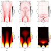 |
Fig. 1. Top row: Spatial distribution of |

We show the spatial distribution of the magnetic field lines projected in the xy plane (top row) and the absolute value of the guide field component (bottom row) in Fig. 1 for three different times: at the beginning of the semi-equilibrium phase (t = 5.44 min) and the two eruption phases respectively at t = 7.51 and 12.59 min. The central part of the arcade leads to the formation of a vertical current sheet (CS) when the field lines (By component with opposite polarity) come into close proximity to each other near the PIL, as seen in other flux rope eruption models (e.g., Ruan et al. 2020; Zhang et al. 2021; Dahlin et al. 2022) and inferred in the flare and coronal mass ejection observations (Reva et al. 2016; Yan et al. 2018; Patel et al. 2020). Concurrently, to trace the development of CS, we show the spatial distribution of |J|/B| as a proxy (where J is the electric current density) in the top row in Fig. 1. Here, eventual developments of the CSs around x = 3.14 Mm can be seen by the dark gray regions in the Figs. 1b and 1c.
After the semi-equilibrium phase at around t = 7 min, the field lines that are in proximity to the vertical CS region allow for a reconnection in a tether-cutting fashion (Antiochos et al. 1999; Moore et al. 2001). The presence of the guide field in those CS regions indicates a 2.5D reconnection (unlike a purely 2D reconnection); this was also reported in Sen & Moreno-Insertis (2025) regarding plasmoid instability in a coronal CS. This process adds a twist to the field lines above the reconnection point to form a magnetic flux rope, and increases the magnetic tension of the underlying loops. This process separates the flux rope from the underlying arcades and leads to the first eruption at around t = 7.51 min, shown in Fig. 1b. The flux rope holds the shear flux trapped within it (Fig. 1e) and transports it through the flux rope eruption. As a consequence of the reconnection, the post reconnection loops shrink down, carrying the shear flux within it, and contribute flux to the underlying arcades.
Afterward, due to the periodic condition at the horizontal boundaries, a pair of (straddling) flux ropes are also formed at t ≈ 10 min at the side boundaries (shown in Figs. 1(c) and 1(d) in S24). They erupt and leave the simulation box at t ≈ 11.8 min (see the animation associated with Fig. 1 in S24). During the eruption of these (side) flux ropes, nearly horizontal magnetic fields are created at the upper and the lower parts of these erupting ropes that have opposite and the same directions, respectively, to the underlying central arcade. The interaction of these side ropes with the remaining central arcade gradually leads to the formation of another flux rope and leads to the second eruption (from the central arcade region) at around t = 12.59 min (shown in Fig. 1c), which occurs in a fashion similar to the first eruption. The interaction of the lateral arcades can be seen from the high |J|/|B| regions in Figs. 1b and 1c. The study by Cheng & Choe (2001) also demonstrated the similar fact that a continuous increase of magnetic shear in the underlying arcades can trigger the reconnection process and leads to the formation of magnetic islands. After the second eruption phase, we did not observe any more flux rope formation at the central arcade region, as there is no sufficient shear in the underlying loops that can lead to the process.
To appreciate the spatial orientation of the magnetic field lines and the distribution of shear along the magnetic field lines, we present the 3D views of the field lines in Fig. 2. The top and bottom rows display the side and top views of the configurations, respectively, at t = 5.44, 7.51 and 12.59 min. In Fig. 2(a), the highly sheared segments of the central arcade, highlighted in red, become squeezed toward the PIL at t = 7.51 min (Fig. 2(b)). In Figs. 2(b) and (c), the portions of the field lines located near the PIL that are marked in red are highly sheared magnetic structures, and they are nearly parallel to the PIL. These magnetic structures contribute to the formation of channels that are capable of supporting filament materials, as reported in Zhao et al. (2015), Knizhnik et al. (2015, 2017) and references therein. These sheared portions of the field lines also play a role in the development of vertical CSs, which form beneath the flux ropes during the eruption phases at t = 7.51 and 12.59 min (see Figs. 1b, and 1c). The corresponding top views at t = 5.44, 7.51, and 12.59 min are shown in the bottom row, where the concentration of highly sheared field lines near the PIL are evident.
 |
Fig. 2. Variation of the shear angle along the magnetic field lines from the central arcade region for t = 5.44, 7.51, and 12.59 min (from left to right columns) obtained from simulation 1. The different shear angles (in degrees) are shown in different colors. The top and bottom rows represent the side and top views of the field line configurations. The 2D slices show the spatial variation of By in the x − z plane at the base of the simulation box, and values of By are shown by the color bar common for all the panels. The orientation of the x, y, z axes are shown in red, green, and blue arrows, respectively. For better visualization of the field lines, fewer field lines are shown in the bottom panels compared to the corresponding top panels. |
Further, to qualitatively investigate the distribution of the shear angle along the field lines, we traced the magnetic field lines from selected footpoints at the bottom boundary and estimated the shear angle along those field lines. This was done by integrating the magnetic field line equation by a third-order Runge-Kutta method from a footpoint until it reaches a boundary of the simulation domain, where the integration terminates. We also set a marker in the field line tracer routine to verify whether the integration terminates at the bottom boundary after tracing the field line from a given footpoint (i.e., the seed point at the bottom boundary), indicating a closed loop. Conversely, if the field line tracer terminates at any of the side or top boundaries, it is identified as an open loop. We present the selected field lines, shown in red and blue, for t = 7.51 min and 12.52 min in Figs. 3a and 3b, respectively, where the footpoints (or seed points marked in red and blue circles) are located at the bottom boundary (y = 0) at x = 1.61 and 2 Mm, which we call “footpoint 1” (FP1) and “footpoint 2” (FP2), respectively. The motivation for selecting these two footpoints is to trace field lines from the central arcade region that reconnect during the first and second eruption phases, respectively. We used a spatial coordinate, s, which is defined as the distance between the specific footpoints (namely, FP1 and FP2) and an arbitrary position at the corresponding field lines.
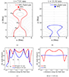 |
Fig. 3. (a) Distribution of magnetic field lines (in gray) for the entire spatial domain of simulation 1 at t = 7.51 min. The red curve represents the field line that is anchored at the seed point (footpoint) location (x, y) = (1.61, 0) Mm (FP1), marked by the red circle. (b) Same as the top-left panel but for t = 12.52 min. The blue field line is anchored at the seed point location (x, y) = (2, 0) Mm (FP2). (c) The red and the blue curves represent the distribution of the shear, γ, along the red and blue field lines as shown in the top-left and top-right panels, respectively. The vertical dashed lines are the positions along the red field line marked by the gray dots (s1, ..,s4) at the top-left panel. (d) Distribution of γ along the field lines anchored at FP1 (red curve) and FP2 (blue curve) at the beginning of the semi-equilibrium phase at t = 5.44 min. |
The distribution of the shear angle along the field lines anchored at FP1 and FP2 are shown in Fig. 3c for two instances of time of the first and the second eruption phases. In the figure, we have normalized the total length of the field lines to unity. We note that the shear along the field lines is distributed in a quite inhomogeneous fashion and with a (nearly) left-right symmetry from the apexes (i.e., at s = 0.5) of the respective loops for the two eruption phases. To map the one-to-one correspondence of shear at different locations along the field line for the first eruption phase, we selected four locations, namely, s1, s2, s3, and s4. These locations are marked by gray dots in Fig. 3a.
We noticed a strong shear (≈80°) at FP1 (at the location s0), marked by the red circle in Fig. 3a. Along the field line from s0, the shear falls sharply to ≈30° at s1 (s = 0.1) as a consequence of predominance of the horizontal component over its guide field. The magnetic field is in an approximately relaxed state just before the flux rope formation, and it follows a nearly magnetostatic equilibrium, and thus it follows as Bz(Az) (where, Az is the z-component of the magnetic vector potential associated with B). The constant Az also defines the field lines projected in the x − y plane. This is also evident from Figs. 1b and 1e, where the Bz strength follows (nearly) the field lines. Therefore, the distribution of the magnetic shear along the FP1 field line is (mostly) governed by the Bx component, as Bz remains nearly uniform along the field line. Hence, a smaller Bx corresponds to a higher shear, and a higher Bx corresponds to a smaller shear along that field line.
The shear reaches its maximum value (γ = 90°) at s2 (s ≈ 0.15), which is the upstream location of the CS, where the field lines are not yet reconnected and mostly vertical when projected in the x − y plane. We noticed a similar behavior at s3 (s = 0.32), where the shear reaches its peak value, which corresponds to the location of an incipient flux rope that is just about to form. Finally, s4, which is located at the apex of the incipient flux rope, shows a sufficiently strong shear of ≈75°. We repeated the calculation of estimating γ for the second eruption phase (t = 12.52 min). In this case, we noticed that the shears at the left and the right footpoints (x = 2, and 4.28 Mm, respectively, at y = 0) are weak (γ ≲ 15°) but comprise a stronger shear at the upper part of the loop, reaching a maximum value of ≈90° at s ≈ 0.32 and 0.68, which are marked as gray dots in Fig. 3b. These gray dots are the parts of an incipient flux rope for the second eruption phase.
The formation of the first flux rope occurs at a higher height than the second one (see Figs. 1b and 1c). To investigate the reason for this, we estimated the shear distribution at the beginning of the semi-equilibrium phase (t = 5.44 min) along the field lines connected to the same two footpoints, namely FP1 and FP2. For convenience, we refer to the field lines as the FP1 field line and the FP2 field line. From Fig. 3d, we noticed that the shear at FP1 and FP2 is the same (around 70°), and the FP2 field line has a nearly uniform shear. On the other hand, the shear along the FP1 field line is much more inhomogeneous and has a stronger shear at the upper part of the field line (0.15 ≲ s ≲ 0.85). Though the shear was spatially uniform at the initial stage (t = 0), the occurrence of reconnections before the beginning of the semi-equilibrium stage (t < 5.44 min, not shown) induces the inhomogeneity in shear distribution at the FP1 field line at the beginning of the semi-equilibrium phase. This higher shear at the upper part of the FP1 field line facilitates the formation of a flux rope at an earlier stage and at a higher height (y ≈ 17 Mm) compared to the formation of the flux rope from the FP2 field line.
Due to the strong inhomogeneity of shear that might appear along the field lines (as mentioned earlier), we estimated the mean shear along the field line ( ), which we refer as “mean shear” for convenience. This was estimated by integrating the shear angle along the field line and then dividing by the length of the field line:
 (7)
(7)
We calculated the temporal variation of  for the FP1 and FP2 field lines and present the result in Fig. 4a. At the semi-equilibrium phase, the mean shear of the FP1 field line is approximately 80° and gradually decreases until t = 7.51 min. During this period, the closed magnetic loop anchored to FP1 rises and stretches, corresponding to the elongation of the loop (shown by the red curve in Fig. 5). Overall, the loop becomes more perpendicular to the PIL, which leads to the decrease of the non-potentiality and hence the mean shear. The result is consistent with the study by Qiu et al. (2017), where they reported that the elongation of the loop, which was measured by the distance between the loop footpoints, reduces the shear during a flare evolution. The mean shear angle reaches 73° at around t = 7.51 minutes, as indicated by the vertical dashed gray line in the Fig. 4a. Shortly afterward, an upper part of the loop reconnects to form a flux rope at t = 7.58 min, and the remaining bottom part shrinks downward, forming an underlying arcade, which we call a post-reconnection loop. The shear flux carried by the flux rope is expelled upward during the eruption, resulting in a loss of free energy. We refer to Fig. 1 in S24 for the time series of the free to potential-field energy ratio capturing the time span of the first and second eruption phases, where one can see how the ratio drops during those time periods.
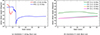 |
Fig. 4. (a) Temporal variation of the mean shear ( |


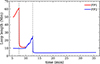 |
Fig. 5. Temporal variation of the total arcade length anchored at FP1 (red curve) and FP2 (blue curve) for simulation 1. The left and right vertical dashed lines are the time markers for t = 7.51 and 12.52 min, respectively. |
Due to the reconnection, the length of the closed field line (which is anchored at FP1) decreases from around 60 Mm at t = 7.51 min to 10 Mm at t ≈ 8.3 min (red curve in Fig. 5). As a consequence, there is a sharp drop in the mean shear of the FP1 field line in the newly formed post-reconnection loop beneath the erupting rope to approximately 55° at t = 8.3 min. Meanwhile, the shear flux that is transported downward by the shrinking field lines increases the magnetic flux of the underlying loops. This enhances the non-potentiality of those underlying arcades, and consequently, the mean shear gradually increases between t = 8.3 and 9.9 min (Fig. 4a). We did not extend the calculation beyond this time, as the field line tracer traces a neighboring (open) field line from FP1 shortly afterward that belongs to a different loop family that extends outward (to the left) of the central arcade.
We carried out the calculation for the field line that is anchored to FP2, and we present the result in Fig. 4a. Here, we noticed that the mean shear is around 72° and remains nearly same from the start of the semi-equilibrium phase (t = 5.44 min) until t ≈ 10 min. In this phase, the loop length remains nearly constant to 10 Mm (blue curve in Fig. 5). The tiny variations of the mean shear and loop length between t ≈ 11 and 12 min are due to the flickering nature of the loop, which is caused by the periodic boundary condition and the straddling half loops at the sides. Shortly after t = 10 min, during the onset of the second eruption phase, the loop length starts to increase, reaching around 25 Mm at t ≈ 12.52 min and lowering the non-potentiality of the loop similar to the case of the FP1 field line, as described above. Therefore, the mean shear drops to around 60° at that time. Right after t = 12.52 min, when a part of that field line reconnects to form an erupting flux rope, we observed a sharp drop of mean shear to ≈25°, and the field line length decreased to around 4 Mm. This length remains almost constant until the end of the evolution.
The shear flux carried downward contributes to the flux in the underlying loops in a manner similar to what occurs in the first post-eruption phase, and we observed a gradual increment of the mean shear (blue curve at the Fig. 4a). This value reaches ≈48° at t ≈ 20 min. After this stage, there is no more significant shear flux injected into the underlying loop, and therefore the mean shear remains almost constant until the end of the evolution. The amount of shear remaining at the central loops after this is not sufficient to form flux ropes from the central arcade region.
We investigated the temporal variation of the mean shear for simulation 2, which has a weaker (spatially uniform) shear (γ = 25.8°) than simulation 1 (γ = 72.5°) at the initial time. To do so, we traced the field lines of the central loop from different footpoint locations of (x, y) = [(1.6, 0),(1.8, 0),(2, 0),(2.2, 0)] Mm and estimated  as described above. We noticed that the mean shear angle of the field line from the footpoint location (1.6, 0) Mm is at a maximum, which is around 45°, and the angle remained nearly constant between the same time span of the evolution of simulation 1, as shown in Fig. 4b. However, we also noticed that field lines that are anchored with the other footpoints are closer to the PIL (at x = 3.14 Mm) and have a weaker shear and that
  varies between ≈28° to 36° during the evolution. In this case, the shear present in any of the field lines of the central arcade region is not sufficient to trigger the formation of a flux rope, and it remains in a quasi-stationary state until the end of the evolution.
To investigate the temperature evolution of the pre- and post-reconnection loops, we estimated the mean temperature along the field line in a manner similar to the  in Eq. (7):
 (8)
(8)
The result is presented in Fig. 6. Here, we focus on the results pertaining specifically to the second eruption phase. To this end, we selected the magnetic field lines anchored at FP2 (i.e., [x, y]=[2, 0] Mm) in order to estimate the evolution of the mean temperature,  , capturing both the pre- and post-eruption temporal domains. In the case of weak shear (simulation 2), no significant change was observed in the temperature (
 ) evolution, which remains at around 1 MK (which is the same as the initial iso-thermal condition) throughout the evolution. In contrast, for the strong shear case (simulation 1),
  exhibits substantial variation, ranging approximately from 0.8 to 2.3 MK.
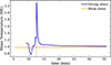 |
Fig. 6. Time evolution of mean temperature, |

During the interval between t = 9.3 and 11 min, the temperature decreases from about 1.1 MK to 0.8 MK. During this pre-reconnection phase, the stretching of the loop leads to an increase of thermal conduction timescale (which varies ∼L2, where, L is the characteristic length scale of the loop). This means the thermal conduction becomes less efficient than a shorter length scale scenario. Therefore, the thermal conduction cannot react faster to increase the temperature than the cooling mechanism that is facilitated mostly by adiabatic expansion of the loops. Subsequently,  rises to approximately 2.3 MK at t ≈ 12.5 min, primarily due to ohmic heating in the region of enhanced current density at the vertical CS (see Fig. 1c). Shortly thereafter, at t = 12.6 min, the mean temperature of the post-reconnection loop begins to decrease again, reaching the initial temperature of around 1 MK by t ≈ 15 min, and it remains at that level through to the end of the evolution at around t = 35 min. This temperature decline is attributed to the downward transport of thermal energy along the loop caused by thermal conduction. Notably, the fast temperature change (with a timescale of about a few minutes) during the transition phase from the reconnection to post-reconnection period (between t = 12.6 to 15 min) is governed by the small length scale of the loop (about a few Mm), which corresponds to a small thermal conduction timescale, as well as the temperature inhomogeneities present along the loop.
The relative strength between the reconnection field and the guide field components at the upstream location in a CS can be a deciding factor in particle acceleration and bulk heating (Dahlin et al. 2022; Qiu et al. 2023). To assess this mechanism, we estimated the time evolution of the ratio between the guide and vertical magnetic field components, defined as RCS = −Bz/By, at the right side (x > 3.14 Mm) of the upstream region of the CS during the two eruption phases (at t = 7.51 and 12.59 min). At this upstream location, By consistently remains negative in our case (i.e., directed downward), whereas Bz can vary between positive and negative values. Thus, the adopted convention of RCS helps identify when the guide field component at this location changes polarity. To perform our analysis, we first selected a vertical span encompassing the CS that is present at x = 3.14 Mm and identified the pixel within this region that corresponds to the maximum value of |J|/B|. This was also crosschecked with the maps in Figs. 1b and 1c. We then took a horizontal cut of the quantity |J|/B| that passes through to that specific pixel with peak |J|/B|, as shown by the black curves in Fig. 7 for t = 7.51 and 12.59 min, respectively. To determine the upstream locations on the right side of the evolving CS, we selected the pixels that reach 50% of the instantaneous peak value of |J|/B| while moving right along the x-direction from x = 3.14 Mm. These upstream positions are marked by gray vertical dashed lines in the left and right panels of Fig. 7 for the first and second eruption phases, respectively. The reconnecting (By) and the guide (Bz) field profiles are also overplotted in the figure to show the consistency of the CS structure. Using this automated technique, we estimated the temporal evolution of RCS and present the results in Fig. 8.
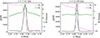 |
Fig. 7. Spatial distribution of |J|/B| (black), vertical component (magenta), and guide field component (green) along the horizontal direction that passes through the CS at y = 10 Mm and y = 3 Mm for the first (t = 7.51 min; left figure) and second (t = 12.59 min; right figure) eruption phases, respectively. |
The left and right panels of Fig. 8 correspond to the time span that captures the first and second eruption phases, respectively. During the pre-eruption phases, RCS is more than unity, indicating that the guide field is stronger than the reconnection field component. In these periods, plasmoid-driven particle acceleration should be suppressed and fewer nonthermal electrons should be produced due to a weakened Fermi-type mechanism, as suggested in Arnold et al. (2021). However, during the late phase of eruption, when RCS decreases toward zero, the reconnection field component becomes dominant over the guide field. At this stage, the energy contribution from non-thermal electrons exceeds that of hot thermal electrons, resulting in efficient particle acceleration, as proposed by Dahlin et al. (2016). This suggests that during the pre-eruption phases, the dominant guide field primarily drives bulk heating, whereas during the late phases of eruptions, the dominant reconnection field component facilitates the particle acceleration more efficiently. This estimation also gives a potential direction to explain the “hot onset” phenomena, where the bulk heating is observed prior to the efficient particle acceleration in flares, reported in Hudson et al. (2021).
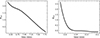 |
Fig. 8. Temporal variation of the guide to vertical magnetic field component ratio, RCS (= − Bz/By), at the upstream location of CS, marked by the vertical dashed lines in the left and right panels of Fig. 7, during the first (left panel) and second (right panel) eruption phases. |
4. Summary and discussion
We have presented the results from a 2.5D MHD model of multiple (homologous) flux rope eruptions (S24), focusing on the role of magnetic shear distribution in facilitating these eruptions. Specifically, we analyzed two cases with different values of initial magnetic shear (γ) but with all other parameters the same. In both cases, the system initially (at t = 0) exhibits mechanical imbalance. However, it transiently settles into a nearly force-free and thermally balanced semi-equilibrium state after approximately 5.44 min. Shortly after that, for the strong shear case (γ = 72.6°, simulation 1), the system produces two flux ropes from the central arcade region, and they erupt at around 7.51 and 12.59 min. In contrast, the weak shear case (γ = 25.8°, simulation 2) does not show any flux rope formation after it reaches the semi-equilibrium phase, and it remains in a quasi-stationary state thereafter. These results suggest that magnetic shear in the arcades due to presence of the guide field plays an intrinsic role in the formation and eruption of flux ropes. In this work, we have focused on the formation and eruption of the flux ropes only from the central arcade region, and we did not pay attention to the (partial) flux ropes formed at the side boundaries due to the initial magnetic field prescription and periodic boundary condition (see S24 for more details).
The initial shear was spatially uniform in the entire simulation domain, but a nonuniformity developed in the field lines at the beginning of the semi-equilibrium phase, as the stage before the semi-equilibrium phase (t < 5.44 min) consists of reconnections (not shown) due to the presence of Lorentz force. Formation of the first flux rope occurs at a higher height than the second one because at the beginning of the semi-equilibrium phase, the field lines that are connected with the outer legs (away from the PIL) of the arcade consist of more shear at a higher height than the field lines from the inner legs. The field lines in the vicinity of the vertical CS are highly sheared and nearly parallel to the PIL. These are the parts of the field lines that reconnect. This implies that the amount of shear flux that is ejected upward by the eruptive flux ropes and the residual flux that is transported downward to the post reconnection loops are both decided by the location of reconnection on the arcade.
During the pre-eruption phase, a gradual decrease in the mean shear ( ) of the field lines is associated with the stretching of magnetic loops, which continues until magnetic reconnection occurs. Following the reconnection event, part of the arcade structure forms a flux rope that erupts and carries the shear flux with it, while the remaining portion of the arcade becomes the post-reconnection loop. Consequently, the mean shear of the reconnecting loop drops drastically just after the reconnection. In other words, a sudden drop of mean shear of a flaring loop may indicate a reconnection event. After the eruption, the downward-transported residual shear flux contributes to the magnetic flux in the underlying arcades, leading to a gradual increment in non-potentiality. Observationally, estimating mean shear along field lines is extremely challenging, if not impossible. However, temporal variations of magnetic shear at the photosphere are measurable and have been reported for various flare events. For example, according to the study by Gosain & Venkatakrishnan (2010), the horizontal shear (referred to as the “dip shear”) at the sunspot penumbra regions decreases following an X-class flare. Petrie (2019) reported a reduction in shear during a flare in an active region. Moreover, Magara (2009) found that shear decreases even before the onset of an X-class flare. Though the trend of the mean shear obtained from our study and the photospheric shear for different flare observations follows a similar pattern, the one-to-one correspondence between these two quantities cannot be established across different phases of the eruption. Still, the similar trends between our numerical study and the existing observations encourage further investigations to explore any potential correlation between the evolution of the photospheric magnetic shear and the mean magnetic shear along the coronal arcades during pre- and post-eruptive phenomena.
This work highlights the possibility of fast temperature evolution (on timescales of approximately a few minutes) during the pre-reconnection, and the transition period between the reconnection to post-reconnection phases for small-scale flare-associated loops. Our findings thus motivate observational investigations aimed at confirming this scenario.
This study also sheds light on the understanding of energy release processes during an eruptive flare. According to the studies by Dahlin et al. (2016), Arnold et al. (2021), it has been demonstrated that the strong guide field suppresses the plasmoid-driven particle acceleration. The bulk heating on the other hand, which refers to the increase in thermal energy of the plasma (raising the temperature of the entire ion and electron population) is (mostly) insensitive to the guide field. Therefore, we expect that the plasma heating should dominate over the particle acceleration during the onset phase of the eruptions when the strength of the guide field dominates over the reconnection field component, which might serve as a potential clue for a better understanding of the “hot onset” phenomena in flare observations (Hudson et al. 2021). On the other hand, during the late phase of the eruption stage, when the reconnection field component dominates over the guide field, we expect a more efficient particle acceleration.
This work primarily highlights the role of magnetic shear distribution in the formation and eruption of multiple flux ropes within a 2.5D Cartesian geometry. The eruptions in our model emerge without any driving agent beyond the initial (mechanically imbalanced) conditions, unlike Dahlin et al. (2022), for example, where shear flow was injected at the bottom boundary in a relaxed system. However, an extension of this work in a 3D geometry starting from the equilibrium configuration for a local box simulation with coupling to the lower atmospheres and for a large-scale global model can be an interesting aspect to investigate in the future. Nevertheless, this study demonstrates that the distribution and variability of the guide field is an inevitable quantity that triggers the formation and eruption of flux ropes and energy release (through bulk heating and particle acceleration) in the Sun, which are essential to resolve the broader coronal heating mystery.
Acknowledgments
SS acknowledges support by the European Research Council through the Synergy Grant #810218 (“The Whole Sun”, ERC-2018-SyG). He thankfully acknowledges the technical expertise and assistance provided by the Spanish Supercomputing Network (Red Española de Supercomputación), as well as the computer resources used: the LaPalma Supercomputer, located at the Instituto de Astrofísica de Canarias. We would like to thank the anonymous referee for the insightful and useful comments that improved the manuscript considerably. We would like to thank Joel Dahlin, David Pontin, and James Klimchuk for useful discussions. Data visualization and analysis were performed using Python 3.11.9, yt-project, visit 2.10, and Vapor 3. SSN acknowledges the supports from NSF-AGS-1954503, NASA-LWS- 80NSSC21K0003, and 80NSSC21K1671 grants and the I+D+i project PID2023-147708NB-I00 funded by MICIU/AEI/10.13039/501100011033/ and by FEDER, EU.
References
- Antiochos, S. K. 1998, ApJ, 502, L181 [Google Scholar]
- Antiochos, S. K., DeVore, C. R., & Klimchuk, J. A. 1999, ApJ, 510, 485 [Google Scholar]
- Arnold, H., Drake, J. F., Swisdak, M., et al. 2021, Phys. Rev. Lett., 126, 135101 [NASA ADS] [CrossRef] [Google Scholar]
- Aulanier, G., Janvier, M., & Schmieder, B. 2012, A&A, 543, A110 [NASA ADS] [CrossRef] [EDP Sciences] [Google Scholar]
- Cheng, C. Z., & Choe, G. S. 2001, Earth Planets Space, 53, 597 [Google Scholar]
- Cheng, C. Z., Ren, Y., Choe, G. S., & Moon, Y. J. 2003, ApJ, 596, 1341 [Google Scholar]
- Chifor, C., Young, P. R., Isobe, H., et al. 2008, A&A, 481, L57 [NASA ADS] [CrossRef] [EDP Sciences] [Google Scholar]
- Dahlin, J. T., Drake, J. F., & Swisdak, M. 2016, Phys. Plasmas, 23, 120704 [Google Scholar]
- Dahlin, J. T., Antiochos, S. K., Qiu, J., & DeVore, C. R. 2022, ApJ, 932, 94 [CrossRef] [Google Scholar]
- Démoulin, P., & Pariat, E. 2009, Adv. Space Res., 43, 1013 [CrossRef] [Google Scholar]
- Ding, J. Y., Hu, Y. Q., & Wang, J. X. 2006, Sol. Phys., 235, 223 [NASA ADS] [CrossRef] [Google Scholar]
- Gosain, S., & Venkatakrishnan, P. 2010, ApJ, 720, L137 [Google Scholar]
- Hagyard, M. J., & Rabin, D. M. 1986, Adv. Space Res., 6, 7 [Google Scholar]
- Hagyard, M. J., Smith, J. B., Jr, Teuber, D., & West, E. A. 1984, Sol. Phys., 91, 115 [Google Scholar]
- Hong, J., Jiang, Y., Zheng, R., et al. 2011, ApJ, 738, L20 [Google Scholar]
- Hudson, H. S., Simões, P. J. A., Fletcher, L., Hayes, L. A., & Hannah, I. G. 2021, MNRAS, 501, 1273 [Google Scholar]
- Inoue, S., Kusano, K., Magara, T., Shiota, D., & Yamamoto, T. T. 2011, ApJ, 738, 161 [Google Scholar]
- Keppens, R., Nool, M., Tóth, G., & Goedbloed, J. P. 2003, Comp. Phys. Commun., 153, 317 [Google Scholar]
- Keppens, R., Meliani, Z., van Marle, A. J., et al. 2012, J. Comput. Phys., 231, 718 [Google Scholar]
- Keppens, R., Teunissen, J., Xia, C., & Porth, O. 2021, Comput. Math. Appl., 81, 316 [Google Scholar]
- Keppens, R., Popescu Braileanu, B., Zhou, Y., et al. 2023, A&A, 673, A66 [NASA ADS] [CrossRef] [EDP Sciences] [Google Scholar]
- Kliem, B., & Török, T. 2006, Phys. Rev. Lett., 96, 255002 [Google Scholar]
- Knizhnik, K. J., Antiochos, S. K., & DeVore, C. R. 2015, ApJ, 809, 137 [NASA ADS] [CrossRef] [Google Scholar]
- Knizhnik, K. J., Antiochos, S. K., DeVore, C. R., & Wyper, P. F. 2017, ApJ, 851, L17 [Google Scholar]
- Kumar, S., Bhattacharyya, R., Joshi, B., & Smolarkiewicz, P. K. 2016, ApJ, 830, 80 [NASA ADS] [CrossRef] [Google Scholar]
- Lu, Y., Wang, J., & Wang, H. 1993, Sol. Phys., 148, 119 [Google Scholar]
- Lu, Z., Chen, F., Guo, J. H., et al. 2024, ApJ, 973, L1 [Google Scholar]
- MacTaggart, D., Prior, C., Raphaldini, B., Romano, P., & Guglielmino, S. L. 2021, Nat. Commun., 12, 6621 [NASA ADS] [CrossRef] [Google Scholar]
- Magara, T. 2009, ApJ, 702, 386 [Google Scholar]
- McGlasson, R. A., Panesar, N. K., Sterling, A. C., & Moore, R. L. 2019, ApJ, 882, 16 [NASA ADS] [CrossRef] [Google Scholar]
- Mikic, Z., Barnes, D. C., & Schnack, D. D. 1988, ApJ, 328, 830 [Google Scholar]
- Moore, R. L., Sterling, A. C., Hudson, H. S., & Lemen, J. R. 2001, ApJ, 552, 833 [Google Scholar]
- Moreno-Insertis, F., Galsgaard, K., & Ugarte-Urra, I. 2008, ApJ, 673, L211 [Google Scholar]
- Nayak, S. S., Sen, S., Shrivastav, A. K., Bhattacharyya, R., & Athiray, P. S. 2024, ApJ, 975, 143 [Google Scholar]
- Panesar, N. K., Sterling, A. C., & Moore, R. L. 2016, ApJ, 822, L23 [NASA ADS] [CrossRef] [Google Scholar]
- Panesar, N. K., Sterling, A. C., & Moore, R. L. 2018, ApJ, 853, 189 [NASA ADS] [CrossRef] [Google Scholar]
- Patel, R., Pant, V., Chandrashekhar, K., & Banerjee, D. 2020, A&A, 644, A158 [NASA ADS] [CrossRef] [EDP Sciences] [Google Scholar]
- Patty, S. R., & Hagyard, M. J. 1986, Sol. Phys., 103, 111 [Google Scholar]
- Peter, H., Bingert, S., Klimchuk, J. A., et al. 2013, A&A, 556, A104 [NASA ADS] [CrossRef] [EDP Sciences] [Google Scholar]
- Petrie, G. J. D. 2019, ApJS, 240, 11 [NASA ADS] [CrossRef] [Google Scholar]
- Porth, O., Xia, C., Hendrix, T., Moschou, S. P., & Keppens, R. 2014, ApJS, 214, 4 [Google Scholar]
- Qiu, J., Longcope, D. W., Cassak, P. A., & Priest, E. R. 2017, ApJ, 838, 17 [Google Scholar]
- Qiu, J., Alaoui, M., Antiochos, S. K., et al. 2023, ApJ, 955, 34 [Google Scholar]
- Reva, A. A., Ulyanov, A. S., & Kuzin, S. V. 2016, ApJ, 832, 16 [Google Scholar]
- Ruan, W., Xia, C., & Keppens, R. 2020, ApJ, 896, 97 [NASA ADS] [CrossRef] [Google Scholar]
- Schmieder, B., Demoulin, P., Aulanier, G., & Golub, L. 1996, ApJ, 467, 881 [Google Scholar]
- Sen, S., & Moreno-Insertis, F. 2025, A&A, 699, A106 [NASA ADS] [CrossRef] [EDP Sciences] [Google Scholar]
- Sen, S., Prasad, A., Liakh, V., & Keppens, R. 2024, A&A, 688, A64 [NASA ADS] [CrossRef] [EDP Sciences] [Google Scholar]
- Shibata, K., Ishido, Y., Acton, L. W., et al. 1992, PASJ, 44, L173 [Google Scholar]
- Shibata, K., Nakamura, T., Matsumoto, T., et al. 2007, Science, 318, 1591 [Google Scholar]
- Sivaraman, K. R., Rausaria, R. R., & Aleem, S. M. 1992, Sol. Phys., 138, 353 [Google Scholar]
- Soenen, A., Zuccarello, F. P., Jacobs, C., et al. 2009, A&A, 501, 1123 [NASA ADS] [CrossRef] [EDP Sciences] [Google Scholar]
- Sterling, A. C., Moore, R. L., Falconer, D. A., Panesar, N. K., & Martinez, F. 2017, ApJ, 844, 28 [NASA ADS] [CrossRef] [Google Scholar]
- Török, T., Kliem, B., & Titov, V. S. 2004, A&A, 413, L27 [NASA ADS] [CrossRef] [EDP Sciences] [Google Scholar]
- Xia, C., Teunissen, J., El Mellah, I., Chané, E., & Keppens, R. 2018, ApJS, 234, 30 [Google Scholar]
- Yan, X. L., Yang, L. H., Xue, Z. K., et al. 2018, ApJ, 853, L18 [Google Scholar]
- Yeates, A. R. 2024, Sol. Phys., 299, 83 [Google Scholar]
- Young, P. R., & Muglach, K. 2014, PASJ, 66, S12 [Google Scholar]
- Zhang, Q., Liu, R., Wang, Y., et al. 2021, A&A, 647, A171 [NASA ADS] [CrossRef] [EDP Sciences] [Google Scholar]
- Zhao, L., DeVore, C. R., Antiochos, S. K., & Zurbuchen, T. H. 2015, ApJ, 805, 61 [NASA ADS] [CrossRef] [Google Scholar]
- Zhao, X., Xia, C., Keppens, R., & Gan, W. 2017, ApJ, 841, 106 [Google Scholar]
All Figures
|
Fig. 1. Top row: Spatial distribution of |
| In the text | |
|
Fig. 2. Variation of the shear angle along the magnetic field lines from the central arcade region for t = 5.44, 7.51, and 12.59 min (from left to right columns) obtained from simulation 1. The different shear angles (in degrees) are shown in different colors. The top and bottom rows represent the side and top views of the field line configurations. The 2D slices show the spatial variation of By in the x − z plane at the base of the simulation box, and values of By are shown by the color bar common for all the panels. The orientation of the x, y, z axes are shown in red, green, and blue arrows, respectively. For better visualization of the field lines, fewer field lines are shown in the bottom panels compared to the corresponding top panels. |
| In the text | |
|
Fig. 3. (a) Distribution of magnetic field lines (in gray) for the entire spatial domain of simulation 1 at t = 7.51 min. The red curve represents the field line that is anchored at the seed point (footpoint) location (x, y) = (1.61, 0) Mm (FP1), marked by the red circle. (b) Same as the top-left panel but for t = 12.52 min. The blue field line is anchored at the seed point location (x, y) = (2, 0) Mm (FP2). (c) The red and the blue curves represent the distribution of the shear, γ, along the red and blue field lines as shown in the top-left and top-right panels, respectively. The vertical dashed lines are the positions along the red field line marked by the gray dots (s1, ..,s4) at the top-left panel. (d) Distribution of γ along the field lines anchored at FP1 (red curve) and FP2 (blue curve) at the beginning of the semi-equilibrium phase at t = 5.44 min. |
| In the text | |
|
Fig. 4. (a) Temporal variation of the mean shear ( |
| In the text | |
|
Fig. 5. Temporal variation of the total arcade length anchored at FP1 (red curve) and FP2 (blue curve) for simulation 1. The left and right vertical dashed lines are the time markers for t = 7.51 and 12.52 min, respectively. |
| In the text | |
|
Fig. 6. Time evolution of mean temperature, |
| In the text | |
|
Fig. 7. Spatial distribution of |J|/B| (black), vertical component (magenta), and guide field component (green) along the horizontal direction that passes through the CS at y = 10 Mm and y = 3 Mm for the first (t = 7.51 min; left figure) and second (t = 12.59 min; right figure) eruption phases, respectively. |
| In the text | |
|
Fig. 8. Temporal variation of the guide to vertical magnetic field component ratio, RCS (= − Bz/By), at the upstream location of CS, marked by the vertical dashed lines in the left and right panels of Fig. 7, during the first (left panel) and second (right panel) eruption phases. |
| In the text | |
Current usage metrics show cumulative count of Article Views (full-text article views including HTML views, PDF and ePub downloads, according to the available data) and Abstracts Views on Vision4Press platform.
Data correspond to usage on the plateform after 2015. The current usage metrics is available 48-96 hours after online publication and is updated daily on week days.
Initial download of the metrics may take a while.