| Issue |
A&A
Volume 703, November 2025
|
|
|---|---|---|
| Article Number | A303 | |
| Number of page(s) | 16 | |
| Section | Galactic structure, stellar clusters and populations | |
| DOI | https://doi.org/10.1051/0004-6361/202556444 | |
| Published online | 26 November 2025 | |
The large-scale kinematics of young stars in the Milky Way disc: First results from SDSS-V
1
Dipartimento di Fisica e Astronomia, Università degli Studi di Firenze,
Via G. Sansone 1,
50019
Sesto F.no (Firenze),
Italy
2
Max-Planck-Institut für Astronomie,
Konigstuhl 17,
69117
Heidelberg,
Germany
3
Department of Physics and Astronomy, University of North Florida,
1 UNF Dr,
Jacksonville,
FL 32224,
USA
4
Canadian Institute for Theoretical Astrophysics, University of Toronto,
60 St. George Street,
Toronto,
ON M5S 3H8,
Canada
5
David A. Dunlap Department of Astronomy and Astrophysics, University of Toronto,
50 St. George Street,
Toronto,
ON M5S 3H4,
Canada
6
Institute of Astronomy, KU Leuven,
Celestijnenlaan 200D,
3001
Leuven,
Belgium
7
Leibniz-Institut für Astrophysik Potsdam (AIP),
An der Sternwarte 16,
14482
Potsdam,
Germany
8
University of Wisconsin–Madison, Department of Astronomy,
Madison,
WI 53706,
USA
9
Departamento de Astronomía, Facultad de Ciencias, Universidad de La Serena,
Av. Raul Bitran 1302,
La Serena,
Chile
10
Universidad Nacional Autónoma de México, Instituto de Astronomía,
AP 106, Ensenada
22800,
BC,
Mexico
11
University of Colorado Boulder,
Boulder,
CO 80309,
USA
12
Department of Astronomy, University of Virginia,
Charlottesville,
VA 22904,
USA
13
Department of Space, Earth & Environment,
Chalmers University of Technology,
41293
Gothenburg,
Sweden
14
Instituto de Astronomía, Universidad Nacional Autónoma de México, Unidad Académica en Ensenada,
Km 103 Carr. Tijuana-Ensenada,
Ensenada
22860,
Mexico
15
Apache Point Observatory and New Mexico State University,
PO Box 59, Sunspot,
NM 88349-0059,
USA
16
Sternberg Astronomical Institute, Moscow State University,
Moscow
119234,
Russia
17
Department of Physics and Astronomy, Texas Christian University,
Fort Worth,
TX 76129,
USA
18
Instituto de Astronomía, Universidad Católica del Norte,
Av. Angamos
0610,
Antofagasta,
Chile
19
Department of Astronomy, University of Illinois at Urbana-Champaign,
Urbana,
IL 61801,
USA
20
Instituto de Astronomía, Universidad Nacional Autónoma de México,
A.P. 70-264, 04510 Mexico,
D.F.,
Mexico
21
Department of Astrophysical Sciences, Princeton University,
Princeton,
NJ 08544,
USA
★ Corresponding author: This email address is being protected from spambots. You need JavaScript enabled to view it.
Received:
16
July
2025
Accepted:
1
October
2025
Abstract
We present a first large-scale kinematic map of ∼50 000 young OB stars (Teff ≥ 10 000 K), based on BOSS spectroscopy from the Milky Way Mapper OB programme in the ongoing Sloan Digital Sky Survey V (SDSS-V). Using photogeometric distances, line-of-sight velocities, and Gaia DR3 proper motions, we mapped 3D galactocentric velocities across the Galactic plane to ∼ 5 kpc from the Sun, with a focus on radial motions (vR). Our results reveal mean radial motion with amplitudes of ±30 km/s that are coherent on kiloparsec scales, alternating between inward and outward motions. These v̄R amplitudes are considerably higher than those observed for older red-giant populations. These kinematic patterns show only a weak correlation with spiral arm over-densities. Age estimates, derived from MIST isochrones, indicate that 85% of the sample is younger than ∼300 Myr and that the youngest stars (≤30 Myr) align well with density enhancements. The age-dependent v̄R in Auriga makes it plausible that younger stars exhibit different velocity variations than older giants. The origin of the radial-velocity features remains uncertain, and it may result from a combination of factors, including spiral-arm dynamics, the Galactic bar, resonant interactions, or phase mixing following a perturbation. The present analysis is based on approximately one-third of the full target sample. The completed survey will enable a more comprehensive investigation of these features and a detailed dynamical interpretation.
Key words: stars: early-type / Galaxy: disk / Galaxy: kinematics and dynamics / Galaxy: structure
© The Authors 2025
 Open Access article, published by EDP Sciences, under the terms of the Creative Commons Attribution License (https://creativecommons.org/licenses/by/4.0), which permits unrestricted use, distribution, and reproduction in any medium, provided the original work is properly cited.
This article is published in open access under the Subscribe to Open model. This email address is being protected from spambots. You need JavaScript enabled to view it. to support open access publication.
1 Introduction
The Galactic disc exhibits significant non-axisymmetric structures that fundamentally affect both stellar distributions and kinematics. Spiral arms and the Galactic bar constitute primary drivers of this non-axisymmetry, playing a crucial role in star formation processes and determining the morphological structure of the Milky Way (Antoja et al. 2018; Frankel et al. 2018; Reid et al. 2019; Eilers et al. 2020; Poggio et al. 2021).
Recent stellar density-mapping efforts have successfully traced segments of the Galactic spiral arms through the spatial distribution of stars. Multiple studies have utilised samples of upper-main-sequence (UMS) and OBA-type stars (Zari et al. 2021; Poggio et al. 2021; Gaia Collaboration 2023; Xu et al. 2023; Ge et al. 2024), A-type stars (Ardèvol et al. 2023), and red-clump (RC) stars (Lin et al. 2022). These analyses have consistently identified over-densities corresponding to the Perseus and Local Arms, as well as features associated with the Sagittarius-Scutum arm complex.
Kinematic analyses have revealed correlations between stellar-velocity fields and spiral structure. Gaia Collaboration (2023) demonstrated significant relationships between spiral-like over-densities and mean velocity fields in three dimensions (radial, azimuthal, and vertical) for their OB star sample within |z|<0.3 kpc and d ≤ 2 kpc. Their extended analysis incorporating red-giant-branch (RGB) stars revealed coherent large-scale velocity patterns, albeit with weaker correlations to spiral structure compared to the OB population. Eilers et al. (2020) identified a large-scale, galactocentric radial-velocity feature in their giant star sample, which can be interpreted as the response to a steady-state logarithmic spiral perturbation. Palicio et al. (2023) identified arc-shaped structures in the radial actions, JR, of a clean sample of Gaia DR3 stars with full astrometric information and line-of-sight velocities available. They suggested that these features could be a response to the spiral arms or the Galactic bar, or they could be connected to moving groups. With few exceptions (Gaia Collaboration 2023; Poggio et al. 2025), density mapping has mostly relied on ‘young’ samples (τage ≤ torbit), while kinematic studies of the Milky Way disc have been based on ‘old’ stars (τage ⋙ torbit). This is largely due to a lack of spectroscopic data for large samples of young stars, extending over a significant volume of the Galactic disc.
One of the core programmes of the current Sloan Digital Sky Survey incarnation (SDSS-V, Kollmeier et al. 2025, 2017; Almeida et al. 2023; SDSS Collaboration 2025) has set out to remedy this issue. The Milky Way Mapper OB core programme mwm_ob targets a large (∼ 0.5 million stars) sample of massive hot stars utilising the Baryon Oscillation Spectroscopic Survey (BOSS) spectrograph installed at the Apache Point Observatory (APO) in New Mexico, USA (Gunn et al. 2006) and the du Pont 2.5 m telescope at Las Campanas Observatory (LCO) in Chile (Bowen & Vaughan 1973). BOSS1 is an optical spectrograph covering a wavelength range of 3622−10 354 Å with a resolution of R ∼ 1800 (Smee et al. 2013). Zari et al. (2021) outlined the scientific goals of the mwm_ob program and presented the selection function of the target sample.
In this paper, we describe the properties of sample observed as of February 2025 and construct a large-scale kinematic map of the Galactic disc for young stars, which provides a novel view on the young Milky Way disc, different from what is seen for older populations. In Section 2, we summarise the selection function of the SDSS-V hot-star sample, focussing on the differences with respect to Zari et al. (2021) and Gaia Collaboration (2023). In Section 3, we compute the 3D velocities and ages for our sample members and construct a large-scale map of the galactocentric radial velocities, v̄R. We discuss our findings in Section 4 by comparing them with mock stellar catalogues generated from the AURIGA cosmological simulations and observations of older stellar populations. Finally, in Section 5 we draw our conclusions and discuss future work.
2 The SDSS-V hot-star sample
SDSS-V’s science is organised in mapper programs (Kollmeier et al. 2025; SDSS Collaboration 2025), including the Milky Way Mapper program, whose science in turn is parsed operationally in sample ‘cartons’. In this section, we describe the selection function of the mwm_ob target carton and the status of the observations as of 2 February 2025 (start of survey thru MJD=60708). We chose this date because it will be the cut for SDSS data release 20 (DR20), which is scheduled no earlier than June 2026. We present the criteria that we used to remove cooler sources from the initial mwm_ob targets after the spectra had been obtained, and the spectral parameters and line of sight velocities used.
2.1 Selection function of the SDSS-V mwm_ob targets
The targeting strategy of the mwm_ob sample in SDSS-V is presented in Zari et al. (2021, Z21). In Z21, the target-selection strategy prioritized completeness over purity, with the understanding that SDSS-V spectroscopic data would later allow us to refine the sample and improve its purity. The target selection relies on a combination of photometric and astrometric criteria based on Gaia E/DR3 and 2MASS (Skrutskie et al. 2006) astrometry and photometry. Z21’s target sample (described in their Section 2.1) consisted of stars more luminous than MK = 0 mag (where MK is the absolute magnitude in the 2MASS Ks band and ϖ indicates the parallax in mas), or, more precisely,
 (1)
(1)
In practice, the SDSS-V survey strategy (“Robostrategy”, Blanton et al. 2025) – and in particular the need to reduce the size of our sample from around 1 Ml to ∼0.5 Ml sources – required a slightly tighter selection:
 (2)
(2)
which corresponds to MK<−0.6 mag. The latter condition ideally selects stars of spectral type earlier than B3V (see e.g. Pecaut & Mamajek 2013). Between the start of the survey and 2 February 2025 (MJD 60708), SDSS-V obtained 459 679 spectra of 165 460 distinct targets in the mwm_ob program. Figure 1 (top) shows the distribution of sources in the sky (Galactic coordinates). Whilst the coverage is not uniform, much of the Galactic plane has already been observed, which allows for a first exploration of the global kinematic properties of the sample.
We compared our sample with the Gaia Collaboration (2023, D23) sample of O- and B-type stars. D23 (see Appendix A) selected sources based on their effective temperatures Teff,GSPPHOT and Teff,ESP−HS. The GSPPHOT temperature estimates are derived by combining Gaia GBP/GRP spectrophotometry, astrometry, and G-band photometry. The ESP-HS estimates are derived from a software module (ESP-HS) that was optimised specifically for hot stars and uses the BP/RP spectrophotometry, without the astrometry, together with the RVS spectra if they are available as well (Creevey et al. 2023; Fouesneau et al. 2023). For stars with only GSP-Phot temperatures, D23 used two conditions: Teff,GSPPHOT>10 000 K and the ESP-HS spectral type flag set to O, B, or A; for stars with only ESP-HS temperatures, they required that the effective temperature be in the range 10 000<Teff,ESPHS<50 000 K; for sources with both sets of stellar parameters, they required the effective temperature to be Teff,GSP−Phot>8000 K and Teff,ESPHSH> 10 000 K. These selection criteria resulted in a list of 923 700 sources.
Around 25% of the mwm_ob targets are in common with D23. The majority of the sources (90%) that are included in D23 but are not in the mwm_ob program are between −0.6<MK<2 mag, and they are thus excluded by our more stringent selection cuts (see Appendix A). These could be later B-type or early A-type stars or heavily extincted sources.
On the other hand, ∼ 75% of the sources in mwm_ob were not selected by D23. These stars are either cooler contaminants of the mwm_ob program (see Sect. 2.3 in Z21 and the next section of this paper) or genuine hot stars, whose spectral parameters have not been published in Gaia DR3. We filter out the cooler contaminants in the next section.
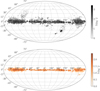 |
Fig. 1 Distribution in sky (Galactic coordinates) of sources of SDSS-V mwm_ob program observed until February 2025 (top, grey, 165 460 sources) and of the filtered sample described in Section 2.2 (bottom, orange, around 45 487 stars). The sources of the mwm_ob program are mostly located in the Galactic plane and the MCs. |
2.2 The hot-star sample
As mentioned above, the photometrically selected mwm_ob targets include a significant fraction of A-type stars and a modest fraction of cooler contaminants (see Sect. 2.3 in Z21). We therefore filtered the mwm_ob sample for the subsequent analysis to obtain a sample of hot stars with well-determined spectroscopic parameters and distances; we call this the hot-star sample (HSS). The filtering is based on four parameters: the signal-to-noise ratio of the observed single-epoch spectra, parallax error, renormalised unit weight error (RUWE; Lindegren 2021), and the effective temperature derived from the BOSS spectra.
Figure 2 shows a flow chart detailing the steps to construct the HSS. DR20 contains around a third of the target sample of the mwm_ob program. By the end of the survey, around 60% of the sources will have at least one observation. We note, however, that this is an estimate based on the theta-3 version of Robostrategy (Blanton et al. 2025). The survey strategy has slightly changed and the survey efficiency has improved, therefore the final numbers will be different.
We required the median signal-to-noise ratio (sn_median_all) of the single-epoch spectra in the BOSS pipeline summary file (reduction version v6_2_0, Morrison et al., in prep.) to be S/N>20, to ensure the reliability of the estimated spectral parameters. We selected sources with the parallax relative error σϖ/ϖ<0.2 and RUWE <1.4. The former cut aims to select sources with good distance determinations, and the latter seeks to remove sources with spurious parallaxes or proper motions (and possibly binaries, Belokurov et al. 2020).
We selected stars with Teff>10 000 K, according to the BOSS Net estimates (Sizemore et al. 2024). BOSS Net is a neural network that predicts self-consistent Teff and log g (with respective precision of 0.008 and 0.1 dex at S/N ∼ 15) in optical (BOSS and LAMOST) spectra for stars of all spectral types. For O-, B-, and A-type stars it was trained on LAMOST spectra with parameters determined by the HotPayne (Xiang et al. 2022). Additionally, it provides an independent estimate of stellar line-of-sight velocities (v_{l.o.s.,BNet}). Figure 3 shows a comparison of spectral parameters derived by BOSS Net (left Teff, centre log g) with those estimated by the Gaia ESP-HS pipeline. Both Teff and log g derived by the ESP-HS pipeline are on average higher than those provided by BOSS Net, but they broadly agree with one another. Around 70% and 80% of sources have parameters within 2 σ, for Teff and log g, respectively, which is sufficient for the purposes of this study. We refer to Villaseñor et al., (in prep.) for a thorough validation of the spectral parameters with synthetic spectra.
Figure 1 (bottom) shows the distribution in the sky of the HSS. The selection criteria of the HSS effectively select sources in the Galactic plane, excluding high-latitude sources and the Milky Clouds (MCs)2. The MC sources are mostly excluded by the requirement σϖ/ϖ<0.2. The HSS results in a sample of 99 494 spectra of 45 487 stars, with minimum and maximum distance, respectively, of 46 pc and 11 kpc, with average distance errors of ∼20, 70, 150, 300, and 500 pc at 1, 2, 3, 4, and 5 kpc. With respect to the D23 sample, the SDSS-V hot-star filtered sample covers a wider area of the Galactic plane. This is illustrated and further discussed in Appendix A.
Figure 4 shows the distribution of targets of the mwm_ob program passing the quality cuts described above (grey histogram) and the HSS (orange histogram) in the log Teff−log g diagram. The main contaminants of the mwm_ob program are A-type and F-type stars (33 309 and 4065 sources, respectively) that are difficult to separate from O- and B-type stars by using only Gaia and 2MASS photometry. There is also a small number of giants at log g ∼ 2.5 dex. These sources are likely included because they have the same colours in the G−Ks versus J−H colour–colour diagram as reddened O- and B-type stars (see Fig. 3 in Z21). Among the O- and B-type stars, 29 503 sources have temperature between 10 400 K and 17 000 K (spectral type between B9 and B3); 10 632 sources have temperatures between 17 000 K and 319 000 K (B3-O9.5); 213 sources have temperatures higher than 31 900 K (O9.5 and above), from which 131 are classified as O stars in SIMBAD.
We compared the HSS with the ALS-III catalogue (Pantaleoni González et al. 2025), which consists of a reliable sample of Galactic OB stars. We downloaded the ALS-III catalogue from the web interface3 (20 387 sources), and selected the sources flagged as “M”. This sample (14 273 sources) contains stars that are above the ZAMS and the 20 kK extinction track. In addition, these stars have Gaia DR3 photometry consistent with them being massive stars and have been reported as O- or B-type stars in the literature or have been spectroscopically validated. We cross-matched the ALS-III full and M sample with (1) the HSS; (2) the end of survey sample (theta-3 version of Robostrategy); (3) the target sample described in Z21 with the condition MK<−0.6 mag; and (4) the full target sample presented in Z21. We performed positional cross-matches, with a radius of 1”. Table 1 reports the results of the cross-matches.
The number of stars in common between the HSS and the ALS-III catalogues is currently relatively low (around 20% and 15% of the ALS-III M and full samples), but it will increase to around 50% (40%) of the ALS-III M (full) targets at the end of the survey. The initial target sample presented in Z21 contained around 87% (80%) of the ALS-III M (full) sample. Most of the ALS-III stars not included in the Z21 target sample have MK> −0.6 mag. Finally, the remaining 40 129 (40 083) sources in the HSS not included in the ALS-III M (full) sample include 130 O-type stars (Teff>31 900 K) and 8483 (8458 when comparing with the full sample) early B-type stars (Teff>17 000 K).
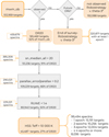 |
Fig. 2 Flowchart illustrating steps to construct HSS described in Sect. 2.2. The notation v.theta-3* indicates that the numbers are provisional and refer to the specific Robostrategy version named theta-3 (Blanton et al. 2025). The survey efficiency has improved, and the final number of observed targets will likely increase in the future. |
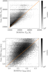 |
Fig. 3 Comparison between BOSS Net parameters and Gaia DR3 ESP-HS parameters for the hot-stars sample. The dashed orange lines correspond to the 1:1 relation. |
Cross-match with the ALS-III catalogue (Pantaleoni González et al. 2025).
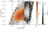 |
Fig. 4 Kiel diagram of sources in mwm_ob program (grey histogram) passing the quality cuts described in Section 2.2 and of those in the HSS (coloured histogram). The dashed vertical lines mark the following temperatures: 31 000 K (O9.5V type star), 17 000 (B3V type star), 10 400 K (B9V type star), 7400 K (A9V type star), and 6050 K (F9V type star). |
2.3 Line-of-sight velocities
To derive the 3D kinematic properties of our sample, we combined astrometric data from Gaia DR3 with SDSS-V’s line-of-sight velocities, vl.o.s.. In the SDSS-V context (Kollmeier et al. 2025; SDSS Collaboration 2025), there are two sets of estimates for line-of-sight velocities: those determined by the overall BOSS pipeline, vl.o.s.,XCSAO, and those determined by the BOSS Net method, vl.o.s.,BNet. The vl.o.s.,XCSAO were determined using the Python implementation of the cross-correlation technique first proposed by Tonry & Davis (1979), pyXCSAO (Kounkel 2022). pyXCSAO performs Fourier-based crosscorrelation between an observed spectrum and template Phoenix spectra (Husser et al. 2013). It also estimates the XCSAO_RVX parameter, which measures the strength of the correlation peak relative to the noise. In our analysis, we used vl.o.s.,XCSAO for stars with XCSAO_RVX > 6 (95% of the targets). Only if the strength of the correlation is lower than this boundary did we use vl.o.s.,BNet.
For targets with multi-epoch observations, we determine vl.o.s. as the average of the available epochs. We note that for most sources there are not enough epochs to compute orbital solutions and, therefore, the systemic velocity of binary systems that were not excluded by previous cuts. For single stars, this process improves the vl.o.s precision; for binaries (or multiples), the resulting vl.o.s. better approximates the centre of mass motion. We tested this method by simulating a population of stars with 50% binary fraction, observed at the same MJDs and with the same errors on line-of-sight velocities as our observed HSS. The results of these simulations are further discussed in Appendix C.
Line-of-sight velocity (vl.o.s.) uncertainties for single-epoch hot stars are typically ∼ 10 km/s (for both XCSAO and BOSS Net) and increase slightly with effective temperature. This trend arises because SDSS-V uses a fixed 15-minute exposure time for all sources, resulting in similar S/Ns. Further, at higher temperatures, the hydrogen lines that dominate the cross-correlation become broader, reducing velocity precision. For stars with a single observation, we adopted the uncertainty provided by XCSAO/BOSS Net; for stars with multiple observations, we calculated  .
.
To validate the vl.o.s estimates, we compared them with Gaia DR3 line-of-sight velocities (Fig. 5). As prescribed by Blomme et al. (2023), we applied the following correction to the Gaia DR3 vl.o.s. for OB stars:
 (3)
(3)
The subset of sources for which a Gaia DR3 vl.o.s. is available and reliable is relatively small (around 10% of the initial Gaia Collaboration (2023) query), and the cross-match with our sample is of 5959 single sources. The agreement between these estimates is satisfactory, with around 50% of the line-of-sight velocity in agreement within 1 σ and 75% in agreement within 2 σ. Outliers can be due to the use of the wrong spectral fitting template by the Gaia and or the XCSAO pipeline, or by strong line-of-sight velocity variations, for instance due to binarity.
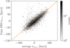 |
Fig. 5 Comparison between Gaia DR3 and SDSS-V XCSAO/Boss net line-of-sight velocities (in km/s). The orange dashed line corresponds to the 1:1 relation. |
 |
Fig. 6 Azimuthal velocity vφ as function of galactocentric radius, R. The histogram shows the azimuthal velocity distribution. The dashed orange lines indicate the boundaries of our selection: between 190 and 250 km/s. |
3 Streaming motions and age maps
In the previous section we constructed a well-defined sample of spectroscopically confirmed hot massive stars in the Milky Way disc (the HSS). In this section, we derive the kinematic properties and the ages of this sample. We present maps that can be constructed from it, focusing on the distribution of galactocentric radial velocities (Fig. 7) and ages (Fig. 8).
3.1 Deriving the 3D positions and kinematics
To compute stellar positions in Cartesian galactocentric coordinates X, Y, and Z we adopted the Sun’s galactocentric position (R, Z) = (8.2, 0.025) kpc (GRAVITY Collaboration 2019; Jurić et al. 2008) and galactocentric cylindrical velocities (.vR, vφ, vz)= (11., 232.24, 7.25) km/s (Schönrich et al. 2010), and photogeometric distances for each target (Bailer-Jones et al. 2021). To derive the radial, azimuthal, and vertical galactocentric velocities for each target and the associated uncertainties we followed the procedure described in D23 (see their Sections 3.2 and 3.3). The median galactocentric radial velocity uncertainty  is around 13 km/s for single sources, and around 8 km/s for sources with N ≥ 2 observations.
Figure 6 shows the azimuthal velocity vφ of the filtered sample as a function of galactocentric radius. Within R ≲ 5.5 kpc, we observe hints of non-axisymmetric dynamics due to the presence of the bar in the Milky Way. The over-densities in the data distribution reflect the selection function of the sample. For instance, the over-densities at R ∼ 10 kpc correspond to the density enhancement at X, Y ∼(−10, 2) shown in Fig. 7 (left). Whilst it is not the goal of this paper to fit the rotation curve, we used the fact that stars belonging to the HSS follow cold circular orbits to remove outliers. More precisely, we removed stars whose vφ’s are not between 190 km/s and 250 km/s (orange dashed lines in Fig. 6). This removes around 5000 objects whose velocities do not closely follow galactic rotation, either due to an erroneous estimate of the radial-velocity solution or because they are characterised by peculiar motions deviating from the average azimuthal velocity. These stars in turn could be binaries that have not been filtered out from the sample with the RUWE cut or runaway stars (Hoogerwerf et al. 2001), for example. A detailed analysis of this population is left for future work.
Figure 7 (left) shows the density distribution of the HSS in the Galactic plane. The map is computed by dividing the Galactic plane into spatial bins (spaxels) of a constant size of 250 × 250 pc. We note that while some of the over-densities in the spatial distribution of the HSS do correspond to young associations and clusters, the overall appearance of the in-plane distribution is driven by the survey selection function. For instance, the lack of sources at negative X values and Y between 0 and 2 kpc is due to a lack of observations at −180 ≲ l ≲−160 (see Fig. 1). This is partly because the survey is still ongoing, and some regions of the sky have not yet been observed. Conversely, other fields have been observed more frequently due to the survey observing strategy, which includes repeated visits to selected areas; as a result, these fields contain a higher number of observed targets.
We estimated the average galactocentric radial velocity, v̄R, in each spaxel and its associated dispersion, σR, by optimising the log-likelihood of the distribution of observed velocities vR, i (with uncertainties σvR, i of the stars located within the jt h-spaxel). We assumed Gaussian uncertainties, so the negative log-likelihood to minimise is
 (4)
(4)
We considered only the spaxels with >5 stars. Figure 7 (right) shows the distribution of the HSS colour-coded by v̄R. Figure B.1 shows the velocity dispersion σR of the sample. In Fig. 7, stars moving on average towards the Galactic centre are coloured in blue, whereas outwards-moving stars are coloured in red. Radial motions within the solar circle (between the Sun and the Galactic centre) are predominantly directed inwards (negative galactocentric radial velocities). Radial motions outside the solar circle (R ≳ 8 kpc) are instead predominantly directed outwards (positive galactocentric radial velocities). The inward motions show strong asymmetric signatures. These features extend over several kiloparsecs, with the most prominent drawing an arc-like segment almost extending over the entire reach of the sample. We further discuss this result in Section 4.
3.2 Ages
We estimated the ages of the HSS members following the methodology proposed by Jørgensen & Lindegren (2005, JL05) and, more recently, Howes et al. (2019) and Sahlholdt & Lindegren (2021). Using the same notation as JL05, we wrote the posterior probability f(τ, Z, m) for the log-age τ, metallicity Z, and mass m, as
 (5)
(5)
where f0(τ, Z, m) is the prior on log-age, mass, and metallicity, and ℒ(t, Z, m) is the likelihood function. Integrating with respect to m and Z gives f(τ), the posterior pdf of τ, which summarises the available information concerning the log-age of the star.
We wrote the prior f0(τ, Z, m) as the product of three independent components:
 (6)
(6)
We chose a uniform prior in age t, ψ(t)=c; therefore, as probability densities need to be conserved,
 (7)
(7)
with τ=log10 (t). For simplicity, we set c̃=1. The prior on the metallicity, Z, or, more precisely, on the iron abundance [Fe/H], is given by a Gaussian distribution centred around the mean metallicity at a given galactocentric radius:
 (8)
(8)
We determined the mean Zexp=Zexp(RGal) using the relation found by Hackshaw et al. (2024):
 (9)
(9)
and we assumed a constant σZ=0.1 dex. Finally, we assumed a simple power law for the stellar mass prior:
 (10)
(10)
where α=−2.7, which is representative for the empirical IMF at m>1 M⊙ (Kroupa 2002).
For each star, we adopted a set of observables – effective temperature (Teff), surface gravity (logg), and absolute magnitude in the K band (MK) – and compute the likelihood assuming Gaussian uncertainties on these parameters:
 (11)
(11)
where d = (Teff, log g, MK) are the observed values with uncertainties, σi, and qi(τ, Z, m) are the corresponding model predictions for age, τ, mass, m, and metallicity, Z, interpolated from stellar isochrones.
Integrating over m and Z, the posterior probability of log-age τ can be written as
 (12)
(12)
where
 (13)
(13)
In practice, we approximated the integral over mass m and Z as
 (14)
(14)
where mi j k are the initial-mass values along each isochrone (τk,.Zj). Finally, we multiplied the marginalised likelihood by the prior on the log-age, ψ(τ), and normalised the posterior distribution. We evaluated f(τ) using MIST (Choi et al. 2016; Dotter 2016, MIST version 1.2, with initial v/v_crit = 0.4) isochrones equally spaced (0.05 dex) by log age from 1 Myr to 1 Gyr and with [Fe/H] from −0.5 to +0.4 dex, in steps of 0.1 dex. We used the 50 th percentile of f(τ) as our age estimator, and the semidifference between the 84th and 16th percentiles of f(τ) as our uncertainty estimator.
Figure 8 shows a map of mean ages in the Galactic plane in spaxels of 125 × 125 pc. Only spaxels with more than five stars are shown. Wide clumps of stars with young ages (log-age ≲ 7.5 ∼ 30 Myr) are visible. These correspond to star formation regions and are further discussed in Section 4. 85% of the HSS is younger than ∼ 320 Myr (log-age = 8.5 dex). The median age uncertainty of the entire sample is 15 Myr. For stars younger than 30 Myr (log-age = 7.5), the median age uncertainty is ∼ 4 Myr, for stars older than ∼ 150 Myr (log-age = 8.2) is ∼ 30 Myr.
We validated our age estimates by comparing with the age estimates for clusters provided by Hunt & Reffert (2023, H23;) and Cantat-Gaudin et al. (2020, CG20). We cross-matched our HSS with the cluster members of both H23 and CG20 (with membership probability >50% and 90%, respectively), we evaluated the posterior distributions f*(τ) of the hot-star (HS) cluster members and multiplied them together (under the reasonable assumption that cluster members are coeval) and computed the HS cluster age as the 50th percentile of the total posterior distribution, fHS=∏* f*(τ). We only used clusters with at least five HSs with posteriors narrower than 0.3 dex in log-age (which is around a factor of 2 on age). Figure 9 shows the comparison between the HS cluster ages and H23 (left) and CG20 (right). The comparison with H 23 and CG20 is satisfactory. With respect to CG20, our ages seem to be slightly over-estimated (although CG20 does not provide errors on their age estimates). With respect to H23 they agree well, except for a few outliers. The uncertainties of age estimates are much smaller than those estimated by H23: this might mean that our method tends to underestimate uncertainties. In any case, the ages determined in this work are intended as youth indicators rather than exact age determinations.
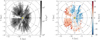 |
Fig. 7 Distribution of hot-star sample in Galactic plane. The left panel shows the density distribution of the sources. The right panel shows the distribution of sources colour-coded by their galactocentric radial velocity (computed as described in the text). In both panels, the Sun is in X, Y=(−8.2, 0) kpc, and it is indicated by the yellow star. The Galactic centre is in X, Y = (0, 0) kpc. The dashed circles have radii of 2, 4, 6, 8, and 10 kpc. The solid lines indicate constant Galactic longitudes. |
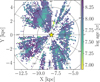 |
Fig. 8 Mean log-age map of hot-star sample in the Galactic plane. The mean ages are computed only for spaxels with more than five stars. The dashed circles have radii of 2, 4, and 6 kpc. The yellow star indicates the Sun’s position. The solid lines indicate constant Galactic longitudes. |
4 Discussion
Figure 7 (right panel) shows that massive young stars in the Milky Way disc have remarkably strong radial motions that are coherent over several kpc. These large-scale kinematic patterns in the X−Y plane could be a signature of the dynamical response of young massive stars to the Milky Way’s spiral structure, but could also arise from other phenomena, such as the influence of the bar, resonant interaction, or incomplete phase mixing following some perturbation. In this section, we put our results in the context of several observational studies and simulations and compared the motions of younger and older sources.
4.1 Comparison with spiral-arm tracers
Figure 10 shows a comparison between the v̄R map and the density distribution of the OB star sample of Zari et al. (2021) and the spiral-arm models derived by Reid et al. (2019). The left panel of Fig. 10 shows the density contrast of the OB sample, defined as
 (15)
(15)
We computed ΔΣ using a similar procedure to Poggio et al. (2021). We derived the 3D density ρ(X, Y, Z) of the OB sample by smoothing the spatial distribution of stars with a 3D Gaussian filter with a bandwidth of w=10 pc and an average density of  by smoothing with a larger bandwidth of w=100 pc. We truncated both filters at 3 σ. We projected the distribution on the Galactic plane by integrating over Z to derive Σ=Σ(X, Y) and
  ; finally, we computed ΔΣ. The OB-star over-densities are interpreted as spiral-arm segments. Surprisingly, the middle panel of Fig. 10 shows that the kinematic structures are not aligned with the OB star density. The black lines in right panel of Fig. 10 show the spiral-arm model derived by Reid et al. (2019). While the alignment is not perfect, the model seems to follow the kinematic structure slightly more closely.
Figure 11 shows the density distribution of young (≤ 30 Myr, left, 7704 stars) and older (≳ 150 Myr, right, 12 169 stars) stars in our sample. The solid lines correspond to the Δ Σ contours computed with Eq. (15) and showed in Fig. 10. The young star distribution is clustered, and shows several clumps that can be associated with OB associations and star formation complexes, such as those towards Cygnus (Wright et al. 2016; Berlanas et al. 2020), Cassiopeia (W3, W4, W5, Gouliermis et al. 2014), Carina (Tr14, Tr15, Tr16, Berlanas et al. 2023), and Sagittarius and Serpens (M20, M17, Povich et al. 2007; Kuhn et al. 2021). The density distribution of the youngest sources traces the density enhancements of the overall OB star distribution (consistent with Fig. 4 of Zari et al. 2023). The older stars (>150 Myr) show less prominent density variations. The residual over-densities might be artefacts due to uncertainties in the age estimates and to the survey selection function (i.e. in some fields more targets are observed than in others), or they might still reflect spiral structure (see Zari et al. 2023).
While a connection between spiral arms and the kinematics of nearby stars and gas is expected, establishing a direct link is not straightforward. The youngest stars, formed within spiral arms, are expected to inherit the motions of their parent molecular clouds, which typically rotate with relatively low random velocities. The bulk motion of star-forming gas within spiral arms is influenced by shear arising from gravitational torques. In the reference frame of the spiral pattern, gas located on the trailing side of the arm moves outward, while gas on the leading side moves inward (see, e.g. Kawata et al. 2014). If shocks are present along the leading edge of the spiral arms, raising gas pressure, this may lead to enhanced star formation in these regions (Meidt et al. 2013). Consequently, stars formed on the leading side are expected to be more numerous and to exhibit a net negative radial velocity. The amplitude of the radial-velocity component of newly formed stars depends on both the spiral pattern speed and the pitch angle. Therefore, the observed mean negative radial velocities inside galactocentric radii of <9 kpc (as shown in Figs. 7 and 10) suggests that a significant fraction of these stars formed in spiral arms and still retain the bulk motion of their natal gas. This idea is also supported by recent studies of young stellar clusters (Swiggum et al. 2025), which showed that clusters formed near spiral arms exhibit systematic radial motions that might track the passage of the arm and the associated gas compression.
The observed spatial offset between spiral arms traced by maser sources (Reid et al. 2014, 2019) and those traced by young stars can be attributed to differences in the orbital frequencies of stars formed at various locations along the spiral arms, relative to the pattern’s corotation. In the case of rigidly rotating spiral patterns, this results in the youngest stars being located within the spiral arms, while somewhat older stars (∼100 Myr) appear downstream in the inter-arm regions (Dobbs & Pringle 2010). While this picture is intuitively appealing, it breaks down for tidally induced or flocculent spiral structures, where a clear age gradient is not expected. Although one could, in principle, model the displacement of stars as a function of their age, such an approach requires assumptions about the historical structure, kinematics, and the origin of the Milky Way spiral arms, an analysis that lies beyond the scope of the present study.
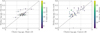 |
Fig. 9 Comparison between ages for clusters determined in this work and by Hunt & Reffert (2023) and Cantat-Gaudin et al. (2020). The colour bar represents the number of hot stars in the cluster. The dashed line represents the 1: 1 relation in both panels. |
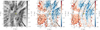 |
Fig. 10 Comparison between density distribution of OB stars, the spiral-arm model from Reid et al. (2019), and the radial velocity asymmetries. In the left panel and central panels, the solid black contours represent the 0 and 0.5 density-contrast levels. In the right panel, the spiral arms are named following Reid et al. (2019): Outer Arm; Perseus Arm; Local Arm; Sagittarius-Carina Arm; Scutum-Centaurus Arm. In the three panels, the yellow star indicates the Sun’s position in X, Y=−8.2, 0 kpc, and the Galactic centre is located in X, Y = 0, 0 kpc. The dashed lines represent circle radii of 2, 4, and 6 kpc. The solid lines indicate constant Galactic longitudes. |
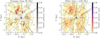 |
Fig. 11 Density distribution of young (<30 Myr; left) and older (>150 Myr) sources. In the left panel, star forming regions are indicated. The solid contour lines represent the density distribution of all sources (Fig. 10, left) and are computed as described in Sect. 4. The labels highlight some of the more prominent OB associations (their locations are from Table 1 of Wright 2020). The solid lines indicate constant Galactic longitudes. |
4.2 Comparison with Aurigaia
To gain better insights into our results, we compared our observational data with the mock stellar catalogues generated from the AURIGA cosmological simulations (Grand et al. 2018)4. Here, we show the HITS mocks catalogue generated using the SNAP-DRAGONS code by Hunt et al. (2015) with the following parameters: Halo 6, resolution level 3, extinction; however, we found analogous results by using all the available HITS mock catalogues (Halo 16, 21, 23, 24, and 27). The angle between the Sun and the Galactic-centre line and the major axis of the bar is 30 deg. We used the following ADQL script to replicate the HSS selection function:
Gmagnitude < 16.0 mag
Age < 0.5 Gyr
EffectiveTemperature > 10 000 K.
Figure 12 (top left) shows the density distribution of the sources we selected. The aurigaia catalogue is limited to V<16 mag; therefore, the coverage of the Galactic plane is very similar to our observed sample. The density distribution traces the spiral structure of the simulated galaxy, with visible over-densities corresponding to segments of spiral arms. Figure 12 (top right) shows the same distribution, colour-coded by galactocentric radial velocities. The simulation shows radial-velocity asymmetries, with comparable amplitude to those shown in Fig. 7. The bi-symmetric feature on either side of the Galactic centre, with negative and positive values on each side of the apparent major axis of the bar, is generated by the Galactic bar. The qualitative agreement between our data and the aurigaia simulation suggests that radial-velocity asymmetries are a common feature in spiral galaxies. There are, however, a few differences. In the simulation, the stellar over-densities within ∼ 6 kpc of the Sun have coherent outwards motions, while the stellar over-density at R ∼ 6−8 kpc towards the outer Galaxy exhibits mostly inwards motions. In our observations instead, stars seem to be moving mostly towards the Galactic centre, and only a few stellar overdensities move outwards (such as those at X<−10, Y<0 kpc). These discrepancies might depend on the detailed properties of spiral arms in the simulations (position, pattern speed, etc.). Even in the simulation, the spiral-arm segments do not all move at constant speed, with over-densities moving with both positive and negative velocities.
4.3 Comparison with kinematic studies
We now compare our results with two observational studies based on young stars: D23; Poggio et al. (2025, P25). D23 found that the velocity field of the OB stars shows streaming motions that have a characteristic length similar to the spiral-arm density. The region sampled by the OB sample in D23 extends up to distances of ∼ 2 kpc; thus, the streaming motions in the OB stars mainly map the Local Arm. Conversely, the sample that we used in this study is highly incomplete at distances below 2 kpc. This is due to both the selection function of the sample (see Z21) and the observing strategy (Medan et al. 2025). However, our sample extends even beyond 6 kpc towards certain lines of sight, allowing us to map the velocities of HSs at a much larger volume than D23. Thus, comparing the two samples in the same volume is – at the moment – almost impossible. As a sanity check, we verified that the stars in common between the two samples have comparable vR (see also Section 2). P25 studied the median galactocentric radial velocity for a sample of young giants (age ≲ 100 Myr) and Cepheids and found a strong feature in the v̄R velocity field. They interpreted this feature as the signature of a wave propagating towards the outer disc and suggested that the kinematics of young stars in the outer disc is dominated by this outwards motion. Figure 7 shows that towards the outer disc, at distances larger than ∼ 2 kpc from the Sun, the radial motions of the HSS are directed outwards; this is similar to P25, albeit with stronger v̄R variations (−30<v̄R<30 km/s as compared to −15<v̄R<15 km/s found by P25). Towards the inner disc, we detect stronger inwards motions than those reported by P25. This is likely due to the differences in the samples used in the two studies. For instance, the spatial distribution of the young giant sample in Fig. 4 of P25 presents different features than the one shown in Fig. 7.
Another key question is how to relate the motions and orbits of young and old sources. Figure 13 shows an updated version of Fig. 1 in Eilers et al. (2020), which was generated using APOGEE DR17 RGB stars selected as detailed in Appendix D. Eilers et al. (2020) interpreted the v̄R feature visible in Fig. 13 as the kinematic signature of a logarithmic spiral arm. This feature differs morphologically from that in Fig. 7. Towards the Galactic centre, at RGC ≲ 8 kpc the RGB sample shows positive v̄R, while the HSS shows negative radial velocities. Moreover, the amplitude of the radial-velocity asymmetries is lower by a factor of about three. Instead, some similarities are visible towards the outer Galaxy. For instance, in the region corresponding to the Perseus Arm – between 2 and 4 kpc and Y > 0 kpc from the Sun > both samples show negative radial velocities, while for Y<0 kpc, the velocities switch to positive values. Similar to the observed data, the radial-velocity distribution of the young and old populations in the aurigaia mock data set is markedly different. Figure 12 (bottom) shows the density distribution (left) and radial velocities (right) of a population of giant stars extracted from the aurigaia catalogue using the same selection criteria described in Appendix D. The giant star population displays (a) a quadrupole feature associated with the Galactic bar, and (b) alternating inward and outward motions across the disc. While these motions are stronger than those observed in the data (Fig. 13), the alternating pattern of positive and negative velocities is qualitatively similar. The strength of the stellar response to spiral perturbations is expected to diminish with age. This attenuation arises from the increase in stellar velocity dispersion over time, which reduces the effectiveness of spiral arms in influencing older populations. As a result, a mixed stellar population responds differentially to the same spiral structure, depending on age and kinematic heating. This phenomenon, known as kinematic fractionation, was originally proposed to explain the vertical structure of X-shaped bulges (Debattista et al. 2017), but similar dynamics are at play across spiral arms as well (Khoperskov et al. 2018). This mechanism accounts for observed variations in stellar metallicity across spiral arms (e.g. Poggio et al. 2022; Hawkins 2023; Hackshaw et al. 2024), and it naturally explains the structure observed in the kinematic maps of young and old stellar populations in the data and in the aurigaia mock data. Thus, young stars, though not necessarily formed within the prominent spiral arms, exhibit a stronger response to the spiral structure – as evidenced by their larger radial velocity amplitudes (v̄R) – in contrast to the smoother, more featureless kinematics of older stars.
In general, spiral arms introduce small-scale radial-velocity perturbations that are superimposed on the large-scale radial-velocity pattern induced by the Milky Way bar. While the characteristic quadrupole pattern associated with the bar’s influence inside its corotation radius (<5-−6 kpc; see e.g. D23) is largely absent in Figs. 7 and 10 (and similarly in the mock Auriga simulation; see Fig. 12, top), the bar also generates non-circular motions at larger radii. The disc’s response to the spiral structure and the Galactic bar has been explored by Khoperskov et al. (2024) and Monari et al. (2016a,b, M16a, M16b). M16a found that stars located on the arms tend to move inward (v̄R<0), while stars in the inter−arm regions move outward (v̄R>0). M16b confirmed these findings and additionally showed that the Galactic bar dominates the horizontal motions (vR and v φ). These results are in qualitative agreement with the features seen in Fig. 13 (cf. Fig. 1 in Monari et al. (2016a) and Figs. 4–8 in Monari et al. (2016b), but they do not reproduce the v̄R features shown in Fig. 7 for the HSS. To isolate the localised radial-velocity perturbations introduced by spiral arms, it is necessary to subtract the bar-induced bulk motion. This subtraction, however, requires assumptions regarding the 3D mass distribution of the bar and its pattern speed.
Modelling the response of populations of different ages to the spiral arm potential or to other perturbations is beyond the scope of this paper, and will be the focus of future works. The important point, at present, is that old and young stars exhibit remarkably different kinematic patterns, particularly within the solar circle, both in real and simulated data. These patterns are likely due to the effects on young stars of the spiral structure and the bar of our Galaxy.
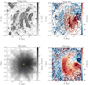 |
Fig. 12 Density distribution (left) and galactocentric radial velocities (right) of the gaiauriga mock stellar catalogue for young (top) and old (bottom) sources. The black lines outline the contours of the density distribution. The black dot indicates the Galactic centre, the yellow star the Sun’s position. The dashed black lines mark concentric circles at ΔR = 2 kpc. The v̄R> feature for R ≲ 5 kpc in the right panels is due to the effect of the bar on the kinematics of sources in the inner galaxy. The solid lines indicate constant Galactic longitudes. |
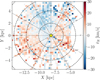 |
Fig. 13 Distribution of red giant stars in Milky Way disc from APOGEE DR17. The red giant stars are colour-coded by their average galactocentric radial velocity. The location of the Sun is indicated by the yellow star. The dashed black lines mark concentric circles at ΔR = 2 kpc. The solid lines indicate constant Galactic longitudes. The region within 5 kpc of the Galactic centre is masked as the stellar motions in that region are influenced by the bar. |
5 Summary and conclusions
In this study, we present the first kinematic analysis of young OB stars in the Milky Way disc based on BOSS spectroscopic observations from SDSS-V, combined with astrometry from Gaia DR3. We constructed a sample of spectroscopically confirmed hot stars (HSS; Teff>10 000 K) with reliable radial velocities and distances, covering almost the entire Galactic plane and extending to distances up to ∼ 5 kpc from the Sun.
We derived the 3D motions of this sample, and we studied the distribution on the X−Y plane of galactocentric radial velocities, v̄R. The HSS exhibit large-scale features in vR, with amplitudes reaching ± 30 km s−1. These velocity structures are spatially coherent over kiloparsec scales.
We estimated the ages of all sources in the HSS with a Bayesian isochrone fitting procedure. These age estimates provide an indication of the youth of the sources more than an exact estimate. While the distribution of sources younger than 30 Myr closely follows the density enhancements of the entire sample, the observed kinematic patterns are not straightforwardly aligned with known spiral arms, and are not associated only with the young (<30 Myr) or older sources (>150 Myr).
We compared our results with mock catalogues generated from the AURIGA cosmological simulations (Grand et al. 2018) and with other observational studies based on different stellar samples. The radial velocity features observed in the data are observed in simulations as well, for sources younger than 500 Myr. Most of the observational studies that focus on the kinematics of the disc use samples of older sources. It is therefore not surprising that the features observed in the v̄R distribution in the X−Y plane (e.g. Eilers et al. 2020) for older sources, such as RGB stars, show different properties compared to those we observe in our sample.
A plausible interpretation of the observed kinematic structures in the young stellar population is that they reflect a superposition of the effect of the Milky Way bar and spiral arms. A more detailed analysis and modelling is left for future work. This will require a more complete sample (SDSS-V will continue observations until 2027, and the current data set amounts to around a third of the anticipated survey sample) and a model of Galactic structure and dynamics including populations of different ages.
Acknowledgements
We thank the referee for their constructive comments that helped improve the quality of this manuscript. Funding for the Sloan Digital Sky Survey V has been provided by the Alfred P. Sloan Foundation, the HeisingSimons Foundation, the National Science Foundation, and the Participating Institutions. SDSS acknowledges support and resources from the Center for HighPerformance Computing at the University of Utah. SDSS telescopes are located at Apache Point Observatory, funded by the Astrophysical Research Consortium and operated by New Mexico State University, and at Las Campanas Observatory, operated by the Carnegie Institution for Science. The SDSS web site is www.sdss.org. SDSS is managed by the Astrophysical Research Consortium for the Participating Institutions of the SDSS Collaboration, including the Carnegie Institution for Science, Chilean National Time Allocation Committee (CNTAC) ratified researchers, Caltech, the Gotham Participation Group, Harvard University, Heidelberg University, The Flatiron Institute, The Johns Hopkins University, L’Ecole polytechnique fédérale de Lausanne (EPFL), Leibniz-Institut für Astrophysik Potsdam (AIP), Max-Planck-Institut für Astronomie (MPIA Heidelberg), Max-Planck-Institut für Extraterrestrische Physik (MPE), Nanjing University, National Astronomical Observatories of China (NAOC), New Mexico State University, The Ohio State University, Pennsylvania State University, Smithsonian Astrophysical Observatory, Space Telescope Science Institute (STScI), the Stellar Astrophysics Participation Group, Universidad Nacional Autónoma de México, University of Arizona, University of Colorado Boulder, University of Illinois at Urbana-Champaign, University of Toronto, University of Utah, University of Virginia, Yale University, and Yunnan University. The research leading to these results has (partially) received funding from the Research Foundation Flanders (FWO) under grant agreement G089422N, as well as from the BELgian federal Science Policy Office (BELSPO) through the PRODEX grant for PLATO. This work has made use of data from the European Space Agency (ESA) mission Gaia (https://www.cosmos.esa.int/gaia), processed by the Gaia Data Processing and Analysis Consortium (DPAC, https://www.cosmos.esa.int/web/gaia/dpac/consortium). Funding for the DPAC has been provided by national institutions, in particular the institutions participating in the Gaia Multilateral Agreement. Software: Astropy, (Astropy Collaboration 2013, 2018, 2022), matplotlib (Hunter 2007), numpy (Harris et al. 2020), scipy (Virtanen et al. 2020), topcat (Taylor 2005).
References
- Almeida, A., Anderson, S. F., Argudo-Fernández, M., et al. 2023, ApJS, 267, 44 [NASA ADS] [CrossRef] [Google Scholar]
- Antoja, T., Helmi, A., Romero-Gómez, M., et al. 2018, Nature, 561, 360 [Google Scholar]
- Ardèvol, J., Monguió, M., Figueras, F., Romero-Gómez, M., & Carrasco, J. M., 2023, A&A, 678, A111 [NASA ADS] [CrossRef] [EDP Sciences] [Google Scholar]
- Astropy Collaboration (Robitaille, T. P., et al.,) 2013, A&A, 558, A33 [NASA ADS] [CrossRef] [EDP Sciences] [Google Scholar]
- Astropy Collaboration (Price-Whelan, A. M., et al.,) 2018, AJ, 156, 123 [Google Scholar]
- Astropy Collaboration (Price-Whelan, A. M., et al.,) 2022, ApJ, 935, 167 [NASA ADS] [CrossRef] [Google Scholar]
- Bailer-Jones, C. A. L., Rybizki, J., Fouesneau, M., Demleitner, M., & Andrae, R., 2021, AJ, 161, 147 [Google Scholar]
- Belokurov, V., Penoyre, Z., Oh, S., et al. 2020, MNRAS, 496, 1922 [Google Scholar]
- Bennett, M., & Bovy, J., 2019, MNRAS, 482, 1417 [NASA ADS] [CrossRef] [Google Scholar]
- Berlanas, S. R., Herrero, A., Comerón, F., et al. 2020, A&A, 642, A168 [NASA ADS] [CrossRef] [EDP Sciences] [Google Scholar]
- Berlanas, S. R., Maíz Apellániz, J., Herrero, A., et al. 2023, A&A, 671, A20 [NASA ADS] [CrossRef] [EDP Sciences] [Google Scholar]
- Blanton, M. R., Carlberg, J. K., Dwelly, T., et al. 2025, arXiv e-prints [arXiv:2505.21328] [Google Scholar]
- Blomme, R., Frémat, Y., Sartoretti, P., et al. 2023, A&A, 674, A7 [NASA ADS] [CrossRef] [EDP Sciences] [Google Scholar]
- Bowen, I. S., & Vaughan, A. H., J. Appl. Opt., 1973, 12, 1430 [Google Scholar]
- Cantat-Gaudin, T., Anders, F., Castro-Ginard, A., et al. 2020, A&A, 640, A1 [NASA ADS] [CrossRef] [EDP Sciences] [Google Scholar]
- Choi, J., Dotter, A., Conroy, C., et al. 2016, ApJ, 823, 102 [Google Scholar]
- Creevey, O. L., Sordo, R., Pailler, F., et al. 2023, A&A, 674, A26 [NASA ADS] [CrossRef] [EDP Sciences] [Google Scholar]
- de los Reyes, M. 2023, Phys. Online J., 16, 152 [Google Scholar]
- Debattista, V. P., Ness, M., Gonzalez, O. A., et al. 2017, MNRAS, 469, 1587 [Google Scholar]
- Dobbs, C. L., & Pringle, J. E., 2010, MNRAS, 409, 396 [NASA ADS] [CrossRef] [Google Scholar]
- Dotter, A., 2016, ApJS, 222, 8 [Google Scholar]
- Eilers, A.-C., Hogg, D. W., Rix, H.-W., et al. 2020, ApJ, 900, 186 [Google Scholar]
- Fouesneau, M., Frémat, Y., Andrae, R., et al. 2023, A&A, 674, A28 [NASA ADS] [CrossRef] [EDP Sciences] [Google Scholar]
- Frankel, N., Rix, H.-W., Ting, Y.-S., Ness, M., & Hogg, D. W., 2018, ApJ, 865, 96 [NASA ADS] [CrossRef] [Google Scholar]
- Gaia Collaboration (Brown, A. G. A., et al.,) 2021, A&A, 649, A1 [NASA ADS] [CrossRef] [EDP Sciences] [Google Scholar]
- Gaia Collaboration (Drimmel, R., et al.,) 2023, A&A, 674, A37 [CrossRef] [EDP Sciences] [Google Scholar]
- García Pérez, A. E., Allende Prieto, C., Holtzman, J. A.,, et al. 2016, AJ, 151, 144 [Google Scholar]
- Ge, Q. A., Li, J. J., Hao, C. J., et al. 2024, AJ, 168, 25 [NASA ADS] [CrossRef] [Google Scholar]
- Gouliermis, D. A., Hony, S., & Klessen, R. S., 2014, MNRAS, 439, 3775 [NASA ADS] [CrossRef] [Google Scholar]
- Grand, R. J. J., Helly, J., Fattahi, A., et al. 2018, MNRAS, 481, 1726 [Google Scholar]
- GRAVITY Collaboration (Abuter, R., et al.) 2019, A&A, 625, L10 [NASA ADS] [CrossRef] [EDP Sciences] [Google Scholar]
- Gunn, J. E., Siegmund, W. A., Mannery, E. J., et al. 2006, AJ, 131, 2332 [NASA ADS] [CrossRef] [Google Scholar]
- Hackshaw, Z., Hawkins, K., Filion, C., et al. 2024, ApJ, 977, 143 [Google Scholar]
- Harris, C. R., Millman, K. J., van der Walt, S. J., et al. 2020, Nature, 585, 357 [NASA ADS] [CrossRef] [Google Scholar]
- Hawkins, K., 2023, MNRAS, 525, 3318 [NASA ADS] [CrossRef] [Google Scholar]
- Hoogerwerf, R., de Bruijne, J. H. J., & de Zeeuw, P. T., 2001, A&A, 365, 49 [NASA ADS] [CrossRef] [EDP Sciences] [Google Scholar]
- Howes, L. M., Lindegren, L., Feltzing, S., Church, R. P., & Bensby, T., 2019, A&A, 622, A27 [NASA ADS] [CrossRef] [EDP Sciences] [Google Scholar]
- Hunt, E. L., & Reffert, S., 2023, A&A, 673, A114 [NASA ADS] [CrossRef] [EDP Sciences] [Google Scholar]
- Hunt, J. A. S., Kawata, D., Grand, R. J. J., et al. 2015, MNRAS, 450, 2132 [Google Scholar]
- Hunter, J. D., 2007, Comput. Sci. Eng., 9, 90 [NASA ADS] [CrossRef] [Google Scholar]
- Husser, T. O., Wende-von Berg, S., Dreizler, S., et al. 2013, A&A, 553, A6 [NASA ADS] [CrossRef] [EDP Sciences] [Google Scholar]
- Jørgensen, B. R., & Lindegren, L., 2005, A&A, 436, 127 [Google Scholar]
- Jurić, M., Ivezić, Ž., Brooks, A.,, et al. 2008, ApJ, 673, 864 [Google Scholar]
- Kawata, D., Hunt, J. A. S., Grand, R. J. J., Pasetto, S., & Cropper, M., 2014, MNRAS, 443, 2757 [NASA ADS] [CrossRef] [Google Scholar]
- Khoperskov, S., Di Matteo, P., Haywood, M., & Combes, F., 2018, A&A, 611, L2 [NASA ADS] [CrossRef] [EDP Sciences] [Google Scholar]
- Khoperskov, S., Minchev, I., Steinmetz, M., et al. 2024, MNRAS, 533, 3975 [CrossRef] [Google Scholar]
- Kollmeier, J. A., Zasowski, G., Rix, H.-W., et al. 2017, arXiv e-prints [arXiv:1711.03234] [Google Scholar]
- Kollmeier, J. A., Rix, H.-W., Aerts, C., et al. 2025, arXiv e-prints [arXiv:2507.06989] [Google Scholar]
- Kounkel, M., 2022, PyXCSAO [Google Scholar]
- Kroupa, P., 2002, Science, 295, 82 [Google Scholar]
- Kuhn, M. A., Benjamin, R. A., Zucker, C., et al. 2021, A&A, 651, L10 [NASA ADS] [CrossRef] [EDP Sciences] [Google Scholar]
- Leung, H. W., & Bovy, J., 2019a, MNRAS, 483, 3255 [Google Scholar]
- Leung, H. W., & Bovy, J., 2019b, MNRAS, 489, 2079 [Google Scholar]
- Lin, Z., Xu, Y., Hou, L., et al. 2022, ApJ, 931, 72 [NASA ADS] [CrossRef] [Google Scholar]
- Mackereth, J. T., Bovy, J., Leung, H. W., et al. 2019, MNRAS, 489, 176 [Google Scholar]
- Medan, I., Dwelly, T., Covey, K. R., et al. 2025, arXiv e-prints [arXiv:2506.15475] [Google Scholar]
- Meidt, S. E., Schinnerer, E., García-Burillo, S., et al. 2013, ApJ, 779, 45 [NASA ADS] [CrossRef] [Google Scholar]
- Monari, G., Famaey, B., & Siebert, A., 2016a, MNRAS, 457, 2569 [Google Scholar]
- Monari, G., Famaey, B., Siebert, A., et al. 2016b, MNRAS, 461, 3835 [Google Scholar]
- Montalbán, J., Mackereth, J. T., Miglio, A., et al. 2021, Nat. Astron., 5, 640 [Google Scholar]
- Palicio, P. A., Recio-Blanco, A., Poggio, E., et al. 2023, A&A, 670, L7 [NASA ADS] [CrossRef] [EDP Sciences] [Google Scholar]
- Pantaleoni González, M., Maíz Apellániz, J., Barbá, R. H., et al. 2025, MNRAS, 543, 63 [Google Scholar]
- Pecaut, M. J., & Mamajek, E. E., 2013, ApJS, 208, 9 [Google Scholar]
- Poggio, E., Drimmel, R., Cantat-Gaudin, T., et al. 2021, A&A, 651, A104 [NASA ADS] [CrossRef] [EDP Sciences] [Google Scholar]
- Poggio, E., Recio-Blanco, A., Palicio, P. A., et al. 2022, A&A, 666, L4 [NASA ADS] [CrossRef] [EDP Sciences] [Google Scholar]
- Poggio, E., Khanna, S., Drimmel, R., et al. 2025, A&A, 699, A199 [NASA ADS] [CrossRef] [EDP Sciences] [Google Scholar]
- Povich, M. S., Stone, J. M., Churchwell, E., et al. 2007, ApJ, 660, 346 [Google Scholar]
- Price-Whelan, A. M., 2017, J. Open Source Softw., 2, 388 [Google Scholar]
- Reid, M. J., Menten, K. M., Brunthaler, A., et al. 2014, ApJ, 783, 130 [Google Scholar]
- Reid, M. J., Menten, K. M., Brunthaler, A., et al. 2019, ApJ, 885, 131 [Google Scholar]
- Sahlholdt, C. L., & Lindegren, L., 2021, MNRAS, 502, 845 [CrossRef] [Google Scholar]
- Schönrich, R., Binney, J., & Dehnen, W., 2010, MNRAS, 403, 1829 [NASA ADS] [CrossRef] [Google Scholar]
- SDSS Collaboration (Adamane Pallathadka, G., et al.) 2025, arXiv e-prints [arXiv:2507.07093] [Google Scholar]
- Shetrone, M., Bizyaev, D., Lawler, J. E., et al. 2015, ApJS, 221, 24 [Google Scholar]
- Sizemore, L., Llanes, D., Kounkel, M., et al. 2024, AJ, 167, 173 [Google Scholar]
- Skrutskie, M. F., Cutri, R. M., Stiening, R., et al. 2006, AJ, 131, 1163 [NASA ADS] [CrossRef] [Google Scholar]
- Smee, S. A., Gunn, J. E., Uomoto, A., et al. 2013, AJ, 146, 32 [Google Scholar]
- Smith, V. V., Bizyaev, D., Cunha, K., et al. 2021, AJ, 161, 254 [NASA ADS] [CrossRef] [Google Scholar]
- Swiggum, C., Alves, J., & D’Onghia, E., 2025, A&A, 699, L5 [NASA ADS] [CrossRef] [EDP Sciences] [Google Scholar]
- Tonry, J., & Davis, M., 1979, AJ, 84, 1511 [Google Scholar]
- Taylor, M. B., 2005, in Astronomical Society of the Pacific Conference Series, 347, Astronomical Data Analysis Software and Systems XIV, eds. P. Shopbell, M. Britton, & R. Ebert, 29 [Google Scholar]
- Virtanen, P., Gommers, R., Oliphant, T. E., et al. 2020, Nat. Methods, 17, 261 [Google Scholar]
- Wright, N. J., 2020, New A Rev., 90, 101549 [NASA ADS] [CrossRef] [Google Scholar]
- Wright, N. J., Bouy, H., Drew, J. E., et al. 2016, MNRAS, 460, 2593 [CrossRef] [Google Scholar]
- Xiang, M., Rix, H.-W., Ting, Y.-S., et al. 2022, A&A, 662, A66 [NASA ADS] [CrossRef] [EDP Sciences] [Google Scholar]
- Xu, Y., Hao, C. J., Liu, D. J., et al. 2023, ApJ, 947, 54 [NASA ADS] [CrossRef] [Google Scholar]
- Zari, E., Rix, H. W., Frankel, N., et al. 2021, A&A, 650, A112 [NASA ADS] [CrossRef] [EDP Sciences] [Google Scholar]
- Zari, E., Frankel, N., & Rix, H.-W., 2023, A&A, 669, A10 [NASA ADS] [CrossRef] [EDP Sciences] [Google Scholar]
Details of BOSS spectrographs are available at https://www.sdss.org/instruments/boss-spectrographs/
Although there is no general consensus in the community, we decided to adopt this nomenclature following de los Reyes (2023).
At this link: https://wwwmpa.mpa-garching.mpg.de/auriga/gaiamock.html
The catalogue can be downloaded at this link: https://data.sdss.org/sas/dr17/env/APOGEE_ASTRO_NN/
Appendix A Comparison with D23
Figure A.1 shows the distribution of the D23 sample in the same colour-colour and colour-magnitude diagrams used to perform the target selection of the mwm_ob program of the SDSS-V survey. With regards to the colour-colour diagrams (top and middle panel), most of the sources selected in D23 fall within the selection criteria of Z21. The bottom panel shows that the absolute magnitude distribution in the 2MASS Ks band (MK) extend to MKs ∼ 2 mag, while, as mentioned in the main text, our selection included only stars brighter than MKs=−0.6 mag. Unfortunately, extending the selection criteria in Z21 by including all stars brighter than MKs = 2 mag (ϖ<10(10−k+2)/5) would result in a much larger number of sources than those observable within the duration of the SDSS-V survey.
Figure A.2 shows the distribution in the Galactic plane of the D23 sample with (top) and without (bottom) Gaia DR3 line-ofsight velocities (cfr. 7). While the full Gaia DR3 sample (top) covers a similar – if not larger – area of the disc with respect to the SDSS-V mwm_ob/HSS, the Gaia DR3 line-of-sight velocity sample (bottom) covers a much smaller one. This is likely due to the selection function of the Gaia line-of-sight velocity sample. Indeed, line-of-sight velocities are derived for Teff between 6900 and 14 500 K and are limited to stars with GRVS<12 mag (Blomme et al. 2023).
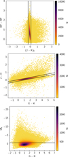 |
Fig. A.1 Distribution of the OB stars selected Gaia Collaboration (2023) in the colour-colour and colour-magnitude diagrams used for the selection of the targets of the SDSS-V mwm_ob program presented in Zari et al. (2021). The solid black lines represent the selection criteria in Zari et al. (2021). |
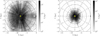 |
Fig. A.2 Distribution of the sample presented in D23 in the Galactic plane. The top panel shows the entire sample, the bottom panel shows only the sources with Gaia DR3 line-of-sight velocities. The yellow star represents the Sun’s position. The dashed black circles have radii R= 2, 4, 6, 8, 10 kpc. The solid lines indicate constant Galactic longitudes. |
Appendix B Maps of velocity dispersion
Figure B.1 (left) shows the maps of the velocity dispersion σR derived by using Eq. (4) in Section 3.1 for the HSS (top), and in Section 4.3 for the APOGEE DR17 RGB sample (bottom, see Section). The velocity dispersion of the hot star sample is usually between 10 and 20 km/s. This large value should not excessively surprise the reader, as the spatial scale of the map is large (the spaxel size is 250 × 250 pc). We note that the velocity dispersion of the HSS is remarkably smaller than the velocity dispersion of the APOGEE DR17 sample (see Fig. B.1 bottom left). This is expected, as the kinematic properties of the two samples are dramatically different, and older populations have larger velocity dispersion.
We estimated the velocity uncertainty on v̄R as  , where N* is the number of stars in a spaxel. Figure B.1 (right) shows the maps of the radial velocity uncertainty
  for the HSS (top) and the APOGEE DR17 RGB sample (bottom).
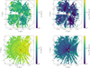 |
Fig. B.1 Velocity dispersion (left) and velocity uncertainty (right) maps for the Hot Star Sample (top) and for the APOGEE DR17 sample (bottom). The colorbars extend from 1 km/s to 60 km/s in all panels. The yellow star marks the location of the Sun, in X, Y=(−8.2, 0). The dashed circles have radii separated by ΔR = 2 kpc. |
Appendix C Simulation of a population of stars with 50% binary fraction
As explained in Section 2.3, we verified that the average is a good estimator of the centre of mass motion of our sample by simulating a population of stars with 50% binary fraction, observed at the same MJD’s and with the same vl.o.s. errors as our sample. Figure C.1 shows histogram distributions of the average velocities for simulated (blue) and single (orange) stars. For single stars, the dispersion around the average value roughly coincides with the measurement errors. For binary stars, the spread is larger. The main contribution to the spread is due to binary stars that have only a single-epoch observation. We repeated our analysis by including only stars observed at ≥ 2 epochs, and we did not find any significant difference on our main results (Figs. 7 and 11).
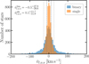 |
Fig. C.1 Distribution of average line-of-sight velocities for a simulated population of stars with 50% binary fraction, observed with the same cadence as our sample of Hot Stars, and with the same vl.o.s. errors. Vertical lines mark the 16th/84th percentile for single (dashed) and binary (dotted) stars. Annotated labels report the mean and corresponding uncertainty intervals derived from the 16th and 84th percentiles. |
Appendix D Selection of the APOGEE DR17 sample of disc stars
To compare the motions of young massive stars and old disc sources in Sec. 4 we made use of the astroNN value-added catalogue (Leung & Bovy 2019a) of abundances, distances, and ages for APOGEE DR17 sources5. astroNN is an open-source Python package developed for the neural network trained on the APOGEE data and is designed to be a general package for deep learning in astronomy. The APOGEE-astroNN catalogue contains results from applying astroNN neural nets on APOGEE DR17 spectra to infer stellar parameters, abundances trained with ASPCAP DR17 (Shetrone et al. 2015; García Pérez et al. 2016; Smith et al. 2021, Holtzman et al., in prep), distances retrained with Gaia eDR3 (Gaia Collaboration 2021) from Leung & Bovy (2019b), and ages trained with APOKASC-2 (Mackereth et al. 2019) in combination with low-metallicity asteroseismic ages (Montalbán et al. 2021). Following Hackshaw et al. (2024), we employed the following cuts to select disc stars:
We selected stars in the plane by requiring |b|<10 deg.
We used the astroNN distance and distance errors to select stars with distance errors <30%.
To select red giants, we restricted our sample to stars in the effective temperature range 3500< Teff <5000 K, and with log g<3.6 dex.
Finally, we select stars following disc kinematics by using the Toomre diagram (see Fig. D.1). In particular we selected stars with −600<V<200 km/s and
 . This is a broad selection, that nevertheless allows to remove outliers.
astroNN provides pre-computed positions, velocities, and actions. Positions and velocities were computed assuming the Sun is located at 8.125 kpc from the Galactic center (GRAVITY Collaboration 2019), 20.8 pc above the Galactic midplane (Bennett & Bovy 2019), and has radial, rotational, and vertical velocities of −11.1, 242, and 7.25 km/s. Actions were computed by integrating the stellar orbits with the Gala code (Price-Whelan 2017). The mass-model of the Milky Way used for the gala.dynamics.orbit function was the MilkyWayPotential2022, which has been fitted to the rotation curve in Eilers et al. (2020) and incorporates the phase-space spiral in the solar neighborhood set by E. Darragh-Ford et al. (2023).
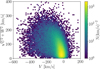 |
Fig. D.1 Toomre diagram for the APOGEE DR17 astroNN sample described in Sec. D. |
All Tables
All Figures
|
Fig. 1 Distribution in sky (Galactic coordinates) of sources of SDSS-V mwm_ob program observed until February 2025 (top, grey, 165 460 sources) and of the filtered sample described in Section 2.2 (bottom, orange, around 45 487 stars). The sources of the mwm_ob program are mostly located in the Galactic plane and the MCs. |
| In the text | |
|
Fig. 2 Flowchart illustrating steps to construct HSS described in Sect. 2.2. The notation v.theta-3* indicates that the numbers are provisional and refer to the specific Robostrategy version named theta-3 (Blanton et al. 2025). The survey efficiency has improved, and the final number of observed targets will likely increase in the future. |
| In the text | |
|
Fig. 3 Comparison between BOSS Net parameters and Gaia DR3 ESP-HS parameters for the hot-stars sample. The dashed orange lines correspond to the 1:1 relation. |
| In the text | |
|
Fig. 4 Kiel diagram of sources in mwm_ob program (grey histogram) passing the quality cuts described in Section 2.2 and of those in the HSS (coloured histogram). The dashed vertical lines mark the following temperatures: 31 000 K (O9.5V type star), 17 000 (B3V type star), 10 400 K (B9V type star), 7400 K (A9V type star), and 6050 K (F9V type star). |
| In the text | |
|
Fig. 5 Comparison between Gaia DR3 and SDSS-V XCSAO/Boss net line-of-sight velocities (in km/s). The orange dashed line corresponds to the 1:1 relation. |
| In the text | |
|
Fig. 6 Azimuthal velocity vφ as function of galactocentric radius, R. The histogram shows the azimuthal velocity distribution. The dashed orange lines indicate the boundaries of our selection: between 190 and 250 km/s. |
| In the text | |
|
Fig. 7 Distribution of hot-star sample in Galactic plane. The left panel shows the density distribution of the sources. The right panel shows the distribution of sources colour-coded by their galactocentric radial velocity (computed as described in the text). In both panels, the Sun is in X, Y=(−8.2, 0) kpc, and it is indicated by the yellow star. The Galactic centre is in X, Y = (0, 0) kpc. The dashed circles have radii of 2, 4, 6, 8, and 10 kpc. The solid lines indicate constant Galactic longitudes. |
| In the text | |
|
Fig. 8 Mean log-age map of hot-star sample in the Galactic plane. The mean ages are computed only for spaxels with more than five stars. The dashed circles have radii of 2, 4, and 6 kpc. The yellow star indicates the Sun’s position. The solid lines indicate constant Galactic longitudes. |
| In the text | |
|
Fig. 9 Comparison between ages for clusters determined in this work and by Hunt & Reffert (2023) and Cantat-Gaudin et al. (2020). The colour bar represents the number of hot stars in the cluster. The dashed line represents the 1: 1 relation in both panels. |
| In the text | |
|
Fig. 10 Comparison between density distribution of OB stars, the spiral-arm model from Reid et al. (2019), and the radial velocity asymmetries. In the left panel and central panels, the solid black contours represent the 0 and 0.5 density-contrast levels. In the right panel, the spiral arms are named following Reid et al. (2019): Outer Arm; Perseus Arm; Local Arm; Sagittarius-Carina Arm; Scutum-Centaurus Arm. In the three panels, the yellow star indicates the Sun’s position in X, Y=−8.2, 0 kpc, and the Galactic centre is located in X, Y = 0, 0 kpc. The dashed lines represent circle radii of 2, 4, and 6 kpc. The solid lines indicate constant Galactic longitudes. |
| In the text | |
|
Fig. 11 Density distribution of young (<30 Myr; left) and older (>150 Myr) sources. In the left panel, star forming regions are indicated. The solid contour lines represent the density distribution of all sources (Fig. 10, left) and are computed as described in Sect. 4. The labels highlight some of the more prominent OB associations (their locations are from Table 1 of Wright 2020). The solid lines indicate constant Galactic longitudes. |
| In the text | |
|
Fig. 12 Density distribution (left) and galactocentric radial velocities (right) of the gaiauriga mock stellar catalogue for young (top) and old (bottom) sources. The black lines outline the contours of the density distribution. The black dot indicates the Galactic centre, the yellow star the Sun’s position. The dashed black lines mark concentric circles at ΔR = 2 kpc. The v̄R> feature for R ≲ 5 kpc in the right panels is due to the effect of the bar on the kinematics of sources in the inner galaxy. The solid lines indicate constant Galactic longitudes. |
| In the text | |
|
Fig. 13 Distribution of red giant stars in Milky Way disc from APOGEE DR17. The red giant stars are colour-coded by their average galactocentric radial velocity. The location of the Sun is indicated by the yellow star. The dashed black lines mark concentric circles at ΔR = 2 kpc. The solid lines indicate constant Galactic longitudes. The region within 5 kpc of the Galactic centre is masked as the stellar motions in that region are influenced by the bar. |
| In the text | |
|
Fig. A.1 Distribution of the OB stars selected Gaia Collaboration (2023) in the colour-colour and colour-magnitude diagrams used for the selection of the targets of the SDSS-V mwm_ob program presented in Zari et al. (2021). The solid black lines represent the selection criteria in Zari et al. (2021). |
| In the text | |
|
Fig. A.2 Distribution of the sample presented in D23 in the Galactic plane. The top panel shows the entire sample, the bottom panel shows only the sources with Gaia DR3 line-of-sight velocities. The yellow star represents the Sun’s position. The dashed black circles have radii R= 2, 4, 6, 8, 10 kpc. The solid lines indicate constant Galactic longitudes. |
| In the text | |
|
Fig. B.1 Velocity dispersion (left) and velocity uncertainty (right) maps for the Hot Star Sample (top) and for the APOGEE DR17 sample (bottom). The colorbars extend from 1 km/s to 60 km/s in all panels. The yellow star marks the location of the Sun, in X, Y=(−8.2, 0). The dashed circles have radii separated by ΔR = 2 kpc. |
| In the text | |
|
Fig. C.1 Distribution of average line-of-sight velocities for a simulated population of stars with 50% binary fraction, observed with the same cadence as our sample of Hot Stars, and with the same vl.o.s. errors. Vertical lines mark the 16th/84th percentile for single (dashed) and binary (dotted) stars. Annotated labels report the mean and corresponding uncertainty intervals derived from the 16th and 84th percentiles. |
| In the text | |
|
Fig. D.1 Toomre diagram for the APOGEE DR17 astroNN sample described in Sec. D. |
| In the text | |
Current usage metrics show cumulative count of Article Views (full-text article views including HTML views, PDF and ePub downloads, according to the available data) and Abstracts Views on Vision4Press platform.
Data correspond to usage on the plateform after 2015. The current usage metrics is available 48-96 hours after online publication and is updated daily on week days.
Initial download of the metrics may take a while.