| Issue |
A&A
Volume 703, November 2025
|
|
|---|---|---|
| Article Number | A273 | |
| Number of page(s) | 8 | |
| Section | Extragalactic astronomy | |
| DOI | https://doi.org/10.1051/0004-6361/202556708 | |
| Published online | 19 November 2025 | |
The X-ray–UV luminosity relation of eROSITA quasars
1
Center for Astrophysics | Harvard & Smithsonian, 60 Garden Street, Cambridge, MA 02138, USA
2
INAF – Istituto di Astrofisica Spaziale e Fisica Cosmica Milano, Via A.Corti 12, 20133 Milano, Italy
3
Dipartimento di Fisica e Astronomia, Universita‘ di Firenze, Via G. Sansone 1, I-50019 Sesto Fiorentino, Firenze, Italy
4
INAF “Osservatorio Astrofisico di Arcetri, Largo Enrico Fermi 5, I-50125 Firenze, Italy
5
European Space Agency (ESA), European Space Research and Technology Centre (ESTEC), Keplerlaan 1, 2201 AZ Noordwijk, The Netherlands
6
Scuola Normale Superiore, Piazza dei Cavalieri 7, I-56126 Pisa, Italy
⋆ Corresponding author: This email address is being protected from spambots. You need JavaScript enabled to view it.
Received:
1
August
2025
Accepted:
15
October
2025
Abstract
The nonlinear relation between the UV and X-ray luminosity in quasars has been studied for decades. However, as no comprehensive model can yet explain it, its investigation still relies on observational efforts. This work focuses on optically selected quasars detected by eROSITA. We present the properties of the sources collected in the eROSITA early data release (eFEDS) and those resulting from the first six months of the eROSITA all-sky survey (eRASS1). We focus on the subset of quasars bright enough in the optical/UV band to avoid an “Eddington bias” toward X-ray brighter-than-average spectral energy distributions. The final samples include 1248 and 519 sources for eFEDS and eRASS1, up to redshift z ≈ 3 and z ≈ 1.5, respectively. We find that the X-ray–UV luminosity relation does not evolve significantly with redshift, and its slope is in perfect agreement with previous compilations of quasar samples. The intrinsic dispersion of the relation is about 0.2 dex, which is small enough for possible cosmological applications. However, due to the limited redshift range and statistics of the current samples, we cannot obtain significant cosmological constraints yet. We show how this is going to change with the future releases of eROSITA data.
Key words: accretion / accretion disks / galaxies: active / quasars: general / X-rays: galaxies
© The Authors 2025
 Open Access article, published by EDP Sciences, under the terms of the Creative Commons Attribution License (https://creativecommons.org/licenses/by/4.0), which permits unrestricted use, distribution, and reproduction in any medium, provided the original work is properly cited.
This article is published in open access under the Subscribe to Open model. This email address is being protected from spambots. You need JavaScript enabled to view it. to support open access publication.
1. Introduction
Quasi-stellar objects (QSOs) are extremely powerful and stable astrophysical sources. They are known up to z ≈ 10 (Bogdán et al. 2024) and as such, in principle, represent perfect standard candles.
In a series of works starting from 2015 (Risaliti & Lusso 2015; Lusso & Risaliti 2016, 2017; Risaliti & Lusso 2019; Lusso et al. 2020; Bisogni et al. 2021), our group has proven that as candles QSOs are “standardizable” through the well-known, nonlinear relation between their UV and X-ray luminosity (Tananbaum et al. 1979; Lusso et al. 2010). This relation can be expressed as  with γ ≈ 0.6, and it links the optical/UV emission of the disk to the X-ray emission of the corona. Coupled with a properly selected sample of QSOs, this allows us to expand the Hubble diagram beyond the z ≈ 2 limit of currently detected type Ia supernovae (Risaliti & Lusso 2019).
The method developed by our group is based on the assumption that the observed dispersion of the X-ray–UV luminosity relation is entirely due to observational issues (e.g., dust and gas absorption, variability, and the orientation of the source) and, therefore, that there exists a physical mechanism that entwines the UV and X-ray emissions of active galactic nuclei (AGNs). In our previous work we have shown that this assumption is well motivated, by reducing the dispersion of the relation from the historical value of 0.8 dex (Tananbaum et al. 1979) to 0.20 − 0.22 dex by selecting only blue unobscured QSOs (Lusso & Risaliti 2016; Lusso et al. 2020), and finally reaching 0.09 dex by considering a sample with high-quality, targeted X-ray observations, and performing a full spectral analysis for each source (Sacchi et al. 2022). Our group has also demonstrated that the residual dispersion can be explained almost entirely by considering inclination effects and the intrinsic variability of the considered sources (Signorini et al. 2024).
To date, however, the study of this relation has relied entirely on observational efforts. Despite several attempts, a complete physical model capable of explaining the observed relation between the X-ray and UV luminosities, and describing the mechanism through which the accretion disk and the hot corona exchange energy, is still missing. Models invoking, for example, the reconnection of magnetic loops above the disk as a source of the primary X-ray radiation (Lusso & Risaliti 2017), or modified viscosity prescriptions coupled with outflowing Comptonizing coronae and/or highly spinning black holes (Arcodia et al. 2019), seemed promising. However, they fail to simultaneously reproduce the slope, normalization, and small dispersion of the observed relation.
The latest compilations of our QSO samples (Lusso et al. 2020; Bisogni et al. 2021) were based on the most recent releases (at that time) of the Sloan Digital Sky Survey (SDSS DR14; Pâris et al. 2018), the Chandra X-ray Catalog (CXC2.0; Evans et al. 2010), and the Fourth XMM-Newton Serendipitous Source Catalog (4XMM-DR9; Webb et al. 2020), and included ≈2500 sources. These samples were successfully employed to build a Hubble diagram that highlighted a ≃4σ tension with the standard flat Λ cold dark matter model (H0 = 70 km/s/Mpc, ΩM = 0.3, and ΩΛ = 1 − ΩM; e.g., Risaliti & Lusso 2019; Lusso et al. 2020; Bargiacchi et al. 2021).
This tension was interpreted by some authors (Khadka & Ratra 2020, 2021, 2022; Montiel et al. 2025) as proof of the inapplicability of QSOs at large for cosmological studies, attributing it to either a biased selection or an evolution of the parameters of the relation with redshift. This and other forms of criticism have been addressed in depth in a dedicated publication by Lusso et al. (2025), who show that QSOs are reliable standardizable candles unless the parameters of the X-ray–UV luminosity relation experience a sudden change at z > 1.5, i.e., where the extremely good agreement between QSO- and supernova-derived distances can no longer be observationally demonstrated due to the dearth of probes of the latter. In other words, such a glitch would imply that QSOs below and above z = 1.5 accrete in different ways, which is thought to be highly unlikely.
Irrespective of the cosmological implications, the lack of a comprehensive accretion theory behind the X-ray–UV relation demands a constant observational scrutiny of the relation itself. To this aim, we explored the X-ray and UV properties of a sample of QSOs detected by the extended ROentgen Survey with an Imaging Telescope Array (eROSITA; Predehl et al. 2021). This effort is key, as it demonstrates both the independence of the relation from the instrument, dataset, and X-ray observational strategy (whether in pointed, serendipitous, or survey mode) and the transformative potential of forthcoming eROSITA data releases. eROSITA is the primary instrument of the Russian-German Spektrum-Roentgen-Gamma (SGR) mission, which was successfully launched in July 2019 (Sunyaev et al. 2021). With an on-axis sensitivity at 1 keV comparable with that of XMM-Newton but coupled with a wider field of view and better spectral resolution (Predehl et al. 2021), eROSITA represents the ideal instrument to build a vast sample of QSOs for the study of accretion physics and its possible cosmological applications. To date, the eROSITA collaboration has published two datasets: (i) the eROSITA Final Equatorial Depth Survey (eFEDS; Brunner et al. 2022), covering an area of 140 deg2 with an average exposure time of 2 ks, and (ii) the first six months of the SGR/eROSITA all-sky survey (eRASS1; Merloni et al. 2024), whose proprietary rights lie with the German eROSITA consortium, covering half of the sky (≈20 000 deg2) with an average exposure time of 250 s.
This paper is structured as follows. In Sect. 2 we report the analysis of the sources included in the eFEDS data release. In Sect. 3 we present the results based on eRASS1 sources, and in Sect. 4 we draw our conclusions and show the predictions for the future releases of eROSITA data. Everywhere in this manuscript, the luminosity values, when reported, are computed by assuming a standard flat Λ cold dark matter cosmology with ΩM = 0.3 and H0 = 70 km s−1 Mpc−1, unless stated otherwise.
2. eFEDS sources
2.1. Sample selection
Released in 2021, eFEDS (Brunner et al. 2022) covers a sky area of 140 deg2 with an average exposure time of 2 ks, mimicking the expected final depth that the eROSITA all-sky survey will achieve. The full eFEDS catalog includes ≈28 000 sources; for our purposes, we employed the eFEDS AGN Catalog (Liu et al. 2022), which comprises 21 952 unique sources spanning from z ≈ 0.004 up to z = 8 (shown in red in Fig. 1).
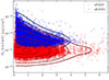 |
Fig. 1. Flux in the 0.5–2 keV band versus redshift for the source in the eFEDS (red circles) and eRASS1 (blue squares) parent samples. Given the high density of objects, contours with matching colors have been added to highlight the sources’ distributions. |
As broadly discussed in previous works (Risaliti & Lusso 2019; Lusso et al. 2020; Bisogni et al. 2021; Signorini et al. 2023), we adopted the 2500 Å and 2 keV monochromatic flux densities as proxies of the accretion disk and corona emission, respectively. For the eFEDS sample, a complete X-ray spectral analysis is available, as is multiwavelength coverage (Salvato et al. 2022). In particular, all sources possess Hyper Suprime-Cam (HSC; Aihara et al. 2018) and/or Kilo-Degree Survey (KiDS; Kuijken et al. 2019) optical photometry. Hence, we adopted the 2500 Å and 2 keV monochromatic flux densities values provided by the catalog.
The X-ray–UV relation for the sample at this stage is affected by a large scatter due to the presence of sources whose X-ray and/or UV flux is absorbed or enhanced by several different effects (see Fig. 3). Therefore, to study the intrinsic relation between the disk and the corona, we rid the sample of these contaminants. To this end, we followed the approach developed in our previous works (Risaliti & Lusso 2015, 2019) and detailed in Lusso et al. (2020) and Bisogni et al. (2021): we removed sources that were (i) affected by dust-absorption or host-galaxy contamination in the UV band, (ii) obscured in the X-ray band, or (iii) radio-loud (RL).
The radio emission from RL QSOs can affect the estimate of the 2-keV monochromatic flux, increasing it with respect to radio-quiet AGNs (Zamorani et al. 1981; Wilkes & Elvis 1987). Symmetrically, objects exhibiting broad absorption lines (BALs) in the UV are thought to be more X-ray-obscured with respect to non-BAL AGNs (Green et al. 1995; Gallagher et al. 1999; Brandt et al. 2000; but see also Hiremath et al. 2025). In any case, the presence of BALs complicates the determination of the continuum, making the intrinsic UV emission prone to being miscalculated. To exclude the sources affected by these factors, we crossmatched the eFEDS sample with the Faint Images of the Radio Sky at Twenty-cm (FIRST) and the National Radio Astronomy Observatory (NRAO) VLA Sky Survey (NVSS) catalog and the Sloan Digital Sky Survey (SDSS) DR16Q catalog (Lyke et al. 2020), and eliminated all the sources with a radio-loudness parameter (R = F6 cm/ F2500 Å) > 10 and/or a balnicity index (BI_CIV) > 0.
As the presence of dust along the line of sight and/or the contamination by host-galaxy light could affect the measurement of the 2500 Å monochromatic flux, we removed from the sample all the reddened sources. To this end, we computed the slope of the rest-frame photometric spectral energy distribution (SED) between 1450 and 3000 Å (Γ2). The photometric SEDs were obtained employing HSC magnitudes or, if these were not available, KiDS magnitudes. This procedure is usually also adopted to derive the rest-frame 2500 Å monochromatic flux densities, but in this case this quantity is taken directly from the catalog. We eliminated from our sample all the sources with |Γ2 − 0.4|> 1.1. This choice slightly differs from the one adopted in previous works, where, along with Γ2, the slope of the SED computed between 0.3 and 1 μm (Γ1) was also employed to eliminate all sources outside a circle in the Γ1 − Γ2 plane of radius 1.1 centered on (0.85, 0.40). This choice corresponds to a reddening E(B − V)≲0.1. The first reason for the relaxation of this requirement is that the UV/optical color selection affects the cleaning procedure less than the criteria applied to the X-ray band (such as Eddington bias and photoelectric absorption). Secondly, in doing so, we do not need infrared data in order to correctly estimate Γ1, which largely falls in the near-/mid-infrared regime starting from a relatively low redshift. Thirdly, the criterion we adopted, which considers only Γ2, still corresponds to a reddening E(B − V)≲0.1 given that, for the SED of QSOs, reddening affects slope Γ2 more prominently than slope Γ1 (see Trefoloni et al. 2024 for an in-depth discussion of the effects of optical/UV spectral selections and properties). To reduce possible contamination by the host galaxy, we also removed all objects with a redshift (z) of ≤0.48 (Bisogni et al. 2021).
In all of the works presented by our group, the quality of the X-ray observations is what most strongly affects the dispersion observed in the X-ray–UV luminosity relation (see Sacchi et al. 2022; Signorini et al. 2024 for a full discussion); therefore, the X-ray cleaning process is to be addressed with particular care. The main issue affecting the X-ray emission of QSOs is photoelectric absorption. To exclude absorbed objects, the criterion applied by our group relies on estimating the photometric slope of the X-ray spectrum (ΓX) and excluding all sources that significantly deviate from the typical slope of unabsorbed QSOs (ΓX = 1.9; e.g., Risaliti et al. 2009). As photoelectric absorption is naturally heavier in the soft band, flattening the X-ray spectrum and resulting in smaller values of ΓX, we usually excluded sources with ΓX − ΔΓX ≤ 1.7 (where ΔΓX is the error on the photon index). On the other hand, an excessively steep spectrum could be due to observational issues, so we also excluded sources with ΓX > 2.8. For the eFEDS sample, however, contrary to the eRASS1 sample described below (see Sect. 3), full spectroscopic analysis is available; hence, we directly adopted the classification provided by Liu et al. (2022) and removed from our sample all the sources flagged as “uninformative” or “absorbed,” retaining only sources flagged as “unabsorbed” (NHclass = 2). In addition to this, we excluded all objects with a low signal-to-noise ratio in the soft band (S/N < 1). This ensures that the X-ray spectroscopic analysis is reliable. This choice allowed us to efficiently remove absorbed sources by exploiting the full potential of the complete X-ray spectroscopy available for eFEDS sources.
Number of sources passing each filter.
The final factor we had to account for is the Eddington bias. QSOs exhibit intrinsic variability, and a source with an intrinsic flux close to the detection limit of the considered instrument would only be detected during a positive flux fluctuation. This flattens the slope of the X-ray–UV luminosity relation, as sources with low UV flux are more easily detected in a high X-ray flux state. To correct for this bias, we employed the same strategy adopted in our previous works and described at length in Lusso & Risaliti (2016). Briefly, we assumed a slope γ = 0.6 for the X-ray–UV luminosity relation and adopted it to compute the expected monochromatic flux density (fexp) at 2 keV, starting from that measured at 2500 Å. Then we compared this expected flux density with the sensitivity limit (flim) of the observation in which the object was detected. The sensitivity limit was computed based on the exposure time at the location of the source, provided by the catalog, and the sensitivity curves described in Merloni et al. (2012). In practice, one should remove all the sources for which log fexp ≤ log flim + kδ, where δ is the observed dispersion of the sample at hand, and k is a multiplicative factor. Determining the value of k is clearly key in correcting for the Eddington bias, and the method through which this quantity is derived has been described at length in Lusso & Risaliti (2016) and Risaliti & Lusso (2019). As mentioned, the Eddington bias tends to flatten the slope of the relation; hence, if k is underestimated, one expects a lower value of γ. On the contrary, if k is overestimated, unbiased sources are removed, reducing the sample size and increasing the intrinsic dispersion (δ). The optimal value of k was then determined by monitoring the values of γ and δ for different values of k. Once γ remains stable and only δ increases with k, the optimal value of k has been reached.
For the eFEDS sample, we determined this optimal value to be k = 0. This choice is equivalent to selecting sources with fexp ≥ flim, so, in principle, a residual bias is still present. In fact, a source experiencing a negative fluctuation is rejected and one undergoing a positive fluctuation is retained. However, for k = 0 the slope of the relation is already stable and compatible with the previous values obtained in the literature. This means that by increasing k we obtain values of γ that are consistent with that obtained using k = 0, but with reduced statistics (and therefore larger uncertainties). The best value being k = 0 differs from previous studies and can be explained given the specifics of the eROSITA sample. Contrary to samples collected by other X-ray observatories, here the flux limits have been derived using sensitivity curves published before the deployment of eROSITA, which might be slightly overestimated. Furthermore, the observational strategy of eROSITA, consisting of repeated scans of the sky, actively mitigates the variability of each individual source, making this bias less critical for the ultimate determination of the slope of the relation γ.
The final sample (after removing four additional outliers; see below) is composed of 1248 QSOs, shown in red in Fig. 2. A breakdown of how many sources were removed by each filter is presented in Table 1.
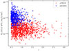 |
Fig. 2. Flux in the 0.5–2 keV band versus redshift for sources in the eFEDS (red circles) and eRASS1 (blue squares) final samples. |
2.2. X-ray–UV relation
Figure 3 shows the X-ray luminosity as a function of the UV luminosity (computed from the 2 keV and the 2500 Å monochromatic flux densities, respectively) for the QSOs in the eFEDS final sample (red data points). In the same figure we report the sources composing the two parent samples we adopted (in gray), and one can straight away appreciate how the filtering process we adopted reduced the dispersion of the samples significantly. Furthermore, we note that the final sample is shifted toward lower values of LX. This is a further manifestation of the Eddington bias affecting the parent samples, which likely also involves the sources filtered out through the selection criteria applied to the X-ray photon index.
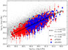 |
Fig. 3. X-ray–UV relation. The eFEDS and eRASS1 data are shown with red circles and blue squares, respectively. The best fits for the samples are reported by the dashed and dash-dotted lines. The gray dots represent the eRASS and eFEDS parent sample, before any filtering has been applied. |
To quantify this, we fitted the relation with the Python package emcee (Foreman-Mackey et al. 2013), a pure-Python implementation of Goodman and Weare’s affine invariant Markov chain Monte Carlo ensemble sampler. We imposed a 3σ clipping criterion, which eliminated four outliers. We obtained a best-fit value for the slope of the relation of γ = 0.62 ± 0.01. This value is in excellent agreement with those found in our group’s previous works for different samples.
Previous studies have shown that uncertainties in X-ray and UV luminosities alone cannot account for the observed scatter around the best-fit line. To model this, we introduced the parameter δ, which represents the intrinsic dispersion of the relation. This dispersion arises from QSO variability, inclination effects, and the “intrinsic” spread of the relation itself. However, without a complete physical model, we cannot precisely quantify the contribution of this intrinsic spread. Nonetheless, analyses of the Lusso et al. (2020) sample and high-quality, smaller subsamples suggest that variability and inclination can explain a significant part of the observed dispersion, leaving little room for additional scatter from the underlying physical processes (Sacchi et al. 2022; Signorini et al. 2024). For our sample, the best-fit value of the intrinsic dispersion is δ = 0.22 dex (for the combined parent sample, the dispersion is δ = 0.36 dex). This value is compatible with previous compilations of QSO samples, suggesting that the eFEDS sample is affected by the same residual biases.
We cannot directly probe any evolution of the relation parameters with redshift; however, we can indirectly investigate possible systematic trends by splitting our sample into narrow redshift bins and employing the fluxes as proxies of the luminosities. This approach has already been exploited to prove the non-evolution of the relation up to redshift ≈3.5 for the XMM-Newton and Chandra QSO samples (Risaliti & Lusso 2019; Lusso et al. 2020; Bisogni et al. 2021). We divided the sample into eight redshift bins, from z = 0.48 up to z = 3. The width of the bins was varied to ensure that there are enough statistics in each bin and that the dispersion in distances within each bin is smaller than that in the luminosity relation [see][for a full discussion on this]lusso25. This guarantees that using fluxes as proxies of luminosities is a sound approximation.
Figure 4 shows the best-fit parameters γ and δ (slope and intrinsic dispersion) of the flux–flux relation (the fits of the objects in the individual bins are reported in Appendix B), along with their uncertainties. The data show no evident trend with redshift for either the slope of the relation or the dispersion. The average slope is ⟨γ⟩ = 0.55 ± 0.04, and the average intrinsic dispersion is ⟨δ⟩ = 0.22 ± 0.02. This result confirms those obtained in previous works based on data taken with different telescopes: the slope of the relation does not evolve with redshift, and this strongly suggests that the accretion mechanism responsible for the QSO phenomenon is universal. In turn, this enables the standardization of QSOs for cosmological usage.
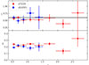 |
Fig. 4. Parameters of the flux–flux relation as a function of redshift. Top: slope (γ). The gray line indicates the standard 0.6 value for the slope. Bottom: intrinsic dispersion (δ). The eFEDS and eRASS1 data are shown in blue and red, respectively. |
3. eRASS1 sources
3.1. Sample selection
The German eROSITA consortium released the first six months of data of the SGR/eROSITA all-sky survey (eRASS1) in early 2024. Covering half of the sky, corresponding to ≈20 000 deg2 with an average exposure time of 250 s, this rich dataset includes ≈930 000 individual sources (Merloni et al. 2024). We built the parent sample of cosmological QSOs by crossmatching this catalog with the SDSS DR16Q catalog (Lyke et al. 2020), with a matching radius of 15 arcsec (corresponding to roughly half of the eROSITA point spread function in scanning mode). This produced 24 375 unique matches.
We cleaned this sample in the same fashion adopted for the eFEDS one. We removed BAL objects by exploiting the balnicity index, and we removed RL sources if they were detected in the radio in the FIRST/NVSS catalog. To exclude sources that might be affected by host-galaxy contamination, all sources with redshifts of < 0.48 were also removed.
Unlike for eFEDS objects, for the sources in eRASS1, full X-ray spectroscopic information is not available. Hence, to remove sources affected by photoelectric absorption, we adopted the method described at length in Risaliti & Lusso (2019) and Lusso et al. (2020). Briefly, we exploited the fluxes reported in the X-ray catalog in the soft (0.5–1 keV) and medium (1–2 keV) bands to derive both the monochromatic 2-keV flux density (corrected for Galactic absorption) and the X-ray photon index (ΓX), with relative errors. To do so, the broadband fluxes were transformed into monochromatic flux densities at the respective “pivot” points. This ensures that the results do not depend upon the choice of photon index adopted to convert the detected count rate into energy flux, and it minimizes the uncertainties on the photon index and flux. The efficiency and robustness of this procedure have been tested at length by our group, and we will not address it further here. We also excluded all sources with ΓX < 1.7 or ΓX > 2.8.
Dust obscuration and the Eddington bias were addressed in the same fashion as described for the eFEDS sample. For the Eddington bias, the same choice of k = 0 was adopted.
Table 1 presents a breakdown of the sources excluded by each filter. The final eRASS1 sample (after removing four additional outliers; see below) includes 519 individual sources. This is a factor of ≳2 fewer than the eFEDS sample. Given that the parent samples have similar sizes, we investigated which filters affected the size of the final samples most heavily: all filters removed about the same fraction of sources except for the Eddington bias, which removed ≈75% of the eFEDS sources and ≈90% of the eRASS1 sample. In other words, one-fourth of the eFEDS sources survived the Eddington bias filter, while only one-tenth of the eRASS1 sources did. This is due to the difference in depth of the two surveys, the former being eight times deeper than the latter.
3.2. X-ray–UV relation
We proceeded to fit the X-ray–UV relation for the 519 objects composing the final eRASS1 sample in the same fashion adopted for the eFEDS sample. In this case, too, we imposed a 3σ clipping cut that removed four outliers. The best-fit slope of the relation is γ = 0.63 ± 0.02, and the intrinsic dispersion is δ = 0.20. These values are both in perfect agreement with previous studies and with the eFEDS sample. Figure 3 shows the objects in the eRASS1 sample and the best-fit relation.
For this sample, too, we explored possible redshift dependences of the relation parameters, binning the sources in narrow redshift bins and adopting the fluxes as proxies of the luminosities. The redshift range spanned by the sources in the eRASS1 sample is relatively narrow; hence, we could explore the properties of the relation only up to redshift 1.5. Nonetheless, in the accessible range, we observed no slope evolution, and we obtained ⟨γ⟩ = 0.58 ± 0.04 and ⟨δ⟩ = 0.20 ± 0.01, in agreement with the literature results and the average values for these parameters obtained for the eFEDS sample.
Regardless of the limited size of the presented sample (as well as of the eFEDS one), these relatively small values of intrinsic dispersion (δ ≃ 0.2 dex) stem from the quality of eROSITA datasets. We attribute this to the way eROSITA collects data, performing repeated scans of the sky and de facto averaging the flux of each source. Furthermore, eROSITA has been designed for surveys, and hence the vignetting and its associated uncertainties are significantly less than those affecting serendipitous Chandra or XMM-Newton observations. Indeed, the values of intrinsic dispersion we obtained are comparable with previous compilations of samples of cosmological QSOs that took into account and averaged the flux of the sources over multiple observations (Lusso et al. 2020). This fact, coupled with the little overlap of these datasets with those obtained with other facilities (e.g., XMM-Newton; see Appendix A for a more in-depth comparison), highlights the statistical potential of present and future eROSITA data.
4. Future eROSITA data releases
The analysis performed on the eFEDS and eRASS1 datasets highlights how the former outperforms the latter in terms of final sample size, depth, and redshift range. This might seem surprising, as eRASS1, although eight times shallower, covers a more than two orders of magnitude wider sky area. However, one has to consider that the luminosity function of QSOs is extremely steep, and hence small increments in depth correspond to a large increase in the number of detected sources. Most importantly, however, all of the sources in eFEDS had dedicated optical follow-up, while for eRASS1 we had to rely on the crossmatch with SDSS DR16Q. How much this affects our analysis can be seen by comparing the sizes of the parent samples, which, as already noted in Sect. 3, were about the same.
While this dramatically affects the current status of publicly available eROSITA data, future releases will offer much richer opportunities. In particular, the next release of eROSITA data will coincide with the publication of the SDSS-V (mid 2026), which is currently performing optical follow-ups of eROSITA-detected sources.
We can roughly estimate the improvement in the final sample size by assuming that the optical coverage will be similar, for QSOs, to the one available for eFEDS sources. As eROSITA stopped operating after completing four and a half sky scans (eRASS:4.5), we can assume an average exposure roughly equal to half of the eFEDS exposure. We could hence straightforwardly take the eFEDS clean sample and apply an Eddington-bias filter as if the exposure time were half of the actual one. This left 591 sources, and we could simply multiply this number by the ratio between the sky area covered by eFEDS and that covered by the full eRASS:4.5 survey, which corresponds to half of the sky. We predict that the size of a QSO sample filtered following the procedure described above will amount to ≈78 000 sources. This is a giant leap in sample size with respect to the current state-of-the-art sample employed for cosmological studies (≈2000 sources; Lusso et al. 2020), which will allow us to study the X-ray–UV relation for QSOs in unprecedented detail.
This future sample will also offer precious opportunities to compare the QSO Hubble diagram with that built with type Ia supernovae. To grasp the potentiality of this giant improvement in sample size, we simulated the expected 78 000 sources of the eRASS:4.5 release, following the same redshift and UV flux distributions of the 591 sources in the eFEDS sample with a halved exposure time. We then generated, for each simulated source, its X-ray flux assuming the cosmographic model described by Bargiacchi et al. (2021) and an X-ray–UV relation characterized by a slope γ = 0.6 and a dispersion δ = 0.2 dex. The resulting Hubble diagram is presented in Fig. 5. The individual sources are not reported due to their large number; instead, they are represented by a density plot.
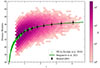 |
Fig. 5. Hubble diagram for the simulated eRASS:4.5 sample. The density plot represents individual sources. Averaged values are indicated by black data points. The type Ia supernovae from Scolnic et al. (2018) are in light green. The solid darker green line shows the cosmographic model. |
5. Conclusions
In this work we studied the X-ray–UV luminosity relation of unobscured, optically selected QSOs, detected by eROSITA. We compiled two samples, one based on the early data release of eROSITA observations (eFEDS) and the other the first data release of the mission (eRASS1). Notably, eROSITA data are from an all-sky survey, while previous compilations relied mainly on serendipitous observations. Exploiting these samples, we confirmed the results obtained when employing different independent observatories: the nonlinear relation between X-ray and UV luminosities for unobscured, blue QSOs is tight: its dispersion is entirely due to statistical and observational limits, and its parameters do not evolve with redshift. In this way, we confirm once more that the physics of accretion is independent from redshift evolution and, as a by-product, the exploitability of QSOs for cosmological studies, given their nature as “standardizable” candles. Finally, although the currently available datasets have little applicability to cosmological investigations, given the relatively limited redshift range they span, we demonstrated how the future releases of eROSITA data will represent a game changer in this domain, allowing us to build a Hubble diagram with almost 80 000 QSOs.
Acknowledgments
We thank the anonymous referee for insightful comments that improved the quality of this work. MS acknowledges support through the European Space Agency (ESA) Research Fellowship Programme in Space Science.
References
- Aihara, H., Arimoto, N., Armstrong, R., et al. 2018, PASJ, 70, S4 [NASA ADS] [Google Scholar]
- Arcodia, R., Merloni, A., Nandra, K., & Ponti, G. 2019, A&A, 628, A135 [NASA ADS] [CrossRef] [EDP Sciences] [Google Scholar]
- Bargiacchi, G., Risaliti, G., Benetti, M., et al. 2021, A&A, 649, A65 [NASA ADS] [CrossRef] [EDP Sciences] [Google Scholar]
- Bisogni, S., Lusso, E., Civano, F., et al. 2021, A&A, 655, A109 [NASA ADS] [CrossRef] [EDP Sciences] [Google Scholar]
- Bogdán, Á., Goulding, A. D., Natarajan, P., et al. 2024, Nat. Astron., 8, 126 [Google Scholar]
- Brandt, W. N., Laor, A., & Wills, B. J. 2000, ApJ, 528, 637 [CrossRef] [Google Scholar]
- Brunner, H., Liu, T., Lamer, G., et al. 2022, A&A, 661, A1 [NASA ADS] [CrossRef] [EDP Sciences] [Google Scholar]
- Evans, I. N., Primini, F. A., Glotfelty, K. J., et al. 2010, ApJS, 189, 37 [NASA ADS] [CrossRef] [Google Scholar]
- Foreman-Mackey, D., Hogg, D. W., Lang, D., & Goodman, J. 2013, PASP, 125, 306 [Google Scholar]
- Gallagher, S. C., Brandt, W. N., Sambruna, R. M., Mathur, S., & Yamasaki, N. 1999, ApJ, 519, 549 [Google Scholar]
- Green, P. J., Schartel, N., Anderson, S. F., et al. 1995, ApJ, 450, 51 [Google Scholar]
- Hiremath, P., Rankine, A. L., Aird, J., et al. 2025, MNRAS, 542, 2105 [Google Scholar]
- Khadka, N., & Ratra, B. 2020, MNRAS, 497, 263 [Google Scholar]
- Khadka, N., & Ratra, B. 2021, MNRAS, 502, 6140 [NASA ADS] [CrossRef] [Google Scholar]
- Khadka, N., & Ratra, B. 2022, MNRAS, 510, 2753 [NASA ADS] [CrossRef] [Google Scholar]
- Kuijken, K., Heymans, C., Dvornik, A., et al. 2019, A&A, 625, A2 [NASA ADS] [CrossRef] [EDP Sciences] [Google Scholar]
- Liu, T., Buchner, J., Nandra, K., et al. 2022, A&A, 661, A5 [NASA ADS] [CrossRef] [EDP Sciences] [Google Scholar]
- Lusso, E., Comastri, A., Vignali, C., et al. 2010, A&A, 512, A34 [NASA ADS] [CrossRef] [EDP Sciences] [Google Scholar]
- Lusso, E., & Risaliti, G. 2016, ApJ, 819, 154 [Google Scholar]
- Lusso, E., & Risaliti, G. 2017, A&A, 602, A79 [NASA ADS] [CrossRef] [EDP Sciences] [Google Scholar]
- Lusso, E., Risaliti, G., & Nardini, E. 2025, A&A, 697, A108 [NASA ADS] [CrossRef] [EDP Sciences] [Google Scholar]
- Lusso, E., Risaliti, G., Nardini, E., et al. 2020, A&A, 642, A150 [NASA ADS] [CrossRef] [EDP Sciences] [Google Scholar]
- Lyke, B. W., Higley, A. N., McLane, J. N., et al. 2020, ApJS, 250, 8 [NASA ADS] [CrossRef] [Google Scholar]
- Merloni, A., Lamer, G., Liu, T., et al. 2024, A&A, 682, A34 [NASA ADS] [CrossRef] [EDP Sciences] [Google Scholar]
- Merloni, A., Predehl, P., Becker, W., et al. 2012, ArXiv e-prints [arXiv:1209.3114] [Google Scholar]
- Montiel, A., Samario-Nava, S., Hidalgo, J. C., & Cabrera, J. I. 2025, ArXiv e-prints [arXiv:2509.08983] [Google Scholar]
- Pâris, I., Petitjean, P., Aubourg, É., et al. 2018, A&A, 613, A51 [Google Scholar]
- Predehl, P., Andritschke, R., Arefiev, V., et al. 2021, A&A, 647, A1 [EDP Sciences] [Google Scholar]
- Risaliti, G., & Lusso, E. 2015, ApJ, 815, 33 [NASA ADS] [CrossRef] [Google Scholar]
- Risaliti, G., & Lusso, E. 2019, Nat. Astron., 3, 272 [Google Scholar]
- Risaliti, G., Young, M., & Elvis, M. 2009, ApJ, 700, L6 [NASA ADS] [CrossRef] [Google Scholar]
- Sacchi, A., Risaliti, G., Signorini, M., et al. 2022, A&A, 663, L7 [NASA ADS] [CrossRef] [EDP Sciences] [Google Scholar]
- Salvato, M., Wolf, J., Dwelly, T., et al. 2022, A&A, 661, A3 [NASA ADS] [CrossRef] [EDP Sciences] [Google Scholar]
- Scolnic, D. M., Jones, D. O., Rest, A., et al. 2018, ApJ, 859, 101 [NASA ADS] [CrossRef] [Google Scholar]
- Signorini, M., Risaliti, G., Lusso, E., et al. 2023, A&A, 676, A143 [NASA ADS] [CrossRef] [EDP Sciences] [Google Scholar]
- Signorini, M., Risaliti, G., Lusso, E., et al. 2024, A&A, 687, A32 [NASA ADS] [CrossRef] [EDP Sciences] [Google Scholar]
- Sunyaev, R., Arefiev, V., Babyshkin, V., et al. 2021, A&A, 656, A132 [NASA ADS] [CrossRef] [EDP Sciences] [Google Scholar]
- Tananbaum, H., Avni, Y., Branduardi, G., et al. 1979, ApJ, 234, L9 [Google Scholar]
- Trefoloni, B., Lusso, E., Nardini, E., et al. 2024, A&A, 689, A109 [NASA ADS] [CrossRef] [EDP Sciences] [Google Scholar]
- Webb, N. A., Coriat, M., Traulsen, I., et al. 2020, A&A, 641, A136 [NASA ADS] [CrossRef] [EDP Sciences] [Google Scholar]
- Wilkes, B. J., & Elvis, M. 1987, ApJ, 323, 243 [Google Scholar]
- Zamorani, G., Henry, J. P., Maccacaro, T., et al. 1981, ApJ, 245, 357 [NASA ADS] [CrossRef] [Google Scholar]
Appendix A: Comparison with XMM-Newton
As additional validation of the eROSITA data described in this work, we cross-match the final eFEDS and eRASS1 clean samples with the latest release of the XMM-Newton catalog of X-ray sources (Webb et al. 2020), obtaining 27 matches for the eFEDS sample and 30 for the eRASS1 sample, with only one source in common between the two matched samples, for which eFEDS data were considered.
Figure A.1 shows the 2-keV monochromatic flux densities obtained from XMM-Newton and eROSITA, respectively. For XMM-Newton sources, the flux was computed by interpolating between soft and hard energy bands as per usual. The fluxes obtained with the two independent telescopes are in excellent agreement, and the best fit, indicated by the dashed line in the figure, is compatible with the bisectrix (indicated by the solid line).
A comparison with a similar analysis, shown in Fig. 13 of Merloni et al. (2024), highlights that for the sources presented in this work, the ratio between eROSITA and XMM-Newton fluxes is much closer to unity. In particular, in Merloni et al. (2024), the sources with lower flux levels have, on average, significantly higher fluxes measured by eROSITA with respect to XMM-Newton. This is because XMM-Newton observations are, on average, much deeper than eROSITA’s ones, hence the detections of the latter are strongly affected by the Eddington bias. In compiling our cosmological sample of QSOs, we cleaned our sample from all sources affected by the Eddington bias, hence obtaining a much better compatibility between eROSITA and XMM-Newton fluxes. Our analysis, spanning almost two orders of magnitude in flux, highlights the excellence of eROSITA’s detectors: any systematic effect, for example due to detector defects, can be excluded given that the intercept ξ of the relation between XMM-Newton and eROSITA fluxes is compatible with 0. All the flux discrepancies are entirely due to statistical fluctuations and intrinsic AGN variability, given that XMM-Newton observations predate eROSITA’s by several years.
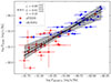 |
Fig. A.1. Monochromatic 2 keV flux densities obtained from XMM-Newton versus eROSITA data. The solid black line indicates the bisectrix. The best fit is shown by the dashed line, and 3σ uncertainties are indicated by the shaded area. Red circles and blue squares indicate whether eROSITA data come from eFEDS or eRASS1, respectively. The legend also reports the values obtained for the slope (ζ) and intercept (ξ). |
Appendix B: Flux–flux relation
Figure B.1 shows the fit of the flux–flux relation in narrow redshift bins. The best-fitting parameters of the relations are reported in Fig. 4.
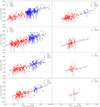 |
Fig. B.1. Fit to the X-ray–UV flux relation for the eFEDS (red circles) and eRASS1 (blue squares) samples in narrow redshift bins. The best fits are reported by dashed and dash-dotted lines, respectively. |
All Tables
All Figures
|
Fig. 1. Flux in the 0.5–2 keV band versus redshift for the source in the eFEDS (red circles) and eRASS1 (blue squares) parent samples. Given the high density of objects, contours with matching colors have been added to highlight the sources’ distributions. |
| In the text | |
|
Fig. 2. Flux in the 0.5–2 keV band versus redshift for sources in the eFEDS (red circles) and eRASS1 (blue squares) final samples. |
| In the text | |
|
Fig. 3. X-ray–UV relation. The eFEDS and eRASS1 data are shown with red circles and blue squares, respectively. The best fits for the samples are reported by the dashed and dash-dotted lines. The gray dots represent the eRASS and eFEDS parent sample, before any filtering has been applied. |
| In the text | |
|
Fig. 4. Parameters of the flux–flux relation as a function of redshift. Top: slope (γ). The gray line indicates the standard 0.6 value for the slope. Bottom: intrinsic dispersion (δ). The eFEDS and eRASS1 data are shown in blue and red, respectively. |
| In the text | |
|
Fig. 5. Hubble diagram for the simulated eRASS:4.5 sample. The density plot represents individual sources. Averaged values are indicated by black data points. The type Ia supernovae from Scolnic et al. (2018) are in light green. The solid darker green line shows the cosmographic model. |
| In the text | |
|
Fig. A.1. Monochromatic 2 keV flux densities obtained from XMM-Newton versus eROSITA data. The solid black line indicates the bisectrix. The best fit is shown by the dashed line, and 3σ uncertainties are indicated by the shaded area. Red circles and blue squares indicate whether eROSITA data come from eFEDS or eRASS1, respectively. The legend also reports the values obtained for the slope (ζ) and intercept (ξ). |
| In the text | |
|
Fig. B.1. Fit to the X-ray–UV flux relation for the eFEDS (red circles) and eRASS1 (blue squares) samples in narrow redshift bins. The best fits are reported by dashed and dash-dotted lines, respectively. |
| In the text | |
Current usage metrics show cumulative count of Article Views (full-text article views including HTML views, PDF and ePub downloads, according to the available data) and Abstracts Views on Vision4Press platform.
Data correspond to usage on the plateform after 2015. The current usage metrics is available 48-96 hours after online publication and is updated daily on week days.
Initial download of the metrics may take a while.