| Issue |
A&A
Volume 703, November 2025
|
|
|---|---|---|
| Article Number | A260 | |
| Number of page(s) | 16 | |
| Section | Planets, planetary systems, and small bodies | |
| DOI | https://doi.org/10.1051/0004-6361/202556996 | |
| Published online | 21 November 2025 | |
Precipitating electron properties of Ganymede’s aurora retrieved from Juno/UVS observations during PJ34
1
Aix-Marseille Université, CNRS, LAM,
Marseille,
France
2
Aix-Marseille Université, CNES, Institut Origines,
Marseille,
France
3
Laboratory of Atmospheric and Planetary Physics, STAR Institute, University of Liège,
Belgium
4
University of Bern, Faculty of Science, Physics Institute, Space Research & Planetary Sciences (WP),
Switzerland
5
The University of Edinburgh, School of GeoSciences,
Edinburgh,
UK
6
Centre for Exoplanet Science, University of Edinburgh,
Edinburgh,
UK
7
LATMOS/CNRS, Sorbonne Université, UVSQ,
Paris,
France
8
Department of Climate and Space Sciences and Engineering, University of Michigan,
Ann Arbor,
MI,
USA
9
Space Science and Engineering Division, Southwest Research Institute,
San Antonio,
TX,
USA
10
Physique des Interactions Ioniques et Moléculaires, CNRS et Aix-Marseille Université,
France
11
LIRA, Observatoire de Paris, Université PSL, Sorbonne Université, Université Paris Cité, CY Cergy Paris Université, CNRS,
92190
Meudon,
France
12
Univ. Grenoble Alpes, CNRS, IPAG,
38000
Grenoble,
France
13
Univ. Grenoble Alpes, CSUG,
38000
Grenoble,
France
14
Institute for Space Astrophysics and Planetology, National Institute for Astrophysics (INAF-IAPS),
Rome,
Italy
15
IRAP, CNRS-Université Paul Sabatier,
Toulouse Cedex 4,
France
16
Department of Physics and Astronomy, The University of Alabama,
Tuscaloosa,
AL
35487,
USA
17
NASA Langley Research Center,
Hampton,
Va,
USA
18
Science Systems and Applications Inc.,
Hampton,
VA,
USA
19
Space Science and Engineering Division, Southwest Research Institute,
San Antonio,
TX,
USA
★ Corresponding author: This email address is being protected from spambots. You need JavaScript enabled to view it.
Received:
26
August
2025
Accepted:
30
September
2025
Abstract
Context. Ganymede’s UV aurorae, observed by HST and Juno/UVS, trace interactions between its atmosphere and Jupiter’s magneto-sphere. These emissions, dominated by O I lines at 130.4 and 135.6 nm, are driven by electron impact on species such as H2O, O, and O2, and yet the properties of the precipitating electrons remain poorly constrained.
Aims. Our aim was to retrieve the energy and flux of precipitating electrons using UV observations from Juno/UVS during PJ34 and to assess the dominant atmospheric species producing the observed emissions.
Methods. Using the TransPlanet electron transport model and a non-local thermodynamic equilibrium (non-LTE) radiative transfer module, we simulated O I emissions for 17 auroral subregions, testing both monoenergetic and kappa-type electron distributions. The I(135.6 nm)/I(130.4 nm) line ratio was used as a diagnostic, with values varying by target species.
Results. Monoenergetic distributions fit most regions better, with mean energies of 17–300 eV and fluxes up to 2 mW m−2. Kappa and Maxwellian distributions yielded higher fluxes, but poorer spectral fits. Poor fits in some regions reflect low S/N or non-ideal electron populations.
Conclusions. Our results suggest that Ganymede’s UV aurorae are mainly driven by low- to intermediate-energy electrons. Upcoming high-resolution observations and in situ data from Juice and Europa Clipper will be key to refining these diagnostics.
Key words: plasmas / radiative transfer / planets and satellites: atmospheres / planets and satellites: aurorae
Publisher note: the original typo in the author's name Vorburger was corrected on 9 February 2026.
© The Authors 2025
 Open Access article, published by EDP Sciences, under the terms of the Creative Commons Attribution License (https://creativecommons.org/licenses/by/4.0), which permits unrestricted use, distribution, and reproduction in any medium, provided the original work is properly cited.
This article is published in open access under the Subscribe to Open model. This email address is being protected from spambots. You need JavaScript enabled to view it. to support open access publication.
1 Introduction
The interaction between a magnetosphere and a planetary atmosphere, through the magnetospheric precipitation of charged particles, leads to auroral emission phenomena. These emissions are mainly caused by precipitating electrons. When they enter the atmosphere, these electrons dissociate, excite, or ionize the atmospheric atomic and molecular species, producing light at characteristic wavelengths. In the case of Jupiter, the strength of its magnetic field and the vastness of its magnetosphere result in the brightest auroras in the Solar System, with precipitation fluxes of several tens of mW/m2 and energies of several hundred keV (Gérard et al. 2014; Benmahi et al. 2024a).
However, particles do not precipitate only in Jupiter’s polar regions. They propagate bidirectionally along magnetic field lines and also precipitate into the atmospheres of the Galilean moons orbiting the planet. This magnetosphere-satellite coupling is evidenced by specific auroral footprints associated with each moon, observed in Jupiter’s ultraviolet and infrared emissions (Connerney et al. 1993; Prangé et al. 1996; Clarke et al. 1996, 2002; Moirano et al. 2021, 2024). These electromagnetic footprints indicate current transfers and charged particle exchanges between the satellites and Jupiter’s magnetosphere (Bonfond & Zarka 2025).
Ganymede is not only the largest moon in the Solar System, it is also the only one with an intrinsic magnetic field (Gurnett et al. 1996; Kivelson et al. 1996; Williams et al. 1998; Weber et al. 2022); this field creates a mini-magnetosphere embedded within Jupiter’s larger magnetosphere. This special configuration makes Ganymede a natural laboratory for studying multi-scale interactions between magnetosphere, atmosphere, and precipitating particles.
The mechanism responsible for electron precipitation on Ganymede was recently clarified by instruments on board the Juno spacecraft, the Jovian Auroral Distributions Experiment (JADE) and Jupiter Energetic Particle Detector Instrument (JEDI) (McComas et al. 2017; Mauk et al. 2017), which detected strong downward electron fluxes and intense whistler-mode waves in the satellite’s polar regions (Clark et al. 2022; Rabia et al. 2024). Li et al. (2023) showed that these waves, depending on their propagation direction, promote the precipitation of electrons of different energies. Quasi-parallel whistler-mode waves cause the precipitation of electrons above ~1000 eV, while very oblique waves lead to the precipitation of electrons below this energy. These interactions likely explain the origin of the electrons responsible for Ganymede’s ultraviolet (UV) auroral emissions. These electrons then collide with the main atmospheric species of Ganymede: H2, H, H2O, O2, and O (Leblanc et al. 2017; Carnielli et al. 2019; Bockelée-Morvan et al. 2024; Vorburger et al. 2024).
Ultraviolet observations from the Hubble Space Telescope (Hall et al. 1995, 1998) revealed for the first time the presence of UV auroras on Ganymede, seen as UV bright ovals located in the mid-latitudes and spanning almost all longitudes. These emissions are dominated by atomic oxygen lines at 130.4 nm (a triplet transition at 130.22, 130.49, and 130.60 nm) and 135.6 nm (a doublet transition at 135.56 and 135.85 nm), corresponding to radiative transitions from the excited 3S° and 5S° states to the ground state 3P.
Excited oxygen atoms in the 3S° and 5S° states are directly produced by electron collisions with oxygen-bearing species in Ganymede’s atmosphere. Therefore, the far-ultraviolet (FUV) intensity ratio I(135.6 nm)/I(130.4 nm) of the oxygen lines is a powerful diagnostic tool. It depends not only on atmospheric density and composition, since the 130.4 nm line is partially reabsorbed by O- or H2O-rich environments, but also on the properties of the precipitating electrons, which determine the excitation efficiency of the 3S° and 5S° states. It is also influenced by atmospheric composition variation, which is controlled by sublimation of H2O in sunlit regions and by the impact of the precipitated magnetospheric plasma on species such as O2, H2, or O (Carnielli et al. 2019; Leblanc et al. 2023; Vorburger et al. 2024). A low intensity ratio (~0.2) suggests an atmosphere dominated by H2O, while a high ratio (~2.2) indicates O2 dominance with precipitated electrons from tens to hundreds of eV (Molyneux et al. 2018; Roth et al. 2021; de Kleer et al. 2023). In an atmosphere saturated with atomic oxygen, this line ratio drops to ~0.02 (de Kleer et al. 2023).
These line ratios are often quoted as fixed diagnostic values, but it is important to note that they inherently depend on the energy distribution of the precipitating electrons. Each ratio corresponds to the integral of the excitation cross sections weighted by the electron energy distribution, meaning that different shapes (e.g., Maxwellian, monoenergetic, or kappa-type distributions) can yield slightly different values for the same atmospheric composition. While previous studies have typically assumed Maxwellian electrons at 100 eV (e.g., Roth et al. 2021; de Kleer et al. 2023), for this work we explored how the choice of electron distribution affects both the resulting brightness and the line ratio (see Appendix D.3).
The main UV studies on Ganymede’s atmospheric composition (Barth et al. 1997; Hall et al. 1998; Feldman et al. 2000; Saur et al. 2015; Molyneux et al. 2018; Roth et al. 2021; Leblanc et al. 2023) have mostly relied on this line ratio to constrain early composition models. While these models account for external influences such as solar radiation on the surface, the nearby plasma-rich magnetospheric environment, which also affects the atmosphere, remains poorly constrained, as there are no in situ measurements of low-energy electrons, the main drivers of Ganymede’s auroras, at low altitudes. As noted by (Vorburger et al. 2024), deriving atmospheric densities from UV and optical emission lines is complex. One must correct for non-atmospheric contributions in the measured spectra (e.g., solar emission flux reflected by the surface), and converting observed intensities into abundances requires accurate knowledge of the photon flux in the UV range (Cessateur et al. 2012) as well as the energy spectrum of the precipitating electrons. These electrons are among the main sources of excitation for O2, O, H, and H2O, though their energy distribution varies greatly over time and location (Kivelson et al. 1996). Additionally, excitation cross section data for atomic oxygen is well known for e− + O2 → O* (Kanik et al. 2003), but limited for e− + H2O → O* (Makarov et al. 2004). In particular, the 135.6 nm emission cross section for H2O has only been directly measured at a single energy, and other studies have approximated it using different approaches, such as scaling the 130.4 nm cross section by a factor of 4 (de Kleer & Brown 2018) or adopting the single 100 eV value from Makarov et al. (2004) for 135.6 nm line (Roth et al. 2021). The lack of in situ or radio occultation data concurrent with spectroscopic observations adds another layer of complexity. A realistic model of Ganymede’s atmospheric composition therefore requires better constraints on the energy and density of precipitating electrons.
Thanks to Juno’s flyby of Ganymede at ~1000 km altitude during its 34th perijove (Hansen et al. 2022), one of the few opportunities arose to measure ambient electrons and ions near Ganymede with plasma instruments (Juno/JADE and Juno JEDI) (Allegrini et al. 2022). JADE and JEDI are mainly sensitive to electrons in the 50 eV to ~800 keV range, whereas the auroral UV emissions of Ganymede are primarily driven by lower-energy electrons (tens to hundreds of eV). Using these measurements, Vorburger et al. (2024) developed one of the most up-to-date 3D atmospheric composition models for the satellite. However, the properties of the low-energy precipitating electrons in auroral regions remain unconstrained.
Several recent studies have used coupled transport-emission models to interpret Ganymede’s auroral emissions. de Kleer et al. (2023) applied a Monte Carlo model to simulate electron populations following Maxwellian distributions, coupled with an emission model for O I lines at 630.0, 636.4, 557.7, 777.4, 844.6 nm and the UV lines at 130.4 and 135.6 nm. Their Markov Chain Monte Carlo (MCMC) approach allowed them to constrain the atmospheric composition (mostly O2) and the contribution of low-energy electrons (~35 eV) from Jupiter’s magnetosphere needed to match the observed intensities. Milby et al. (2024) extended this analysis by evaluating the sensitivity of Earth-based Keck/HIRES observations to different electron energy distributions, particularly those involving higher-energy electrons, as suggested by Saur et al. (2022). Their results indicate that the optical auroral emissions observed from Earth are not sufficient to discriminate between the canonical 100 eV electron population with a density of 70 cm−3 and the more spatially confined 200 eV distribution with a higher density of 950 cm−3 proposed by Saur et al. (2022).
Waite et al. (2024) also combined Juno Ultraviolet Spectrograph (UVS) (Davis et al. 2011) UV spectra from flyby perijoves (PJs) 34 and 35 with a transport and emission model focused on the 130.4 and 135.6 nm lines. They confirmed the O2-dominated composition and the presence of low-energy electrons (~tens of eV), with a likely energy shift toward hundreds of eV in open field regions. These works are important steps in linking line ratios to realistic electron spectra, but they rely on limited geometries (e.g., Keck/HIRES occultation for de Kleer et al. 2023’s observations) and do not yet explore the full range of auroral electron precipitation conditions on Ganymede. Our goal is to expand this modeling approach by using a multi-stream electron transport code coupled to a UV radiative transfer model, allowing spatial analysis of auroral regions at high resolution and linking the local O I line ratio I(135.6 nm)/I(130.4 nm) and total brightness to the energy distribution and flux of the precipitating electrons. Given the spectral resolution of Juno/UVS, which does not resolve O I multiplets around 130 and 135 nm, we refer in the following only to the 130.4 and 135.6 nm lines.
In this study we introduce a new approach based on fitting the O I line ratio I(135.6 nm)/I(130.4 nm) to indirectly constrain the energy and spectral shape of the precipitating electrons. For this purpose, we developed a model combining the electron transport code TransPlanet (Benmahi et al. 2024a,b; Benne et al. 2024), adapted to Ganymede’s atmospheric conditions, which simulates the production of excited atomic oxygen states 3S° and 5S°, with an auroral emission model that simulates both the 130.4 and 135.6 nm emissions and the reflection of solar flux by the surface, which contributes directly to the observed lines. By adopting an atmospheric model consistent with chemical abundances in auroral regions, this coupling allows us to simulate UV emission profiles based on different assumptions for the incident electron energy flux distributions (monoenergetic, kappa-type, or Maxwellian) and to derive expected spectral signatures in various atmospheric scenarios.
This work builds on recent studies of Ganymede’s atmosphere and its coupling with Jupiter’s magnetospheric environment. Our aim is to provide a quantitative framework for interpreting UV emissions observed around Jupiter’s icy moons, particularly Ganymede. This study also prepares for future observations by the Juice mission, whose ultraviolet instruments will offer improved spatial resolution and extended temporal coverage for studying auroral dynamics (Retherford et al. 2024). It will also support the interpretation of upcoming Europa Clipper/UVS data, contributing to the characterization of atmospheric-magnetospheric interactions at Europa.
In the next sections, we describe the numerical models used to simulate auroral zones, electron transport, and UV radiative transfer. We then present the results and compare them with existing observations. Finally, we discuss the physical implications and propose perspectives for other planetary contexts.
2 Models
2.1 Electronic transport model (TransPlanet)
Electron precipitation into Ganymede’s atmosphere was modeled using the TransPlanet code (Benmahi 2022; Benne 2023; Benmahi et al. 2024b; Benne et al. 2024), developed in collaboration with the Institut de Planétologie et d’Astrophysique de Grenoble (IPAG). This transport model originates from the Trans code, initially created by Lilensten et al. (1989) and updated by Blelly et al. (1996) to study terrestrial auroral regions. Over time, the Trans* algorithm was adapted for several solar system planets and even exoplanets (Menager 2011). This kinetic model computes the multi-stream interaction of precipitating electrons with atmospheric constituents. It has formed the core of models such as Trans-Mars (Witasse et al. 2002; Simon et al. 2009), Trans-Venus (Gronoff et al. 2007), Trans-Titan (Lilensten et al. 2005), Trans-Uranus, and more recently Trans-Jupiter (Menager et al. 2010; Benmahi 2022).
TransPlanet is a one-dimensional (1D) altitude-dependent model that enables multi-stream simulations of electron transport, including energy degradation and pitch-angle scattering, over a wide range of electron energies and incidence angles. The detailed formulation of the electron transport scheme used in this study is described in Benmahi et al. (2024a) and Benne et al. (2024). In our model, the electron transport depends on the dip-magnetic angle, which varies with the magnetic field geometry. In Ganymede’s auroral regions, this angle was computed at an altitude of 2000 km (where electrons typically begin interacting with the atmosphere) using the magnetic field model from Jia et al. (2025). Due to the low variability of this angle at that altitude, we adopted a median dip-magnetic angle of 67° calculated within the auroral regions (highlighted in yellow polygons in Fig. 1).
For this study, only magnetospheric electron precipitation was modeled. Based on a test performed with our transport model, we found that secondary electrons produced by solar UV photoionization have a flux negligible compared to precipitating magnetospheric electrons, and their contribution to the oxygen emission spectra is therefore insignificant.
Three types of incident electron energy flux distributions were used, as in Benmahi et al. (2024a,b): (1) monoenergetic distributions, (2) Maxwellian distributions, and (3) broadband kappa distributions, as defined by Coumans et al. (2002) and studied by Salveter et al. (2022) with details in Benmahi et al. (2024b). In Appendix A, we presented an example for each of these electron energy flux distributions in Fig. A.1.
To model the transport of electrons in Ganymede’s atmosphere, we used energy grids specifically tailored to each type of the precipitating electron energy flux distribution considered in the TransPlanet model. Thus, for the kappa distributions case, the energy grid was [1 eV, 100 keV], while for monoenergetic or Maxwellian distributions, the energy grids was [1 eV, β ⋅ E0], where E0 is the characteristic (or mean) energy of the distribution and β is a free parameter used to define the width of the energy grid based on the desired computational domain. For instance, in the case of a monoenergetic distribution, depending on the value of E0, there is no need for a very broad energy domain to model electron transport in the atmosphere. In contrast, for a Maxwellian distribution, a wider grid is required in our model to account for the high-energy electrons present in the right-hand tail of the distribution, since E0 represents only the peak.
The electron–matter interactions included in the transport model are both elastic and inelastic collisions with atmospheric species, as listed in Table 1. The cross sections for e−+H (Kingston & Walters 1980), e−+H2 (Muse et al. 2008), e− + O2 (Kanik et al. 2003), e− + O (Tayal & Zatsarinny 2016), and e− +H2O (Makarov et al. 2004; Roth et al. 2021) were used, covering a different energy grids depending on the electron distribution. The cross section data were lacking, power-law extrapolations were used: σ(E) ∝ E−0.65 above 400 eV (Wedde & Strand 1974), and σ(E) ∝ E−1 above 2.2 keV (Rees 1989), for both elastic and inelastic collisions. This is close to the more precise Bethe-Bloch approximation and sufficient for the energy range studied here Gronoff et al. (2025).
This study couples TransPlanet with a UV oxygen auroral emission model that accounts for e~ collisions with O2, H2O, and O. Using excitation cross sections from Kanik et al. (2003); Tayal & Zatsarinny (2016), and Makarov et al. (2004), the model calculates the volume production rates of excited atomic oxygen (O*) in the 3S° and 5Sº states. These rates feed into a radiative transfer model, linking the incident electron energy distribution to the auroral UV emissions observed.
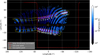 |
Fig. 1 Total brightness map of the atomic oxygen auroral emission lines around 130.4 and 135.6 nm observed during Juno’s PJ34 flyby of Ganymede. The yellow polygons (dashed lines) indicate the main auroral regions identified from the observations. The colored polygons (solid lines), magenta polygons numbered from 0 to 16, delineate the specific subregions investigated in this study. |
Inelastic electron collision reactions.
2.2 Ganymede’s atmospheric model
The atmospheric model used to simulate electron transport and radiative transfer in Ganymede’s auroral regions includes the species O2, H2O, O, H2, and H, as described in Vorburger et al. (2024). This 3D model accounts for the Jovian plasma environment and the specific photochemistry of the satellite atmosphere. In particular, it reproduces the strong dependence of the H2O density on the subsolar angle, due to the sublimation of the icy surface. The vertical abundance profiles of the other species (O2, O, H2, and H) exhibit relatively weak longitudinal and latitudinal variations compared to H2O. Among them, O2 and H2 are non-condensable species and tend to be more uniformly distributed near the surface. Atomic O and H, while highly reactive, also show relatively smooth distributions because they primarily originate from the photodissociation of O2 and H2, respectively. In the extended atmosphere, some inhomogeneities can still be observed, reflecting the influence of magnetospheric plasma precipitation (Vorburger et al. 2024).
Given that the O I line ratio 135.6 nm/130.4 nm is about 0.2 for an atmosphere dominated by H2O and about 2.2 for one dominated by O2 (de Kleer et al. 2023), and that the median observed ratio in the sunlit auroral regions (labeled 0 to 16, in Fig. 1) is 2.22, we conclude that O2 is the dominant species close to the surface at the altitudes where UV auroral emissions are produced. Therefore, to optimize modeling time, we extracted a 1D mean atmospheric profile for each chemical species within the regions outlined by the yellow polygons in Fig. 1. The vertical profiles of the main atmospheric constituents used in the electron transport and radiative transfer models are shown in Fig. 2.
The temperature profile (see Fig. 2) is taken from the atmospheric model of Carnielli et al. (2019). The initial density of thermalized electrons used in the electron transport simulations comes from the vertical profile derived by Buccino et al. (2022) based on radio occultations during the PJ34 flyby of Ganymede by the Juno spacecraft. In the absence of more accurate data, the initial electron temperature is assumed to be equal to that of the neutral gas in the TransPlanet model.
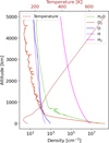 |
Fig. 2 Average vertical profiles of the densities of the main chemical species of Ganymede’s atmosphere O2, H2O, O, H2, and H in the auroral regions, outlined by the yellow polygons in Fig. 1. These profiles were directly extracted from the atmospheric model of Vorburger et al. (2024). |
2.3 Atomic oxygen UV emission model
2.3.1 Atomic oxygen UV emission lines
For this study, we developed an atomic oxygen emission model at 130.4 and 135.6 nm adapted to low-density and low-temperature atmospheres such as those of Ganymede or Europa. These atmospheres are rich in oxygen-bearing species such as H2O, O, and O2, which are the main contributors to the atomic oxygen UV emissions.
The atomic oxygen spectral lines at 130.4 nm (triplet) and 135.6 nm (doublet) result from de-excitation transitions from the excited 3S° and 5S° states to the ground state 3P, respectively (see Table 2). In this table, the factors g and J, respectively, represent the degeneracy of the lower and upper energy levels, and the rotational quantum number associated with the momentum of inertia. Aul is the Einstein coefficient representing the transition probability from the upper state u to the lower state l.
These parameters are provided by the NIST Atomic Spectra Database1.
Using the altitude-dependent production rates η3S and η5S of O* in the 3S° and 5S° states calculated by our electron transport model, and considering the Einstein coefficients Aul for each of the transitions listed in Table 2, we compute the vertical profiles of the volume emission rate (VER) for each spectral line considered in the radiative transfer model.
2.3.2 Radiative transfer model and solver adaptation
To model the auroral spectral emissions from Ganymede’s atmosphere, a cold and tenuous medium, with emission lines that may be optically thin or thick in a given direction, we developed a radiative transfer model under non-local thermodynamic equilibrium (non-LTE) conditions. For this purpose, we used the open-source solver PythonicDISORT (Ho 2024), which we adapted to our specific needs. PythonicDISORT is a one-dimensional (1D) radiative transfer solver based on the Discrete Ordinates Method (DOM), fully implemented in Python 3. It provides a modern and accessible alternative to the original FORTRAN DISORT algorithm developed by Stamnes et al. (1988). The solver is designed to simulate radiative transfer in horizontally homogeneous, plane-parallel atmospheres composed of one or more layers.
PythonicDISORT2 offers advanced functionalities for modeling radiative transfer in stratified media. It supports multi-layer atmospheres with distinct optical properties for each layer. The code supports also directional sources such as solar beams, with exponential attenuation with depth, and internal isotropic sources, such as thermal emission in LTE or non-LTE conditions. Boundary conditions of Dirichlet type can be imposed at the top and bottom of the atmosphere, with support for bidirectional reflectance distribution functions (BRDFs) to model surface reflection. Angular interpolation tools allow the precise evaluation of scattered radiation intensity along given directions, which is essential for spectral analysis and simulation of Juno/UVS observations.
The solver computes the radiative transfer equation for the spectral radiance u(τ, µ, ϕ) in a plane-parallel atmosphere at a given frequency v:
 (1)
(1)
where u(τ, µ, ϕ) is the spectral radiance in [cm−2 s−1 sr−1 Hz−1] at optical depth τ in direction (µ, ϕ). Here, µ is the cosine of the zenith angle, ϕ is the azimuthal angle (set to 0° in this study assuming azimuthally isotropic reflection), ω(τ) is the single scattering albedo, p(µ, ϕ; µ′, ϕ′) is the normalized scattering phase function, I0 is the incident beam intensity at angle (µ0, ϕ0), and S (τ) is the isotropic internal source function.
PythonicDISORT uses angular discretization based on Gauss-Legendre quadrature for zenith angles and a Fourier series expansion for azimuthal angles. The scattering phase function is expanded in Legendre polynomials, allowing an accurate representation of the medium’s scattering properties. In our radiative transfer model, we adopted a zeroth-order phase function to simulate isotropic angular scattering over 16 discrete streams. The resulting system of ordinary differential equations is solved numerically to compute the spectral radiance at each layer and direction.
The calculation of the optical depth and extinction is detailed in Appendix B.1. We have also provided details of the source function calculation in Appendix B.2.
UV transitions of atomic oxygen from the excited states 3s 3Sº and 3s 5Sº to the ground state 2p4 3P.
2.3.3 Ganymede’s surface albedo
Hall et al. (1998) estimated that the mean surface albedo of Ganymede at 135.6 nm, based on observations from the HST/STIS instrument, is approximately 2.3%. Using this value in our radiative transfer model and simulating the solar continuum between 125 nm and 150 nm, we found that this albedo does not allow for a satisfactory fit of the observed solar continuum in the various auroral regions (see Fig. 1) analyzed in this study. This discrepancy is attributed to the inhomogeneity of Ganymede’s surface, which leads to spatial variations in surface albedo (Molyneux et al. 2022).
To address this, we used our radiative transfer model to estimate the surface reflection albedo of Ganymede in the 125–150 nm spectral range for each of the 17 auroral regions (labeled 0 to 16 in Table 3), by fitting the observed emission spectra in each region. The estimated surface albedo values are listed in Table 3, along with the total brightness, emission angles, solar zenith angles (SZA), and surface albedos (SA) for each region studied.
The surface albedo values presented in Table 3 correspond to the regions specifically defined for this study (see Fig. 1). A complementary analysis of the SA over the entire sunlit face of Ganymede observed during the PJ34 flyby by the Juno spacecraft will be conducted using our atomic oxygen emission model. This future work aims to generate a spectrally resolved surface albedo map as a function of wavelength, providing a spatially resolved spectral estimate of Ganymede’s surface reflectivity.
2.3.4 Model validation (summary)
Our coupled model, which integrates electron transport, oxygen emission, and radiative transfer, was validated against three independent benchmarks. First, the modeled O I 130.4 nm triplet emissions resulting from 100 eV electron precipitation into a pure H2O atmosphere show excellent agreement with laboratory spectra from Makarov et al. (2004) (see Fig. B.1). Second, we reproduced the O I lines ratios reported by de Kleer et al. (2023) for O and O2-dominated atmospheres with less than 1% deviation, using the updated atmospheric model from Vorburger et al. (2024). Third, the radiative transfer module was bench-marked against the model of Gladstone (1992), with brightness differences below 3%. These comparisons confirm the reliability and numerical accuracy of our modeling chain. Full validation details are provided in Appendix B.3.
In the rest of this study, the modeling of O I 130.4 nm emissions includes contributions from excited O(3Sº) atoms produced by electron impact on O, O2, and H2O. However, for the 135.6 nm line, only electron collisions with O and O2 are considered as sources of O(5S°), since no reliable cross sections are currently available for electron impact on H2O producing this excited state. Consequently, the branching ratio for e + H2O leading to 135.6 nm emission could not be included in our modeling.
3 Juno/UVS observations
The Juno mission, launched in August 2011, aims to conduct an in-depth study of Jupiter and its magnetospheric environment (Bolton et al. 2017). The spacecraft was inserted into a highly elliptical polar orbit around Jupiter on July 5, 2016, and has since been performing periodic close flybys (or PJ) at an initial cadence of 53.5 days. Among these flybys, PJ34, which occurred on June 7, 2021, represented an exceptional opportunity as it included the closest approach to Ganymede by any spacecraft since Galileo. This encounter enabled a series of detailed observations of Ganymede’s immediate environment, particularly through the Ultraviolet spectrograph (UVS) on board Juno.
The UVS instrument is designed to record auroral emissions in the extreme ultraviolet (EUV) and FUV ranges, covering a spectral domain from 68 nm to 210 nm, spread over a matrix of 265 spatial × 2048 spectral channels (Davis et al. 2011; Greathouse et al. 2013; Gladstone et al. 2017; Hue et al. 2019). Its “dog-bone” shaped slit provides variable spectral resolution ranging from 1.3 to 3.0 nm depending on the position along the slit. Since Juno is spin-stabilized (with a period of about 30 s), UVS sweeps the sky once per rotation, collecting UV photons within its field of view, especially above Jupiter’s poles (Bonfond et al. 2017), and in this case from Ganymede’s atmosphere.
For this study, we used all UVS data acquired during PJ34 around Ganymede. During each 30-second spacecraft spin, UVS collects UV photons with an effective integration time of about ~ 18 ms per sky pixel through the wide parts of the slit. After data calibration reduction, each observed photon includes metadata such as spatial coordinates (latitude, longitude), detector (x, y) position, wavelength, emission angle, and more. These data were organized into three-dimensional cubes (latitude, longitude, wavelength), with a resolution of 1° in latitude and longitude and 0.1 nm in wavelength.
To improve the signal-to-noise ratio, we retained only photons collected through the two wide slits (with a spectral resolution of ~2.6 nm), while photons from the narrow slit were excluded. From these data cubes, we reconstructed maps of unabsorbed UV emission around Ganymede. These maps serve as the basis for analyzing the brightness of the O I lines at 130.4 nm and 135.6 nm, as well as for computing their intensity ratio.
In this work, we focused on modeling the UV emissions measured locally within Ganymede’s auroral regions by combining the UVS brightness data with our electron transport and radiative transfer models. This approach allows us to constrain the energy spectra of the precipitating electrons responsible for the observed emissions at a spatial resolution of about 5° in latitude and longitude.
The map of integrated emission brightness between 125 nm and 140 nm is presented in Fig. 1, where Ganymede’s auroral ovals are clearly visible, produced by atomic oxygen emissions excited during collisions between precipitating electrons and atmospheric particles.
4 Method
The objective of this study is to constrain the mean energy and energy flux of precipitating electrons in Ganymede’s auroral regions, based on the UV emission spectra observed by the Juno/UVS instrument. To enhance the signal-to-noise ratio (S/N) of the auroral emissions, we divided the sunlit auroral regions, located between 50° and −100° longitude, into 17 subregions labeled from 0 to 16 (see Fig. 1) that we have selected arbitrarily. In each of these subregions, we extracted the average auroral emission spectrum (see Fig. E.1).
We then used our TransPlanet code, coupled with our UV atomic oxygen emission model, to simulate the auroral spectra between 125 and 155 nm. The UV emission model accounts for the auroral emissions from radiative transitions of atomic oxygen at 130.4 nm (triplet from the 3S° state) and 135.6 nm (doublet from the 5S° state), as well as for the reflection of solar radiation by Ganymede’s surface, including its direct contribution to the 130.4 nm line.
The coupling between TransPlanet and the emission model proceeds as follows: the transport of precipitating electrons is modeled using TransPlanet assuming the background atmospheric composition of Vorburger et al. (2024), which provides the production rates of excited oxygen in the 3S° and 5S° states. From these rates, we compute the volume emission rates for each considered transition using the appropriate Einstein coefficients Aul (see Table 2). These volume emission rates are used as an internal source in the emission model and the radiative transfer equation is then solved for each auroral subregion, taking into account the observation geometry (emission angle, solar zenith angle), atmospheric composition, and surface albedo. The resulting synthetic spectrum is finally convolved with the Juno/UVS instrumental spectral resolution (about 2.6 nm) to allow direct comparison with the observations. As input to the TransPlanet model, we consider a precipitating electron energy flux distribution (monoenergetic, Maxwellian, or kappa-shaped) defined by two parameters: the mean energy 〈E〉 (in eV) and the energy flux ψ (in mW/m2).
First, we tested the influence of each of these two parameters independently on the modeled spectra. We confirmed that both the total brightness and the intensity ratio of the O I lines depend on 〈E〉 and ψ. Therefore, in a second step, we performed a two-dimensional fitting of the observed spectrum by exploring a parameter grid [〉E〉, ψ] spanning a wide range of conditions. For monoenergetic and Maxwellian electrons, we used: ψ = [0.05, 0.1, 0.2, 0.5, 1.0, 2.0, 5.0, 10.0, 50.0] mW/m2 and 〈E〉 = [14, 17, 20, 30, 50, 70, 100, 120, 150, 200, 250, 300] eV. The lower bound of the 〈E〉 grid corresponds to the minimum excitation threshold for producing O* atoms in the 3S° and 5S° states via electron impact on the atmospheric particles. The upper bound is set just above the energy (~250 eV) at which monoenergetic electrons interact weakly with the atmosphere and deposit most of their energy into the satellite’s surface.
For the kappa distribution, we used: 〈E〉 = [10, 20, 50, 100, 200, 300, 500, 700, 1000, 1500, 2000, 2500] eV, with the same ψ grid as in the monoenergetic case. Since the kappa distribution is a continuous function, we discretized it in our electron transport model over an energy range from 1 eV to 100 keV, for each value of the mean energy 〈E〉 considered in the fitting grid. -In the same way, for the case of Maxwellian distributions, we also discretize it in an energy range from 1 eV to 2〈E〉.
Finally, for each auroral subregion, we modeled a set of auroral spectra covering all combinations of [〈E〉, ψ] for all types of distributions. For each parameter pair, we computed the reduced χ2, the intensity ratio of the O I 135.6/130.4 nm lines, and their total brightness in Rayleigh (R). We then built three likelihood maps  , one for the kappa distribution, one for the monoenergetic distribution, and one for the Maxwellian distribution. The maximum of this likelihood function thus identifies the optimal pair [〈E〉, ψ] corresponding to the best fit to the observed spectrum in each analyzed region, which then allows us to estimate the energy flux and the mean energy of the precipitating electron in a given auroral subregion.
5 Results and discussion
We now present the results obtained in this study, aimed at characterizing the properties of precipitating electrons responsible for the auroral UV emissions observed at Ganymede. As an example, we first focus on region 7. The resulting likelihood maps are presented in Fig. C.1, illustrating for monoenergetic or kappa case the explored pairs of [〈E〉, ψ]. On these maps, the green star indicates the global maximum likelihood, representing the parameter set that provides the best fit to the observed spectrum based on the minimal reduced χ2 criterion.
Although these maps exhibit several local maxima, as discussed in detail in Appendix C, we systematically retained the primary mode corresponding to the global minimum of the reduced χ2 to extract the fitted spectra. Fig. C.2 illustrates that the secondary modes, although sometimes close to the global maximum in terms of likelihood, do not yield satisfactory fits. For the case of the Maxwellian distribution, the likelihood map in the parameter space [〈E〉, ψ] (not shown here) behaves exactly as in the monoenergetic and kappa cases, and only the parameter pair [〈E〉, ψ] corresponding to the maximum likelihood provides the best-fitting solution.
It is noteworthy that these local maxima particularly appear in regions of high mean energy and high flux. However, extending the parameter grid in these directions would lead to excessively high estimates of precipitated flux, inconsistent with in situ observations. Indeed, in situ measurements by Ebert et al. (2022) from the JADE and JEDI instruments on board Juno during the PJ34 flyby revealed precipitating electrons with energies up to 3 keV and a total energy flux of about 10 mW/m2 in Ganymede’s auroral regions. These observations support the consistency of the upper limits adopted in our parameter space with direct measurements. Therefore, we deliberately limited our parameter exploration to physically plausible values compatible with available observational constraints.
The observed spectrum in region 7 and its best fits for the three considered distributions are presented in Fig. 3. In this case, the modeled spectrum corresponding to the best fit for the monoenergetic distribution, plotted in blue in Fig. 3, has a line  and a total brightness B = 297.25 R for the combined 130.4 and 135.6 nm lines. The estimated parameters, mean energy and precipitation energy flux is (17 ± 1) eV and (1 ± 0.3) mW/m2 respectively, with a reduced χ2 of 1.9. The 1-σ uncertainties were obtained by locally fitting the main peak of the likelihood map with a two-dimensional Gaussian function. Conversely, for the kappa or the Maxwellian distributions, the likelihood map exhibits significant spreading along the mean energy axis around the global maximum, leading to larger uncertainty in the estimation of this parameter.
Spectral fitting results obtained for all 17 regions are presented in Fig. E.1 and summarized in Table 4. In this table, the columns show the best fits for the parameters 〈E〉 and ψ obtained by considering a monoenergetic, a Maxwellian, and a kappa distribution of the precipitated electron flux. The 1-σ uncertainties values for 〈E〉 and ψ are given in the brackets.
We observe that for several regions (particularly regions 2, 3, 4, 15, and 16), the monoenergetic, the Maxwellian, nor the kappa distributions provide satisfactory fits to the observed spectra. In most of these cases, the poor fitting quality can results from a low signal-to-noise ratio, especially evident in region 8, which compromises the reliable estimation of mean electron energy and energy flux. However, another possibility is that the precipitating electrons in these regions do not follow the idealized distribution types assumed in our electron transport model. More complex or mixed electron populations, not accounted for here, could better explain the observed spectral characteristics.
We also observe that in all regions from 0 to 16, the best-fit spectra obtained using either a Maxwellian or a kappa distribution are very similar. Although the retrieved parameters 〈E〉 and ψ differ significantly between these two distribution types, the resemblance in the modeled spectra arises from the fact that both distributions are similar at low energies. Given the energy ranges considered in this study, this outcome was expected.
In some regions (e.g., regions 6, 9, 10, and 11), all distribution types provide satisfactory fits to the observed spectra. However, the derived values of mean energy and energy flux differ significantly depending on the distribution type used, emphasizing the importance of choosing the appropriate model for physical interpretation. Conversely, in cases like region 5, although the monoenergetic distribution provides the best fit, the extracted parameters remain consistent with those derived from the kappa distribution. To further discriminate the most appropriate model in such regions, we computed the Bayesian information criterion (BIC)3 for each spectral fit across all regions (see Fig. E.1). This criterion is defined as
 (2)
(2)
where k is the number of parameters (in our case we have two fit parameters for each distribution), N is the size of the spectral sample, and  is the maximum of the likelihood. The BIC is consistently lowest for the monoenergetic case in these regions, supporting it as the most ideal choice for retrieving the electron energy and energy flux.
In comparison to the recent study by Waite et al. (2024), our results offer complementary insights into the electron precipitation processes in Ganymede’s auroral regions. Waite et al. (2024) used in situ observations from Juno/JADE at the reconnection boundary to directly constrain the precipitating electron energy spectrum, adopting a unidirectional transport model with secondary electron production to reproduce the observed UV emissions. Their modeling favors relatively energetic electron populations (e.g., fluxes up to 9 mW/m2) and suggests that the column density of O2 required to explain the observed brightness is significantly larger (~4.5×10 cm−2) than previously assumed. In contrast, our approach uses spectral fitting of UVS observations to retrieve the best-fit parameters of idealized electron distributions (monoenergetic, Maxwellian, and kappa) in 17 distinct regions. Despite the different methodologies, the range of energy fluxes retrieved in our study (typically 0.1−2 mW/m2) is consistent with the values observed in the polar cap by JADE (0.5–1.7 mW/m2), and overlaps with the lower end of the reconnection-associated fluxes reported by Waite et al. (2024). Notably, Waite et al. argue that Maxwellian or even kappa distributions may not be physically realistic in Ganymede’s thin atmosphere due to strong rovibrational cooling, which limits the formation of thermalized electron populations. While our retrievals often favor monoenergetic fits, Maxwellian or kappa distributions can still approximate the observations in some cases. However, we acknowledge that these are idealized cases and may not fully capture the complexity of the precipitating electron populations shaped by Ganymede’s magnetospheric dynamics. Future modeling efforts incorporating the measured JADE spectra directly as input, as done by Waite et al. (2024), will be essential to further refine our understanding of electron-driven emissions at Ganymede.
To complement the individual subregion analysis, we performed spectral fits over two broader composite regions (yellow polygons) covering the entire sunlit auroral zones in the northern and southern hemispheres, respectively. In both cases, monoenergetic distributions provided the best spectral fit based on the BIC criterion. In the northern hemisphere, the retrieved mean energy is 20 ± 3 eV with an energy flux of 0.5 ± 0.19 mW/m2, consistent with typical values derived from the smaller subregions. In contrast, the southern hemisphere yields a lower mean energy of 14 ± 1 eV but a significantly higher energy flux of 50.0 ± 3.84 mW/m2, which, while unusually large compared to its northern counterpart, is still within the range of the in situ measurements (Ebert et al. 2022). Although these values represent spatial averages, caution is warranted when interpreting them physically, as the solar zenith and emission angles vary substantially across these broad regions. In fact, a sensitivity test (figures not shown here) conducted for Region 7 shows that both the modeled line ratio and total brightness can vary significantly when either the solar zenith angle or the emission angle is varied between 0° and 80°, which corresponds roughly to the range of variation of the emission angle and SZA in theses broader auroral regions, highlighting the importance of accounting for local observational geometry to avoid potential biases in the retrieved electron properties.
Greathouse et al. (2022) and previous modeling work (e.g., Eviatar et al. 2001; Jia et al. 2009; Duling et al. 2014) suggest that the location of the polar-most boundary of the auroral curtain corresponds to the position of Ganymede’s last closed field lines. Greathouse et al. (2022) also demonstrated that diffuse auroral emissions extend equatorward of the auroral curtain, indicating that electron precipitation occurs throughout the closed field line region on the leading side of Ganymede facing the magnetospheric plasma flow. In contrast, our study focuses on integrated regions to maximize the signal-to-noise ratio of the oxygen emissions, and is therefore more representative of electron precipitation at the open-closed field line boundary.
Saur et al. (2022) applied the method developed by Eviatar et al. (2001) to estimate the properties of precipitating electrons from the observed brightness of the O I 135.6 nm emission in Ganymede’s brightest auroral regions. Assuming a Maxwellian distribution, they inferred mean electron energies of about 200 eV and energy fluxes between 10 and 100 mW/m2 to match the observed brightness. In our study, using a radiative transfer model that simultaneously fits both the O I 130.4 nm and 135.6 nm lines, we retrieved electron energies ranging from 20 to 300 eV for the 17 sunlit auroral subregions. These values are in good agreement with the energy estimates of Saur et al. (2022). However, the energy fluxes we derived, typically between 0.1 and 2 mW/m2 for monoenergetic distributions, are lower than their range of derived fluxes. This discrepancy likely arises from the fact that our model applies stronger constraints by fitting both lines simultaneously, which makes it more sensitive to the spectral shape of the electron energy distribution. In most regions, monoenergetic distributions provide the best spectral fits, particularly where the S/N is highest. In lower S/N regions, Maxwellian distributions may occasionally yield comparable fits, but this likely reflects fitting degeneracies rather than a physical preference for a Maxwellian shape. All three distributions considered here are idealized approximations, and the actual precipitating electron populations may follow more complex shapes, for instance, a combination of two Maxwellians, or a kappa distribution with an additional peak as suggested by Juno/JEDI in situ measurements in Jupiter’s magnetosphere (e.g., Mauk et al. 2017; Salveter et al. 2022).
In addition, while the BIC helps to identify the best-fitting distribution in each region, the values as derived considering the monoenergetic and Maxwellian distribution are, in bright regions such as 6, 9, 10, and 11, comparable. For example, in regions 6 and 10, the Maxwellian distribution yields mean energies of 200–250 eV and energy fluxes around 5 mW/m2, which are in good agreement with the estimates from Saur et al. (2022). These results illustrate that although monoenergetic distributions provide the best fits in most cases, Maxwellian distributions can still be consistent with the observations in several regions.
Generally, the energy fluxes derived from our analysis are lower than those typically measured in Jupiter’s main auroral regions, where fluxes range from 5 to 100 mW/m2 (Benmahi et al. 2024b). They are also lower than the average precipitating flux estimated from in situ measurements by Ebert et al. (2022) during PJ34, which reported total energy fluxes of precipitating electrons reaching up to 10 mW/m2 in Ganymede’s auroral regions. Similarly, Waite et al. (2024) estimated electron fluxes precipitating onto Ganymede’s atmosphere around 9 to 10 mW/m2, for electrons extending up to a few MeV. This lower energy flux estimates are entirely logical since they represent only the portion of electrons precipitating from the Jovian magnetosphere with energies sufficient to produce auroral emissions. Electrons with higher energies (beyond a few hundred eV) are not responsible for auroral emissions, as they are directly impacting the surface and do not efficiently contribute to UV emissions. This behavior is consistent with the known excitation cross sections of oxygen species, which decrease rapidly with increasing electron energy following a power-law dependence (Kanik et al. 2003; Makarov et al. 2004; Tayal & Zatsarinny 2016; Roth et al. 2021). Also, measurements by Galileo during flybys G1, G8, and G28 allowed Liuzzo et al. (2020) to estimate electron fluxes in polar regions of Ganymede between 4.5 keV and 100 MeV at about 5 mW/m2, consistent with our estimates focused on the lower-energy electron portion responsible for UV emissions. As a result, matching the observed UV brightness with high-energy electrons would require unrealistically large precipitation fluxes in our model, inconsistent with current in situ constraints around Ganymede (Frank et al. 1997; Ebert et al. 2022). Our diagnostic method is therefore most sensitive to lower-energy electrons, while higher-energy electrons pass through the atmosphere with minimal interaction.
In this study, we used a kappa distribution (Coumans et al. 2002) (see example in Fig. A.1) with a fixed parameter κ = 2.5 (see Equation (D.1)), assuming that electrons following this kappa distribution and precipitating onto Ganymede follow a similar distribution to those observed in the Jovian environment. However, this hypothesis warrants caution. Indeed, several studies (Salveter et al. 2022; Benmahi et al. 2024b) indicate that the κ parameter can vary slightly within the magnetosphere, potentially affecting the shape of the energy distribution in precipitation regions. Benmahi et al. (2024b) notably demonstrated for Jupiter that variability in κ significantly influences the volume emission rates of H2. This influence on the volume emission rate arises from the fact that variations in the parameter κ affect the slope of the electron energy distribution at higher energies. By analogy, a similar effect is expected for atomic oxygen emissions at Ganymede. We therefore performed a sensitivity analysis of the κ parameter and its impact on O I emissions in Ganymede’s auroral regions (see Appendix D.3). We find that small variations around κ = 2.5 (approximately 2.1–3.0) have little effect on the line ratio  , but they significantly affect the total line brightness, consistent with Benmahi et al. (2024b). As a perspective, beyond the scope of this study, tighter observational constraints on κ in Ganymede’s immediate environment, leveraging in situ measurements from Juno/JADE and Juno/JEDI, could substantially refine the diagnostics presented here.
Beyond the distributions, energies, and energy fluxes of precipitating electrons, other model parameters can also influence spectral interpretation, particularly those related to atmospheric composition and to the interactions of electrons with Ganymede’s surface. To evaluate the influence of atmospheric composition on the atomic oxygen line ratio at 130.4 and 135.6 nm, we conducted a sensitivity study centered on the H2O molecule (see Appendix D.1). As illustrated in Fig. D.2, the abundance of H2O significantly affects the line ratio only when it is increased by a factor of more than 5 compared to the initial abundance estimated by Vorburger et al. (2024). This corresponds to local H2O densities comparable to or greater than those of O2 in auroral regions far from the subsolar point, a configuration considered unrealistic according to current atmospheric models of Ganymede (Carnielli et al. 2019; Leblanc et al. 2023; Bockelée-Morvan et al. 2024; Vorburger et al. 2024). These results suggest that line ratio diagnostics are promising for constraining oxygen species abundances, but require high spectral and spatial resolution and good S/N. These conditions may be met by Juice-UVS during the Ganymede orbital phase, enabling refined compositional analysis.
Another parameter that could have an impact on the oxygen line ratio is the precipitating electrons “albedo” at Ganymede’s surface. For this study, we performed a dedicated sensitivity analysis (see Appendix D.2). The preliminary results shows that a surface reflection of 10 to 20% of the precipitating electrons starts to significantly impact brightness and line ratios (respectively, by a factors ~2 and ~1.3 beyond 60% of the precipitating electrons “albedo”) of atomic oxygen emissions in the satellite’s atmosphere (see Fig. D.3). As a precaution, we set the surface albedo to 0% in the TransPlanet model for this study. This hypothesis does not affect our primary conclusions; however, a complementary study is underway, based on a Geant4-like library modeling with laboratory experiments, aiming at better constraining this albedo value, particularly as a function of the incident electron energy, to strengthen the robustness of our model.
In summary, this study provides the first quantitative constraint on the properties of precipitating electrons responsible for the auroral UV emissions at Ganymede. The results highlight the complexity of magnetosphere-atmosphere coupling in this environment, while highlighting the need for complementary observations and refined models to better characterize the physical processes involved.
 |
Fig. 3 Top: UVS spectrum observed in region 7 (in gray). The blue, red, and green spectra are respectively the best fits obtained by considering a monoenergetic distribution, a Maxwellian distribution, and a kappa distribution. The estimated parameters [〈E〉, ψ] obtained from these fits with our model are shown in the legend. Bottom: residuals of the best fit for each type of electron energy flux distribution. For each distribution type, this residual is calculated by subtracting the best fit from the observed spectrum. |
Summary of results obtained for each auroral subregion.
6 Conclusions
In this study, we presented the first quantitative characterization of the energy and energy flux of precipitating electrons responsible for Ganymede’s UV auroral emissions, based on Juno/UVS observations and a modeling framework coupling the Trans-Planet electron transport model with a non-LTE radiative transfer model for UV atomic oxygen emissions.
A total of 17 sunlit auroral subregions were analyzed. For each, we computed best-fit solutions assuming monoenergetic, Maxwellian, and kappa-type electron energy flux distributions, by exploring a parameter space [〈E〉, ψ] and selecting the pair maximizing the likelihood function. The resulting best fits successfully reproduce the spectral shape and intensity of the 130.4 and 135.6 nm oxygen lines in most regions, with reduced χ2 values generally below 2. Our results show that the inferred mean energies of the precipitating electrons range between 17 and 300 eV, with a median value of  eV in most regions. The energy fluxes derived from the fits vary between 0.1 and ~2 mW/m2 with a median value
  mW/m2. These values are consistent with previous in situ estimates around Ganymede (Liuzzo et al. 2020; Mauk et al. 2020) (Ebert et al. 2022), and are significantly lower than those observed in Jupiter’s main auroral regions.
In some regions (e.g., 2, 3, 4, 15, 16), none of the distributions provides a good fit, likely due to low signal-to-noise ratios, unmodeled atmospheric effects, or non-ideal electron populations not assumed in our electron transport model.
Conversely, regions 0, 7, and 13 exhibit excellent agreement between the modeled and observed spectra, with well-constrained energy and flux values. In particular, region 7 shows the highest brightness (over 300 R) and a line ratio of 2.72, best reproduced by a monoenergetic distribution with 〈E〉 = 17 eV and ψ = 1 mW/m2.
The sensitivity studies conducted on atmospheric H2O abundances, the electron surface albedo, and the kappa parameter variabilities demonstrate the following: (1) The line ratio I(135.6 nm)/I(130.4 nm) is affected by H2O only if its abundance is increased by a factor of more than 5 relative to current atmospheric models, and (2) the reflection of more than 10–20% of precipitating electrons at the surface could significantly impact the UV brightness and line ratio. These results justify our assumptions of moderate H2O density and zero surface albedo for reflected electrons. (3) The κ parameter strongly influences the total brightness of oxygen emissions, although its impact on the line ratio remains limited for moderate variations around κ = 2.5. This confirms the role of the suprathermal tail in shaping auroral outputs and suggests that better constraints on κ, particularly through in situ measurements by Juno/JADE, Juno/JEDI, or Juice/PEP, could refine the retrievals of precipitating electron populations.
Overall, our analysis confirms that Ganymede’s UV auroral emissions are mainly produced by low- to intermediate-energy electrons (14–300 eV), with moderate energy fluxes (<2 mW/m2), and our BIC calculations indicate that the monoenergetic distribution provides better fits in most well-observed regions.
Further progress will require better observational constraints on the local atmospheric composition, more accurate modeling of electron-surface interactions, and high-resolution spectroimaging data from upcoming missions such as Juice and Europa Clipper, which will enable a more complete understanding of the electron precipitation processes and their coupling to Ganymede’s unique magnetospheric environment.
Acknowledgements
B. Benmahi and V. Hue acknowledge support from the French government under the France 2030 investment plan, as part of the Initiative d’Excellence d’Aix-Marseille Université – A*MIDEX AMX-22-CPJ-04. French authors acknowledge the support of CNES to the Juno and Juice missions. This work was supported by the Fonds de la Recherche Scientifique – FNRS under Grant(s) No. T003524F. B. Bonfond is a Research Associate of the Fonds de la Recherche Scientifique – FNRS.
References
- Allegrini, F., Bagepal, F., Ebert, R. W., et al. 2022, Geophys. Res. Lett., 49, e2022GL098682 [Google Scholar]
- Barth, C. A., Hord, C. W., Stewart, A. I. F., et al. 1997, Geophys. Res. Lett., 24, 2147 [NASA ADS] [CrossRef] [Google Scholar]
- Benmahi, B. 2022, PhD thesis, Université de Bordeaux [Google Scholar]
- Benmahi, B., Bonfond, B., Benne, B., et al. 2024a, A&A, 685, A26 [Google Scholar]
- Benmahi, B., Bonfond, B., Benne, B., et al. 2024b, A&A, 691, A91 [NASA ADS] [CrossRef] [EDP Sciences] [Google Scholar]
- Benne, B. 2023, PhD thesis, Université de Bordeaux [Google Scholar]
- Benne, B., Benmahi, B., Dobrijevic, M., et al. 2024, A&A, 686, A22 [NASA ADS] [CrossRef] [EDP Sciences] [Google Scholar]
- Blelly, P. L., Robineau, A., & Alcayde, D. 1996, J. Atmos. Terrestr. Phys., 58, 273 [Google Scholar]
- Bockelée-Morvan, D., Lellouch, E., Poch, O., et al. 2024, A&A, 681, A27 [NASA ADS] [CrossRef] [EDP Sciences] [Google Scholar]
- Bolton, S. J., Adriani, A., Adumitroaie, V., et al. 2017, Science, 356, 821 [Google Scholar]
- Bonfond, B., & Zarka, P. 2025, Electrodynamic Coupling between Ganymede and the Jovian Ionosphere (Cambridge University Press) [Google Scholar]
- Bonfond, B., Gladstone, G. R., Grodent, D., et al. 2017, Geophys. Res. Lett., 44, 4463 [NASA ADS] [CrossRef] [Google Scholar]
- Buccino, D. R., Parisi, M., Gramigna, E., et al. 2022, Geophys. Res. Lett., 49, e2022GL098420 [Google Scholar]
- Carnielli, G., Galand, M., Leblanc, F., et al. 2019, Icarus, 330, 42 [Google Scholar]
- Cessateur, G., Lilensten, J., Barthélémy, M., et al. 2012, Icarus, 218, 308 [Google Scholar]
- Clark, G., Kollmann, P., Mauk, B. H., et al. 2022, Geophys. Res. Lett., 49, e2022GL098572 [Google Scholar]
- Clarke, J. T., Ballester, G. E., Trauger, J., et al. 1996, Science, 274, 404 [Google Scholar]
- Clarke, J. T., Ajello, J., Ballester, G., et al. 2002, Nature, 415, 997 [NASA ADS] [CrossRef] [Google Scholar]
- Connerney, J. E. P., Baron, R., Satoh, T., & Owen, T. 1993, Science, 262, 1035 [NASA ADS] [CrossRef] [Google Scholar]
- Coumans, V., Gérard, J.-C., Hubert, B., & Evans, D. S. 2002, J. Geophys. Res.: Space Phys., 107, SIA5 [Google Scholar]
- Davis, M. W., Gladstone, G. R., Greathouse, T. K., et al. 2011, in Radiometric Performance Results of the Juno Ultraviolet Spectrograph (Juno/UVS), eds. H. A. MacEwen, & J. B. Breckinridge (San Diego, California, USA), 814604 [Google Scholar]
- de Kleer, K., & Brown, M. E. 2018, AJ, 156 [Google Scholar]
- de Kleer, K., Milby, Z., Schmidt, C., Camarca, M., & Brown, M. E. 2023, Planet. Sci. J., 4, 37 [NASA ADS] [CrossRef] [Google Scholar]
- Drouin, D., Couture, A. R., Joly, D., et al. 2007, Scanning, 29, 92 [CrossRef] [PubMed] [Google Scholar]
- Duling, S., Saur, J., & Wicht, J. 2014, J. Geophys. Res.: Space Phys., 119, 4412 [Google Scholar]
- Ebert, R. W., Fuselier, S. A., Allegrini, F., et al. 2022, Geophys. Res. Lett., 49, e2022GL099775 [Google Scholar]
- Eviatar, A., Strobel, D. F., Wolven, B. C., et al. 2001, ApJ, 555, 1013 [NASA ADS] [CrossRef] [Google Scholar]
- Feldman, P. D., McGrath, M. A., Strobel, D. F., et al. 2000, ApJ, 535, 1085 [NASA ADS] [CrossRef] [Google Scholar]
- Frank, L. A., Paterson, W. R., Ackerson, K. L., & Bolton, S. J. 1997, Geophys. Res. Lett., 24, 2159 [Google Scholar]
- Gladstone, G. R. 1992, J. Geophys. Res.: Space Phys., 97, 19519 [Google Scholar]
- Gladstone, G. R., Persyn, S. C., Eterno, J. S., et al. 2017, Space Sci. Rev., 213, 447 [Google Scholar]
- Greathouse, T. K., Gladstone, G. R., Davis, M. W., et al. 2013, in UV, X-Ray, and Gamma-Ray Space Instrumentation for Astronomy XVIII, 8859 (SPIE), 216 [Google Scholar]
- Greathouse, T. K., Gladstone, G. R., Molyneux, P. M., et al. 2022, Geophys. Res. Lett., 49, e2022GL099794 [Google Scholar]
- Gronoff, G., Lilensten, J., Simon, C., et al. 2007, A&A, 465, 641 [NASA ADS] [CrossRef] [EDP Sciences] [Google Scholar]
- Gronoff, G., Simon Wedlund, C., Hegyi, B., et al. 2025, Adv. Space Res., 75, 8232 [Google Scholar]
- Gurnett, D. A., Kurth, W. S., Roux, A., Bolton, S. J., & Kennel, C. F. 1996, Nature, 384, 535 [Google Scholar]
- Gérard, J.-C., Bonfond, B., Grodent, D., et al. 2014, J. Geophys. Res.: Space Phys., 119, 9072 [CrossRef] [Google Scholar]
- Hall, D. T., Strobel, D. F., Feldman, P. D., McGrath, M. A., & Weaver, H. A. 1995, Nature, 373, 677 [Google Scholar]
- Hall, D. T., Feldman, P. D., McGrath, M. A., & Strobel, D. F. 1998, ApJ, 499, 475 [NASA ADS] [CrossRef] [Google Scholar]
- Hansen, C. J., Bolton, S., Sulaiman, A. H., et al. 2022, Geophys. Res. Lett., 49, e2022GL099285 [Google Scholar]
- Ho, D. J. 2024, J. Open Source Softw., 9, 6442 [Google Scholar]
- Hue, V., Gladstone, G. R., Greathouse, T. K., et al. 2019, AJ, 157, 90 [NASA ADS] [CrossRef] [Google Scholar]
- Jia, X., Walker, R. J., Kivelson, M. G., Khurana, K. K., & Linker, J. A. 2009, J. Geophys. Res.: Space Phys., 114 [Google Scholar]
- Jia, X., Kivelson, M. G., Khurana, K. K., & Walker, R. J. 2025, J. Geophys. Res.: Planets, 130, e2024JE008309 [Google Scholar]
- Kanik, I., Noren, C., Makarov, O. P., et al. 2003, J. Geophys. Res.: Planets, 108 [Google Scholar]
- Kingston, A. E., & Walters, H. R. J. 1980, J. Phys. B: At. Mol. Phys., 13, 4633 [NASA ADS] [CrossRef] [Google Scholar]
- Kivelson, M. G., Khurana, K. K., Russell, C. T., et al. 1996, Nature, 384, 537 [NASA ADS] [CrossRef] [Google Scholar]
- Leblanc, F., Oza, A. V., Leclercq, L., et al. 2017, Icarus, 293, 185 [NASA ADS] [CrossRef] [Google Scholar]
- Leblanc, F., Roth, L., Chaufray, J. Y., et al. 2023, Icarus, 399, 115557 [NASA ADS] [CrossRef] [Google Scholar]
- Li, W., Ma, Q., Shen, X.-C., et al. 2023, Geophys. Res. Lett., 50, e2022GL101555 [Google Scholar]
- Lilensten, J., Kofman, W., Wisemberg, J., Oran, E. S., & DeVore, C. R. 1989, Ann. Geophys., 7, 83 [NASA ADS] [Google Scholar]
- Lilensten, J., Simon, C., Witasse, O., et al. 2005, Icarus, 174, 285 [NASA ADS] [CrossRef] [Google Scholar]
- Liuzzo, L., Poppe, A. R., Paranicas, C., et al. 2020, J. Geophys. Res.: Space Phys., 125, e2020JA028347 [Google Scholar]
- Makarov, O. P., Ajello, J. M., Vattipalle, P., et al. 2004, J. Geophys. Res.: Space Phys., 109 [Google Scholar]
- Mauk, B. H., Haggerty, D. K., Paranicas, C., et al. 2017, Nature, 549, 66 [NASA ADS] [CrossRef] [Google Scholar]
- Mauk, B. H., Clark, G., Allegrini, F., et al. 2020, J. Geophys. Res.: Space Phys., 125, e2020JA027964 [Google Scholar]
- McComas, D. J., Alexander, N., Allegrini, F., et al. 2017, Space Sci. Rev., 213, 547 [Google Scholar]
- Menager, H. 2011, PhD thesis, Laboratoire de Planétologie de Grenoble [Google Scholar]
- Menager, H., Barthélemy, M., & Lilensten, J. 2010, A&A, 509, A56 [NASA ADS] [CrossRef] [EDP Sciences] [Google Scholar]
- Milby, Z., Kleer, K. d., Schmidt, C., & Leblanc, F. 2024, Planet. Sci. J., 5, 153 [NASA ADS] [CrossRef] [Google Scholar]
- Moirano, A., Mura, A., Adriani, A., et al. 2021, J. Geophys. Res.: Space Phys., 126, e2021JA029450 [Google Scholar]
- Moirano, A., Mura, A., Hue, V., et al. 2024, J. Geophys. Res.: Planets, 129, e2023JE008130 [Google Scholar]
- Molyneux, P. M., Nichols, J. D., Bannister, N. P., et al. 2018, J. Geophys. Res.: Space Phys., 123, 3777 [Google Scholar]
- Molyneux, P. M., Greathouse, T. K., Gladstone, G. R., et al. 2022, Geophys. Res. Lett., 49, e2022GL099532 [Google Scholar]
- Muse, J., Silva, H., Lopes, M. C. A., & Khakoo, M. A. 2008, J. Phys. B: At. Mol. Opt. Phys., 41, 095203 [NASA ADS] [CrossRef] [Google Scholar]
- Prangé, R., Rego, D., Southwood, D., et al. 1996, Nature, 379, 323 [CrossRef] [Google Scholar]
- Rabia, J., Hue, V., André, N., et al. 2024, J. Geophys. Res.: Space Phys., 129, e2024JA032604 [Google Scholar]
- Rees, M. H. 1989, Physics and Chemistry of the Upper Atmosphere (Cambridge University Press) [Google Scholar]
- Retherford, K. D., Becker, T. M., Gladstone, G. R., et al. 2024, Space Sci. Rev., 220, 89 [Google Scholar]
- Roth, L., Ivchenko, N., Gladstone, G. R., et al. 2021, Nat. Astron., 5, 1043 [NASA ADS] [CrossRef] [Google Scholar]
- Salveter, A., Saur, J., Clark, G., & Mauk, B. H. 2022, J. Geophys. Res.: Space Phys., 127, e2021JA030224 [CrossRef] [Google Scholar]
- Saur, J., Duling, S., Roth, L., et al. 2015, J. Geophys. Res.: Space Phys., 120, 1715 [NASA ADS] [CrossRef] [Google Scholar]
- Saur, J., Duling, S., Wennmacher, A., et al. 2022, Geophys. Res. Lett., 49, e2022GL098600 [Google Scholar]
- Simon, C., Witasse, O., Leblanc, F., Gronoff, G., & Bertaux, J. L. 2009, Planet. Space Sci., 57, 1008 [NASA ADS] [CrossRef] [Google Scholar]
- Stamnes, K., Tsay, S.-C., Wiscombe, W., & Jayaweera, K. 1988, Appl. Opt., AO, 27, 2502 [Google Scholar]
- Tayal, S. S., & Zatsarinny, O. 2016, Phys. Rev. A, 94, 042707 [NASA ADS] [CrossRef] [Google Scholar]
- Vorburger, A., Fatemi, S., Carberry Mogan, S. R., et al. 2024, Icarus, 409, 115847 [NASA ADS] [CrossRef] [Google Scholar]
- Waite, J. H., Greathouse, T. K., Carberry Mogan, S. R., et al. 2024, J. Geophys. Res.: Planets, 129, e2023JE007859 [Google Scholar]
- Weber, T., Moore, K., Connerney, J., et al. 2022, Geophys. Res. Lett., 49, e2022GL098633 [Google Scholar]
- Wedde, T., & Strand, T. G. 1974, J. Phys. B: At. Mol. Phys., 7, 1091 [NASA ADS] [CrossRef] [Google Scholar]
- Williams, D. J., Mauk, B., & McEntire, R. W. 1998, J. Geophys. Res.: Space Phys., 103, 17523 [Google Scholar]
- Witasse, O., Dutuit, O., Lilensten, J., et al. 2002, Geophys. Res. Lett., 29, 104 [CrossRef] [Google Scholar]
The package is available at: https://github.com/LDEO-CREW/Pythonic-DISORT, and its documentation (including Jupyter note-books) is accessible at: https://pythonic-disort.readthedocs.io/en/latest/
The BIC is a model selection criterion that penalizes models with many parameters to avoid overfitting. Lower BIC values indicate a better balance between model complexity and fit quality.
Appendix A Illustrative example of electron energy distributions
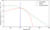 |
Fig. A.1 Three electron energy flux distributions with the same mean energy (100 eV) and energy flux (1 mW/m2): monoenergetic (blue), Maxwellian (red), and kappa with κ = 2.5 (green). |
To illustrate the differences in shape between the electron energy distributions considered in this study, we present in Fig. A.1 three representative cases: a monoenergetic distribution (in blue), a Maxwellian distribution (in red), and a kappa distribution with κ = 2.5 (in green). All three distributions are normalized to have the same mean energy of 100 eV and the same energy flux of 1 mW/m2. This figure highlights the importance of properly characterizing the shape of the incoming electron distribution, as each form leads to distinct energy deposition profiles and spectral signatures in the modeled auroral emissions.
Appendix B Oxygen UV emission model
Appendix B, which provides a detailed description of the oxygen UV emission model, including the radiative transfer equations and model validation steps, is available as supplementary material on Zenodo at: https://zenodo.org/records/17246180
Appendix C Likelihood mapping and best fit
Using the observed spectrum in region 7 as an example, we mapped the likelihood function, defined by the expression
 (C.1)
(C.1)
in the parameter space (〈E〉, ψ) for the two types of precipitating electron energy flux distributions (monoenergetic and kappa). The resulting maps are shown in Fig. C.1. We observe that both likelihood maps P(〈E〉, ψ)Monoenergetic and P(〈E〉, ψ)Kappa display multiple local maxima, revealing a multi-modal behavior. To determine the optimal parameter pair, we selected the point corresponding to the global maximum (primary mode) and plotted the best-fit spectra in Fig. 3.
The spectra associated with secondary modes of the likelihood maps are shown in Fig. C.2, for both the monoenergetic and kappa distributions. It is clear that the spectrum associated with the global maximum of the likelihood consistently provides a more accurate fit than those associated with secondary maxima, regardless of the number of local maxima. This conclusion holds for all auroral regions analyzed in this study.
Appendix D Sensitivity studies
Appendix D.1 Influence of the H2O abundance on the ratio and brightness of oxygen lines at 130.4 and 135.6
To evaluate the impact of the atmospheric composition on UV auroral emissions, we performed a sensitivity study focusing on the H2O molecule. Assuming a monoenergetic electron flux of 1 mW/m2 with a mean energy of 17 eV, we modeled the evolution| of the line ratio I(135.6 nm)/I(130.4 nm) as a function of a scaling factor applied to the vertical abundance profile of H2O. The tested scaling factors were chosen arbitrarily and are: 1, 2, 5, 10, 50, 100, 500, 1000, and 2000. Fig. D.1 shows the atmospheric model used as well as the scaled H2O abundance profiles.
The results, shown in Fig. D.2, indicate that the line ratio remains nearly constant as long as the H2O abundance is below approximately 5 times the reference model (Vorburger et al. 2024). Only beyond this threshold – when the H2O density becomes comparable to or exceeds that of O2 – do significant variations appear. This behavior is primarily due to the low excitation efficiency of H2O for producing the O(3S°) state responsible for the 130.4 line. At typical column densities, the electron-impact cross sections for H2O are significantly lower than those for O and O2, which strongly limits its contribution to the total brightness, even when it is the most abundant species. As shown in de Kleer et al. (2023), the rate coefficients associated with H2O are an order of magnitude smaller than those of O2 at comparable energies. This explains why substantial changes in the emission ratio only appear once H2O abundances exceed several times those of O2. However, such a configuration is unlikely in the auroral regions far from the subsolar point, according to current atmospheric models of Ganymede (Carnielli et al. 2019; Leblanc et al. 2023; Bockelée-Morvan et al. 2024; Vorburger et al. 2024). This analysis confirms that the UV line ratio can serve as a diagnostic tool for the relative abundances of oxygen-bearing species, provided that high spectral and spatial resolution spectra with high signal-to-noise ratios are available.
Appendix D.2 Influence of the electron surface albedo on the ratio and brightness of the O I lines at 130.4 and 135.6 nm
A second parameter likely to influence UV auroral emissions is the electron reflection albedo at the surface of Ganymede. In this second sensitivity study, we evaluated its impact by considering values ranging from 0 % to 100 % in the TransPlanet model. A value of 0 % corresponds to the case where all precipitating electrons reach the surface—without having been fully thermalized in the atmosphere, are entirely absorbed. Conversely, a 100 % albedo represents an extreme scenario in which all such electrons are fully reflected by the surface without any energy loss and continue interacting with atmospheric particles along their upward trajectory.
A complementary study is currently underway, combining Monte Carlo simulations using a Geant4-like library with laboratory experiments, to better constrain this albedo as a function of the energy of incident electrons on an H2O ice-dominated surface, representative of Ganymede. This approach aims to refine the modeling of electron transport and associated emissions in Ganymede’s environment, as well as in similar environments such as Europa, which is of great interest in the context of upcoming space missions like Juice and Europa Clipper. A preliminary result from these simulations, using CASINO model (Drouin et al. 2007), shows that for a monoenergetic beam of electrons with energy around 1 keV incident on an H2O ice surface, only about 4% of the electrons are backscattered over 2π steradians, with a non-negligible energy loss.
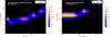 |
Fig. C.1 Likelihood maps in the parameter space [〈E〉, ψ] for a monoenergetic distribution (left) and a kappa distribution (right). The global maximum of the likelihood is marked by a green star. |
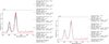 |
Fig. C.2 Fit of the observed spectrum in region 7 using the [〈E〉, ψ] parameters corresponding to the secondary likelihood maxima obtained for both the monoenergetic and kappa distribution cases. In both panels, the observed Juno/UVS spectrum for region 7 is shown in red, and the modeled spectra corresponding to the best-fit parameter pair [〈E〉, ψ] at the global maximum of the likelihood are shown in blue. The left panel corresponds to the monoenergetic distribution, and the right to the kappa distribution. Also shown are the modeled spectra associated with secondary local maxima in the likelihood maps. The local BIC is calculated by considering the local maximum of the likelihood in each case of the electron flux distribution considered in the model. |
However, considering the case of region 7, the results of our sensitivity study show that the effect on the intensities and the line ratio becomes significant for a surface albedo of about 10 to 20 % (see Fig. D.3). Therefore, in the absence of precise experimental constraints on this parameter, we conservatively adopted a zero value for the electron albedo in all simulations performed in this study.
Appendix D.3 Influence of the κ parameter on the ratio and brightness of the O I lines at 130.4 and 135.6 nm
To evaluate the influence of the κ parameter on the modeled auroral UV emissions at Ganymede, we conducted a sensitivity study focusing on region 10, where all electron distributions (monoenergetic, Maxwellian, and kappa) yield satisfactory fits to the observed spectrum of the auroral emissions. For this test, we adopted the best-fit parameters from the kappa-distribution case – namely, a mean energy of 〈E〉 = 300 eV and an energy flux ψ = 2 mW/m2 – and varied only the κ value in our electron transport model.
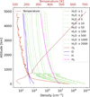 |
Fig. D.1 Atmospheric model initially presented in Fig. 2, including the different H2O profiles used in our sensitivity study. |
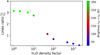 |
Fig. D.2 Evolution of the line ratio I(135.6 nm)/I(130.4 nm) as a function of the scaling factor applied solely to the vertical abundance profile of H2O. The total brightness of the modeled oxygen lines is also represented with color intensity. |
The kappa-type energy distribution used in our electron transport model is defined as
 (D.1)
(D.1)
where E is the electron energy, 〈E〉 is the mean energy of the distribution, κ is the suprathermal parameter controlling the high-energy tail, and Q0 is a free parameter. The characteristic energy E0, corresponding to the energy at which the distribution peaks, is related to the mean energy as
 (D.2)
(D.2)
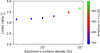 |
Fig. D.3 Evolution of the line ratio I(135.6 nm)/I(130.4 nm) as a function of the surface electron surface albedo applied in the TransPlanet model, considering the observation geometry of region 7. The surface albedo varies from 0% to 100%. The color intensity represents the evolution of the total brightness of the modeled oxygen spectral lines. |
This functional form allows for a continuous transition between Maxwellian-like distributions (high κ) and strongly non-thermal distributions (low κ), and is commonly used (e.g., Coumans et al. 2002; Salveter et al. 2022; Benmahi et al. 2024a,b) to describe suprathermal particle populations in space plasmas.
In this sensitivity study, we tested κ = 2.001, 2.1, 2.5, 3.0, 5.0, and 10.0, following the methodology of Benmahi et al. (2024b). These values cover the full range of kappa-distribution behavior used in our model: the lower limit (κ → 2) corresponds to a distribution with a strong high-energy tail, while the upper limit (κ ≫ 10) approximates a Maxwellian distribution.
Fig. D.3 shows that small variations in κ around 2.5 (e.g., between 2.1 and 3.0) have little effect on the line ratio I(135.6 nm)/I(130.4 nm), but significantly impact the total brightness of the oxygen emissions, as also shown by Benmahi et al. (2024b) for the jovian H2 emission case. This behavior reflects the role of κ in shaping the suprathermal tail of the electron energy distribution, which alters the balance between high-and low-energy electrons. These electrons interact differently with the atmospheric constituents, affecting the excitation rates of O(3S°) and O(5S°) and, hence, the resulting UV brightness.
This sensitivity study highlights the importance of κ in accurately retrieving electron energy fluxes from UV observations. Although beyond the scope of this study, tighter observational constraints on this parameter, particularly from in situ measurements by Juno/JADE and Juno/JEDI, would substantially refine the diagnostics presented in this study. Future data from the Particle Environment Package (PEP) instrument on board Juice could further improve our understanding of electron energy distributions in Ganymede’s auroral environment.
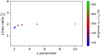 |
Fig. D.4 Line ratio I(135.6 nm)/I(130.4 nm) as a function of the κ parameter applied to the kappa distribution in the TransPlanet model for the fitting case of region 10. The color intensity represents the evolution of the total brightness of the modeled oxygen spectral lines. |
Appendix E Spectral fitting of auroral emissions across all analyzed regions
Appendix E, which presents additional figures and analysis supporting the interpretation of the retrieved electron properties, is available as supplementary material on Zenodo at: https://zenodo.org/records/17246180
All Tables
UV transitions of atomic oxygen from the excited states 3s 3Sº and 3s 5Sº to the ground state 2p4 3P.
All Figures
|
Fig. 1 Total brightness map of the atomic oxygen auroral emission lines around 130.4 and 135.6 nm observed during Juno’s PJ34 flyby of Ganymede. The yellow polygons (dashed lines) indicate the main auroral regions identified from the observations. The colored polygons (solid lines), magenta polygons numbered from 0 to 16, delineate the specific subregions investigated in this study. |
| In the text | |
|
Fig. 2 Average vertical profiles of the densities of the main chemical species of Ganymede’s atmosphere O2, H2O, O, H2, and H in the auroral regions, outlined by the yellow polygons in Fig. 1. These profiles were directly extracted from the atmospheric model of Vorburger et al. (2024). |
| In the text | |
|
Fig. 3 Top: UVS spectrum observed in region 7 (in gray). The blue, red, and green spectra are respectively the best fits obtained by considering a monoenergetic distribution, a Maxwellian distribution, and a kappa distribution. The estimated parameters [〈E〉, ψ] obtained from these fits with our model are shown in the legend. Bottom: residuals of the best fit for each type of electron energy flux distribution. For each distribution type, this residual is calculated by subtracting the best fit from the observed spectrum. |
| In the text | |
|
Fig. A.1 Three electron energy flux distributions with the same mean energy (100 eV) and energy flux (1 mW/m2): monoenergetic (blue), Maxwellian (red), and kappa with κ = 2.5 (green). |
| In the text | |
|
Fig. C.1 Likelihood maps in the parameter space [〈E〉, ψ] for a monoenergetic distribution (left) and a kappa distribution (right). The global maximum of the likelihood is marked by a green star. |
| In the text | |
|
Fig. C.2 Fit of the observed spectrum in region 7 using the [〈E〉, ψ] parameters corresponding to the secondary likelihood maxima obtained for both the monoenergetic and kappa distribution cases. In both panels, the observed Juno/UVS spectrum for region 7 is shown in red, and the modeled spectra corresponding to the best-fit parameter pair [〈E〉, ψ] at the global maximum of the likelihood are shown in blue. The left panel corresponds to the monoenergetic distribution, and the right to the kappa distribution. Also shown are the modeled spectra associated with secondary local maxima in the likelihood maps. The local BIC is calculated by considering the local maximum of the likelihood in each case of the electron flux distribution considered in the model. |
| In the text | |
|
Fig. D.1 Atmospheric model initially presented in Fig. 2, including the different H2O profiles used in our sensitivity study. |
| In the text | |
|
Fig. D.2 Evolution of the line ratio I(135.6 nm)/I(130.4 nm) as a function of the scaling factor applied solely to the vertical abundance profile of H2O. The total brightness of the modeled oxygen lines is also represented with color intensity. |
| In the text | |
|
Fig. D.3 Evolution of the line ratio I(135.6 nm)/I(130.4 nm) as a function of the surface electron surface albedo applied in the TransPlanet model, considering the observation geometry of region 7. The surface albedo varies from 0% to 100%. The color intensity represents the evolution of the total brightness of the modeled oxygen spectral lines. |
| In the text | |
|
Fig. D.4 Line ratio I(135.6 nm)/I(130.4 nm) as a function of the κ parameter applied to the kappa distribution in the TransPlanet model for the fitting case of region 10. The color intensity represents the evolution of the total brightness of the modeled oxygen spectral lines. |
| In the text | |
Current usage metrics show cumulative count of Article Views (full-text article views including HTML views, PDF and ePub downloads, according to the available data) and Abstracts Views on Vision4Press platform.
Data correspond to usage on the plateform after 2015. The current usage metrics is available 48-96 hours after online publication and is updated daily on week days.
Initial download of the metrics may take a while.