© The Authors 2025

1. Introduction

The Sun supports periodic and quasiperiodic oscillations over a wide range of spatial and temporal scales. In addition to the well-known five-minute acoustic modes of oscillation, it also exhibits quasi-toroidal modes in the inertial frequency range, with frequencies comparable to the solar rotation frequency. Solar equatorial Rossby modes were first detected by Löptien et al. (2018) and later confirmed by Liang et al. (2019) and Hanasoge & Mandal (2019). A rich spectrum of additional inertial modes, all retrograde in the Carrington frame, were identified in frequency-latitude space by Gizon et al. (2021). Of these, the mode with the largest amplitude is an m = 1 high-latitude mode with a north-south symmetric radial vorticity. The amplitude of this mode can be as high as 20 m/s at times. It is believed to be baroclinically unstable (Bekki et al. 2022) and saturates via a nonlinear interaction with the Sun’s latitudinal differential rotation (Bekki et al. 2024). The velocity features associated with this mode had been noticed at high latitudes by various authors; however, it was not then identified as a global mode of oscillation (Ulrich 1993, 2001; Hathaway et al. 2013; Bogart et al. 2015). For a recent review of solar inertial modes, we refer to Gizon et al. (2024).

The high-latitude modes were initially identified in long time series of near-surface flows in the longitudinal (u_ϕ) and colatitudinal (u_θ) directions. In particular, two modes with m = 1 and north-south symmetries were observed within 3 nHz of each other (Gizon et al. 2021). The mode with the significantly larger amplitude was antisymmetric in u_ϕ (symmetric in radial vorticity) and had a frequency ${\nu }_{\mathrm{HL}1}^{\mathrm{Carr}}=-86.3\pm 1.6$ nHz in the Carrington frame, with a linewidth of 7.8 ± 0.2 nHz and a mean amplitude of 9.8 m/s, over the period 2010−2020 (Gizon et al. 2021). The latitude at maximum amplitude was determined to be close to 67.5°. In a recent paper, Liang & Gizon (2025, hereafter LG25) measured the mode amplitude in direct Doppler data and found that the mode has remained visible above 60° latitude throughout the last five solar cycles, i.e., since 1967. LG25 report that the mode amplitude exhibits a negative correlation of −0.50 with the sunspot number and a strong negative correlation of −0.82 with the differential rotation rate near the mode’s critical latitude (the latitude at which its phase speed equals the rotational velocity).

In this Letter we show that the m = 1 high-latitude inertial mode is detectable in the line-of-sight (LOS) photospheric magnetic field, and we study the temporal evolution of its amplitude over a period of 17 years (2007 to 2024). In Sect. 2 we describe the datasets used. We detect and characterize the magnetic field oscillations in Sect. 3 and compare them to the velocity oscillations in Sect. 4. The results are discussed in Sect. 5.

2. Observational datasets

To investigate oscillations in the photospheric LOS magnetic field (B_los) in the inertial frequency range, we analyzed two long-term datasets. We used 720 s cadence LOS magnetograms taken by the Helioseismic and Magnetic Imager (HMI; Schou et al. 2012) on board the Solar Dynamics Observatory (SDO; Pesnell et al. 2012) over a time period of more than 14 years (2010−2024), as well as daily merged magnetograms from the Global Oscillation Network Group (GONG; Harvey et al. 1996) spanning 17 years (2007−2024). We compiled the datasets at a one-day cadence by computing daily averages when multiple images were available for a given day. The duty cycle of the daily averages is nearly 100% for both the HMI and GONG datasets. The original magnetograms have 4096 × 4096 pixels for HMI and 839 × 839 pixels for GONG. Unlike LG25, we did not use the Mount Wilson data because their signal-to-noise ratio is significantly lower.

The data reduction procedure, which was the same for both datasets, is as follows. Daily magnetograms were binned down to 256 × 256 pixels and remapped onto a uniform grid in Stonyhurst longitude (ϕ) and latitude (λ) with a grid spacing of 1° in both coordinates. We then computed the latitudinally symmetric component of the magnetic field as

$$\begin{array}{c}\hfill B_{\mathrm{los}}^{+}(\lambda ,\varphi ,t)=\frac{1}{2}[B_{\mathrm{los}}(\lambda ,\varphi ,t)+B_{\mathrm{los}}(-\lambda ,\varphi ,t)].\end{array}$$(1)

We also computed the antisymmetric component of B_los but found no significant signal in the neighborhood of the m = 1 mode frequency.

To further increase the signal-to-noise ratio, we considered averages of $B_{\mathrm{los}}^{+}$ in longitude at every time step:

$$\begin{array}{c}\hfill B_{\mathrm{avg}}^{+}(\lambda ,t)=\frac{1}{N_{\varphi }}{\displaystyle \sum _{|\varphi |\le {30}^{°}}}{B}_{\mathrm{los}}^{+}(\lambda ,\varphi ,t),\end{array}$$(2)

where N_ϕ = 61 is the number of longitude bins in the sum. To detect a perturbation in the magnetic field that may be associated with the high-latitude mode, we investigated the evolution of the magnetic field in the latitude range where the mode’s amplitude is most prominent (around or beyond 67.5°; see Gizon et al. 2021). We defined the latitudinal average of $B_{\mathrm{avg}}^{+}$ over the latitude band 65° ≤λ ≤ 70°:

$$\begin{array}{c}\hfill ⟨B_{\mathrm{avg}}^{+}⟩(t)=\frac{1}{N_{\lambda }}{\displaystyle \sum _{{65}^{°}\le \lambda \le {70}^{°}}}{B}_{\mathrm{avg}}^{+}(\lambda ,t),\end{array}$$(3)

where the N_λ = 6 is the number of latitude bins in the sum.

To compare the magnetic field signal with the mode characteristics derived from the reduced LOS Doppler velocity (V_los), we also computed the following quantities from the HMI and GONG Dopplergrams (see LG25 for details):

$$\begin{array}{cc}\hfill V_{\mathrm{zonal}}(\lambda ,t)& ={\displaystyle \frac{1}{{\sum }_{|\varphi |\le {30}^{°}}|sin\varphi |}\sum _{|\varphi |\le {30}^{°}}}(sin\varphi )V_{\mathrm{los}}(\lambda ,\varphi ,t),\hfill \end{array}$$(4)

$$\begin{array}{cc}\hfill V_{\mathrm{zonal}}^{-}(\lambda ,t)& =\frac{1}{2}[V_{\mathrm{zonal}}(\lambda ,t)-V_{\mathrm{zonal}}(-\lambda ,t)],\hfill \end{array}$$(5)

$$\begin{array}{cc}\hfill ⟨V_{\mathrm{zonal}}^{-}⟩(t)& =\frac{1}{N_{\lambda }}{\displaystyle \sum _{{65}^{°}\le \lambda \le {70}^{°}}}{V}_{\mathrm{zonal}}^{-}(\lambda ,t).\hfill \end{array}$$(6)

The zonal velocity, V_zonal, serves as a proxy for the longitudinal component of surface velocity (Ulrich 2001).

3. Detection of the m = 1 mode in magnetograms

Figure 1 shows super-synoptic maps of $B_{\mathrm{avg}}^{+}$ and $V_{\mathrm{zonal}}^{-}$ at high latitudes. An oscillating pattern is evident in both quantities with a temporal cadence of approximately 34 days. The oscillation is also clearly visible in the spatially averaged $⟨B_{\mathrm{avg}}^{+}⟩$ and $⟨V_{\mathrm{zonal}}^{-}⟩$ data in Fig. 2. We find an amplitude of up to 0.5 G for $⟨B_{\mathrm{avg}}^{+}⟩$, which is associated with the already known amplitude of 10−20 m/s for $⟨V_{\mathrm{zonal}}^{-}⟩$ in the latitude range 65° −70°. Since the magnetic field evolution appears to be tightly related to that of the m = 1 mode observed in the Doppler data (LG25), this strongly suggests the presence of the m = 1 mode in the magnetograms; however, this still needs to be verified through spectral analysis.

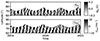Fig. 1. Super-synoptic maps in the Earth frame of $B_{\mathrm{avg}}^{+}$ and $V_{\mathrm{zonal}}^{-}$ at high latitudes, computed from HMI data for the period 2019−2020. The m = 1 mode manifests itself as a series of stripes in both observables. A 180-day running average was subtracted, and for clarity, the maps were smoothed using a Gaussian kernel with a width of two pixels in both latitude and time.

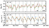Fig. 2. Oscillations of $⟨B_{\mathrm{avg}}^{+}⟩$ and $⟨V_{\mathrm{zonal}}^{-}⟩$ in the time series from HMI and GONG data in 2019. A 180-day average was removed, and for clarity, the maps were smoothed with a Gaussian kernel with σ = 1 day. Vertical lines are spaced at intervals of 34 days.

3.1. Power spectra

We examined $⟨B_{\mathrm{avg}}^{+}⟩$ in the frequency domain by performing a Fourier transform over the full time period available in each dataset. The power spectra were rescaled to account for the missing data in the time series. In the bottom row of Fig. 3, we show the power spectra of $⟨B_{\mathrm{avg}}^{+}⟩$ for the full HMI and GONG datasets. In both spectra, we find a great deal of excess power around 338 nHz, with a full width at half maximum of approximately 11 − 16 nHz (corresponding to an e-folding lifetime of ≈8 − 11 months). We recall that the frequency of the m = 1 mode was reported by Gizon et al. (2021) to be ${\nu }_{\mathrm{HL}1}^{\mathrm{Carr}}=-86.3$ nHz in the Carrington frame. In the Earth frame the mode frequency is

$$\begin{array}{c}\hfill {\nu }_{\mathrm{HL}1}^{\mathrm{synodic}}={\nu }_{\mathrm{HL}1}^{\mathrm{Carr}}+m({\mathrm{\Omega }}_{\mathrm{Carr}}-{\mathrm{\Omega }}_{\oplus })/2\pi =338\mathrm{nHz},\end{array}$$(7)

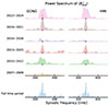Fig. 3. Power spectra of magnetic fluctuations $⟨B_{\mathrm{avg}}^{+}⟩$ over three-year intervals with a frequency resolution of 10.5 nHz for GONG (left) and HMI (right) data, stacked vertically and spanning from 2007 to 2024. The crosses mark the reference frequency of 338 nHz. The right-hand-side panel for 2007−2009 contains no data because the HMI dataset starts in 2010. The bottom spectra were computed using the entire available time span for each respective dataset.

where Ω_Carr/2π = 456 nHz is the Carrington rotation rate and Ω_⊕/2π = 31.7 nHz is the Earth’s mean orbital frequency around the Sun.

Figure 3 further shows changes in the power spectra of $⟨B_{\mathrm{avg}}^{+}⟩$ in three-year intervals for GONG and HMI data. It is evident that the signal is not uniformly strong over the entire time period, nor is it persistently present (i.e., significant); instead, it rises and wanes over cycle 24. The strongest and clearest signal is observed during the solar minimum interval of 2019−2021 with a peak amplitude of ≈4 × 10⁻⁴ G² nHz⁻¹, while no significant signal is observed in the period 2016−2018. We also find a clear signal from 2010−2015 with a peak amplitude of ≈3 × 10⁻⁴ G² nHz⁻¹. The GONG and HMI results are in very good agreement.

3.2. Latitudinal variation of the phase

We calculated the average phase of $B_{\mathrm{avg}}^{+}$ as a function of latitude using a temporal Fourier transform. Phase shifts relative to 67.5° latitude were extracted within a narrow band centered at 338 nHz (±10 nHz) and then averaged. The resulting phase, wrapped to the interval [−π, π], varies smoothly between 55° and 80° latitude (see Fig. A.1). The smooth variation suggests that the excess power at higher latitudes reflects a genuine mode signal rather than stochastic fluctuations. The phase becomes irregular at lower latitudes, where the mode power is not significant.

4. Comparison of B_los and V_los

We next compared the excess power around 338 nHz in the $⟨B_{\mathrm{avg}}^{+}⟩$ and $⟨V_{\mathrm{zonal}}^{-}⟩$ spectra. Following the procedure described by LG25 (their Sect. 5.2), we estimated the total power around the mode frequency by fitting a Lorentzian function. Figure 4 shows the temporal variations in the mode amplitude measured from overlapping 3-year time series, with central times spaced one year apart, starting in 2007 for $⟨B_{\mathrm{avg}}^{+}⟩$ and in 2003 for $⟨V_{\mathrm{zonal}}^{-}⟩$.

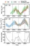Fig. 4. Top and middle panels: Temporal variations of the m = 1 mode amplitude extracted from Blos and Vlos data, respectively. The red, orange, green, and blue curves correspond to results from the HMI $⟨B_{\mathrm{avg}}^{+}⟩$, HMI $⟨V_{\mathrm{zonal}}^{-}⟩$, GONG $⟨B_{\mathrm{avg}}^{+}⟩$, and GONG $⟨V_{\mathrm{zonal}}^{-}⟩$ datasets, respectively. Shaded regions indicate the 68% confidence interval, estimated using 10 000 Monte Carlo simulations. Open circles denote instances where the excess power near the mode frequency falls below the 90% confidence level. We note that $⟨V_{\mathrm{zonal}}^{-}⟩$ was derived directly from the LOS Doppler velocity (Eqs. (4)–(6)); unlike LG25, we did not apply a multiplicative factor to scale the $⟨V_{\mathrm{zonal}}^{-}⟩$ amplitudes to match the horizontal velocities from the ring-diagram maps. Vertical lines denote key phases of the solar cycle, with solid lines representing solar minima and dashed lines indicating solar maxima. Bottom panel: Average sunspot number (source: WDC-SILSO, Royal Observatory of Belgium, Brussels, https://doi.org/10.24414/qnza-ac80).

We find very good agreement between the GONG and HMI results for each respective quantity. The mode amplitudes seen in $⟨B_{\mathrm{avg}}^{+}⟩$ and $⟨V_{\mathrm{zonal}}^{-}⟩$ are positively correlated, but there is a time lag between the magnetic field and velocity perturbations. The maximum amplitude in $⟨B_{\mathrm{avg}}^{+}⟩$ is about 0.2 G in 2012 and again around 2020−2023. Both $⟨B_{\mathrm{avg}}^{+}⟩$ and $⟨V_{\mathrm{zonal}}^{-}⟩$ are moderately anticorrelated with the sunspot number, but the mode amplitudes measured in $⟨B_{\mathrm{avg}}^{+}⟩$ appear to reach a maximum during rising phases of the sunspot cycle.

Figure 5 shows frequency-filtered images of the LOS Doppler velocity, V_los, and the LOS magnetic field, B_los, derived from HMI observations. A bandpass filter centered at ${\nu }_{\mathrm{HL}1}^{\mathrm{synodic}}=338$ nHz with a full width of 30 nHz was applied to retain the m = 1 mode. We emphasize that no spatial Fourier transform was applied. For V_los, the structure of the mode is clearly visible at high latitudes, while little to no signal is present at lower latitudes. The B_los data also show the mode at high latitudes, but the lower latitudes display a plethora of signals associated with residual magnetic activity and not related to the mode. The bottom panels of Fig. 5 show synoptic maps of V_los and B_los, constructed by stacking the central meridian from bandpass-filtered images over time. The m = 1 mode appears as inclined stripes in time-latitude space. A similar pattern was already visible in the synoptic maps of Fig. 1 in the absence of a frequency filter.

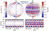Fig. 5. Bandpass-filtered images of the LOS Doppler velocity, Vlos, and LOS magnetic field, Blos, derived from HMI data. Top left: Filtered Vlos image from 14 June 2020. Bottom left: Central-meridian Vlos values stacked over time and plotted as a function of time and latitude. Right panels: Corresponding Blos data, with low-latitude regions (< 45°) shaded out. The filtering was performed using a bandpass filter centered at ${\nu }_{\mathrm{HL}1}^{\mathrm{synodic}}=338$ nHz with a full width of 30 nHz, applied over the entire available HMI time period, i.e., from 2010 to 2024. For clarity, the images were smoothed with a Gaussian kernel with a width of 2 pixel – in longitude and latitude (top panels) and in time and latitude (bottom panels). A movie is available as online supplementary material.

5. Discussion

We identified a coherent magnetic field oscillation at a frequency of 338 nHz (with a frequency resolution of 10.5 nHz) and a peak amplitude of about 0.2 G in B_los. This oscillation is associated with the high-latitude m = 1 global inertial mode previously characterized in the velocity data. The B_los perturbations are predominantly symmetric across the equator, in contrast to the V_los perturbations, which are primarily north-south antisymmetric. The magnetic field oscillations are most clearly observed at latitudes above 60° during the recent solar minimum (2018−2022). The mode amplitude in $⟨B_{\mathrm{avg}}^{+}⟩$ peaks around 2012, during the rising phase of cycle 24, and again in 2020−2023, the rising phase of cycle 25. A time lag of approximately two years is observed between the trends in the magnetic and velocity perturbations.

As outlined in a simple model in Appendix B, the amplitude of the magnetic oscillation during solar cycle minimum may be understood via the linearized induction equation, Eq. (B.3), whereby the radial magnetic field is advected by the hydrodynamic high-latitude mode. This simple model approximately reproduces the symmetric pattern at high latitudes with a maximum amplitude of ≈0.2 G. The calculation assumes a dipolar background field magnetic field during solar minimum (Fig. B.1). It would be interesting to repeat these calculations over different phases of the solar cycle using, for example, a background magnetic field from a dynamo model.

Data availability

Movie associated with Fig. 5 is available at https://www.aanda.org

Acknowledgments

The observations were analyzed by SGH and Z-CL. The analytical model was derived by LG and Z-CL. This research was funded in whole, or in part, by the Austrian Science Fund (FWF) [10.55776/J4560]. For the purpose of open access, the author has applied a CC BY public copyright licence to any Author Accepted Manuscript version arising from this submission. SGH acknowledges funding from the Research Council of Finland (RCF) Academy Fellowship [370747: RIB-Wind]. We thank B. Proxauf and S. Good for valuable discussions. This work utilizes GONG data from NSO, which is operated by AURA under a cooperative agreement with NSF and with additional financial support from NOAA, NASA, and USAF. The HMI data used are courtesy of NASA/SDO and the HMI science team.

References

Appendix A: Phase of magnetic oscillations as a function of latitude

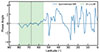Fig. A.1. Latitudinal dependence of the phase of $B_{\mathrm{avg}}^{+}$ relative to latitude 67.5°, measured during solar minimum (2018−2021) and at the frequency of the m = 1 high-latitude mode. The green shaded area highlights the latitude range where the phase varies smoothly. This coincides with the latitude range where the mode has the largest amplitudes in the power spectrum.

Appendix B: Simplified model for magnetic field perturbations during cycle minimum

Let us consider the induction equation in an inertial frame,

$$\begin{array}{c}\hfill {\partial }_t\mathbf{B}=\eta \mathrm{\Delta }\mathbf{B}+\mathrm{\nabla }\times (\mathbf{v}\times \mathbf{B}).\end{array}$$(B.1)

Assuming background values of the magnetic field (B₀) and of the axisymmetric flow (v₀) during solar minimum, we wished to compute the perturbations to the magnetic field at the surface (B′) caused by the fluctuating flow (v′) associated with a mode of oscillation. In the near-surface layers, the velocity field of a quasi-toroidal mode of oscillation is approximately horizontal and divergence-free,

$$\begin{array}{c}\hfill \mathbf{v}\prime =\mathfrak{R}\{\mathbf{u}\prime (\theta )e^{\mathrm{i}m\varphi -\mathrm{i}\omega t}\},\mathrm{\nabla }·\mathbf{v}\prime =0.\end{array}$$(B.2)

The magnetic field was assumed to be purely radial at the surface. We linearized the induction equation to obtain an equation for the magnetic field perturbation (B′):

$$\begin{array}{c}\hfill {\partial }_t\mathbf{B}\prime -\mathrm{\nabla }\times ({\mathbf{v}}_0\times \mathbf{B}\prime )-\eta \mathrm{\Delta }\mathbf{B}\prime =\mathrm{\nabla }\times (\mathbf{v}\prime \times {\mathbf{B}}_0).\end{array}$$(B.3)

Taking the radial component of this equation, we have

$$\begin{array}{c}\hfill {\partial }_t{B}_r\prime +\mathrm{\nabla }·({\mathbf{v}}_0{B}_r\prime )-\eta \mathrm{\Delta }{B}_r\prime =-(\mathbf{v}\prime ·\mathrm{\nabla })B_{0r},\end{array}$$(B.4)

where we used ∇ ⋅ B₀ = 0 and ∇ ⋅ v′ = 0.

During solar minimum, the background field at the surface is approximately radial at the surface and independent of longitude, that is, ${\mathbf{B}}_0=B_{0r}(\theta )\widehat{\mathbf{r}}$. As shown in Fig. B.1, a reasonable model for the field is B_0r ≈ b₀(cos θ)ⁿ with b₀ = 10 G and n = 7. The background flow consists of rotation and the meridional flow, that is, ${\mathbf{v}}_0=Rsin\theta \mathrm{\Omega }(\theta )\widehat{\mathit{\varphi }}+v_{\mathrm{MC}}(\theta )\widehat{\mathit{\theta }}$. We used the surface angular velocity profile Ω(θ) from Snodgrass (1984) and the meridional flow profile v_MC(θ) = − 15 sin(2θ) sin θ m/s.

Next, we plugged perturbations to the magnetic field of the form B_r′=ℜ{b′(θ)e^{imϕ − iωt}} into Eq. (B.4) to obtain

$$\begin{array}{c}\hfill -\mathrm{i}\omega b\prime +\mathrm{i}m\mathrm{\Omega }b\prime +\frac{1}{Rsin\theta }\frac{d}{d\theta }(sin\theta (v_{\mathrm{MC}}b\prime -\frac{\eta }{R}\frac{db\prime }{d\theta }))+\frac{\eta m^{2}b\prime }{{(Rsin\theta )}^2}=-\frac{u{\prime }_{\theta }(\theta )}{R}\frac{d{B}_{0r}}{d\theta }.\end{array}$$(B.5)

We adopted a surface diffusivity of η = 250 km²/s, consistent with the supergranulation. The right-hand side (RHS) of the equation depends on the co-latitudinal component of the m = 1 high-latitude (HL1) mode velocity, u′_θ(θ), which we extracted from HMI ring-diagram flow maps along the central meridian at the HL1 mode frequency. As a sanity check, we separately computed the left-hand side (LHS) of the equation using the observed b′ as input, and the RHS of the equation using the observed u′_θ. At latitudes above 60° (i.e., above the critical latitude of the HL1 mode), we find that the two sides of the equation have comparable amplitudes. We also find that the diffusion and meridional flow terms on the LHS of Eq. (B.5) are negligible. This implies that a rough estimate for b′ is

$$\begin{array}{c}\hfill b\prime (\theta )\approx \frac{\mathrm{i}u{\prime }_{\theta }}{R(m\mathrm{\Omega }-\omega )}\frac{d{B}_{0r}}{d\theta }\mathrm{for}\theta \ll {\theta }_c,\end{array}$$(B.6)

where θ_c = 32° is the critical colatitude given by Ω(θ_c) = ω/m. Figure B.2 compares the LOS projection of the fluctuating magnetic field derived from Eq. (B.6) to the observed $B_{\mathrm{avg}}^{+}$ during cycle minimum (also see Fig. 1). Although the approximate model does not perfectly reproduce the observations (especially the phase), it provides the correct order-of-magnitude estimate for the observed $B_{\mathrm{avg}}^{+}$. We therefore conclude that the observed magnetic field perturbations at the surface are largely caused by the passive advection of the radial field (B_r′) by the HL1 mode (velocity v′_θ).

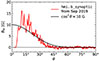Fig. B.1. Background radial magnetic field during solar minimum estimated from the data series hmi.b_synoptic (Liu et al. 2017). The synoptic maps for the radial component of the magnetic field were stacked in time and then Gaussian-smoothed with a full width of 27 days. The red curve shows the data in the northern hemisphere on 15 September 2019, when the Sun was quiet and its north pole was tilted toward the Earth. The black curve shows the approximation B0r(θ) = 10 × (cos θ)7 G, which we use in Eqs. (B.5) and (B.6).

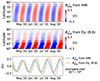Fig. B.2. Top: Observed $B_{\mathrm{avg}}^{+}$ using HMI magnetograms at the HL1 mode frequency during solar minimum. Middle: Estimate of $B_{\mathrm{avg}}^{+}$ above the critical latitude using the approximation given by Eq. (B.6). Bottom: Comparison of observed and modeled values, after averaging over the latitudinal band 65° −70°.

All Figures

Fig. 1. Super-synoptic maps in the Earth frame of $B_{\mathrm{avg}}^{+}$ and $V_{\mathrm{zonal}}^{-}$ at high latitudes, computed from HMI data for the period 2019−2020. The m = 1 mode manifests itself as a series of stripes in both observables. A 180-day running average was subtracted, and for clarity, the maps were smoothed using a Gaussian kernel with a width of two pixels in both latitude and time.

In the text

	Fig. 2. Oscillations of $⟨B_{\mathrm{avg}}^{+}⟩$ and $⟨V_{\mathrm{zonal}}^{-}⟩$ in the time series from HMI and GONG data in 2019. A 180-day average was removed, and for clarity, the maps were smoothed with a Gaussian kernel with σ = 1 day. Vertical lines are spaced at intervals of 34 days.
In the text

Fig. 3. Power spectra of magnetic fluctuations $⟨B_{\mathrm{avg}}^{+}⟩$ over three-year intervals with a frequency resolution of 10.5 nHz for GONG (left) and HMI (right) data, stacked vertically and spanning from 2007 to 2024. The crosses mark the reference frequency of 338 nHz. The right-hand-side panel for 2007−2009 contains no data because the HMI dataset starts in 2010. The bottom spectra were computed using the entire available time span for each respective dataset.

In the text

Fig. 4. Top and middle panels: Temporal variations of the m = 1 mode amplitude extracted from Blos and Vlos data, respectively. The red, orange, green, and blue curves correspond to results from the HMI $⟨B_{\mathrm{avg}}^{+}⟩$, HMI $⟨V_{\mathrm{zonal}}^{-}⟩$, GONG $⟨B_{\mathrm{avg}}^{+}⟩$, and GONG $⟨V_{\mathrm{zonal}}^{-}⟩$ datasets, respectively. Shaded regions indicate the 68% confidence interval, estimated using 10 000 Monte Carlo simulations. Open circles denote instances where the excess power near the mode frequency falls below the 90% confidence level. We note that $⟨V_{\mathrm{zonal}}^{-}⟩$ was derived directly from the LOS Doppler velocity (Eqs. (4)–(6)); unlike LG25, we did not apply a multiplicative factor to scale the $⟨V_{\mathrm{zonal}}^{-}⟩$ amplitudes to match the horizontal velocities from the ring-diagram maps. Vertical lines denote key phases of the solar cycle, with solid lines representing solar minima and dashed lines indicating solar maxima. Bottom panel: Average sunspot number (source: WDC-SILSO, Royal Observatory of Belgium, Brussels, https://doi.org/10.24414/qnza-ac80).

In the text

Fig. 5. Bandpass-filtered images of the LOS Doppler velocity, Vlos, and LOS magnetic field, Blos, derived from HMI data. Top left: Filtered Vlos image from 14 June 2020. Bottom left: Central-meridian Vlos values stacked over time and plotted as a function of time and latitude. Right panels: Corresponding Blos data, with low-latitude regions (< 45°) shaded out. The filtering was performed using a bandpass filter centered at ${\nu }_{\mathrm{HL}1}^{\mathrm{synodic}}=338$ nHz with a full width of 30 nHz, applied over the entire available HMI time period, i.e., from 2010 to 2024. For clarity, the images were smoothed with a Gaussian kernel with a width of 2 pixel – in longitude and latitude (top panels) and in time and latitude (bottom panels). A movie is available as online supplementary material.

In the text

	Fig. A.1. Latitudinal dependence of the phase of $B_{\mathrm{avg}}^{+}$ relative to latitude 67.5°, measured during solar minimum (2018−2021) and at the frequency of the m = 1 high-latitude mode. The green shaded area highlights the latitude range where the phase varies smoothly. This coincides with the latitude range where the mode has the largest amplitudes in the power spectrum.
In the text

Fig. B.1. Background radial magnetic field during solar minimum estimated from the data series hmi.b_synoptic (Liu et al. 2017). The synoptic maps for the radial component of the magnetic field were stacked in time and then Gaussian-smoothed with a full width of 27 days. The red curve shows the data in the northern hemisphere on 15 September 2019, when the Sun was quiet and its north pole was tilted toward the Earth. The black curve shows the approximation B0r(θ) = 10 × (cos θ)7 G, which we use in Eqs. (B.5) and (B.6).

In the text

	Fig. B.2. Top: Observed $B_{\mathrm{avg}}^{+}$ using HMI magnetograms at the HL1 mode frequency during solar minimum. Middle: Estimate of $B_{\mathrm{avg}}^{+}$ above the critical latitude using the approximation given by Eq. (B.6). Bottom: Comparison of observed and modeled values, after averaging over the latitudinal band 65° −70°.
In the text

References

- Bekki, Y., Cameron, R. H., & Gizon, L. 2022, A&A, 662, A16 [NASA ADS] [CrossRef] [EDP Sciences] [Google Scholar]
- Bekki, Y., Cameron, R. H., & Gizon, L. 2024, Sci. Adv., 10, eadk5643 [NASA ADS] [CrossRef] [Google Scholar]
- Bogart, R. S., Baldner, C. S., & Basu, S. 2015, ApJ, 807, 125 [NASA ADS] [CrossRef] [Google Scholar]
- Gizon, L., Cameron, R. H., Bekki, Y., et al. 2021, A&A, 652, L6 [NASA ADS] [CrossRef] [EDP Sciences] [Google Scholar]
- Gizon, L., Bekki, Y., Birch, A. C., et al. 2024, IAU Symp., 365, 207 [Google Scholar]
- Hanasoge, S., & Mandal, K. 2019, ApJ, 871, L32 [Google Scholar]
- Harvey, J. W., Hill, F., Hubbard, R. P., et al. 1996, Science, 272, 1284 [Google Scholar]
- Hathaway, D. H., Upton, L., & Colegrove, O. 2013, Science, 342, 1217 [NASA ADS] [CrossRef] [Google Scholar]
- Liang, Z.-C., & Gizon, L. 2025, A&A, 695, A67 [NASA ADS] [CrossRef] [EDP Sciences] [Google Scholar]
- Liang, Z.-C., Gizon, L., Birch, A. C., & Duvall, T. L. 2019, A&A, 626, A3 [NASA ADS] [CrossRef] [EDP Sciences] [Google Scholar]
- Liu, Y., Hoeksema, J. T., Sun, X., & Hayashi, K. 2017, Sol. Phys., 292, 29 [NASA ADS] [CrossRef] [Google Scholar]
- Löptien, B., Gizon, L., Birch, A. C., et al. 2018, Nat. Astron., 2, 568 [Google Scholar]
- Pesnell, W. D., Thompson, B. J., & Chamberlin, P. C. 2012, Sol. Phys., 275, 3 [Google Scholar]
- Schou, J., Scherrer, P. H., Bush, R. I., et al. 2012, Sol. Phys., 275, 229 [Google Scholar]
- Snodgrass, H. B. 1984, Sol. Phys., 94, 13 [NASA ADS] [CrossRef] [Google Scholar]
- Ulrich, R. K. 1993, ASP Conf. Ser., 40, 25 [NASA ADS] [Google Scholar]
- Ulrich, R. K. 2001, ApJ, 560, 466 [CrossRef] [Google Scholar]