| Issue |
A&A
Volume 704, December 2025
|
|
|---|---|---|
| Article Number | A258 | |
| Number of page(s) | 22 | |
| Section | Galactic structure, stellar clusters and populations | |
| DOI | https://doi.org/10.1051/0004-6361/202553814 | |
| Published online | 23 December 2025 | |
Chronology of our Galaxy from Gaia colour–magnitude diagram fitting (ChronoGal)
II. Unveiling the formation and evolution of the kinematically selected thick and thin discs
1
Departamento de Astrofísica, Universidad de La Laguna,
38205
La Laguna, Tenerife,
Spain
2
Instituto de Astrofísica de Canarias,
38200
La Laguna, Tenerife,
Spain
3
Dpto. de Física Teórica y del Cosmos, University of Granada,
Facultad de Ciencias (Edificio Mecenas),
18071
Granada,
Spain
4
Instituto Carlos I de Física Teórica y Computacional,
Universidad de Granada,
18071
Granada,
Spain
5
INAF – Astronomical Observatory of Abruzzo, via M. Maggini,
sn,
64100
Teramo,
Italy
6
INFN, Sezione di Pisa,
Largo Pontecorvo 3,
56127
Pisa,
Italy
7
Kapteyn Astronomical Institute, University of Groningen,
Landleven 12,
9747 AD Groningen,
The Netherlands
8
Leibniz-Institut fur Astrophysik Potsdam (AIP),
An der Sternwarte 16,
14482
Potsdam,
Germany
9
Université Côte d’Azur, Observatoire de la Côte d’Azur, CNRS,
Laboratoire Lagrange,
Nice,
France
★ Corresponding author: This email address is being protected from spambots. You need JavaScript enabled to view it.
Received:
20
January
2025
Accepted:
13
August
2025
Abstract
Context. Investigation of the formation, origin, and evolution of the dichotomy of the Milky Way’s thin and thick disc components has been a focal point of research since it is key to understanding the formation of our Galaxy. One difficulty in this pursuit is that the populations defined based on their morphology or kinematics show a mix of chemically distinct populations. Age is then a key parameter to understand the disc evolution.
Aims. We aim to derive age and metallicity distributions of the kinematic thick and thin discs in order to reveal details of the duration, intensity, and relation between the star formation episodes that led to the current kinematic thick-thin disc configuration.
Methods. We applied the CMDft.Gaia pipeline based on a colour-magnitude diagram fitting technique to derive the dynamically evolved star formation history (deSFH) of the kinematically selected thin and thick discs. The analysis is based on Gaia DR3 data within a cylindrical volume centred on the Sun with a radius of 250 pc and a height of 1 kpc.
Results. Our analysis shows that the kinematically selected thick disc is predominantly older than 10 Gyr and underwent a rapid metallicity enrichment through three main episodes. The first occurred over 12 Gyr ago, peaking at [Z/H] ∼−0.5 dex; the second was around 11 Gyr ago and caused a rapid increase in metallicity up to [Z/H]=0.0 and a broad spread in [α/Fe] from ∼ 0.3 to solar values; and the third, just over 10 Gyr ago, reached super-solar metallicities. In contrast, the kinematic thin disc stars began forming about 10 Gyr ago, coinciding with the thick disc’s star formation end, and is characterised by a super-solar metallicity and low [α/Fe]. The transition between the kinematic thick and thin discs aligns with the Milky Way’s last major merger: the accretion of Gaia-Sausage-Enceladus (GSE). We also identify a small population of kinematically selected thin disc stars with high and intermediate-[α/Fe] abundances, slightly older than 10 billion years, indicating a kinematic transition from thick to thin disc during the Milky Way’s high and intermediate- [α/Fe] phase. The kinematic thin disc’s age-metallicity relation reveals overlapping star formation episodes with distinct metallicities, suggesting radial mixing in the solar neighbourhood, with the greatest spread around 6 Gyr ago. Additionally, we detect an isolated thick disc star formation event 6 Gyr ago at solar metallicity, and it coincides with the estimated first pericentre of the Sagittarius satellite galaxy.
Key words: Galaxy: disk / Galaxy: evolution / Galaxy: formation / Galaxy: kinematics and dynamics / Galaxy: stellar content
© The Authors 2025
 Open Access article, published by EDP Sciences, under the terms of the Creative Commons Attribution License (https://creativecommons.org/licenses/by/4.0), which permits unrestricted use, distribution, and reproduction in any medium, provided the original work is properly cited.
This article is published in open access under the Subscribe to Open model. This email address is being protected from spambots. You need JavaScript enabled to view it. to support open access publication.
1 Introduction
Understanding galaxies is crucial for grasping the fundamental principles that govern the Universe. As the primary building blocks of the cosmos, their formation and evolution are intimately connected to the factors that drive cosmic development, such as the mechanisms that initiate and sustain star formation. Thus, observing and characterising galaxies provides valuable data that are critical for testing and refining cosmological models.
The processes that either trigger or quench star formation in galaxies leave distinctive imprints on the chemical and dynamical properties of their stars (Freeman & Bland-Hawthorn 2002). One of the morphological characteristics observed in disc galaxies, including in the Milky Way, is the presence of both a thick and a thin stellar disc (Tsikoudi 1979; Gilmore & Reid 1983; Morrison et al. 1994; Dalcanton & Bernstein 2002; Yoachim & Dalcanton 2008; Comerón et al. 2011). For some time, analysis of their properties indicated that thick discs should be among the oldest stellar components of galaxies (Seth et al. 2005; Elmegreen & Elmegreen 2006; Yoachim & Dalcanton 2006; Comerón et al. 2014; Haywood et al. 2013; Bovy et al. 2016). However, more recent studies combining observations with cosmological simulations consider that star formation in some thick discs could be sustained during longer times (Pinna et al. 2024).
The study of thick and thin discs and their relation provides key insights into the conditions and processes prevailing during the early stages of galaxy formation. Notably, our Galaxy offers a unique opportunity to study the formation and evolution of the disc in far greater detail than is possible in any other galaxy. In observed edge-on disc galaxies, a thin and a thick disc component are usually required to fit the stellar light (Yoachim & Dalcanton 2006), and the same is true for the Milky Way, where the number density distribution of stars in the solar neighbourhood is well fit by two exponential discs (thin and thick) with scale heights of 300 and 900 pc (Jurić et al. 2008, although see more recent measurements in Khanna et al. 2025). This constitutes a ‘geometric‘definition of the thin and thick discs, which is in fact the only currently possible definition in the case of distant galaxies. In the Milky Way, it has been found that thick disc stars tend to move in more eccentric and hotter orbits than thin disc stars: they lag behind the local standard of rest by about 50 km s−1 in the solar neighbourhood (Soubiran et al. 2003; Bensby et al. 2003). Thus, a ‘kinematic‘definition of the two components is sometimes used. Finally, the chemical composition of thick disc stars is overall more metal-poor and has a higher content of α elements with respect to iron compared to thin disc stars (Fuhrmann 1998; Bensby et al. 2003; Adibekyan et al. 2012; Hayden et al. 2015; Queiroz et al. 2020; Fuhrmann & Chini 2021), leading to a ‘chemical’ definition of the thin and thick disc populations that is possibly the most commonly used today. It is important to bear in mind that geometrically, kinematically, and chemically defined thin and thick discs do not result in identical populations (Kawata & Chiappini 2016). In fact, studies exploring stellar populations defined based on their chemical composition show the overlapping of these populations in kinematic and geometric space (Anders et al. 2018). Therefore, it is necessary to specify how a disc population has been defined in any detailed discussion of their properties and possible origin.
Even so, the overall hotter kinematics and larger α-element content of Milky Way thick disc stars in any of these definitions are usually interpreted as being indicative of having formed early in the history of the galaxy, during a time of high dynamical activity (based on predictions of cosmological simulations; e.g. Brook et al. 2004), and in an environment enriched by Type II supernovae over a period of rapid star formation before Type Ia supernovae became significant contributors (based on predictions of chemical evolution models Matteucci & Greggio 1986; Pagel & Tautvaišiené 1995; Chiappini et al. 1997; Kobayashi et al. 2011; Snaith et al. 2014; Grisoni et al. 2017; Grand et al. 2018; Spitoni et al. 2021). Stellar age determinations have broadly confirmed this scenario (Bensby et al. 2003; Haywood et al. 2013; Feuillet et al. 2018; Gallart et al. 2019; Miglio et al. 2021; Sahlholdt et al. 2022; Xiang & Rix 2022; Queiroz et al. 2023; Gallart et al. 2024; Pinsonneault et al. 2025), showing that high- α stars are typically older than 9−10 Gyr, while low- α stars are younger overall and cover a broader range of ages. However, there is no total consensus on the idea that the thick disc is a separate, discrete component of the Milky Way, and some authors have advocated for continuity in the properties of thick and thin discs and thus in their formation processes (Bovy et al. 2012; Recio-Blanco et al. 2014; Sharma et al. 2021; Prantzos et al. 2023).
Since the advent of all sky surveys such as SDSS/SEGUE (Yanny et al. 2009), SDSS/APOGEE (Majewski et al. 2017), RAVE (Steinmetz et al. 2020), GALAH (Buder et al. 2021), Gaia-ESO (Randich et al. 2022), and Gaia (Gaia Collaboration 2016), the characterisation of Milky Way stellar populations has significantly improved, but the evidence provided is still insufficient to fully answer fundamental open questions. For instance, there is a great uncertainty about the exact timing and duration of star formation in each disc, how the observed properties have varied over time, and what was the role of mergers, gas accretion, and secular evolution to shape the two discs.
To understand the true sequence of events that led to the present-day configuration of the Milky Way, precise age determinations for large and unbiased samples of stars are necessary. Until recently, precise stellar ages were achieved using techniques such as isochrone fitting (Sahlholdt et al. 2022; Xiang & Rix 2022, Queiroz et al. 2023) or asteroseismology (Chaplin & Miglio 2013; Lebreton & Goupil 2014; Silva Aguirre et al. 2015; Serenelli et al. 2017; Mackereth et al. 2019; Miglio et al. 2021), but they were available for relatively small samples, usually tailored to spectroscopic surveys affected by restrictive selection functions, thus limiting the information that their analysis could provide. A promising pathway to overcome these limitations has been opened with the ChronoGal project (Gallart et al. 2024), which uses the colour-magnitude diagram (CMD) fitting technique (Tolstoy & Saha 1996; Gallart et al. 1996; Hernandez et al. 1999; Dolphin 2002; Aparicio & Gallart 2004; Cignoni & Tosi 2010) on Gaia data to obtain precise age and metallicity distributions of vast samples of Milky Way stellar populations. While successful in studies of Local Group dwarf galaxies (e.g. Gallart et al. 1999a; Hernandez et al. 2000a; Noël et al. 2007; Bernard et al. 2007; Hidalgo et al. 2009; Monelli et al. 2010; Weisz et al. 2012; Hidalgo et al. 2013; Cignoni et al. 2013; Weisz et al. 2014; Cole et al. 2014; Gallart et al. 2015; Skillman et al. 2017; McQuinn et al. 2024), this technique has not been widely used for the Milky Way1 due to a lack of precise distance measurements for significant samples of stars until the advent of the Gaia mission, which is now providing unprecedented precision in parallax and photometry for stars within a large Milky Way volume.
Since the pioneering works by Gallart et al. (2019) and Ruiz-Lara et al. (2020), a more refined and optimised suite of codes, CMDft.Gaia (Gallart et al. 2024), has been developed to deliver high age precision (around 5%) and accuracy (∼ 6%)2 for complete samples of stellar populations in the Milky Way, providing a crucial missing piece of information for reconstructing our Galaxy’s history. The Milky Way stellar samples analysed in this way contain a mix of populations that formed locally and migrated from their birth site via dynamical processes. For this reason, we refer to the star formation histories (SFHs) derived by ChronoGal as ‘dynamically evolved star formation histories’ (deSFHs), and they provide the amount of mass per unit time and metallicity that has been transformed into stars somewhere in the galaxy to account for the stars that currently populate the studied volume. As part of the analysis performed by CMDft.Gaia, the distribution of ages and metallicities of the stars currently present in the analysed sample is also obtained. A detailed explanation of CMDft.Gaia is presented in the first paper of this series (Gallart et al. 2024 – Paper I).
Paper I also presents and discusses the most detailed deSFH ever inferred for the solar neighbourhood, within a spherical volume of 100 pc from the Sun, using the exquisite CMD of the Gaia Catalogue of Nearby Stars (Gaia Collaboration 2021). In this present paper, the second in the series, we aim to extend this analysis by deriving the deSFHs for the thin and thick discs selected kinematically over a broader volume in order to shed new light on their origins and evolutionary pathways.
This paper is organised as follows: in Section 2 we detail the data we analysed, the kinematic selection criteria applied, and the methodology used to derive the deSFHs. Section 3 presents the resulting deSFHs, with a detailed evaluation of the age-metallicity distributions (AMDs) of the thin and thick discs and their correlation with chemical abundance trends derived from spectroscopic databases. Section 4 discusses the implications of these findings for our understanding of the formation of the thick and thin discs. Finally, in Section 5 we summarise the main conclusions of the study.
2 Data and methodology
2.1 Volume definition and quality cuts
We selected stars within a cylindrical volume with a radius of 250 pc and a total height of 1 kpc centred on the Sun. This very local volume was chosen to simultaneously ensure (i) a high precision in astrometric parameters and photometry, enabling us to derive accurate CMDs in the absolute magnitude plane, and (ii) the required number of stars (increased by two orders of magnitude compared to the sample analysed in Paper I) in order to separate our final sample into the three main stellar populations it contains (thin disc, thick disc, and halo) and accurately infer the deSFH for each disc component separately.
An additional reason for this selection is that a nearby sample minimises the effects of extinction across the Galactic plane. However, extinction is not entirely negligible even within 250 pc of the Sun. To address this, we correct the Gaia DR3 photometry using state-of-the-art extinction maps. Specifically, we apply both the map by Lallement et al. (2022) and Vergely et al. (2022) (L22 from now on), and the map by Green et al. (2019) (G19). For the L22 map, to enhance efficiency in determining the extinction for each star, we pre-compute mean extinction values within healpixels across Galactic latitude and longitude at various distances from the cubes provided at three different resolutions by the authors. For the G19 map, we use the dustmaps-bayestar3 Python package, and adjust some values where extinction was reported as zero, as these cases were likely underestimated (G. Green, private communication). The results obtained with each of the extinction maps are similar and consistent. Thus, from here we focus on the results obtained when applying L22 extinction corrections as this map provides extinction measurements for all the sky while G19 only covers the North Hemisphere.
To convert the extinction in E(B-V) to AG, we follow the prescription suggested by the Gaia Collaboration, as detailed in Fitzpatrick et al. (2019). Consistent with Gallart et al. (2019) and Ruiz-Lara et al. (2020), we restrict our selection to stars with relatively low extinction, specifically AG<0.5.
We also cleaned our sample from stars that have unreliable photometry by selecting those verifying the following condition4:
 and
and

Finally, we computed the distances as the inverse of the parallax, selecting only stars with a relative parallax uncertainty of less than 20%. This criterion ensures that the inverse parallax provides a reliable value of the distance. We account for individual zero-point offsets as estimated by Lindegren et al. (2021) and include a systematic uncertainty of 0.015 mas in the zero-point (Lindegren et al. 2021).
2.2 Kinematic selection
We used Gaia DR3 parallaxes, proper motions and line-of-sight velocities to calculate the Cartesian velocity components with respect to the Galactic Reference Frame, U, V, W (considering the sun position with respect to the Galactic centre at 8.178 kpc (GRAVITY Collaboration 2019) and motion with respect to the local standard of Rest (U⊙, V⊙, W⊙)=(11.1, 12.24, 7.25) km s−1 (Schönrich et al. 2010), and positive values in the direction towards the Galactic centre, the sense of rotation of the Sun around the Galactic centre and the direction towards the north Galactic pole). Based on these velocities, it is possible to explore the kinematic stellar populations present in our sample. To this end, we have adopted the procedure by Bensby et al. (2003) to calculate probability distribution functions for each star to be a member of the thin, the thick disc or the halo by taking into account their velocity and their position within the Galaxy. Notice that this is not identical to the chemical thick and thin discs, selected based on their [α/Fe]. For this reason, we refer to our samples as ks_thin and ks_thick. We also note that within the ks_thick disc kinematically selected population there might be also stellar populations born in the chemical thin disc that have been heated to thick disc kinematics (e.g. Anders et al. 2018; Fernández-Trincado et al. 2021; Fernández-Trincado et al. 2022). We assumed that the velocity components follow Gaussian distributions with means and standard deviations equal to (U ± σU, V ± σV, W ± σW) = (0 ± 39, 236 ± 20, 0 ± 20) km s−1 for the ks_thin disc (the rotational velocity is from Reid et al. 2019), (U ± σU, V ± σV, W ± σW) = (0 ± 63, 206 ± 39, 0 ± 39) km s−1 for the ks_thick disc, following Soubiran et al. (2003) for the velocity dispersions in both discs, and (U ± σU, V ± σV, W ± σW) = (0 ± 141, 0 ± 106, 0 ± 94) km s−1 based on Chiba & Beers (2000) for the halo. We accounted for the exponential decrease of the stellar density of the ks_thin and ks_thick discs using the expression
 (1)
taking into account stellar fractions, ρ0, at the solar position of 0.90 and 0.08 (as in Ramírez et al. 2013), scale heights (hZ) of 0.3 and 0.9 kpc, and scale lengths (hl) of 2.6 and 2 kpc for the ks_thin and the ks_thick discs, respectively (Bland-Hawthorn & Gerhard 2016). For the halo, we considered a power law of the form
(1)
taking into account stellar fractions, ρ0, at the solar position of 0.90 and 0.08 (as in Ramírez et al. 2013), scale heights (hZ) of 0.3 and 0.9 kpc, and scale lengths (hl) of 2.6 and 2 kpc for the ks_thin and the ks_thick discs, respectively (Bland-Hawthorn & Gerhard 2016). For the halo, we considered a power law of the form
 (2)
considering ρ0 equal to 0.02 and α equal to −2.5. The probability of belonging to one of the kinematic components is
(2)
considering ρ0 equal to 0.02 and α equal to −2.5. The probability of belonging to one of the kinematic components is
 (3)
(3)
The top panels in Figure 1 show the resulting probabilities of belonging to the halo, the thick disc, and the thin disc as a function of the fraction of stars of the total sample. A star would be assigned to a particular Galactic component if the probability of belonging to that component is higher than 50%. The figure shows that a great majority of the sample (∼ 90%) is classified as ks_thin disc, as expected within this volume. Only ∼ 10% of the total sample have a higher probability of belonging to the ks_thick disc, and a very small fraction likely belong to the halo. We selected stars with a probability higher than 75% (to avoid stars within the kinematic boundaries of the two disc components) which include 94% of ks_thin disc stars and 67% of ks_thick disc stars. These samples, without applying any quality cut but selecting stars with probability higher than 75% to belong to each component, constitute our full files – see Appendix A. The velocity distributions and locations of each selected sample are the ones expected for each component, as shown in the middle panels of Figure 1.
After applying the quality selection cuts explained above, our final samples (or QSHAG files – see Appendix A) comprise 582956, 37936 and 1479 stars for the ks_thin disc, ks_thick disc and halo, respectively (down to MG<5.5). Figure 2 shows the location of our final ks_thin, ks_thick discs and halo selected stars on the Toomre diagram. One can notice a small overlap in the velocity space between the ks_thick and the ks_thin discs selected samples. This is due to the fact that the probability also takes into account the position and not only the velocity of each star. The gaps between the components arise from the fact that we are not considering all the stars in the sample, but only those with probabilities higher than 75%. In Appendix C we discuss the deSFHs of stellar samples with lower and higher probabilities and how they compare with our final selection.
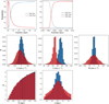 |
Fig. 1 Top panels: probability of stars of belonging to the ks_thick (red), ks_thin (blue) disc, or ks_halo as a function of fraction of stars (left) and a zoom-in of a small fraction of stars to help visualise the halo probabilities (right). Middle panels: velocity components U (left), V (middle), and W (right) distributions of selected ks_thick (red) and ks_thin (blue). Bottom panels: distribution of the heliocentric radius projection over the Galactic plane, R, (left), and distance from the plane, z, (right) of the selected ks_thick (red) and ks_thin (blue). |
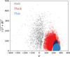 |
Fig. 2 Toomre diagram of the selected ks_thin disc (blue), ks_thick disc (red), and halo (grey) stellar samples considering the quality selection criteria. |
2.3 Derivation of the star formation histories
We derive the deSFHs of the ks_thick and ks_thin discs separately using CMDft.Gaia, which is a suite of procedures specifically designed to perform CMD fitting using Gaia data. This software is presented in great detail in Paper I. Briefly, it comprises three modules performing the main steps required in the total process: (i) ChronoSynth, which computes the synthetic mother CMDs (see Paper I) from a given stellar evolution library; (ii) DisPar-Gaia, that simulates in the mother CMD the observational errors and completeness of the observed one; a complete description of the procedure is presented in the Appendix A of this paper; and (iii) DirSFH, which performs the statistical comparison of the observed CMDs and a large number of model CMDs obtained as linear combination of single stellar populations (SSP; sample of stars covering a small range of age and metallicity) extracted from the mother CMD, searching for the model CMD that best reproduces the observed one, which we will call solution CMD.
We performed the analysis using a mother CMD computed with ChronoSynth based on the solar scaled BaSTI-IAC stellar evolution library (Hidalgo et al. 2018). It contains 120 million stars with MG ≤ 5. A binary fraction β = 0.3; a minimum mass ratio, qmin, between secondary and primary stars equal to 0.1; a Kroupa initial mass function (IMF) (Kroupa et al. 1993) for the primaries; and a flat distribution between qmin × Mp and Mp for the secondaries were adopted. This is the binary parametrisation that was found by Gallart et al. (2024) to best reproduce the magnitude distribution of the stars in the main sequence, below the oMSTO, in the case of the GCNS, and thus we adopted it for this relatively similar sample. The distribution of stellar ages and metallicities in this mother CMD is the one resulting from the assumption that stars are born with a constant probability for all ages and metallicities within the following age and metallicity ranges: 0.02< age <13.5 Gyr and 0.0001<Z<0.039. The total mass of stars formed over 13.5 Gyr that results in the stellar population in this mother CMD at the present time is 1.737341546 × 10⁹ M⊙, and this value is used in the mass normalisation.
To account for the complex observational effects present in Gaia data, we developed DisPar-Gaia, a procedure that mimics these effects in the mother CMD by simulating both uncertainties and incompleteness. DisPar-Gaia assigns observational properties to the synthetic stars based on the distributions from our selected sample, incorporating the extinction (and its error) and photometric uncertainties. It then filters stars according to the Gaia selection function and adds the RVS selection function via empirical completeness masks derived from the ratio of stars with and without radial velocity data. DisPar-Gaia also applies to this updated synthetic CMD the same quality cuts used in the observed data to match real observational constraints. Finally, it perturbs the synthetic absolute magnitudes using propagated uncertainties to fully simulate the observational dispersion seen in Gaia. Specific details can be found in Appendix A of this paper.
Finally, DirSFH is used to find the best-fit parameters. We ran it a total of 64 times, each with a different realisation of the SSPs resulting from de dissection of the mother CMD as a function of age and metallicity using a Dirichlet-Voronoi tessellation scheme. The deSFH provided are the average of the 64 deSFH realisations. S age bins (see Paper I for a definition of the age bins applied) and 0.1 dex metallicity bins have been adopted by DirSFH to define the SSPs. We have also taken into account the small offsets of −0.035 mag and 0.04 mag in (BP − RP) colour and MG magnitude, respectively, between the Gaia photometric system and the BaSTI-IAC theoretical framework in the same photometric passbands (see Paper I for more details). We use a bundle with a faint limit MG=4.1 and weight of each CMD pixel calculated as the inverse of the variance of the stellar ages in that pixel. We note that our analysis is conducted in the absolute magnitude plane, so a good and well characterised completeness is required in absolute magnitude down to the oldest main-sequence turnoff – a condition that is met, aside from the known Gaia incompleteness, which we account for. At a distance of 500 pc, an absolute magnitude MG=4.1 corresponds to G=12.59 (or slightly fainter depending on reddening). As shown in Figure A.1, Gaia is essentially complete in radial velocities down to G ∼ 14, and to G ∼ 12.5 for the bluest stars. By applying an absolute magnitude limit in our analysis, the normalisation – specifically, the fraction of stellar mass outside the bundle – becomes straightforward to compute for a given IMF. We encourage consulting Paper I for deeper insight into the details of the method.
Figure 3 shows the observed CMDs for the ks_thick disc and the ks_thin disc (left panels), with the bundle region used to perform the analysis enclosed by a black polygon. The middle panels show the solution CMDs, derived by selecting stars in the mother CMD with a distribution of age and metallicity given by the best-fit parameters resulting from the average of the 64 best deSFH solutions. Finally number count differences between the observed and the solution CMDs are displayed on the right panels, in units of  in each CMD pixel of size 0.02 × 0.11 mag. We note the overall good match of the solution CMDs, which faithfully reproduce the shapes of the different stellar sequences in the observed CMDs, and also the number counts are consistent within ± 3 σ with no notable systematic residuals in the fitting region. The most noticeable difference between the observed and the solution CMD occurs for the red-giant branch and red-clump region of the ks_thin disc. These two stellar evolutionary phases can be affected, from a theoretical point of view, by non-negligible uncertainties mainly in the effective temperature, as due for instance to the actual efficiency of super adiabatic convection (see, e.g. the discussion in Creevey et al. 2024, and references therein), and to the bolometric corrections used for transferring model predictions from the H-R diagram to the Gaia photometric system. However, we wish to note that these regions of the CMD have a relatively low weight in the overall fit, both due to the lower number of stars compared to the main sequence and to the weighting scheme applied. Outside the bundle, in the main sequence below the old main sequence turn-off, the residuals of the fit exceed 3 σ and show some systematics. We note that in this region, there is a very large density of stars, and any small mismatch in the error simulation, in the slope of the main sequence, or in the reddening corrections can lead to residuals over 3 σ, but these have had no influence in the fit.
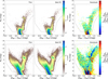 |
Fig. 3 Observed (left) and best-fit solution (middle) CMDs and the residuals (right) for the ks_thick disc (top) and ks_thin disc (bottom). The region used in the fit is plotted enclosed by a black polygon. |
3 Results
In this section we describe the resulting deSFH and AMDs for the local, kinematically selected, Milky Way ks_thick and ks_thin discs, and we will explore their chemical properties based on chemical abundance data from the literature. Owing to radial migration, this local sample is composed both by stars that have formed within its boundaries, and by stars born both at inner and outer radii which are currently inside our volume. Also, a fraction of stars born within the volume boundaries are now outside them. This has to be considered in the interpretation of our findings, and for this reason we use the term deSFH or dynamically evolved star formation rate (deSFR)5 when describing the results.
3.1 The age-metallicity distributions
Our results, displayed in Figure 4, reveal that the ks_thick disc is mainly older than 10 Gyr and underwent a fast chemical enrichment in a short period of time. Its deSFH is characterised by three main episodes of star formation with discontinuities and peaks distributed as follows: one older than 12 Gyr with its maximum of star formation at [Z/H] ∼−0.5 dex, but also with a tail towards lower metallicities at older ages; a second one, that produced most stars in this sample, reaches its peak around 11 Gyr ago and lasts ∼ 1 Gyr while increasing fast in metallicity from [Z/H]=−0.5 to [Z/H]=0.0; and a third one which is very concentrated around ∼ 10.5 Gyr ago and it has already supersolar metallicities. These three main episodes show a reduction in the SFR around [Z/H]=−0.4 and at solar metallicities, approximately. Apart from this major age-metallicity trend, another noticeable peak of star formation stands out in isolation at 6 Gyr and solar metallicity.
Surrounding these main episodes of star formation our analysis returns some other minor populations: for instance, a parallel sequence at slightly lower metallicities and ages younger than the main episodes, following also an increasing metallicity trend as the age decreases down to 8 Gyr; at super-solar metallicities, there is some signal at 13, 10 and 4 Gyr approximately (which will be discussed in an upcoming paper of the same series, Ruiz-Lara et al., in prep.); finally, minor stellar populations younger than 6 Gyr with a wide range of metallicities between −0.5 and 0.5 dex are also visible. The small number of stars in these features prevents us from drawing strong conclusions. Some of these features may result from contamination by ks_thin disc stars, while those with signal-to-noise ratio S/N6 < 10 could be residual artefacts from the analysis.
The ks_thin disc AMD basically starts where those of the ks_thick disc ends, that is, around 10 Gyr ago and with supersolar metallicity. It is narrow down to ∼ 8 Gyr while at younger ages it splits in several populations, increasing the range of metallicity at a particular age as time passes by, with its maximum ∼ 6 Gyr ago. Another interesting characteristic is that the metallicity decreases with age until ∼ 3 Gyr ago, when it starts increasing again. This is contrary to what would be expected from a simple chemical evolution (in a closed box), reflecting the complex evolutionary history of the Milky Way disc that is discussed in detail in Section 4.
In addition to this general trend, some minor stellar groups are also visible. One of them is an old metal-poor population, with [Z/H]<−1, highlighted with contour lines. This population was also observed in the deSFH of the stars within 100 pc of the Sun (Paper I) and has particular interest because there have been several works showing evidence of the existence of low metallicity stars in disc orbits. Their origin is currently under debate since it is puzzling to see stars so metal-poor moving in cool orbits (e.g. Sestito et al. 2020; Fernández-Alvar et al. 2024; Belokurov & Kravtsov 2022; Dillamore et al. 2024; Zhang et al. 2024, Nepal et al. 2024b, among others). We discuss this population in further detail in Section 4. On the metal-rich side, we also see discrete populations of super solar metallicities at 13, 10, 7, 4 and 1 Gyr (Ruiz-Lara et al. in prep), some of them coinciding with those present in our ks_thick disc sample. Between 11 and 10 Gyr we see a minor population connected with the super solar star formation episode but at lower metallicities, which resembles the trend observed in the ks_thick disc at such metallicities and slightly older ages. Finally, at intermediate ages, ∼ 7−6 Gyr, where the maximum spread in metallicity is observed, there is a weak but significant tail of stars with metallicities down to [Z/H] ∼−0.8, which is in line with the classical low metallicity end of the bulk of thin disc stars (Bensby et al. 2004).
An exploration of the systematics linked to the methodology was made and presented in Paper I (Appendix C) where we conducted a comprehensive assessment of different possible sources of uncertainty affecting the determination of stellar ages and metallicities. The tests revealed that, although some systematics would be expected due to the intrinsic parameters adopted in the calculation of the synthetic mother CMD (the choice of stellar evolutionary models, the treatment of binary stars, and assumptions about the IMF) or extrinsic uncertainties (e.g. the effect of reddening), the method can robustly recover the properties of distinct stellar populations (tested with open clusters and synthetic stellar populations at several ages and metallicities) with small systematic shifts, such as slightly overestimating the age in populations older than around 7 Gyr (see their Figure C.6 and C.7). These systematic effects would affect in the same way populations with the same metallicity. Based on these tests, we consider that the results described above are robust.
Figure 5 shows the deSFR for the ks_thick (red) and ks_thin (blue) discs as a function of time, essentially collapsing the [Z/H] dimension from Figure 4. The uncertainties of the deSFR inferred and displayed in Figure 5 are the standard deviation σ of the realisations performed in the analysis. This representation highlights the continuity between the star formation in the ks_thick and ks_thin discs, the fact that star formation is non-zero at early times for both components and that a very high level of star formation is observed at very young ages7. Figure 5 highlights the relative values of the deSFR of both components as defined in this paper. However, displaying the deSFR only as a function of time conceals some of the structure and gaps in the deSFH, which are only apparent when considering the deSFR’s dependence on both age and [Z/H].
We end with a note of caution regarding the interpretation of Figures 4 and 5, emphasizing again that the stars currently in the analysed volume are a mixture of stars formed locally and migrated into it, with a fraction of stars born in-situ also moved outside of it. Therefore, the over densities revealed by our analysis might not be directly interpreted as representative of actual star formation bursts that occurred within the analysed volume. The movement of stars into and out of the volume over time may artificially enhance or reduce the number of stars at a given age and metallicity. However, it is equally true that any increase in stellar mass density associated with a specific age and metallicity implies that stars with those properties must have formed as part of a star formation event somewhere in the Galaxy. In this sense, while we cannot reconstruct the full SFH of either the Galaxy or the volume under study, we do obtain an incomplete, yet informative, snapshot of it.
A more accurate reconstruction of the true galactic SFH would require modelling based on stellar kinematics, by combining our derived deSFH with dynamical models to infer the likely origin of stars in the age-metallicity plane and identify those that may have migrated into the volume; however, such modelling comes with its own limitations, including the assumptions and uncertainties inherent in the adopted dynamical framework. A comprehensive treatment of this is beyond the scope of the present work.
Despite these caveats, what remains robust is that the AMDs of the currently living stars within the volume provide a reliable measurement of the present-day stellar population. This is strongly supported by the close agreement of the metallicity distribution functions (MDFs) shown in both Paper I and in the following Section of the present paper.
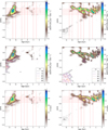 |
Fig. 4 Top panels: dynamically evolved star formation histories, i.e., the stellar mass formed as a function of age and total metallicity ([Z/H]), for the ks_thick (left) and ks_thin (right) discs. Middle panels: same as top panels but including contour lines indicating the signal-to-noise ratio (S/N) of the resulting deSFH. Bottom panels: age and metallicity distribution of living stars in the volume analysed. The colour code indicates now the number of stars per bin in a 100 × 100 grid. In top and bottom panels: red dotted lines mark key age and metallicity values (11, 10, 8, 7, 6, 4 and 3 Gyr) and metallicity values (from 0 to −0.4 in steps of 0.1 dex). The contour lines enclose the 10%, 25%, 50%, 75%, and 95% of M⊙ Gyr−1 dex−1 (top) and the number of stars (bottom) within the age range of 13.5 to 8 Gyr and metallicity range of [Z/H] between −2 and −0.4, highlighting the structure within this region of parameter space. |
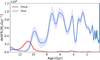 |
Fig. 5 Dynamically evolved star formation rate as a function of stellar age derived with CMDft.Gaia for the ks_thick (red) and ks_thin (blue) discs. Shaded area around each curve represents one standard deviation. |
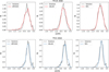 |
Fig. 6 Metallicity distribution functions for the ks_thick disc (top panels) and the ks_thin disc (bottom panels) derived from our solution CMDs compared with those obtained from the spectroscopic surveys APOGEE (left), GALAH (middle), and the Golden Sample of Gaia-RVS (right). The red or blue curves correspond to the spectroscopic MDFs, and the black lines display the MDF distribution from each corresponding masked solution CMD (see text for details). |
3.2 Metallicity distribution functions
Our methodology enables us to determine precise MDFs using photometric data from the Gaia mission, which provides more comprehensive coverage than spectroscopic surveys, overcoming selection biases. The accuracy of the metallicity values can be verified comparing our MDFs with those derived from high-precision spectroscopic measurements such as those obtained from high-resolution spectroscopic surveys such as APOGEE DR17 (Abdurro’uf et al. 2022), GALAH DR3 (Buder et al. 2021), and Gaia RVS (Recio-Blanco et al. 2023). For this purpose, we cross-matched these spectroscopic databases with our ks_thin and ks_thick discs samples. We cleaned them from not reliable abundance determinations following the same criteria applied by Fernández-Alvar et al. (2024). In the case of Gaia RVS we choose the sample provided by Recio-Blanco et al. (2024) (see their Appendix B) that provides an extremely precise stellar chemo-physical parameters and iron abundance (mh_gspspec) measurements with uncertainties lower than 0.05 dex.
It is important to note that these surveys provide measurements of iron abundance, not the total stellar metallicity (i.e. the sum of all elements heavier than helium), even when they use the [M/H] notation to describe them. Therefore, we must calculate the total metallicity from the spectroscopic chemical abundances to make a valid comparison with our metallicity estimates. We estimated the global metallicity [Z/H] from the values of [Fe/H] and [α/Fe] by adopting the rescaling law provided by Salaris et al. (1993), whose coefficients have been updated in Pietrinferni et al. (2021) in order to take into account the updated reference solar heavy element distribution adopted in the BaSTI-IAC stellar library:
![Mathematical equation: $[\mathrm{Z} / \mathrm{H}]=[\mathrm{Fe} / \mathrm{H}]+\log \left(0.694 \times 10^{[\alpha / \mathrm{Fe}]}+0.301\right).$](/articles/aa/full_html/2025/12/aa53814-25/aa53814-25-eq7.png) (4)
(4)
To perform the comparison appropriately, we replicated the selection function of these spectroscopic surveys on the solution CMD. In each bin of colour and magnitude across the solution CMD, we randomly selected a number of stars matching the fraction observed by each spectroscopic survey relative to the Gaia photometric observations. We call the resulting CMD the masked solution CMD. We calculated a masked solution for each of the spectroscopic surveys explored. A more detailed explanation of the procedure and an example of a masked solution can be found in Appendix B.
Figure 6 shows the spectroscopic measurements from each of the three databases evaluated (in red or blue, for ks_thick and ks_thin discs, respectively) with the MDFs inferred from our methodology after applying the mask (in black), both normalised to the total area under the curve. The shape of the MDF changes from one survey to another due to the differences of the selection functions. The comparison shows a very good agreement, with the peak and dispersion of our resulting MDF following closely the spectroscopic ones. This manifests (i) that our metallicity estimations have similar precision to the independent and reliable measurements from high-resolution spectroscopic surveys; (ii) that the metallicity scales are also very similar; and (iii) that the solution CMD has been properly treated to take into account the incompleteness of each spectroscopic survey. Our ks_thin disc MDF seems to be affected by a very small [Z/H] offset, with a deficiency of super solar metal-rich stars and an excess in the sub-solar metallicity side. Apart of this small difference, the comparison confidently assures that our metallicity values are reliable and in the same scale.
Figure 6 also shows that the ks_thick disc MDF is broader than the ks_thin disc MDF, extended down to [Z/H] ≤−1.5 with a peak at [Z/H] ∼−0.25, approx., which corresponds to a [Fe/H] ∼ −0.5 since this population is α-enriched. The ks_thin disc has its maximum at [Z/H] ∼ 0 and extends down to [Z/H] ∼−1, although there are also a few stars down to [Z/H] ∼−2. On their metal-rich side, both the ks_thick and the ks_thin disc MDFs reach super solar metallicities.
3.3 The [α / Fe] distribution of the Milky Way discs across time
After confirming that our metallicity scale aligns well with the spectroscopic scales, we evaluate the [α/Fe] distribution observed for stars in the spectroscopic surveys with the age distributions obtained in this work at the same metallicity bins where we see particular episodes of star formation. We evaluate the masked solution to compare the same fraction of stars in the age-metallicity space with the ones observed spectroscopically in the [α/Fe] versus [Z/H] space.
We perform this comparison using abundances from APOGEE and GALAH, with the latter transformed to the APOGEE scale through the SpectroTranslator8 methodology, recently introduced by Thomas et al. (2024). We focus on the [Mg/Fe] versus [Z/H] distribution, as magnesium (Mg) is the element that best distinguishes the two [α/Fe] trends observed in the Milky Way disc. After applying the recommended flags, we cross-match our spectroscopic sample with the one that we use to derive the deSFH, resulting in 519 and 13582 stars in common with our ks_thick and ks_thin disc samples, and with reliable chemical abundances in the APOGEE scale from SpectroTranslator. The Gaia RVS extremely precise sample of stellar chemo-physical parameters sample lacks sufficient Mg abundance determinations to draw robust conclusions, so we limit our analysis to the SpectroTranslator abundances.
Figure 7 shows, on the left, our AMDs, now with the metallicity on the x-axis and age on the y-axis, obtained from the masked solution CMD corresponding to the APOGEE+GALAH SpectroTranslator sample. In these plots we are representing individual stars (top, ks_thick) or stellar density (bottom, ks_thin) of the masked solution CMD. Plots on the right show the [Mg/Fe] versus [Z/H] distribution, represented with red dots in the case of the ks_thick disc and with a density colourmap in blue for the ks_thin disc (because of the larger number of stars). The isocontours in blue (red) display the 30, 60 and 90% percent of the stellar distribution in the chemical space corresponding to the ks_thin disc (ks_thick disc) on top of the ks_thick disc (ks_thin disc) stars. These plots highlight the fact that the kinematically selected ks_thick and ks_thin discs do not correspond exactly to the chemically selected thick and thin discs, i.e. they do not result in the typical clean chemical separation between high- α and low- α populations.
The ks_thick disc main episodes of star formation cover three distinct well defined metallicity ranges: [Z/H]<−0.35,−0.35< [Z/H]<0.1, and [Z/H]>0.1. We split the sample in these ranges in order to evaluate the [Mg/Fe] abundances separately for each of them. The [α/Fe] abundances of the oldest (>12 Gyr) ks_thick disc stars are overall high α. The metallicity range covered by the most prominent epoch of star formation between 12 and 10 Gyr ago (−0.35<[Z/H]<0.1), shows a very large [Mg/Fe] dispersion, although the contour lines corresponding to the ks_thick disc (over-imposed on the ks_thin disc plot) reveal that a majority of the stars in this range have high [Mg/Fe] and also a global decreasing trend of [Mg/Fe] as a function of metallicity from a high- α plateau down to [Mg/Fe] ∼ 0 at [Z/H] ∼ 0. Finally, the third population at super solar metallicites is characterised by solar [Mg/Fe] abundances.
A high- α plateau followed by a decreasing [Mg/Fe] while metallicity increases is a chemical trend well explained by the chemical enrichment of the gas by SNe with a massive star progenitor contributing early at low metallicities, and then by low-mass stars exploding as SNIa later, increasing the metallicity while the [Mg/Fe] ratio decreases (Matteucci & Greggio 1986). Our results clearly show that the Milky Way started forming stars very early and enriched the ISM very fast: approximately 12 Gyr ago, the Milky Way had reached already a metallicity of [Z/H] ∼−0.5 and, based on their high- α abundance ratios, most of the stars did not have received yet the contribution of the nucleosynthetic products of low-mass stars.
Even though most stars born in the second epoch (12–10 Gyr ago) are α-rich, the decrease in [Mg/Fe] is noticeable already at [Z/H] ∼−0.35, i.e. at ages younger than 12 Gyr. This indicates that after ≃1.5 Gyr of star formation there would have been enough time for SNIa from low-mass stars to explode and enrich the ISM with Fe. However, the “knee” of this population is not well-defined. This may be due in part to uncertainties in spectroscopic metallicities. But we also note that a number of intermediate-age stars with age ≃6 Gyr old and solar metallicities, which would have a low- α signature, enter in this metallicity range and increase the dispersion of [Mg/Fe]. Additionally, we propose that the observed dispersion in both metallicity and [Mg/Fe] could have a physical origin related to the Milky Way’s accretion history during this period. If the Milky Way accreted a satellite galaxy at this time, the mixing of gas and stars could have enhanced the variability in metallicity and α element abundances of the stars formed afterward. We explore this scenario in more detail in Section 4. Lastly, the chemical analysis of the most metal rich episode of star formation in the ks_thick disc shows that 10 Gyr ago the Milky Way already reached super-solar metallicities and low- α ratios.
The deSFH of the ks_thin disc is more complex, with star formation episodes at several metallicities overlapping in age. We again compare the AMD with the [Mg/Fe] versus [Z/H] trend in ranges of metallicity. As mentioned earlier, the majority of the ks_thin disc began forming 10 Gyr ago, already exhibiting super-solar metallicities. The comparison with the [Mg/Fe] versus [Z/H] trends shows that these stars correspond to the metal-rich tip of the low- α sequence or chemical thin disc. The bulk of these stars show an overall [α/Fe] ∼ 0, with some dispersion ranging between −0.1 and 0.1. This metallicity range is also populated by the youngest star formation and the very metal-rich discrete populations observed at different ages.
As mentioned above, the ks_thin disc age-metallicity trend decreases in metallicity as time goes by, up to around 4−3 Gyr ago when the metallicity increases again. At the same time, there is an overlap of stellar populations with different metallicities at the same age. Or equivalently, at a particular metallicity range there are stellar populations covering a broad range of ages. This is specially the case for the metallicity range between −0.35<[Z/H]<0, in which there are stars ranging from 11 Gyr to the youngest ones. At the same time there is a very large dispersion in [Mg/Fe], from sub-solar up to thick-disc-like high- α ratios. This large spread might be explained by the superposition of these several populations at different ages that evolved differently with time and, consequently, reached distinct [Mg/Fe] ratios at the same [Z/H]. In particular, it seems that the stars with the highest [Mg/Fe] ratios correspond to stars between 11 and 10 Gyr old, if we consider the comparison with the thick-disc chemical trend.
Lower metallicities correspond to the low metallicity tip of the low- α sequence or chemical thin disc. Traditionally, the metal-poor boundary of the thin disc has been set around [Fe/H] ∼−0.7, equivalent to [Z/H] ∼−0.6 when considering [Mg/Fe] ∼ 0.1. Stars ranging between −0.6<[Z/H]<−0.35 show a moderate α enhancement, mostly concentrated at [Mg/Fe] ∼ 0.1, following a decreasing [Mg/Fe] trend with increasing [Z/H]. In our age-metallicity space, these stars clearly cover an age range between 7 and 3–2 Gyr.
Recently, several studies have provided increasing evidence for stars in thin-disc-like orbits with metallicities below [Z/H] ≃−0.6 (e.g. Sestito et al. 2019; Sestito et al. 2020; Sestito et al. 2021; Fernández-Alvar et al. 2021; Fernández-Alvar et al. 2024; Yuan et al. 2024; Bellazzini et al. 2024; Nepal et al. 2024b; González Rivera de La Vernhe et al. 2024; although see also Zhang et al. 2024). Our findings support these results, as our analysis also identifies stellar populations with [Z/H]<−0.6 and even [Z/H]<−1. In our AMD, these metal-poor stars correspond to old and intermediate-age stars, spanning an age range from approximately 13.5 Gyr down to around 8 Gyr([Z/H]<−1) and around 5−4 Gyr([Z/H]<−0.6), drawing a trend of increasing metallicity with age. Interestingly, despite the similar age-metallicity trend, there appears to be a gap or disconnection between stars older than 8 Gyr and those younger, which could suggest a different origin for stars with metallicities above and below −1. However, the limited number of stars in our sample prevents us from drawing a definitive conclusion. The [Mg/Fe] versus [Z/H] plot only shows a handful of these stars, some with high- α ratios and others with lower- α content. The only star with [Z/H]<−1 is most likely older than 10 Gyr as has a clear high- α ratio. The apparent discrepancy in the number of low metallicity stars ([Z/H] < −0.6) inferred from our deSFH and that in the spectroscopic sample may have a number of causes and its origin is beyond the scope of this work. The fraction of stars in this metallicity range on our solution is very small (2.5% of the total ks_thin disc), but their presence seems to be a robust finding (this tail of low metallicity stars is also found in the deSFH for the 100 pc sample studied by Gallart et al. 2024), which is discussed in detail by Queiroz et al. (in prep). While it is usually assumed that these stars are old based on their low metallicity, in this work we are actually confirming this assumption by dating this stellar population.
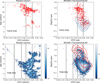 |
Fig. 7 Left panels: age-metallicity distribution of the masked solutions for ks_thick disc stars (top, represented by individual red points) and ks_thin disc stars (bottom, shown as a blue-scale hexbin density diagram). This is the same solution as Figure 4 bottom panels, i.e., the distribution of synthetic stars from the best fit which corresponds to the age-metallicity distributions of the living stars in the volume analysed. Right panels: [Mg/Fe] versus [Z/H] (global metallicity; see Section 3.2 in the main text) based on spectroscopic measurements from APOGEE DR17 and GALAH DR3, homogenised using the SpectroTranslator. The ks_thick disc stars are displayed at the top (with individual red points), while ks_thin disc stars appear at the bottom (as a blue-scale hexbin density diagram). The isocontours in red (blue) display the 30%, 60%, and 90% percent of the stellar distribution in the chemical space corresponding to the ks_thin disc(ks_thick disc) in addition to the ks_thick disc(ks_thin disc) stars. The vertical black dashed lines indicate the metallicity ranges of interest discussed in the main text. |
4 Discussion
4.1 The ks_thick disc star formation history
This work clearly demonstrates that the ks_thick disc formed very early, around 13 Gyr ago, undergoing rapid metallicity enrichment and reaching supersolar values approximately 10 Gyr ago, at which point subsequent star formation in the Milky Way disc appears to have occurred in colder, thin-disc-like orbits. This is not the first time that evidence in this sense has been presented. Based on ages inferred from exquisite asteroseismic constraints on RGBs observed by APOGEE Miglio et al. (2021) showed that the chemical thick disc, i.e. the α-rich population, has ages around 11 Gyr with an spread of ∼ 1.5 Gyr. Xiang & Rix (2022) published an age-metallicity relation for Milky Way stars, derived from LAMOST subgiant stars, for which precise individual stellar ages could be determined. Their results also indicated that the thick disc9 began forming about 13 Gyr ago, with the majority of its stars being approximately 11 Gyr old. Similarly, Sahlholdt et al. (2022) analysed GALAH DR3 main sequence turn-off and subgiant stars, finding that the kinematically hot stars formed along a single age-metallicity sequence, which ended around 10 Gyr ago, when the low- α sequence began forming and stars with lower vertical dispersions became dominant. Finally, Queiroz et al. (2023) show that the chemical thick disc for LAMOST, APOGEE and GALAH peak at approximately 11.3 Gyr with a dispersion of 1.5 Gyr. Recently, Cerqui et al. (2025) analysed age-abundance relations for a sample of 30 000 dwarf stars from APOGEE DR17 within 2 kpc of the Sun, finding a rapid increase in [Fe/H] and a decrease in [α/Fe] with decreasing age down to ∼ 8 Gyr. Their chemical trends agree with ours, although we find a faster evolution concluding around 10 Gyr ago. Accounting for their acknowledged age uncertainties of up to 2 Gyr, their results are consistent with ours.
However, our AMD exhibits significantly less dispersion at a given age compared to those inferred based on individual star age determinations (see also figures 13, C.3, C.4 and C.7 in Paper I). This, together with the large statistics in our samples10, allows revealing details hidden within the uncertainties in previous studies, such as the fact that the ks_thick disc experienced three distinct episodes of star formation, centred approximately 12, 11, and 10.5 Gyr ago, with the most significant peak occurring around 11 Gyr ago. Additionally, and unlike in these previous studies, our AMD can be considered virtually complete, as the very mild incompleteness that affects our stellar sample has been carefully simulated in the mother CMD as discussed in Appendix A. Finally, the deSFH shown in Figure 4 accounts for all stellar mass formed throughout time, including stars that are no longer present due to having completed their life cycles.
Figure 4 shows that the ks_thick disc appears to have experienced its last major star formation episode around 10.5 Gyr ago, coinciding with the timing of the last major merger in the Galaxy: the accretion of the Gaia-Sausage-Enceladus (GSE) galaxy (Belokurov et al. 2018; Helmi et al. 2018; Vincenzo et al. 2019; Di Matteo et al. 2019; Gallart et al. 201911; Bonaca et al. 2020; Montalbán et al. 2021). Cosmological simulations predict that the accretion of galaxies can trigger star formation in both the host galaxy and the accreted satellite (Di Cintio et al. 2021; Orkney et al. 2022). The pericentre passages of the accreted satellite compress the gas in the host galaxy through gravitational interactions. This compression increases the gas density leading to conditions favourable for star formation, with peaks aligning with the pericentric passages of the satellite.
Given this, it is plausible that the GSE accretion also stimulated star formation in the proto-Milky Way. Therefore, we speculate that the star formation episodes observed in the ks_thick disc around 11 and 10.5 Gyr ago may be linked to the GSE merger. Queiroz et al. (2023) concluded that the high-[α/Fe] population, which they call the genuine thick disc, formed before the GSE accretion. In our study the high-[α/Fe] population would be the first star formation episode (≤ 12 Gyr), and probably part of the second one (∼ 11 Gyr). The metallicity range cover by the second and third star formation events show a significant dispersion in [α/Fe], yet an overall decrease in [α/Fe] with increasing [Z/H] within a relatively narrow [Z/H] range. Two and a half Gyr of chemical evolution could be in principle sufficient to lower the [α/Fe] abundances and produce a well defined ‘knee’ in the [α/Fe] versus [Z/H] chemical space; however, we did not observe a clearly defined ‘knee’. Yet, if these starbursts were triggered by a pericentre passage of GSE, leading to the accretion of more metal-poor gas from this satellite into the Milky Way, the newly accreted gas would dilute the pre-existing metal-enriched gas. This dilution would result in a slower overall metallicity increase, counteracting the rise in Fe from Type Ia supernova explosions. Additionally, the starburst would lead to the formation of new massive stars, which would quickly explode as supernovae, keeping the [α/Fe] relatively high and likely contributing to the observed abundance dispersion.
Belokurov & Kravtsov (2022) analysed the azimuthal velocity spin-up of stars within the APOGEE DR17 and Gaia DR3 databases to conclude that the transition from halo to thick disc orbits occurred between −1.3<[Fe/H]<−0.912, after what the Galaxy settles into a coherently rotating thin disc. We see that the first high peak of star formation occurred ∼ 12 Gyr ago with a metallicity of [Z/H] ∼−0.5, but we also detect a tail towards lower metallicities down to at least [Z/H]<−1 at ages <13 Gyr. We are thus identifying in our deSFH a well-defined event of star formation that can be associated with that early disc component, and thus we are able to date this spin-up as having occurred indeed very early on in the history of the Galaxy, around 12 Gyr ago, or even earlier.
Another intriguing feature in the upper panel of Figure 4 is the sharp peak of star formation around 6 Gyr ago. This coincides with the estimated timing of the first pericentre passage of the Sagittarius dwarf galaxy (Law & Majewski 2010; Laporte et al. 2018). As previously suggested, such a passage could have triggered star formation in the Milky Way, as other studies have also proposed (Ruiz-Lara et al. 2020). By this time, the ks_thin disc was already established, as indicated by its SFH. The observation of this stellar population in orbits characteristic of the ks_thick disc suggests that stars (or the gas from which these stars formed) may have been heated during the merger with the Sagittarius dwarf galaxy, contributing to the observed stars with kinematic characteristics of the ks_thick disc. This is similar to the explanation proposed by Gallart et al. (2019) and Belokurov et al. (2020) to account for star with chemically thick-disc-like properties found in halo orbits.
The presence of young stars (ages <8 Gyr) in the ks_thick population might also be attributed to the phenomenon of young alpha-rich stars (Chiappini et al. 2015; Martig et al. 2015; Grisoni et al. 2024). Such stars, characterised by high abundances of alpha elements and young apparent ages, have been identified in multiple datasets and exhibit kinematics consistent with those of thick disc stars (Silva Aguirre et al. 2018; Lagarde et al. 2021; Queiroz et al. 2023). This phenomenon is likely a consequence of mass accretion in binary systems (Jofré et al. 2016, 2023), which can cause stars to appear younger than their true ages.
4.2 The transition from the ks_thick disc to the ks_thin disc
The majority of the ks_thin disc’s stellar content spans from 10 Gyr ago to the present. Notably, ks_thin disc stars began forming at the same time and metallicity at which the ks_thick disc halted its primary star formation-around 10 Gyr ago, at slightly super solar metallicities. Even more intriguingly, this transition from ks_thick to ks_thin disc formation coincided with the time range inferred by most studies for the accretion of GSE (Belokurov et al. 2018; Helmi et al. 2018; Vincenzo et al. 2019; Di Matteo et al. 2019; Gallart et al. 2019; Bonaca et al. 2020; Montalbán et al. 2021). Our findings suggest that sustained star formation in the settled ks_thin disc could only begin after the last major merger had concluded, ushering in a more stable period. This provides independent evidence for the timing of the Milky Way’s last major merger. We also observe that the transition from ks_thick to ks_thin disc orbits occurred at supersolar metallicities, corresponding to the metal-rich end of the low- α stellar population. This was already pointed out by Haywood et al. (2013) were they showed that the oldest stars of the chemical thin disc have a metallicity as high as the youngest stars of the chemical thick disc, and a subsequent increase in metallicity dispersion is found for younger thin disc stars.
However, there are also a small fraction of stars with high-α abundances that exhibit thin-disc kinematics. The fact that these stars are slightly older than 10 Gyr suggests they could be among the earliest formed in thin-disc-like orbits, during a period when the Galaxy was accumulating angular momentum. Anders et al. (2018) and Ciucă et al. (2021) discuss a chemically distinct population often referred to as ‘transition’ or ‘bridge’ stars, which exhibit chemical abundances that fall between those of the chemical thin and thick disc populations. These stars are more prevalent in the inner regions of the galaxy. The earlier formation phase that we detect in the ks_thin disc in the metallicity range where we observe a large range of [Mg/Fe] could potentially be linked to the chemically identified transition population, reflecting a significant period of disc evolution when these ‘bridge’ stars emerged.
Although the majority of the ks_thin disc stars have ages younger than 10 Gyr, our analysis also reveals the presence of very old stars (age >12 Gyr) with both very low ([Z/H] < −1) and very high metallicities ([Z/H] > 0). This finding is consistent with previous reports of very old, metal-rich stars (Nepal et al. 2024b, Recio-Blanco et al. 2024) and the already discussed presence of very metal-poor stars. However, these populations appear disconnected from the bulk of the ks_thin disc stars, suggesting they may have a different origin than the majority of the ks_thin disc present in the analysed volume, whose older populations are linked to the transition from thick to thin orbits.
4.3 The ks_thin disc star formation history
The deSFHs inferred represent that of the stars currently present in the solar neighbourhood. Stars on cool orbits, such as those in the ks_thin disc, are more influenced by radial migration than stars on ks_thick disc orbits. As a result, many of these stars were likely born in different regions of the Galaxy (Haywood 2008; Minchev et al. 2013; Minchev et al. 2014). Radial migration is expected to have brought stars from distant locations, preferentially the inner regions. Also, stars do not move in perfectly circular orbits but also stars from both the inner and outer disc might be crossing the solar radius at the present time as they reach their apocentres and pericentres. Therefore, the SFH inferred from ks_thin disc stars reflect star formation not only in the solar neighbourhood but also in the regions where these migrated stars originally formed.
Previous analysis of the stellar and interstellar medium abundances across the thin disc have demonstrated a metallicity gradient with respect to galactocentric distance, with the inner regions being more metal-rich than the outer regions (Tissera et al. 2016; Esteban & García-Rojas 2018; Lemasle et al. 2018; Méndez-Delgado et al. 2022; Lian et al. 2023; Carbajo-Hijarrubia et al. 2024). However, one of the characteristic signatures of radial mixing is the presence of substantial metallicity dispersion at a given radius (Haywood 2008; Minchev et al. 2013). The ks_thin disc deSFH inferred from our analysis shows distinct star formation episodes at several metallicities overlapping in age, which increase the total metallicity range and hint to the superposition of several stellar populations. This is specially noticeable between 8 and 3 Gyr ago and suggests the presence in the studied volume of stars that have migrated from different regions of the Galaxy, each having undergone distinct SFHs. For ages younger than 3 Gyr, the metallicity dispersion decreases, consistent with the notion that these younger stars have had less time to migrate, and that less mergers inducing star formation and migration have occurred at later times.
Based on the observed interstellar medium gradient (Méndez-Delgado et al. 2022) and assuming that a qualitatively similar gradient has been present over the lifetime of the Milky Way, we would expect that the most metal-rich stars in our sample originated from the inner disc, while the metal-poor stars came from the outer disc. Consequently, the inferred decrease in metallicity with decreasing age, which seems to hold for the two main metallicity branches, may result from the combined effect of the inside-out growth of the disc and the radial mixing between stars from inner and outer radii. Similar conclusions have been drawn by Xiang & Rix (2022), Sahlholdt et al. (2022) and Gallart et al. (2024), who highlighted the role of migrating stars in shaping their derived age-metallicity relations. In this scenario, the lowest metallicity populations, extending between 8−7 and 3 Gyr ago, can be used to constrain the epoch of formation of the outer disc, indicating it cannot be older than 8 Gyr, as an earlier formation would have allowed time for these stars to migrate to the solar neighbourhood.
An alternative explanation has been proposed by Haywood et al. (2024) and Zhang et al. (2025). They suggest that resonant dragging by the co-rotation resonance of a decelerating bar could be responsible of the observational radial metallicity profile and its trend with guiding radius and the double age-metallicity sequence observed in the solar neighbourhood. In their scenario, the more metal-rich sequence consists of stars born in the inner Galaxy and later displaced outwards by this dynamical mechanism, which aligns with our hypothesis that the metal-rich branch likely originated in the inner regions. In addition, Zhang et al. (2025) interpret the lower-metallicity sequence as representing the local stellar population based on the comparison with a test-particle simulation, although they also caution that her assumption of a constant bar strength may lead to an overestimation of the efficiency of stellar migration.
Renaud et al. (2021b), Renaud et al. (2021a) presented an interesting scenario for the possible formation of the outer disc around 8 Gyr ago, based on their analysis of the Vintergatan simulation (Agertz et al. 2021). This simulation, which models a Milky Way-like galaxy, presents an [α/Fe] dichotomy and multiple branches in the age-metallicity plane, similar to the ones observed in our Galaxy. According to the simulation, star formation in the outer disc was triggered when a satellite galaxy began merging with a Milky Way-like galaxy (Vintergatan) along a filament. The tidal forces associated with this gravitational interaction compressed gas in the outer disc, thereby boosting star formation, which occurred at a lower [Fe/H] compared to the inner disc that had already been previously enriched in an epoch characterised by frequent merger events. Renaud et al. (2021b), Renaud et al. (2021a) demonstrated how this last major merger initiated the formation of the outer disc, the low- α sequence, and the ks_thin disc. They predicted that this process would result in a dichotomy of [Fe/H] at around 8 Gyr ago, corresponding to the low and high metallicity ends of the low- α sequence.
As predicted by the Vintergatan simulation our results indicate a clear split in [Z/H] around 8-7 Gyr ago. However, we also infer the presence of stars with ks_thin disc kinematics but super solar metallicities 11−10 Gyr ago, the approximate time when the chemistry of the stars transitions from high to solar-like [α/Fe] abundances. This suggests that star formation in thin disc orbits began in the inner regions earlier than in the outer disc. Unlike in the Vintergatan simulation, here the onset of the α-poor population and the appearance of the low metallicity branch seem to be disconnected, maybe pointing to more than one merger event as responsible. We have already discussed the likely relation between the GES merger and the ks_thick-ks_thin disc transition occurring ≃10 Gyr ago. The emergence of the lowest metallicity branch around 8−7 Gyr ago could be linked to a different merger event, possibly that of the Helmi Streams, dated to have occurred around that time (Kepley et al. 2007; Koppelman et al. 2019; Ruiz-Lara et al. 2022), while later signatures (e.g. the ks_thick disc stellar overdensity and clearly defined double branch 6 Gyr ago, or the features at three different metallicities 4 Gyr ago) could point to the Sgr dwarf accretion as the culprit (Ruiz-Lara et al. 2020; Gallart et al. 2024). It is important to note, however, that our sample consists of stars currently populating a volume of radius 250 parsecs around the Sun, which may not adequately represent the outer disc. This limitation affects our ability to provide a robust characterisation of that region.
The observed bifurcation of stellar populations in [Z/H] as a function of time is likely the result of multiple dynamical processes that have shaped the diverse stellar content of the solar neighbourhood. The current challenge lies in disentangling the relative contributions of each of these processes to the present-day stellar distribution.
5 Summary and conclusions
We have derived the dynamically evolved deSFHs of the ks_thick and ks_thin discs, selected according to position and kinematics, within a cylindrical volume with a radius of 250 pc and a height of 1 kpc centred on the Sun. These results provide unprecedented insights into the star formation and evolution of the ks_thick and ks_thin discs. While confirming previous findings, they also crucially resolve lingering questions about specific star formation episodes, their duration, their associated chemical enrichment, and the timing of the transition from thick to thin disc kinematics. Our main conclusions are summarised as follows:
- (i)
Our results show that the ks_thick disc is primarily older than 10 Gyr and experienced rapid metallicity enrichment in a short period. Its SFH reveals three key episodes: (i) the first, older than 12 Gyr ago, peaked at [Z/H] ∼−0.5 dex and allows for quantitative dating of the first time the very early disc spunup, which occurred over 12 Gyr ago. (ii) A second, more intense episode occurred around 11 Gyr ago, with the metallicity quickly rising from [Z/H]=−0.5 to 0.0. Finally, a third short period took place just over 10.5 Gyr ago at supersolar metallicities;
- (ii)
Most of the ks_thin disc stars began forming around 10 Gyr ago with super solar metallicity and low [α/Fe] content. Our analysis indicates that the low- α sequence started at super solar metallicities around 10 Gyr ago and extended to its metalpoor end ([Z/H] ∼−0.8) by 8−7 Gyr ago. Stars at intermediate metallicities span ages from 10 Gyr ago to the present time;
- (iii)
There is a minor population of ks_thin disc stars with high α abundances that are slightly older than 10 Gyr. This result evidences that when the Galaxy was transitioning from high α to low α and from sub-solar to super-solar metallicities between 11 and 10 Gyr ago, a kinematical transition was happening, too. This transition coincides with the estimated epoch at which the Milky Way underwent its last major merger with the accretion of GSE;
- (iv)
The age-metallicity relation of the ks_thin disc remains narrow until about 8 Gyr ago, after which it diverges into overlapping star formation episodes at the same age with distinct metallicities, likely indicative of radial mixing. This leads to an increased metallicity range that peaks around 6 Gyr ago. Given that stars in the low-metallicity branch likely originated in the outer disc, our results suggest the outer disc formed around 8 Gyr ago, possibly coinciding with subsequent merger events;
- (v)
The average ks_thin disc metallicity started to increase approximately 3 Gyr ago, likely reflecting the true local chemical enrichment since stars may not be able to migrate substantially in such a short period of time. Additionally, no substantial merger events have occurred in this period of time;
- (vi)
Our analysis also uncovered minor populations within the ks_thick and ks_thin disc that appear disconnected from the main age-metallicity trends, echoing similar findings in the literature. These include (i) a very old (age >10 Gyr), metal-poor ([Z/H] < −1) stellar population with ks_thin disc kinematics; (ii) a notable 6 Gyr old population with solar metallicity and ks_thick disc kinematics, possibly associated with the first pericentre of the Sagittarius satellite galaxy; (iii) several distinct populations of very metal-rich ([Z/H] ∼ 0.5) stars with various ages (consistent with recent findings (Nepal et al. 2024a; Recio-Blanco et al. 2024)), which likely migrated from the inner galaxy.
The exquisite details in the deSFH of the ks_thick and ks_thin discs clarify unresolved questions regarding the specific star formation episodes that occurred in both discs, their duration, and consequent chemical enrichment, and they allowed us to date the kinematic settlement of the Milky Way disc. These results constitute important observational constraints that need to be contrasted with chemical evolution models and cosmological simulations in order to understand the physical processes that led to such SFH characteristics. Further papers in this series will continue to exploit the ability of CMDft.Gaia to dissect the Milky Way as never before.
Acknowledgements
We thank R. Lallement and G. Green for useful discussions regarding the use of their respective extinction maps. EFA acknowledges support from HORIZON TMA MSCA Postdoctoral Fellowships Project TEMPOS, number 101066193, call HORIZON-MSCA-2021-PF-01, by the European Research Executive Agency. EFA, CG, ABQ, GB and GT also acknowledges support from the Agencia Estatal de Investigación del Ministerio de Ciencia e Innovación (AEI-MCINN) under grants “At the forefront of Galactic Archaeology: evolution of the luminous and dark matter components of the Milky Way and Local Group dwarf galaxies in the Gaia era” with references PID2020-118778GB-I00/10.13039/501100011033 and PID2023-150319NB-C21/10.13039/501100011033. TRL acknowledges financial support by the research projects AYA2017-84897-P, PID2020-113689GB-I00, and PID2020-114414GB-I00, financed by MCIN/AEI/10.13039/501100011033, the project A-FQM-510-UGR20 financed from FEDER/Junta de Andalucía-Consejería de Transformación Económica, Industria, Conocimiento y Universidades/Proyecto and by the grants P20-00334 and FQM108, financed by the Junta de Andalucía (Spain), as well as Juan de la Cierva fellowship (IJC2020-043742I). SC acknowledges financial support from PRIN-MIUR-22: CHRONOS: adjusting the clock(s) to unveil the CHRONO-chemo-dynamical Structure of the Galaxy” (PI: S. Cassisi) funded by European Union – Next Generation EU, and Theory grant INAF 2023 (PI: S. Cassisi). AH and ED acknowledge financial support from a Spinoza grant.
References
- Addurro’uf, Accetta, K., Aerts, C., et al. 2022, ApJS, 259, 35 [NASA ADS] [CrossRef] [Google Scholar]
- Adibekyan, V. Z., Sousa, S. G., Santos, N. C., et al. 2012, A&A, 545, A32 [NASA ADS] [CrossRef] [EDP Sciences] [Google Scholar]
- Agertz, O., Renaud, F., Feltzing, S., et al. 2021, MNRAS, 503, 5826 [NASA ADS] [CrossRef] [Google Scholar]
- Anders, F., Chiappini, C., Santiago, B. X., et al. 2018, A&A, 619, A125 [NASA ADS] [CrossRef] [EDP Sciences] [Google Scholar]
- Aparicio, A., & Gallart, C., 2004, AJ, 128, 1465 [NASA ADS] [CrossRef] [Google Scholar]
- Bellazzini, M., Massari, D., Ceccarelli, E., et al. 2024, A&A, 683, A136 [NASA ADS] [CrossRef] [EDP Sciences] [Google Scholar]
- Belokurov, V., & Kravtsov, A., 2022, MNRAS, 514, 689 [NASA ADS] [CrossRef] [Google Scholar]
- Belokurov, V., Erkal, D., Evans, N. W., Koposov, S. E., & Deason, A. J., 2018, MNRAS, 478, 611 [Google Scholar]
- Belokurov, V., Sanders, J. L., Fattahi, A., et al. 2020, MNRAS, 494, 3880 [Google Scholar]
- Bensby, T., Feltzing, S., & Lundström, I., 2003, A&A, 410, 527 [CrossRef] [EDP Sciences] [Google Scholar]
- Bensby, T., Feltzing, S., & Lundström, I., 2004, A&A, 421, 969 [NASA ADS] [CrossRef] [EDP Sciences] [Google Scholar]
- Bernard, E. J., 2018, in IAU Symposium, Vol. 330, Astrometry and Astrophysics in the Gaia Sky, eds. A. Recio-Blanco, P. de Laverny, A. G. A. Brown, & T. Prusti, 148 [Google Scholar]
- Bernard, E. J., Aparicio, A., Gallart, C., Padilla-Torres, C. P., & Panniello, M., 2007, AJ, 134, 1124 [Google Scholar]
- Bernard, E. J., Schultheis, M., Di Matteo, P., et al. 2018, MNRAS, 477, 3507 [CrossRef] [Google Scholar]
- Bertelli, G., & Nasi, E., 2001, AJ, 121, 1013 [NASA ADS] [CrossRef] [Google Scholar]
- Bland-Hawthorn, J., & Gerhard, O., 2016, ARA&A, 54, 529 [Google Scholar]
- Bonaca, A., Conroy, C., Cargile, P. A., et al. 2020, ApJ, 897, L18 [NASA ADS] [CrossRef] [Google Scholar]
- Bovy, J., Rix, H.-W., & Hogg, D. W., 2012, ApJ, 751, 131 [NASA ADS] [CrossRef] [Google Scholar]
- Bovy, J., Rix, H.-W., Schlafly, E. F., et al. 2016, ApJ, 823, 30 [NASA ADS] [CrossRef] [Google Scholar]
- Brook, C. B., Kawata, D., Gibson, B. K., & Freeman, K. C., 2004, ApJ, 612, 894 [NASA ADS] [CrossRef] [Google Scholar]
- Buder, S., Sharma, S., Kos, J., et al. 2021, MNRAS, 506, 150 [NASA ADS] [CrossRef] [Google Scholar]
- Cantat-Gaudin, T., Fouesneau, M., Rix, H.-W., et al. 2023, A&A, 669, A55 [NASA ADS] [CrossRef] [EDP Sciences] [Google Scholar]
- Carbajo-Hijarrubia, J., Casamiquela, L., Carrera, R., et al. 2024, A&A, 687, A239 [NASA ADS] [CrossRef] [EDP Sciences] [Google Scholar]
- Cerqui, V., Haywood, M., Snaith, O., Di Matteo, P., & Casamiquela, L., 2025, A&A, 699, A277 [NASA ADS] [CrossRef] [EDP Sciences] [Google Scholar]
- Chaplin, W. J., & Miglio, A., 2013, ARA&A, 51, 353 [Google Scholar]
- Chiappini, C., Matteucci, F., & Gratton, R., 1997, ApJ, 477, 765 [Google Scholar]
- Chiappini, C., Anders, F., Rodrigues, T. S., et al. 2015, A&A, 576, L12 [NASA ADS] [CrossRef] [EDP Sciences] [Google Scholar]
- Chiba, M., & Beers, T. C., 2000, AJ, 119, 2843 [NASA ADS] [CrossRef] [Google Scholar]
- Cignoni, M., & Tosi, M., 2010, Adv. Astron., 2010, 158568 [Google Scholar]
- Cignoni, M., Degl’Innocenti, S., Prada Moroni, P. G., & Shore, S. N., 2006, A&A, 459, 783 [NASA ADS] [CrossRef] [EDP Sciences] [Google Scholar]
- Cignoni, M., Cole, A. A., Tosi, M., et al. 2013, ApJ, 775, 83 [Google Scholar]
- Ciucă, I., Kawata, D., Miglio, A., Davies, G. R., & Grand, R. J. J., 2021, MNRAS, 503, 2814 [Google Scholar]
- Cole, A. A., Weisz, D. R., Dolphin, A. E., et al. 2014, ApJ, 795, 54 [Google Scholar]
- Comerón, S., Elmegreen, B. G., Knapen, J. H., et al. 2011, ApJ, 741, 28 [CrossRef] [Google Scholar]
- Comerón, S., Elmegreen, B. G., Salo, H., et al. 2014, A&A, 571, A58 [NASA ADS] [CrossRef] [EDP Sciences] [Google Scholar]
- Creevey, O. L., Cassisi, S., Thévenin, F., Salaris, M., & Pietrinferni, A., 2024, A&A, 689, A243 [NASA ADS] [CrossRef] [EDP Sciences] [Google Scholar]
- Dalcanton, J. J., & Bernstein, R. A., 2002, AJ, 124, 1328 [NASA ADS] [CrossRef] [Google Scholar]
- Di Cintio, A., Mostoghiu, R., Knebe, A., & Navarro, J. F., 2021, MNRAS, 506, 531 [NASA ADS] [CrossRef] [Google Scholar]
- Di Matteo, P., Haywood, M., Lehnert, M. D., et al. 2019, A&A, 632, A4 [NASA ADS] [CrossRef] [EDP Sciences] [Google Scholar]
- Dillamore, A. M., Belokurov, V., Kravtsov, A., & Font, A. S., 2024, MNRAS, 527, 7070 [Google Scholar]
- Dolphin, A. E., 2002, MNRAS, 332, 91 [NASA ADS] [CrossRef] [Google Scholar]
- Elmegreen, B. G., & Elmegreen, D. M., 2006, ApJ, 650, 644 [CrossRef] [Google Scholar]
- Ekström, S., Georgy, C., Eggenberger, P., &, et al. 2012, A&A, 537, A146 [Google Scholar]
- Esteban, C., & García-Rojas, J., 2018, MNRAS, 478, 2315 [NASA ADS] [CrossRef] [Google Scholar]
- Fabricius, C., Luri, X., Arenou, F., et al. 2021, A&A, 649, A5 [NASA ADS] [CrossRef] [EDP Sciences] [Google Scholar]
- Fernández-Alvar, E., Kordopatis, G., Hill, V., et al. 2021, MNRAS, 508, 1509 [CrossRef] [Google Scholar]
- Fernández-Trincado, J. G., Beers, T. C., Queiroz, A. B. A., et al. 2021, ApJ, 918, L37 [CrossRef] [Google Scholar]
- Fernández-Trincado, J. G., Beers, T. C., Barbuy, B., et al. 2022, A&A, 663, A126 [NASA ADS] [CrossRef] [EDP Sciences] [Google Scholar]
- Fernández-Alvar, E., Kordopatis, G., Hill, V., et al. 2024, A&A, 685, A151 [NASA ADS] [CrossRef] [EDP Sciences] [Google Scholar]
- Feuillet, D. K., Bovy, J., Holtzman, J., et al. 2018, MNRAS, 477, 2326 [NASA ADS] [CrossRef] [Google Scholar]
- Fitzpatrick, E. L., Massa, D., Gordon, K. D., Bohlin, R., & Clayton, G. C., 2019, ApJ, 886, 108 [Google Scholar]
- Freeman, K., & Bland-Hawthorn, J., 2002, ARA&A, 40, 487 [Google Scholar]
- Fuhrmann, K., 1998, A&A, 338, 161 [NASA ADS] [Google Scholar]
- Fuhrmann, K., & Chini, R., 2021, MNRAS, 501, 4903 [NASA ADS] [CrossRef] [Google Scholar]
- Gaia Collaboration (Prusti, T., et al.,) 2016, A&A, 595, A1 [NASA ADS] [CrossRef] [EDP Sciences] [Google Scholar]
- Gaia Collaboration (Smart, R. L., et al.,) 2021, A&A, 649, A6 [EDP Sciences] [Google Scholar]
- Gallart, C., Aparicio, A., Bertelli, G., & Chiosi, C., 1996, AJ, 112, 1950 [Google Scholar]
- Gallart, C., Freedman, W. L., Aparicio, A., Bertelli, G., & Chiosi, C., 1999a, AJ, 118, 2245 [NASA ADS] [CrossRef] [Google Scholar]
- Gallart, C., Freedman, W. L., Mateo, M., et al. 1999b, ApJ, 514, 665 [Google Scholar]
- Gallart, C., Monelli, M., Mayer, L., et al. 2015, ApJ, 811, L18 [NASA ADS] [CrossRef] [Google Scholar]
- Gallart, C., Bernard, E. J., Brook, C. B., et al. 2019, Nat. Astron., 3, 932 [NASA ADS] [CrossRef] [Google Scholar]
- Gallart, C., Surot, F., Cassisi, S., et al. 2024, A&A, 687, A168 [NASA ADS] [CrossRef] [EDP Sciences] [Google Scholar]
- Gilmore, G., & Reid, N., 1983, MNRAS, 202, 1025 [Google Scholar]
- González Rivera de La Vernhe, I., Hill, V., Kordopatis, G., et al. 2024, A&A, 692, A131 [NASA ADS] [CrossRef] [EDP Sciences] [Google Scholar]
- Grand, R. J. J., Bustamante, S., Gómez, F. A., et al. 2018, MNRAS, 474, 3629 [NASA ADS] [CrossRef] [Google Scholar]
- GRAVITY Collaboration (Abuter, R., et al.) 2019, A&A, 625, L10 [NASA ADS] [CrossRef] [EDP Sciences] [Google Scholar]
- Green, G. M., Schlafly, E., Zucker, C., Speagle, J. S., & Finkbeiner, D., 2019, ApJ, 887, 93 [NASA ADS] [CrossRef] [Google Scholar]
- Grisoni, V., Spitoni, E., Matteucci, F., et al. 2017, MNRAS, 472, 3637 [Google Scholar]
- Grisoni, V., Chiappini, C., Miglio, A., et al. 2024, A&A, 683, A111 [NASA ADS] [CrossRef] [EDP Sciences] [Google Scholar]
- Hayden, M. R., Bovy, J., Holtzman, J. A., et al. 2015, ApJ, 808, 132 [Google Scholar]
- Haywood, M., 2008, MNRAS, 388, 1175 [NASA ADS] [CrossRef] [Google Scholar]
- Haywood, M., Di Matteo, P., Lehnert, M. D., Katz, D., & Gómez, A., 2013, A&A, 560, A109 [NASA ADS] [CrossRef] [EDP Sciences] [Google Scholar]
- Haywood, M., Khoperskov, S., Cerqui, V., et al. 2024, A&A, 690, A147 [NASA ADS] [CrossRef] [EDP Sciences] [Google Scholar]
- Helmi, A., Babusiaux, C., Koppelman, H. H., et al. 2018, Nature, 563, 85 [Google Scholar]
- Hernandez, X., Valls-Gabaud, D., & Gilmore, G., 1999, MNRAS, 304, 705 [NASA ADS] [CrossRef] [Google Scholar]
- Hernandez, X., Gilmore, G., & Valls-Gabaud, D., 2000a, MNRAS, 317, 831 [CrossRef] [Google Scholar]
- Hernandez, X., Valls-Gabaud, D., & Gilmore, G., 2000b, MNRAS, 316, 605 [NASA ADS] [CrossRef] [Google Scholar]
- Hidalgo, S. L., Aparicio, A., Martínez-Delgado, D., & Gallart, C., 2009, ApJ, 705, 704 [Google Scholar]
- Hidalgo, S. L., Monelli, M., Aparicio, A., et al. 2013, ApJ, 778, 103 [Google Scholar]
- Hidalgo, S. L., Pietrinferni, A., Cassisi, S., et al. 2018, ApJ, 856, 125 [Google Scholar]
- Jurić, M., Ivezić, Ž., Brooks, A., et al. 2008, ApJ, 673, 864 [Google Scholar]
- Jofré, P., Jorissen, A., Van Eck, S., et al. 2016, A&A, 595, A60 [Google Scholar]
- Jofré, P., Jorissen, A., Aguilera-Gómez, C., et al. 2023, A&A, 671, A21 [NASA ADS] [CrossRef] [EDP Sciences] [Google Scholar]
- Kawata, D., & Chiappini, C., 2016, Astron. Nachr., 337, 976 [CrossRef] [Google Scholar]
- Kepley, A. A., Morrison, H. L., Helmi, A., et al. 2007, AJ, 134, 1579 [NASA ADS] [CrossRef] [Google Scholar]
- Khanna, S., Yu, J., Drimmel, R., et al. 2025, A&A, 701, A270 [NASA ADS] [CrossRef] [EDP Sciences] [Google Scholar]
- Kobayashi, C., Karakas, A. I., & Umeda, H., 2011, MNRAS, 414, 3231 [Google Scholar]
- Koppelman, H. H., Helmi, A., Massari, D., Roelenga, S., & Bastian, U., 2019, A&A, 625, A5 [NASA ADS] [CrossRef] [EDP Sciences] [Google Scholar]
- Kroupa, P., Tout, C. A., & Gilmore, G., 1993, MNRAS, 262, 545 [NASA ADS] [CrossRef] [Google Scholar]
- Lagarde, N., Reylé, C., Chiappini, C., et al. 2021, A&A, 654, A13 [NASA ADS] [CrossRef] [EDP Sciences] [Google Scholar]
- Lallement, R., Vergely, J. L., Babusiaux, C., & Cox, N. L. J., 2022, A&A, 661, A147 [NASA ADS] [CrossRef] [EDP Sciences] [Google Scholar]
- Laporte, C. F. P., Johnston, K. V., Gómez, F. A., Garavito-Camargo, N., & Besla, G., 2018, MNRAS, 481, 286 [Google Scholar]
- Law, D. R., & Majewski, S. R., 2010, ApJ, 714, 229 [Google Scholar]
- Lebreton, Y., & Goupil, M. J., 2014, A&A, 569, A21 [NASA ADS] [CrossRef] [EDP Sciences] [Google Scholar]
- Lemasle, B., Hajdu, G., Kovtyukh, V., et al. 2018, A&A, 618, A160 [NASA ADS] [CrossRef] [EDP Sciences] [Google Scholar]
- Lian, J., Bergemann, M., Pillepich, A., Zasowski, G., & Lane, R. R., 2023, Nat. Astron., 7, 951 [Google Scholar]
- Lindegren, L., Bastian, U., Biermann, M., et al. 2021, A&A, 649, A4 [EDP Sciences] [Google Scholar]
- Mackereth, J. T., Bovy, J., Leung, H. W., et al. 2019, MNRAS, 489, 176 [Google Scholar]
- Majewski, S. R., Schiavon, R. P., Frinchaboy, P. M., et al. 2017, AJ, 154, 94 [NASA ADS] [CrossRef] [Google Scholar]
- Martig, M., Rix, H.-W., Silva Aguirre, V., et al. 2015, MNRAS, 451, 2230 [NASA ADS] [CrossRef] [Google Scholar]
- Matteucci, F., & Greggio, L., 1986, A&A, 154, 279 [NASA ADS] [Google Scholar]
- McQuinn, K. B. W. B., Newman, M. J., Savino, A., et al. 2024, ApJ, 961, 16 [Google Scholar]
- Méndez-Delgado, J. E., Amayo, A., Arellano-Córdova, K. Z., et al. 2022, MNRAS, 510, 4436 [CrossRef] [Google Scholar]
- Miglio, A., Chiappini, C., Mackereth, J. T., et al. 2021, A&A, 645, A85 [NASA ADS] [CrossRef] [EDP Sciences] [Google Scholar]
- Minchev, I., Chiappini, C., & Martig, M., 2013, A&A, 558, A9 [CrossRef] [EDP Sciences] [Google Scholar]
- Minchev, I., Chiappini, C., & Martig, M., 2014, A&A, 572, A92 [CrossRef] [EDP Sciences] [Google Scholar]
- Monelli, M., Hidalgo, S. L., Stetson, P. B., et al. 2010, ApJ, 720, 1225 [CrossRef] [Google Scholar]
- Montalbán, J., Mackereth, J. T., Miglio, A., et al. 2021, Nat. Astron., 5, 640 [Google Scholar]
- Morrison, H. L., Boroson, T. A., & Harding, P., 1994, AJ, 108, 1191 [Google Scholar]
- Nepal, S., Chiappini, C., Guiglion, G., et al. 2024a, A&A, 681, L8 [NASA ADS] [CrossRef] [EDP Sciences] [Google Scholar]
- Nepal, S., Chiappini, C., Queiroz, A. B., et al. 2024b, A&A, 688, A167 [NASA ADS] [CrossRef] [EDP Sciences] [Google Scholar]
- Noël, N. E. D., Gallart, C., Costa, E., & Méndez, R. A., 2007, AJ, 133, 2037 [NASA ADS] [CrossRef] [Google Scholar]
- Orkney, M. D. A., Laporte, C. F. P., Grand, R. J. J., et al. 2022, MNRAS, 517, L138 [NASA ADS] [CrossRef] [Google Scholar]
- Pagel, B. E. J., & Tautvaišienė, G., 1995, MNRAS, 276, 505 [NASA ADS] [CrossRef] [Google Scholar]
- Pietrinferni, A., Hidalgo, S., Cassisi, S., et al. 2021, ApJ, 908, 102 [NASA ADS] [CrossRef] [Google Scholar]
- Pinna, F., Walo-Martín, D., Grand, R. J. J., et al. 2024, A&A, 683, A236 [NASA ADS] [CrossRef] [EDP Sciences] [Google Scholar]
- Pinsonneault, M. H., Zinn, J. C., Tayar, J., et al. 2025, ApJS, 276, 69 [NASA ADS] [CrossRef] [Google Scholar]
- Prantzos, N., Abia, C., Chen, T., et al. 2023, MNRAS, 523, 2126 [NASA ADS] [CrossRef] [Google Scholar]
- Queiroz, A. B. A., Anders, F., Chiappini, C., et al. 2020, A&A, 638, A76 [NASA ADS] [CrossRef] [EDP Sciences] [Google Scholar]
- Queiroz, A. B. A., Anders, F., Chiappini, C., et al. 2023, A&A, 673, A155 [NASA ADS] [CrossRef] [EDP Sciences] [Google Scholar]
- Ramírez, I., Allende Prieto, C., & Lambert, D. L., 2013, ApJ, 764, 78 [CrossRef] [Google Scholar]
- Randich, S., Gilmore, G., Magrini, L., et al. 2022, A&A, 666, A121 [NASA ADS] [CrossRef] [EDP Sciences] [Google Scholar]
- Recio-Blanco, A., de Laverny, P., Kordopatis, G., et al. 2014, A&A, 567, A5 [NASA ADS] [CrossRef] [EDP Sciences] [Google Scholar]
- Recio-Blanco, A., de Laverny, P., Palicio, P. A., et al. 2023, A&A, 674, A29 [NASA ADS] [CrossRef] [EDP Sciences] [Google Scholar]
- Recio-Blanco, A., de Laverny, P., Palicio, P. A., et al. 2024, A&A, 692, A235 [NASA ADS] [CrossRef] [EDP Sciences] [Google Scholar]
- Reid, M. J., Menten, K. M., Brunthaler, A., et al. 2019, ApJ, 885, 131 [Google Scholar]
- Renaud, F., Agertz, O., Andersson, E. P., et al. 2021a, MNRAS, 503, 5868 [NASA ADS] [CrossRef] [Google Scholar]
- Renaud, F., Agertz, O., Read, J. I., et al. 2021b, MNRAS, 503, 5846 [NASA ADS] [CrossRef] [Google Scholar]
- Riello, M., De Angeli, F., Evans, D. W., et al. 2021, A&A, 649, A3 [NASA ADS] [CrossRef] [EDP Sciences] [Google Scholar]
- Ruiz-Lara, T., Gallart, C., Bernard, E. J., & Cassisi, S., 2020, Nat. Astron., 4, 965 [Google Scholar]
- Ruiz-Lara, T., Gallart, C., Monelli, M., et al. 2021, MNRAS, 501, 3962 [NASA ADS] [CrossRef] [Google Scholar]
- Ruiz-Lara, T., Helmi, A., Gallart, C., Surot, F., & Cassisi, S., 2022, A&A, 668, L10 [NASA ADS] [CrossRef] [EDP Sciences] [Google Scholar]
- Sahlholdt, C. L., Feltzing, S., & Feuillet, D. K., 2022, MNRAS, 510, 4669 [NASA ADS] [CrossRef] [Google Scholar]
- Salaris, M., Chieffi, A., & Straniero, O., 1993, ApJ, 414, 580 [NASA ADS] [CrossRef] [Google Scholar]
- Schönrich, R., Binney, J., & Dehnen, W., 2010, MNRAS, 403, 1829 [NASA ADS] [CrossRef] [Google Scholar]
- Serenelli, A., Johnson, J., Huber, D., et al. 2017, ApJS, 233, 23 [Google Scholar]
- Sestito, F., Longeard, N., Martin, N. F., et al. 2019, MNRAS, 484, 2166 [NASA ADS] [CrossRef] [Google Scholar]
- Sestito, F., Martin, N. F., Starkenburg, E., et al. 2020, MNRAS, 497, L7 [Google Scholar]
- Sestito, F., Buck, T., Starkenburg, E., et al. 2021, MNRAS, 500, 3750 [Google Scholar]
- Seth, A. C., Dalcanton, J. J., & de Jong, R. S., 2005, AJ, 130, 1574 [Google Scholar]
- Sharma, S., Hayden, M. R., & Bland-Hawthorn, J., 2021, MNRAS, 507, 5882 [NASA ADS] [CrossRef] [Google Scholar]
- Silva Aguirre, V., Davies, G. R., Basu, S., et al. 2015, MNRAS, 452, 2127 [Google Scholar]
- Silva Aguirre, V., Bojsen-Hansen, M., Slumstrup, D., et al. 2018, MNRAS, 475, 5487 [NASA ADS] [Google Scholar]
- Skillman, E. D., Monelli, M., Weisz, D. R., et al. 2017, ApJ, 837, 102 [NASA ADS] [CrossRef] [Google Scholar]
- Snaith, O. N., Haywood, M., Di Matteo, P., et al. 2014, ApJ, 781, L31 [CrossRef] [Google Scholar]
- Soubiran, C., Bienaymé, O., & Siebert, A., 2003, A&A, 398, 141 [NASA ADS] [CrossRef] [EDP Sciences] [Google Scholar]
- Spitoni, E., Verma, K., Silva Aguirre, V., et al. 2021, A&A, 647, A73 [EDP Sciences] [Google Scholar]
- Steinmetz, M., Matijevič, G., Enke, H., et al. 2020, AJ, 160, 82 [NASA ADS] [CrossRef] [Google Scholar]
- Thomas, G. F., Battaglia, G., Gran, F., et al. 2024, A&A, 690, A54 [NASA ADS] [CrossRef] [EDP Sciences] [Google Scholar]
- Tissera, P. B., Machado, R. E. G., Sanchez-Blazquez, P., et al. 2016, A&A, 592, A 93 [Google Scholar]
- Tolstoy, E., & Saha, A., 1996, ApJ, 462, 672 [Google Scholar]
- Tsikoudi, V., 1979, ApJ, 234, 842 [NASA ADS] [CrossRef] [Google Scholar]
- Vergely, J. L., Lallement, R., & Cox, N. L. J., 2022, A&A, 664, A174 [NASA ADS] [CrossRef] [EDP Sciences] [Google Scholar]
- Vincenzo, F., Spitoni, E., Calura, F., et al. 2019, MNRAS, 487, L47 [NASA ADS] [CrossRef] [Google Scholar]
- Weisz, D. R., Zucker, D. B., Dolphin, A. E., et al. 2012, ApJ, 748, 88 [CrossRef] [Google Scholar]
- Weisz, D. R., Dolphin, A. E., Skillman, E. D., et al. 2014, ApJ, 789, 148 [NASA ADS] [CrossRef] [Google Scholar]
- Xiang, M., & Rix, H.-W., 2022, Nature, 603, 599 [NASA ADS] [CrossRef] [Google Scholar]
- Yanny, B., Rockosi, C., Newberg, H. J., et al. 2009, AJ, 137, 4377 [Google Scholar]
- Yoachim, P., & Dalcanton, J. J., 2006, AJ, 131, 226 [NASA ADS] [CrossRef] [Google Scholar]
- Yoachim, P., & Dalcanton, J. J., 2008, ApJ, 683, 707 [NASA ADS] [CrossRef] [Google Scholar]
- Yuan, Z., Li, C., Martin, N. F., et al. 2024, A&A, 691, L1 [NASA ADS] [CrossRef] [EDP Sciences] [Google Scholar]
- Zhang, H., Ardern-Arentsen, A., & Belokurov, V., 2024, MNRAS, 533, 889 [NASA ADS] [CrossRef] [Google Scholar]
- Zhang, H., Belokurov, V., Evans, N. W., et al. 2025, ApJ, 983, L10 [Google Scholar]
Some examples of early attempts from Hipparcos and Gaia DR1 data include Hernandez et al. (2000b); Bertelli & Nasi (2001); Cignoni et al. (2006); Bernard (2018).
These values have been assessed by recovering the age and metallicity distribution of both observed open clusters and synthetic simple stellar populations with CMDft.Gaia. In the same way we have determined metallicity uncertainties between 0.05 and 0.1 dex. We refer to Gallart et al. (2024) for further details.
This is recommended by the Gaia Data Processing and Analysis Consortium (DPAC) in https://gea.esac.esa.int/archive/documentation/GEDR3/Data_processing/chap_cu5pho/cu5pho_sec_photProc/cu5pho_ssec_photVal.html
That is, the marginalisation over metallicity of the deSFH.
S/N=(SFH/σSFH) *  .
.
The upper main sequence region of the observed CMD is populated by intermediate-mass stars, for which rotation can significantly affect the evolutionary properties. Although incorporating rotation into stellar modelling is challenging – due to the stochastic nature of stellar rotational velocities and uncertainties in the treatment of angular momentum transport and rotationally induced mixing – existing models (e.g. Ekström et al. 2012) indicate that rotation leads to slightly higher luminosities and longer main sequence lifetimes during the core hydrogen-burning phase. For instance, a rotating 9 M⊙ model with Vini/Vcrit=0.4 is approximately 0.2 mag brighter and has a 20−25% longer lifetime than its non-rotating counterpart. Consequently, the use of non-rotating models in our analysis likely results in an underestimation of the ages of the brightest main sequence stars by about 10−15%. However, this effect is significant only for stars more massive than ∼ 5−7 M⊙, and thus it could affect the derived deSFH but only at the youngest ages (≲ 90−100 Myr).
More specifically, they discuss a high- α, Jφ<1500 kpc km s−1 stellar sample formed in an ‘early phase’ of the Milky Way, that can be related to the ks_thick disc.
Note that our samples are basically complete within the considered magnitude limit, and contain stars in all evolutionary phases, while studies involving individual stellar ages typically concentrate in particular evolutionary phases, such as the subgiant branch when ages are derived through isochrone fitting, of red-giant branch stars in asteroseismology studies. Additionally, the amount of data needed for these dating methods is larger than for CMD-fitting, as additional to photometry and distances, metallicities (and asteroseismic data) are necessary. Since these types of datasets are in general not complete, the number of available stars is substantially reduced.
In fact Gallart et al. (2019) infer a conspicuous episode of star formation in their geometric ks_thick disc sample (defined as stars with |Z|>1.1 Kpc located within 2 Kpc of the Sun) coinciding with the accretion time of GES, which they consider to have occurred ≃10 Gyr ago, when a sharp cutoff is observed in the stellar age distribution of a kinematically selected halo population within the same volume. The agreement with the current study is very good, considering that the data and the methodology have been thoroughly updated: Gaia DR2 versus Gaia EDR3, different sample definition (‘geometric’ versus ‘kinematic’ ks_thick disc), BaSTI (Pietrinferni et al. 2021) versus BaSTI-IAC stellar evolution models, updated CMD fitting methodology (TheStorm, Bernard et al. 2018, versus CMDft.Gaia) and more careful error and completeness simulation.
As our AMD is expressed in overall metallicity [Z/H], in the following the transformation between [Z/H] and [Fe/H] for an α-enriched population (Eq. (4)) will be taken into account. For example, [Fe/H]= −0.9 corresponds to [Z/H]=−0.7 for [α/Fe]=0.3.
Although still affected by bolometric correction uncertainties when translating their luminosities into the desired photometric passband.
Given the huge number of synthetic stars compared to the number of observed stars, not assigning the exact observed values avoids repetition (as statistically each observed star will be chosen repeatedly) and allows to have a continuity of values in these parameters.
Although for the mask definition in 6D we use all stars in the 3.5 kpc bubble to increase the statistics, for the sample definition we must restrict ourselves to a maximum distance of about 1.3 kpc to ensure that the faintest apparent magnitude with radial velocity measurements is below the oMSTO.
For the mask creation we restrict ourselves to the range of colours and magnitudes given by [−7.5, 10.5] and [1.5, 23], respectively, dividing those ranges in 100 and 400 equally spaced bins.
Note here that, given the volume we are considering in this work, we can accept that the inverse of the parallax is a good estimate of the distance.
Appendix A DisPar-Gaia, mimicking Gaia observational effects in the synthetic CMD
As described in Sect. 2.3, our approach to compute SFHs is based on the comparison of Gaia observed CMDs in the absolute plane with those of synthetic model populations constructed from combinations of SSPs obtained from a mother CMD containing a wide range of ages and metallicities (see Gallart et al. 2024, for more details). However, whereas a synthetic CMD is free of errors and each star’s properties are in principle fully determined13 (age, metallicity, mass, evolutionary stage, absolute colour and magnitudes), Gaia observational datasets are affected by uncertainties and incompleteness due to various and complex sources. In the traditional application of CMD-fitting techniques, i.e. for dwarf galaxies in the Local Group, this problem is tackled via Artificial Star Tests (ASTs, Gallart et al. 1999b; Monelli et al. 2010). Photometric errors and incompleteness (‘observational’) effects can be very successfully characterised by simply injecting artificial stars of known colours and magnitudes into the photometric images, and measuring their colours and magnitudes using the same method as for the determination of the photometry in the original images. The quantities measured for the artificial stars will be affected by the same observational effects as the real stars (in a statistical sense), and the stars lost in the process allow the incompleteness of the data to be characterised. Unfortunately, in the case of Gaia data this approach is not feasible. On the one hand, we do not have images into which we can inject synthetic stars for the ASTs computation. On the other hand, the sources of errors and incompleteness are more varied and complex, including not only errors in the photometry, but also due to, for example, the distance and reddening determination, crowding effects, Gaia scanning law, and RVS observing limitations. Within this context, and with the necessity of simulating Gaia observational uncertainties in synthetic CMDs, we developed DisPar-Gaia, a new approach that mimics the philosophy of our previous DisPar (e.g. Ruiz-Lara et al. 2021, based on ASTs), but tailored for Gaia data.
The main idea behind DisPar-Gaia is to simulate in the synthetic mother CMDs the observational conditions of particular samples drawn from Gaia data as if the stars in these synthetic CMDs were observed by Gaia itself. In this simulation we needed to include i) the 3D distribution of the targeted stars in our Galaxy – given that uncertainties and completeness due to, for example, reddening, scanning law, RVS selection function, and apparent magnitudes depend on the distance or direction in the sky – and ii) the parameters (e.g. phot_bp_rp_excess_factor, photometric errors, reddening and reddening errors, parallax_error) that are used in the quality cuts to obtain the final samples to be analysed (which we call QSHAG). We thus defined an observed sample that fulfils all physical requirements (geometry, radial velocity, integrals of motion, etc) but avoids the quality cuts, i.e. containing as much information on uncertainties as possible. We call this sample the full sample, and it will be used to simulate in the mother CMD the observational conditions of the sample under study. Sects. 2 and 2.2 provide the information for the selection of the full and QSHAG samples for the particular science case in this paper.
In a first step, DisPar-Gaia assigns to every synthetic star a value of the following properties: set1 = [1, b, parallax, phot_bp_rp_excess_factor]. This is done in such a way that the distribution of these parameters for the observed dataset (full sample) and for the synthetic mother CMD are identical without using necessarily the exact same values (avoiding discretisation). This allows us to locate each synthetic star in our Galaxy, estimate a value of reddening and its error, and finally move their absolute colours and magnitudes to the apparent plane (observational plane). For the reddening computation, DisPar-Gaia uses the same extinction maps and recipes used while de-reddening the observed sample. In this case, Lallement et al. (2022) and Vergely et al. (2022) dust maps with the Fitzpatrick et al. (2019) recipes).
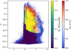 |
Fig. A.1 Example of a 6D completeness mask. This figure represents the ratio of the number of 6D stars and 5D stars (N6D/N5D as a function of apparent colour and magnitude for healpixel number 8 (P6D P6Dmask#8). Yellow colours denote regions where all 5D stars have a radial velocity measurement, whereas dark blue is linked to an absence of radial velocity measurements. We show how, in areas in the CMD not covered by stars from this region, we use the P6D all sky. This is shown in this plot as background, where blue colours denote zero probability and red means 100% probability. |
In a second step, we characterise a new set of parameters that will be crucial to mimic observational effects (we decided to restrict it to a radius of 1.3 kpc around the Sun) in the synthetic CMDs, and that are a function of the apparent magnitudes of the stars: set2 = [parallax_over_error, radial_velocity_error, Δ mG, Δ mbp, Δ mrp], where Δ mG, Δ mbp, and Δ mrp denote the symmetrised photometric errors in the G, Gbp, and Grp apparent magnitudes, respectively. In this second step, and to make sure that the expected (realistic) behaviour prevails (i.e. faint stars are affected by larger uncertainties than brighter stars), we do not assign a random value following the global distribution but stick to specific procedures. For parallax_over_error and radial_velocity_error we characterise the observed distribution (from the sample we are analysing) of values of both parameters as a function of apparent colour and magnitude from the full observed dataset, and assign to each synthetic star a value according to its position in the apparent CMD. Those simulated values will be randomly generated from a Gaussian distribution centred at the average value of the full sample at that apparent colour and magnitude, using a σGauss that is equal to the dispersion of observed values in said position. In the case of the uncertainties in the photometric magnitudes we use a linear fit of the run of observed error in the apparent magnitude with respect to such magnitude (i.e. Δ mx versus mx with x being G, Gbp, and Grp; see Riello et al. 2021; Fabricius et al. 2021).
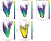 |
Fig. A.2 Error and completeness simulation using GAIA-DisPar. Top left panel: Original synthetic CMD, complete and not affected by observational errors. Top middle panel: Synthetic CMD after completeness has been simulated. We note that many stars in the upper main sequence are lost due to the blue sharp cut in the apparent colour of the P6Dmask. Top right panel: Final synthetic CMD, considering both completeness and error simulation. This will be the synthetic CMD used in the computation of the SFH using DirSFH. Bottom left panel: Ratio of the synthetic CMD after completeness and the original one. We note the clear effect on the distribution of stars in the CMD due to the RVS sample selection. Bottom right panel: Ratio of the original synthetic CMD and the dispersed one to highlight the widening of some areas, especially at fainter magnitudes. |
In a third step, we refine all these parameters (set1 and set2), by finding counterparts of the synthetic stars in the observed CMD of the full sample. If a given synthetic star has 10 or more observed stars near its position in the CMD (Euclidean distance below 0.05 mag), then we link this synthetic star to one of the 10 closest observed stars, and assign new values for these parameters based on those of the linked observed stars (modified according to typical uncertainties14). If no counterpart is found, as in the hypothetical case of a synthetic star located in the bright main sequence if the observed sample is drawn from the (old) halo, then the previously simulated values are retained. This approach allows us to simultaneously have a synthetic mother CMD that is faithful to the properties of the particular observed sample (full) and display the typical behaviour of Gaia data uncertainties beyond the particular CMD coverage of the sample under study.
To mimic a hypothetical observation of the stars in the synthetic CMD with the Gaia satellite, we still have to take into account the Gaia selection function. Due to technical limitations of the Gaia observations, we do not have parameters (5D or 6D) for every star in our Galaxy. Cantat-Gaudin et al. (2023) empirically quantified the completeness of the catalogue of Gaia’s third data release (DR3). The authors made their model available through the gaiaunlimited Python package. Given a location in our Galaxy (l, b and distance), as well as the apparent colour (G−Grp) and magnitude (G) of a star, this package provides the probability of such star being part of the 5D (P5D) Gaia catalogue (DR3SelectionFunctionTCG). In the previous steps, we simulated all these observed quantities for every synthetic star, and thus, we could compute the probability of each synthetic star to make it to the 5D catalogue (allowing the simulation of completeness effects in our synthetic CMD). For samples defined using the Gaia 5D sample the probability of synthetic star to belong to the Gaia catalogue is given by P=P5D).
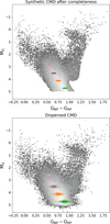 |
Fig. A.3 Error simulation using DisPar-Gaia. Top panel: Synthetic CMD before error simulation. To illustrate observational uncertainties some particular regions are highlighted in different colours. Bottom panel: Same synthetic CMD after simulating photometric errors using GAIA-DisPar. The coloured points represent the position of the synthetic stars highlighted in the top panel after the error simulation. As expected, fainter stars are more affected by observational uncertainties than brighter stars. |
For samples defined based on RVS information (as in this paper), we also need to simulate the probability of a star to belong to the 6D Gaia catalogue (P6D). For this, rather than using the implementation by Cantat-Gaudin et al. (2023), we have decided to use an alternative, empirical approach. First, we assess the volume within which we can compute SFHs based on the RVS sample. Based on the apparent G-band magnitude limit of the RVS sample, and our need to get as faint as the oMSTO, we decided to restrict it to a radius of 1.3 kpc15 around the Sun. Then, given that we are mainly interested in describing how completeness and errors affect the overall distribution of stars in the CMD, we have computed P6D as the ratio of the number of stars with 6D and 5D information (N6D/N5D) in small cells across the apparent CMD (see Fig. A.1, we call this P6Dmask16). Given that the 6D completeness slightly depends on position in the sky, but also considering that for our method we need a large number of stars to properly estimate P6D with enough colour and magnitude resolution, we characterise such ratio using 12 different P6Dmasks by dividing the sky in 12 different healpixels (nside = 1) and an all-sky one. Each mask will contain the corresponding P6D of a given region of the sky across the apparent CMD. This way, for each synthetic star, we can associate its position in the sky with one of the masks, and assign a value of P6D based on its colour and magnitude. In the event that a synthetic star occupies a region in the CMD in which we do not have information, we use the overall mask mentioned before (P6D all sky in Fig. A.1). Once we have assigned to each synthetic star its P5D and-or P6D, we can compute its total probability of being observed by Gaia as P = P5D (in the 5D case) or P=P5D × P6D (in the case of a 6D sample). Finally, we give to each synthetic star a random value ranging from 0 to 1(P*), if P<P*, then such synthetic star is kept, otherwise, we remove it mimicking the Gaia (5D and-or 6D) selection functions.
Finally, completeness is also affected by the quality cuts that transform our full observed sample into the QSHAG observed sample actually used for the fit. We need to simulate these cuts in our synthetic CMD as well. For the cuts that are generally applied -and in particular that have been applied in this work- all parameters involved have been simulated in the synthetic CMD. Thus, we can simply apply the same cuts as in the observed samples (see Sect. 2 in the case of this paper), to automatically take into account the incompleteness derived from such quality cuts in our synthetic CMD.
Finally, for the synthetic stars that remain we alter their absolute magnitudes (Mx with x being G, Gbp, and Grp) in order to simulate the observational errors. For this, we analysed the following equation to compute absolute magnitudes in a given filter x(Mx):
 (A.1)
where mx is the apparent magnitude in MG, Gbp, or Grp, Ax the extinction, and parallax its parallax in mas units17. By applying the corresponding derivatives (error propagation), the total error is given by
(A.1)
where mx is the apparent magnitude in MG, Gbp, or Grp, Ax the extinction, and parallax its parallax in mas units17. By applying the corresponding derivatives (error propagation), the total error is given by
 (A.2)
where Δmx correspond to the photometric uncertainties in the apparent magnitudes, ΔAx is the error in the extinction coefficient (including intrinsic error of the dust map, as well as the one derived from the uncertainty in the position or distance), and Δ MX, dist is the error due to the uncertainty in the distance determination, which is computed as
(A.2)
where Δmx correspond to the photometric uncertainties in the apparent magnitudes, ΔAx is the error in the extinction coefficient (including intrinsic error of the dust map, as well as the one derived from the uncertainty in the position or distance), and Δ MX, dist is the error due to the uncertainty in the distance determination, which is computed as
 (A.3)
(A.3)
Finally, we modify the absolute magnitude in each Gaia passband based on this determination of the uncertainty in the absolute magnitudes. In this way, the modified magnitude (M’x) in each filter will be given by
 (A.4)
where σMx is a correction generated randomly from a Gaussian distribution centred at Mx and with a σgauss of ΔMx (see Equation A.2). The final outcome of applying DisPar-Gaia to a synthetic CMD mimicking Gaia observational effects for a sample defined in 6D (RVS) is shown in Figs. A.2 and A.3. Such synthetic CMD, including errors and completeness effects, can be directly compared to our observed QSHAG sample in order to compute SFHs using DirSFH. Along this and other works, we call this new synthetic mother CMD the “dispersed” mother CMD.
(A.4)
where σMx is a correction generated randomly from a Gaussian distribution centred at Mx and with a σgauss of ΔMx (see Equation A.2). The final outcome of applying DisPar-Gaia to a synthetic CMD mimicking Gaia observational effects for a sample defined in 6D (RVS) is shown in Figs. A.2 and A.3. Such synthetic CMD, including errors and completeness effects, can be directly compared to our observed QSHAG sample in order to compute SFHs using DirSFH. Along this and other works, we call this new synthetic mother CMD the “dispersed” mother CMD.
Appendix B The mask
The comparison between spectroscopic measurements and our resulting metallicity distributions must account for the fact that spectroscopic observations are inherently less numerous and more incomplete than photometric observations. This discrepancy arises because the selection functions of spectroscopic surveys are limited to specific targets in the sky, whereas Gaia’s photometric observations encompass all stars up to a magnitude G ∼ 21.
To address this issue, we compute a mask that ensures consistency between the datasets. This mask is created by computing the fraction of stars observed spectroscopically with respect to the Gaia photometric observations in bins of colour and magnitude, i.e. Nspec/Nphot. The bins are square regions with sides of 0.1 magnitudes. Then, within our solution CMD we randomly select the corresponding fraction of stars in the same bins of colour and magnitude.
Figure B.1 shows an example of the mask computed for APOGEE observations in our volume which verifies the ks_thin disc selection. The upper and middle panels show the density of stars with spectroscopic and photometric observations, respectively, across the CMD. The bottom panel shows the division of the two, that is, the fraction of stars observed spectroscopically with respect to the photometric observations in each bin of colour and magnitude.
Figure B.2 displays on the left panel the best-fit solution of the ks_thin disc. The right panel shows the distribution in the CMD of the solution after applying the mask computed following the APOGEE spectroscopic observations in our volume. These stars from the masked solution are the ones whose metallicities would be compared with APOGEE spectroscopic data in Section 3.2. The same method is computed for comparisons with the other spectroscopic surveys analysed in Sections 3.2 and 3.3.
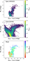 |
Fig. B.1 Top panel: Density map in the colour-magnitude diagram, in bins of 0.1 mag in MG and GBP-GRP of APOGEE spectroscopic observations within the volume analysed. Middle panel: Same as top panel by for Gaia photometric observations in the volume analysed. Bottom panel: Mask, that is the fraction of spectroscopic measurements with respect to the photometric observations in the same bins as top and middle panels. |
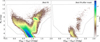 |
Fig. B.2 Left panel: Density map of the best-fit solution for the ks_thin disc selection. Right panel: Density map of the best-fit solution after applying the mask computed following the APOGEE spectroscopic observations in our cylindrical local volume. |
Appendix C Testing probabilities
In this appendix, we test how selection based on probability impacts the resulting deSFHs and explore what this reveals about the kinematic transition from hotter to cooler orbits over time.
Figure C.1 presents the deSFH obtained from stars with a probability higher than 90% of belonging to the ks_thick (top) and ks_thin (bottom) discs. The deSFHs closely resemble those derived from stars with probabilities higher than 75%, particularly for the ks_thick disc. However, the younger episode of star formation with super-solar metallicities is weaker in this case. For the ks_thin disc, the deSFH of stars with probabilities exceeding 90% is more concentrated at ages around ∼ 3 Gyr and younger than 1 Gyr. Nonetheless, all the features identified in the deSFH of stars with probabilities greater than 75%, as discussed in the main text, are also present here.
Figure C.2 shows the deSFH of stars with probabilities lower than 75% of belonging to the ks_thick (top) and ks_thin (bottom) discs (and higher than 50% since they have been classified as belonging to these components). For the ks_thick disc, we exclude the stars with probabilities higher than 25% of belonging to the ks_halo. It is worth noting that stars with probabilities lower than 75% constitute a minority of the total population in the ks_thick and ks_thin discs. They do not contribute significantly to the total deSFH, as Figure C.3 demonstrates. These stars exhibit kinematics between those of the final selection for ks_thin and ks_thick disc stars, as illustrated in Figure C.4.
The deSFH indicates that ks_thick disc stars with cooler orbits align the younger and more metal-rich end of the hotter ks_thick disc deSFH, preserving the distinction between the two episodes of star formation below and above solar metallicity. The ks_thin disc with probabilities lower than 75% concentrates at older ages (between 11 and 6) than the cooler ks_thin disc, with only a few younger and less prominent star formation events occurring at later ages, and very few stars younger than 3 Gyr. This corroborates that we are seen a transition in age and metallicity with the kinematic cooling of the Milky Way disc. This analysis underscores the kinematic settlement that the Milky Way experienced over a relatively short period of time.
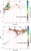 |
Fig. C.1 Dynamically evolved star formation rates as a function of age and metallicity, as in Figure 4. In this case only stars with probability higher than 90% of belonging to the ks_thick (top) and ks_thin (bottom) discs have been analysed. |
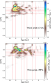 |
Fig. C.2 Dynamically evolved star formation rates as a function of age and metallicities as in Figure 4. In this case, only stars with probabilities between 50% and 75% of belonging to the ks_thick (top) and ks_thin (bottom) discs have been analysed. |
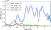 |
Fig. C.3 Dynamically evolved star formation rates as a function of stellar age derived for the ks_thick (blue), ks_thin (red) discs, and for the stars with probabilities between 50% and 75% of belonging to the kinematic thick disc (orange) and kinematic thin disc (green). |
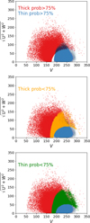 |
Fig. C.4 Top panel: Toomre diagram of the selected ks_thin disc (blue) and ks_thick disc (red) stellar samples, considering quality selection criteria, as in Figure 2. Middle panel: Same as the top panel but with stars with probabilities between 50% and 75% of belonging to the kinematic thick disc over plotted in orange. Bottom panel: Same as top panel but with stars with probabilities between 50% and 75% of belonging to the kinematic thin disc overplotted in green. |
All Figures
|
Fig. 1 Top panels: probability of stars of belonging to the ks_thick (red), ks_thin (blue) disc, or ks_halo as a function of fraction of stars (left) and a zoom-in of a small fraction of stars to help visualise the halo probabilities (right). Middle panels: velocity components U (left), V (middle), and W (right) distributions of selected ks_thick (red) and ks_thin (blue). Bottom panels: distribution of the heliocentric radius projection over the Galactic plane, R, (left), and distance from the plane, z, (right) of the selected ks_thick (red) and ks_thin (blue). |
| In the text | |
|
Fig. 2 Toomre diagram of the selected ks_thin disc (blue), ks_thick disc (red), and halo (grey) stellar samples considering the quality selection criteria. |
| In the text | |
|
Fig. 3 Observed (left) and best-fit solution (middle) CMDs and the residuals (right) for the ks_thick disc (top) and ks_thin disc (bottom). The region used in the fit is plotted enclosed by a black polygon. |
| In the text | |
|
Fig. 4 Top panels: dynamically evolved star formation histories, i.e., the stellar mass formed as a function of age and total metallicity ([Z/H]), for the ks_thick (left) and ks_thin (right) discs. Middle panels: same as top panels but including contour lines indicating the signal-to-noise ratio (S/N) of the resulting deSFH. Bottom panels: age and metallicity distribution of living stars in the volume analysed. The colour code indicates now the number of stars per bin in a 100 × 100 grid. In top and bottom panels: red dotted lines mark key age and metallicity values (11, 10, 8, 7, 6, 4 and 3 Gyr) and metallicity values (from 0 to −0.4 in steps of 0.1 dex). The contour lines enclose the 10%, 25%, 50%, 75%, and 95% of M⊙ Gyr−1 dex−1 (top) and the number of stars (bottom) within the age range of 13.5 to 8 Gyr and metallicity range of [Z/H] between −2 and −0.4, highlighting the structure within this region of parameter space. |
| In the text | |
|
Fig. 5 Dynamically evolved star formation rate as a function of stellar age derived with CMDft.Gaia for the ks_thick (red) and ks_thin (blue) discs. Shaded area around each curve represents one standard deviation. |
| In the text | |
|
Fig. 6 Metallicity distribution functions for the ks_thick disc (top panels) and the ks_thin disc (bottom panels) derived from our solution CMDs compared with those obtained from the spectroscopic surveys APOGEE (left), GALAH (middle), and the Golden Sample of Gaia-RVS (right). The red or blue curves correspond to the spectroscopic MDFs, and the black lines display the MDF distribution from each corresponding masked solution CMD (see text for details). |
| In the text | |
|
Fig. 7 Left panels: age-metallicity distribution of the masked solutions for ks_thick disc stars (top, represented by individual red points) and ks_thin disc stars (bottom, shown as a blue-scale hexbin density diagram). This is the same solution as Figure 4 bottom panels, i.e., the distribution of synthetic stars from the best fit which corresponds to the age-metallicity distributions of the living stars in the volume analysed. Right panels: [Mg/Fe] versus [Z/H] (global metallicity; see Section 3.2 in the main text) based on spectroscopic measurements from APOGEE DR17 and GALAH DR3, homogenised using the SpectroTranslator. The ks_thick disc stars are displayed at the top (with individual red points), while ks_thin disc stars appear at the bottom (as a blue-scale hexbin density diagram). The isocontours in red (blue) display the 30%, 60%, and 90% percent of the stellar distribution in the chemical space corresponding to the ks_thin disc(ks_thick disc) in addition to the ks_thick disc(ks_thin disc) stars. The vertical black dashed lines indicate the metallicity ranges of interest discussed in the main text. |
| In the text | |
|
Fig. A.1 Example of a 6D completeness mask. This figure represents the ratio of the number of 6D stars and 5D stars (N6D/N5D as a function of apparent colour and magnitude for healpixel number 8 (P6D P6Dmask#8). Yellow colours denote regions where all 5D stars have a radial velocity measurement, whereas dark blue is linked to an absence of radial velocity measurements. We show how, in areas in the CMD not covered by stars from this region, we use the P6D all sky. This is shown in this plot as background, where blue colours denote zero probability and red means 100% probability. |
| In the text | |
|
Fig. A.2 Error and completeness simulation using GAIA-DisPar. Top left panel: Original synthetic CMD, complete and not affected by observational errors. Top middle panel: Synthetic CMD after completeness has been simulated. We note that many stars in the upper main sequence are lost due to the blue sharp cut in the apparent colour of the P6Dmask. Top right panel: Final synthetic CMD, considering both completeness and error simulation. This will be the synthetic CMD used in the computation of the SFH using DirSFH. Bottom left panel: Ratio of the synthetic CMD after completeness and the original one. We note the clear effect on the distribution of stars in the CMD due to the RVS sample selection. Bottom right panel: Ratio of the original synthetic CMD and the dispersed one to highlight the widening of some areas, especially at fainter magnitudes. |
| In the text | |
|
Fig. A.3 Error simulation using DisPar-Gaia. Top panel: Synthetic CMD before error simulation. To illustrate observational uncertainties some particular regions are highlighted in different colours. Bottom panel: Same synthetic CMD after simulating photometric errors using GAIA-DisPar. The coloured points represent the position of the synthetic stars highlighted in the top panel after the error simulation. As expected, fainter stars are more affected by observational uncertainties than brighter stars. |
| In the text | |
|
Fig. B.1 Top panel: Density map in the colour-magnitude diagram, in bins of 0.1 mag in MG and GBP-GRP of APOGEE spectroscopic observations within the volume analysed. Middle panel: Same as top panel by for Gaia photometric observations in the volume analysed. Bottom panel: Mask, that is the fraction of spectroscopic measurements with respect to the photometric observations in the same bins as top and middle panels. |
| In the text | |
|
Fig. B.2 Left panel: Density map of the best-fit solution for the ks_thin disc selection. Right panel: Density map of the best-fit solution after applying the mask computed following the APOGEE spectroscopic observations in our cylindrical local volume. |
| In the text | |
|
Fig. C.1 Dynamically evolved star formation rates as a function of age and metallicity, as in Figure 4. In this case only stars with probability higher than 90% of belonging to the ks_thick (top) and ks_thin (bottom) discs have been analysed. |
| In the text | |
|
Fig. C.2 Dynamically evolved star formation rates as a function of age and metallicities as in Figure 4. In this case, only stars with probabilities between 50% and 75% of belonging to the ks_thick (top) and ks_thin (bottom) discs have been analysed. |
| In the text | |
|
Fig. C.3 Dynamically evolved star formation rates as a function of stellar age derived for the ks_thick (blue), ks_thin (red) discs, and for the stars with probabilities between 50% and 75% of belonging to the kinematic thick disc (orange) and kinematic thin disc (green). |
| In the text | |
|
Fig. C.4 Top panel: Toomre diagram of the selected ks_thin disc (blue) and ks_thick disc (red) stellar samples, considering quality selection criteria, as in Figure 2. Middle panel: Same as the top panel but with stars with probabilities between 50% and 75% of belonging to the kinematic thick disc over plotted in orange. Bottom panel: Same as top panel but with stars with probabilities between 50% and 75% of belonging to the kinematic thin disc overplotted in green. |
| In the text | |
Current usage metrics show cumulative count of Article Views (full-text article views including HTML views, PDF and ePub downloads, according to the available data) and Abstracts Views on Vision4Press platform.
Data correspond to usage on the plateform after 2015. The current usage metrics is available 48-96 hours after online publication and is updated daily on week days.
Initial download of the metrics may take a while.