| Issue |
A&A
Volume 704, December 2025
|
|
|---|---|---|
| Article Number | A346 | |
| Number of page(s) | 17 | |
| Section | Cosmology (including clusters of galaxies) | |
| DOI | https://doi.org/10.1051/0004-6361/202554045 | |
| Published online | 22 December 2025 | |
The SRG/eROSITA All-Sky Survey
Constraints on ultralight axion dark matter through galaxy cluster number counts
1
Max Planck Institute for Extraterrestrial Physics, Giessenbachstrasse 1, 85748 Garching, Germany
2
Universität Innsbruck, Institut für Astro- und Teilchenphysik, Technikerstr. 25/8, 6020 Innsbruck, Austria
3
INAF, Osservatorio di Astrofisica e Scienza dello Spazio, Via Piero Gobetti 93/3, I-40129 Bologna, Italy
4
Department of Physics and Astronomy, Stony Brook University, Stony Brook, NY 11794, USA
5
Universität Hamburg, Hamburger Sternwarte, Gojenbergsweg 112, 21029 Hamburg, Germany
6
Department of Physics, National Cheng Kung University, 70101 Tainan, Taiwan
7
IRAP, Université de Toulouse, CNRS, UPS, CNES, F-31028 Toulouse, France
8
University of Cambridge, Cavendish Laboratory and DAMTP, Cambridge CB3 0WA, United Kingdom
9
Kobayashi-Maskawa Institute for the Origin of Particles and the Universe (KMI), Nagoya University, Nagoya 464-8602, Japan
10
Institute for Advanced Research, Nagoya University, Nagoya 464-8601, Japan
11
Kavli Institute for the Physics and Mathematics of the Universe (WPI), The University of Tokyo Institutes for Advanced Study (UTIAS), The University of Tokyo, Chiba 277-8583, Japan
12
Subaru Telescope, National Astronomical Observatory of Japan, 650 N Aohoku Place, Hilo, HI 96720, USA
13
Department of Physical Science, Hiroshima University, 1-3-1 Kagamiyama, Higashi-Hiroshima, Hiroshima 739-8526, Japan
14
Department of Astronomy, University of Geneva, Ch. d’Ecogia 16, CH-1290 Versoix, Switzerland
15
Universitäts-Sternwarte, Faculty of Physics, LMU Munich, Scheinerstr. 1, 81679 München, Germany
★ Corresponding author: This email address is being protected from spambots. You need JavaScript enabled to view it.
Received:
5
February
2025
Accepted:
5
October
2025
Abstract
Ultralight axions are hypothetical scalar particles that influence the evolution of large-scale structures of the Universe. Depending on their mass, they can potentially be part of the dark matter component of the Universe as candidates commonly referred to as fuzzy dark matter. While strong constraints have been established for pure fuzzy dark matter models, the more general scenario where ultralight axions constitute only a fraction of the dark matter has been limited to only a few observational probes. In this work, we use the galaxy cluster number counts obtained from the first All-Sky Survey (eRASS1) of the SRG/eROSITA mission together with gravitational weak lensing data from the Dark Energy Survey, the Kilo-Degree Survey, and the Hyper Suprime-Cam to constrain the fraction of ultralight axions in the mass range 10−32 eV to 10−24 eV. We put upper bounds on the ultralight axion relic density Ωa in independent logarithmic axion mass bins by performing a full cosmological parameter inference. We find an exclusion region in the intermediate ultralight axion mass regime with the tightest bounds reported so far in the mass bins around ma = 10−27 eV with Ωa < 0.0035 and ma = 10−26 eV with Ωa < 0.0079; both are at a 95% confidence level. When combined with cosmic microwave background probes, these bounds are tightened to Ωa < 0.0030 in the ma = 10−27 eV mass bin and Ωa < 0.0058 in the ma = 10−26 eV mass bin, with both at a 95% confidence level. This is the first time that constraints on ultralight axions have been obtained using the growth of structure measured by galaxy cluster number counts. These results pave the way for large surveys, which can be utilized to obtain tight constraints on the mass and relic density of ultralight axions with better theoretical modeling of the abundance of halos.
Key words: galaxies: clusters: general / galaxies: clusters: intracluster medium / cosmological parameters / cosmology: observations / dark matter / large-scale structure of Universe
© The Authors 2025
 Open Access article, published by EDP Sciences, under the terms of the Creative Commons Attribution License (https://creativecommons.org/licenses/by/4.0), which permits unrestricted use, distribution, and reproduction in any medium, provided the original work is properly cited.
This article is published in open access under the Subscribe to Open model. This email address is being protected from spambots. You need JavaScript enabled to view it. to support open access publication.
1. Introduction
According to the Lambda cold dark matter (ΛCDM) paradigm, the Universe is composed of two species of matter: baryonic matter and cold dark matter. The latter’s potential interactions with the fundamental constituents of the standard model of particle physics are below the sensitivity of modern experiments, in particular its couplings with photons. Additionally, the ΛCDM includes a dark energy component responsible for the accelerated expansion of the Universe, which is parameterized by the cosmological constant Λ. Various cosmological probes have provided tight constraints on the dark matter, baryonic matter, and dark energy content of the Universe, for example, through the analysis of the cosmic microwave background (CMB) (Planck Collaboration XXIV 2016; Planck Collaboration VI 2020; Hinshaw et al. 2013), Type Ia supernovae (Abbott et al. 2019; DES Collaboration 2024; Scolnic et al. 2022; Brout et al. 2022), cluster abundance (Ghirardini et al. 2024, G24 hereafter, Bocquet et al. 2024, Costanzi et al. 2021, Lesci et al. 2022), weak lensing shear (Asgari et al. 2021; Abbott et al. 2022; Amon et al. 2022; Miyatake et al. 2023; Dalal et al. 2023), and galaxy clustering (Zhao et al. 2022; Adame et al. 2025).
Despite the constraints on the density of dark energy and dark matter obtained by state-of-the-art cosmological studies, their nature remains elusive. Consequently, potential extensions of ΛCDM with viable dark matter candidates have been explored using observations of the large-scale structure, such as axion-like particles (ALPs), and self-interacting dark matter (Randall et al. 2008; Conlon et al. 2017). The ALPs are promising potential dark matter candidates. Depending on their properties, ALPs can also partially explain dark energy. ALPs are scalar fields with typically tiny masses, compared to known elementary particles, that move in a periodic potential. Historically, the so-called quantum chromodynamics (QCD) axion was proposed by Peccei & Quinn (1977a,b) to solve a fine-tuning problem of QCD, known as the strong charge parity (CP) problem. Although predicted by QCD, the strong CP problem refers to unobserved violations of simultaneous charge conjugation (C) and parity (P). Particles with the same underlying physics naturally occur in string theory due to the compactification of large extra dimensions and are called axions or ALPs (Svrcek & Witten 2006). The typical particle masses can span the range from 10−33 eV to 10−5 eV. In principle, multiple ALPs with a large spectrum of mass might exist in string theory, called the axiverse (Arvanitaki et al. 2010a). Upper bounds on the number of ALP species have been found by superradiance effects of stellar and supermassive black holes (Stott & Marsh 2018) and supernovae (Gendler et al. 2024). ALPs with masses ma ≳ 10−22 eV are candidates to compose a large fraction of dark matter, while ALPs with masses ma ≲ 10−33 eV represent candidates for dark energy.
In the dark energy scenario (ma ∼ 10−33 eV), the axion field exhibits slow-roll behavior due to the small mass of ALPs. As it is still rolling today, the axion field has not yet started to oscillate around the minimum of its potential. Thus, it behaves similarly to a fluid with negative pressure, which is similar to dark energy (Hložek et al. 2015, 2018; Passaglia & Hu 2022). For masses ma ≲ 10−33 eV, the axion field is frozen in, and only its potential energy contributes to the vacuum energy of the Universe. This scenario is indistinguishable from the ΛCDM dark energy with the equation of state w = −1.
In the case of small masses around 10−24 eV, the bosonic nature and negligible self-couplings of ALPs enable them to form Bose-Einstein condensates (BECs) on scales determined by their thermal de Broglie wavelength. The simulations by Schive et al. (2014a) have demonstrated the formation of core-like structures in the center of halos, whose size could be used to obtain constraints on the ALP mass from dwarf galaxies. Over the past decades, a number of simulations of ALPs as dark matter candidates (also called wave-like dark matter) have been performed with increasing resolution and while assuming a cosmology with a dark matter sector fully comprised by ALPs (e.g., Mocz et al. 2018; Nori & Baldi 2018; May & Springel 2021, 2023). With an increasing precision of ALP mass constraints, mixed ALP-cold dark matter simulations became relevant since they can be used to constrain the fraction of ALPs in the Universe (Schwabe et al. 2020; Laguë et al. 2024; Dome et al. 2025). In this axion mass regime, the thermal de Broglie wavelength extends to the cosmological scales, i.e., several kilo- or megaparsecons, making the axion condensates observable in studies of the matter power spectrum. A BEC on these scales forms large core-like structures, smooths out the dark matter distribution, and suppresses the formation of small-scale halos. ALPs have been proposed as a potential solution to the small-scale crisis in cosmology, particularly for addressing discrepancies in structure formation at galactic and subgalactic scales. However, the existence of the small-scale crisis itself has been questioned, with alternative explanations suggesting that baryonic physics or observational limitations may account for the perceived discrepancies (Nori & Baldi 2018; Bullock & Boylan-Kolchin 2017; De Laurentis & Salucci 2022). We refer to these cosmologically interesting low-mass axions with masses ma ≲ 10−24 eV as ultralight axions (ULAs). In the literature, the resulting dark matter is referred to as fuzzy dark matter due to its smoothing effect (e.g., Hu et al. 2000; Hui et al. 2017).
Constraining the coupling constant between ALPs and photons is also feasible, but it requires direct X-ray observations of the intracluster medium (ICM), which have the potential to detect a possible interaction between axions and photons. Such an interaction is only possible in magnetic fields since the axion coupling term is proportional to the scalar product of electric and magnetic fields. Measurements of spectral features in galaxy clusters have been used to constrain the properties of dark matter candidates such as ALPs and decaying dark matter (Bulbul et al. 2014; Conlon et al. 2017; Reynolds et al. 2020). Unlike the studies performed with the probes of structure growth, these analyses can determine bounds on the axion-photon coupling constant and mixing angles, but they cannot constrain the relic density of dark matter candidates.
The viable mass ranges for ULAs and abundances constituting dark matter and dark energy can be constrained through observations of the large-scale structure as well as the CMB and subgalactic scales. In the dark matter regime, where the ULAs make up all of the dark matter by assumption, strong bounds on the ULA parameter space have been reported in the literature. Lyman-alpha forest observations place a lower-mass bound of 2 × 10⁻²⁰ eV, at a 95% confidence level (Rogers & Peiris 2021). The observations of ultrafaint dwarf galaxies tighten this bound to 3 × 10⁻¹⁹ eV, at a 99% confidence level (Dalal & Kravtsov 2022), while superradiance by supermassive black holes can be used to exclude a window of masses around 7 × 10⁻²⁰ eV (Arvanitaki et al. 2015; Cardoso et al. 2018; Stott & Marsh 2018; Stott 2020; Hoof et al. 2025).
The possibility that ULAs may comprise only a fraction of the total abundance of dark matter nevertheless remains. For the first time, CMB data from the Planck satellite (Planck Collaboration XIII 2016) provided strong bounds in the mass regime 10−32 eV to 10−25 eV by performing a binned analysis in different ULA mass bins. They found varying upper bounds on the ULA abundance, reaching down to Ωa ≲ 0.01 in the intermediate mass range of 10−30 − 10−27 eV (Hložek et al. 2015, 2018). The same mass regime has also been constrained by Laguë et al. (2022) and Rogers et al. (2023) using Planck 2018 (Planck Collaboration VI 2020) and Baryon Oscillation Spectroscopic Survey (BOSS; (Alam et al. 2017)) data, improving existing constraints. Kobayashi et al. (2017) used the Lyman-α forest to place bounds on the fraction of ULAs in the higher-mass regime of 10−23 eV to 10−20 eV, and Winch et al. (2024) closed the gap by using UV-bright galaxy abundance to put an upper bound on the ULA fraction in the mass regime 10−26 eV to 10−23 eV. They find that ULAs cannot make up more than 22% of all dark matter in this mass range.
In this work, we use for the first time the observed abundance of galaxy clusters to constrain the parameter space of ULAs. Since the formation of halos is influenced by bosonic condensation, we expect cluster counts to be sensitive to ULAs (Diehl & Weller 2021). We particularly focus on the mass regime 10−32 eV to 10−24 eV. Clusters of galaxies trace the highest peaks in the low-redshift matter density field through their number counts and therefore serve as an important late-time probe of the structure formation in the Universe. Measurements of their number count as a function of mass and redshift bin per unit volume, the so-called cluster halo mass function (HMF), is a sensitive probe of cosmology. The cluster mass function can constrain the ULA mass and abundance parameter space since the growth of structure and bosonic condensation influence the formation of halos.
To this end, we used the clusters of galaxies detected by the extended ROentgen Survey with an Imaging Telescope Array (eROSITA) on board the Spektr-RG (SRG) mission (Sunyaev et al. 2021) during its first All-Sky Survey in the western Galactic hemisphere (eRASS1). eROSITA, launched in 2019, scans the sky in the soft X-ray band with its highest sensitivity in the 0.2 to 2.3 keV energy band (Predehl et al. 2021). eRASS1 provides different cluster catalogs depending on purity and completeness requirements. The primary eRASS1 catalog comprises 12 247 galaxy clusters, with a sample purity of 86% and a coverage of 12 791 deg2 (Bulbul et al. 2024; Kluge et al. 2024). In this work, we use the cosmology sample containing 5 259 securely detected clusters in the redshift range of 0.1 ≤ z ≤ 0.8, which have a sample purity of 96%. The eRASS1 cosmological sample has provided competitive results for standard cosmologies (see G24 for the details of the analysis) as well as modified gravity (Artis et al. 2024) and the growth of structures (Artis et al. 2025). The eRASS1 cosmology sample is the largest ICM-selected galaxy cluster sample ever used to infer cosmology from number counts. The covered cluster mass range extends down into the galaxy group regime, opening the possibility of probing cosmological models sensitive to below-cluster scales. The presence of ULAs has the strongest imprint on the number density of low-mass halos, making the eRASS1 cosmology sample a promising tool to constrain the properties of ULAs. In contrast to the main cosmological inference G24, in this work, to constrain the ULA parameter space, we used the Boltzmann solver axionCAMB instead of CAMB to compute a matter power spectrum that is sensitive to two ULA parameters, particularly the mass of the ULA, ma, and the energy density fraction of ULAs, Ωa, in units of the critical density of the Universe.
This paper is organized as follows. A more detailed overview of the ULAs and their effect on cosmology is given in Sect. 2, including their influence on structure formation. The underlying cosmological sample of the eRASS1 survey and the optical and weak lensing data used for the analysis are summarized in Sect. 3. Section 4 reviews the eRASS1 cluster cosmological pipeline for Bayesian inference in light of the ULA parameters. The results are presented and discussed in Sects. 5 and 6. For better readability, we use natural units c ≡ ℏ ≡ 1 throughout this work.
2. Ultralight axion cosmology
In this section, we first provide a review of the motivation for ULAs as dark matter candidates. We then explain the implications of their existence on the hierarchical structure formation and cosmology.
2.1. Physical origin of axions
Axions are hypothetical pseudoscalar particles with typically low mass (between 10−33 eV and 10−5 eV) and weak couplings to the Standard Model particles (i.e., quadratic coupling terms can be neglected). Pseudoscalar hereby refers to the property that the particle behaves like a scalar under transformations, except parity transformations, under which it switches signs. Although the axion was originally introduced in QCD to solve the strong CP problem explicitly, the term has been extended to a number of (pseudo) Nambu-Goldstone bosons. Nambu-Goldstone bosons are particles that occur as massless degrees of freedom after breaking a spontaneous symmetry. Axions are pseudo-Nambu-Goldstone bosons as they acquire a very small mass via further symmetry breaking. These particles appear in various theories of high energy physics such as string theory (e.g., Svrcek & Witten 2006; Conlon 2006; Arvanitaki et al. 2010b) or supersymmetric extensions of the Standard Model (e.g., Kim & Carosi 2010; Marsh 2016, for review). To distinguish such general axions from the QCD axion, they are often referred to as ALPs or ultralight axions in the cosmologically relevant low-mass regime. The common properties of these particles are well described in Section 2.2 in Marsh (2016).
We heuristically illustrate axion physics using the QCD axion introduced by Peccei & Quinn (1977a,b) as a generic example. We refer the reader to Marsh (2016) for further details. A non-Abelian SU(3) gauge theory with a gluon gauge field  naturally exhibits a topological term with some coupling θ in its Lagrangian density, which is of the form
 (1)
(1)
where  is the dual of the gluon gauge field tensor, μ and ν refer to spacetime coordinates and a is some color index. This term is CP-violating and cannot be transformed away. If QCD is CP-violating, it leads to a non-vanishing neutron electric dipole moment dn ≈ θ (3.6 × 10⁻¹⁶e cm) (Crewther et al. 1979). However, experiments place strong constraints on the neutron electric dipole moment (Abel et al. 2020), which results in a fine-tuned value of θ ≲ 10−10. In other words, QCD appears to be non-CP-violating, although it should. This is known as the strong CP problem.
Peccei & Quinn (1977a,b) solved this problem by generalizing the coupling constant θ to a scalar field that naturally cancels any contribution to the CP-violating term. To this end, they introduced a new global UPQ(1) symmetry, known as the Peccei-Quinn symmetry. The spontaneous breaking of this symmetry at a high energy scale fa leads to a vacuum manifold that is isomorphic to the one-sphere S1. The emerging Nambu-Goldstone boson (which will become the axion later) is an angular degree of freedom in an effectively flat potential. Thus, at this point, the new particle is massless. At some lower energy scale, Λa (not to be confused with the cosmological constant Λ), non-perturbative QCD effects (e.g., instantons, topological effects) break the flatness of the vacuum manifold, the massless Nambu-Goldstone boson lives in. Due to the angular nature of the Nambu-Goldstone boson, only a discrete angular shift symmetry is preserved. Ultimately, the Nambu-Goldstone boson acquires a mass and is canonically called an axion. Simplifying further, the field rolls into the circular minimum of a sombrero-like potential during the first spontaneous symmetry breaking. The Nambu-Goldstone boson is the angular degree of freedom that moves freely along the minimum of the potential. The angular shift symmetry of this potential is then broken by nonperturbative effects, leading to local minima and maxima along the former circular minimum of the potential. Particles moving in a potential with minima acquire a mass; thus, the Nambu-Goldstone boson becomes a massive axion particle.
The axion mass is related to the symmetry-breaking scales fa and Λa. A typical but not unique effective axion potential can take the form
![Mathematical equation: $$ \begin{aligned} V(\phi ) = \Lambda _{\rm a}^4 \left[ 1-\cos \left( \frac{\phi }{f_{\rm a}} \right) \right]. \end{aligned} $$](/articles/aa/full_html/2025/12/aa54045-25/aa54045-25-eq4.gif) (2)
(2)
Considering small oscillations around one of the local minima gives the effective mass of the axion by approximating the local environment of the minimum with a quadratic function:
 (3)
(3)
 (4)
(4)
The mass of the axion can be read off as ma = Λa2/fa. Typical values of fa lie between 109 GeV and 1017 GeV in the QCD case and, in the general case, above 1010 GeV with typical values around the grand unified theory (GUT) scale at 1016 GeV (Marsh 2016). In general, self-interactions are thus suppressed by ma2/fa2 ≲ 10−90 for the ULA mass regime considered in this work, and we make the assumption that self-interactions are negligible in our analysis.
The underlying mechanisms of the QCD axion also apply to axions in string theory models. However, in string theory, the periodicity of the axion potential originates from the compactification of extra dimensions, i.e., extra dimensions are wrapped up, which makes them unobservable by macroscopic observers. The need for extra dimensions in string theory, which have not been observed yet, leads to a natural production mechanism of axion particles with a potentially wide range of possible axion masses.
2.2. Cosmological implications of ultralight axions
This section reviews the implications of an ultralight axion fluid on cosmology. For in-depth discussion and derivations, we refer the reader to the derivations presented in Marsh (2016), Hložek et al. (2015), and Hložek et al. (2018). The ULA field enters the Einstein-Hilbert action of general relativity as a massive scalar field in curved spacetime. On a Friedmann-Lemaître-Robertson-Walker metric background, the Klein-Gordon equation (equation of motion) of the ULA is
 (5)
(5)
Here,  is the Hubble parameter, ϕ is the ULA field, and dots refer to derivatives in time. This equation describes a harmonic oscillator in ϕ with a damping term proportional to the Hubble parameter H. For this illustration, we neglect any source terms from other cosmological fluid components or self-interactions, which would enter the equation on the right-hand side and replace the zero. For H ≪ ma, i.e., if the ULA mass is orders of magnitude larger than the Hubble parameter, the damping term is negligible, and the ULA field oscillates freely. If the ULA’s mass is sufficiently large, this describes the matter-like late-time behavior of the ULA. For the opposite case, H ≫ ma, the field is overdamped and frozen in, showing the same behavior as dark energy. The transition between the two regimes defines a scale aosc which can be approximated by H(aosc)≈ma. In this regime, the ULA is slow-rolling. Thus, a single ULA species may transition from a dark energy-like behavior to a dark matter-like behavior. As the universe evolves in the opposite direction from matter-dominated to dark energy-dominated era, no single ULA species can describe both dark matter and dark energy. We therefore distinguish two distinct phenomenological regimes for ULAs: the dark matter regime, where they behave as dark matter, and the dark energy regime, where they show the same observed effect of dark energy. We review the two regimes in the following subsections.
2.3. Dark matter regime of ultralight axions
Introducing perturbations to the ULA field and choosing a gauge yields an equation for the evolution of perturbations in terms of the ULA overdensity δa = δρa/ρa. In the simple case of a ULA-dominated universe, it takes the form
 (6)
(6)
where k is the wave number, a the scale factor, ρa describes the background density field of the ULA, δρa its perturbation. Other potential fluid components would add source terms to the equation. The effective sound speed of ULAs (cs, a) becomes
 (7)
(7)
Equation (6) defines a scale-dependent Jeans scale kJ for ULAs. As described in Marsh (2016), large-scale perturbations (k < kJ) grow and behave similarly to CDM. Small-scale perturbations (k > kJ) oscillate, making them distinct from CDM perturbations on the same scales. As described in Marsh et al. (2012), modes entering the horizon while the ULA sound speed in Eq. (7) is near the speed of light will suppress structure formation, while modes entering the horizon while the ULA sound speed is approaching zero will cluster like ordinary cold dark matter. Effectively, this translates to suppressing the matter power spectrum on small physical scales (large values of the wave number k).
The properties of ULAs and their cosmological effects can be described with two quantities: The particle mass of the ULA ma, and the relative energy density of ULAs with respect to the critical density of the universe, Ωax = ρax/ρcrit, also known as the relic density of ULAs. Here, the critical density of the universe is defined as ρcrit = 3H02/(8πG). The ΛCDM cosmology is recovered when Ωa → 0. Furthermore, the ULAs’ suppression imprint on the matter power spectrum becomes negligible for high ULA masses ma ≫ 10−22 eV, effectively recovering a ΛCDM cosmology in the context of this analysis. Fig. 1 demonstrates the suppression effect of ULA dark matter with different logarithmic particle masses log10(ma[eV]) and relic densities Ωa on the matter power spectrum. Suppression of the power can be seen on small scales (large k), whereby the effect is stronger with higher ULA fractions or lower ULA masses.
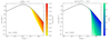 |
Fig. 1. Effect of ULAs on the matter power spectrum recovered assuming the Planck Collaboration VI (2020) cosmological values (ΩΛ ≈ 0.7, Ωm + Ωa ≈ 0.3) at z = 0.1. On the left, the change in the matter power spectrum with varying ULA mass is shown when the relative ULA density is fixed to Ωa/(Ωcdm + Ωa) = 0.5. The panel on the right displays the dependence of the power spectrum on varying ULA abundance at a fixed ULA mass of ma = 10−25 eV. The concordance ΛCDM model is shown in a black curve on both panels. Small-scale suppression becomes stronger with decreasing ULA mass and increasing ULA abundance. For higher ULA masses of ma ≫ 10−22 eV, the matter power spectrum becomes indistinguishable from the one in a ΛCDM cosmology, as is the case for Ωa → 0. |
In this work, we explore whether a fraction of dark matter is composed of ULAs of an unknown mass in the dark matter regime. We still need to postulate a cosmological constant, dark energy, in this context. As we assume a flat universe, the dark energy density is given by ΩΛ = 1 − Ωm − Ωa, while we fit for the total matter density Ωm and the ULA density Ωa. The results are provided in Sect. 5.
2.4. Dark energy regime of ultralight axions
If the ULA is so light that its mass becomes comparable with or smaller than the Hubble parameter H0, the oscillation scale aosc approaches or even exceeds the current scale factor of the universe a(z = 0) = 1, indicating that the ULA field has not started oscillating yet. Indeed, this kind of field behaves as dark-energy-like, which can be heuristically illustrated with the equation of motion. Neglecting the ma2ϕ2 term in Eq. (5) and assuming that H(t) varies slowly enough in time exhibits exponential modes for the ULA field ϕ. This behavior is associated with an equation of state wax ≈ −1 via the density and pressure of the ULA field. In terms of the de Broglie wavelength associated to the ULA BEC, in the extreme case of H0 ≈ ma which occurs around ULA masses of ma ≈ 10−33 eV the de Broglie wavelength is comparable to the size of the universe leading to an overall energy shift, typically associated to a dark energy-like component. However, even at higher ULA masses, as long as the de Broglie wavelength of the ULA BEC exceeds its Jeans scale, ULAs cannot form halos and are thus still referred to as dark energy-like ULAs. Furthermore, if the ULA BEC de Broglie wavelength is comparable to the size of the universe, this affects the Hubble rate and therefore also the distance measurements. This results in a redshift-dependent transition in the Hubble rate, with the nature of the transition dependent on the ULA mass. Wherever the de Broglie wavelength exceeds the size of the universe, ULAs should be modeled as a dark energy component in the Hubble rate. In the opposite case of a de Broglie wavelength smaller than the size of the universe, ULAs should be modeled as a dark matter component in the Hubble rate. The transition between the two regimes is determined by the oscillation redshift. Fig. 2 illustrates the dependence of the oscillation redshift on the ULA mass. We emphasize here that the regime change in the Hubble rate is not related to the typically referenced regime change between dark energy-like ULAs’ and dark matter-like ULAs’ contribution to halo formation, which is determined by the respective Jeans scale.
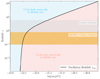 |
Fig. 2. Demonstration of the ULA mass and redshift dependent regime change in the Hubble rate. In the pink regime, ULAs contribute to the Hubble rate e in a manner similar to dark matter; in the blue region, ULAs contribute to the Hubble rate in a dark energy-like fashion. The orange shaded region shows the eRASS1 cluster redshift range, while the gray shaded region shows the redshift range of lensed galaxies from the DES, HSC, and KiDS data, described in Sect. 3.2. Above a ULA mass of ma ∼ 10−31.5 eV, ULAs should be modeled as dark matter in the Hubble rate, resulting in correct distance measurements during the parameter inference. For ULAs with masses below ma ∼ 10−31.5 eV, the distance measurements are affected by the regime change via the Hubble rate, where ULAs are treated as dark energy. |
3. Multiwavelength data
3.1. eROSITA cluster catalog and X-ray observable
This work uses the cosmology sample compiled from the first eROSITA All-Sky Survey (Merloni et al. 2024; Bulbul et al. 2024; Kluge et al. 2024). This sample is constructed by employing an extent likelihood cut of ℒext > 6 and a redshift range of 0.1 ≤ z ≤ 0.8. The publicly available DESI Legacy Survey Data Release 10 (LS DR10) data are used for the confirmation, identification, and photometric redshift measurements of the X-ray-selected cluster candidates detected in the eROSITA All-Sky Survey’s western Galactic hemisphere (Kluge et al. 2024). The common footprint between eRASS1 and the LS DR10-South footprint is 12 791 deg2, and contains 5,259 securely confirmed clusters (Kluge et al. 2024). Its purity level is estimated to be 96%.
The eROSITA X-ray data are reprocessed with the eSASS software as described in Merloni et al. (2024) by applying a correction for the Galactic absorption and a more accurate ICM and background modeling. The details of the X-ray processing are provided in Bulbul et al. (2024), Liu et al. (2022). The X-ray observable count rate in the observer frame, which demonstrates a tight correlation with weak lensing shear data and is related to selection, is used as a mass proxy for this work, similar to the method adopted in G24.
3.2. Weak lensing data
In order to minimize the bias on galaxy cluster masses, we use weak gravitational lensing data to obtain reliable mass measurements for the calibration of the mass-observable scaling relations. We used weak lensing measurements in the form of tangential reduced shear profiles extracted from the shapes of background galaxies in the Dark Energy Survey year three (DES Y3) data (Sevilla-Noarbe et al. 2021; Gatti et al. 2021) and the Kilo Degree Survey (KiDS), and the Hyper Suprime-Cam (HSC) Strategic Survey program (Hildebrandt et al. 2021; Li et al. 2022). The details of shape measurements around the detected eROSITA clusters and the weak lensing mass calibration details are provided in Grandis et al. (2024), Kleinebreil et al. (2025) and Chiu et al. (2025). Besides the reduced tangential shear profile, we also use estimates of the redshift distribution for the employed background sources, estimates of the measurement uncertainty on the reduced shear profile, and calibrations on the contamination of the background sample by cluster member galaxies.
The Dark Energy Survey shares a common sky area of 4,060 deg2 with eROSITA, and its observations have been conducted in the r, i, and z bands (Sevilla-Noarbe et al. 2021). The details of the application of the DES Y3 shear maps to the eRASS1 galaxy clusters are presented in Grandis et al. (2024). Tangential shear profiles were derived from the DES Y3 shape catalog (Gatti et al. 2021). The analysis yielded 2201 tangential shear profiles for eRASS1 galaxy clusters with a signal-to-noise ratio of 65.
The Hyper Suprime-Cam Subaru Strategic Program (Aihara et al. 2018) is a wide and deep optical survey in the g, r, i, z, and y bands. The three-year shape catalog (HSC Y3) (Li et al. 2022) was used to analyze galaxy cluster shear profiles in an overlapping sky area of ≈500 deg2 between HSC Y3 and eRASS1. This analysis yielded tangential shear profiles, lensing covariance matrices, and redshift distributions for 96 eRASS1 galaxy clusters. The total signal-to-noise is 40 (for details see Chiu et al. 2025; Okabe et al. 2025; Chiu et al. 2022).
The Kilo-Degree Survey is an optical wide-field survey in the u, g, r, and i bands, dedicated to delivering weak gravitational lensing as well as photometric redshift measurements (de Jong et al. 2013). We use the shear maps and photometric redshifts of the fourth data release of the Kilo-Degree Survey (KiDS-1000) over a sky area of ≈1000 deg2 (Kuijken et al. 2019; Giblin et al. 2021; Hildebrandt et al. 2021; Wright et al. 2020). The joint sky coverage with eROSITA yielded reduced tangential shear maps for 237 eRASS1 galaxy clusters (101 in the KiDS-North field, 136 in the KiDS-South field) with a total signal-to-noise of 19 (for details see Kleinebreil et al. 2025).
We highlight the importance of the overlap between eRASS1 clusters in KiDS and HSC (125 clusters) and in KiDS and DES (25 clusters). There is no overlap in the sky coverage of HSC and DES, so the reduced tangential shear maps deduced from KiDS-1000 provide an internal consistency check (Kleinebreil et al. 2025, G24).
4. Methodology
This section briefly presents the inference pipeline developed in G24 and explains the applied adaptations to consider the cosmological effects of introducing ULAs. To this end, we reviewed the observables, the HMF, the mass-observable scaling relations, and the weak gravitational lensing calibration.
The forward modeling cosmological pipeline is described in G24. It takes into account selection effects through the selection function presented in Clerc et al. (2024) to model the completeness and mass-observable scaling laws calibrated with weak gravitational lensing data by DES Y3, KiDS, and HSC Y3, presented in Grandis et al. (2024), Kleinebreil et al. (2025), Chiu et al. (2025), as well as a mixture model for eliminating care of possible contaminants (Kluge et al. 2024). The Bayesian analysis assumes a Poissonian likelihood for the galaxy cluster number counts. The pipeline is used for constraining a large set of cosmological parameters as well as scaling parameters simultaneously.
4.1. Statistical inference
This section summarizes the framework presented in G24 for the computation of the cluster count likelihood. The cluster abundance, n, per units of true mass, M; true redshift, z; and solid angle (true sky positions are noted with ℋ) follows
 (8)
(8)
where ρm, 0 is the matter density at present, σ(R, z) is the root mean square density fluctuation defined below, d V/d zd ℋ is the differential comoving volume per redshift per steradian. Further, f(σ) is the multiplicity function introduced by Tinker et al. (2008), with its parameters assumed to be fixed and universal. The root mean square density fluctuation, σ, is defined as the variance of a convolution of the square of a window function, W, with the matter power spectrum, P:
 (9)
(9)
where k is the wave number of the considered mode and R is the defining radius of the corresponding overdensity. For W, the standard top-hat window function is used, which defined as the Fourier transform of a radially symmetrical uniform density distribution up to a certain radius:
 (10)
(10)
The observed cluster number density is assumed to follow a Poisson statistic, as commonly performed in modern cluster surveys (e.g., Bocquet et al. 2024). We do not consider the sample variance (Hu & Kravtsov 2003), as its impact is negligible given the characteristics of the eRASS1 survey (i.e., a catalog of massive halos and a large volume, see Fumagalli et al. 2021). We note as λ the intensity of the Poisson process (the number density of objects per unit of observable) and x as the vector of the observables. This intensity depends on the background cosmological model. We note with Θ the set of cosmological parameters used. By definition, the expected number of objects whose observable properties belong to the subsample Ω of the observable parameter space follows
 (11)
(11)
In the case of eRASS1, combined with the observation of the Legacy Survey DR10 (Kluge et al. 2024), the observable vector incorporates the observed X-ray count rate,  ; the observed optical richness,
  ; the photometric redshift,
  ; the observed sky position,
  ; and the reduced tangential shear profile,
  , for clusters that belong to the overlapping weak lensing surveys used for the mass calibration. The vector of observables consequently reads as
We can thus rewrite the intensity of the Poisson process as  , with
 (12)
(12)
where 𝒫(x|M, z) is the probability distribution function related to the observables at a given mass and redshift (see Sect. 4.3), and 𝒫(I|x) is the selection function, describing the expected fraction of objects that we detect for a given set of observable x, described in Sect. 4.2.
4.2. Selection function
The selection function model 𝒫(I|x) was produced using the state-of-the-art eRASS1 digital twin simulation (Seppi et al. 2022; Comparat et al. 2020). The simulation reproduces the AGN and cluster distributions with high accuracy and produces synthetic eRASS1 observations. A detection probability is assigned to each set of observables using a Gaussian process classifier described in Clerc et al. (2024). In practice, the observables used to assign the probability are the true redshift z, the galactic column density nH-corrected count rate CR, and the sky position ℋ. The selection function depends on the sky position through the local background surface brightness, the local hydrogen column density, and the exposure time, which are not uniform across the eRASS1 sky. The selection function enters the statistical inference framework as described in Sect. 4.1.
4.3. Scaling relations
The eRASS1 cluster abundance pipeline primarily considers two mass proxies: the X-ray count rates, CR, and the optical richness, λ. The scaling relations between these observables and the underlying dark matter halo mass are fitted together with the cosmological parameters. The count rate scaling relation is assumed to follow
 (13)
(13)
where the pivot count rate, pivot mass, and pivot redshift are fixed to CR, p = 0.1 cts / s, Mp = 2 × 10¹⁴ M⊙, and zp = 0.35 by choice. The other terms follow
 (14)
(14)
and
 (15)
(15)
The richness scaling relation has a form similar to
 (16)
(16)
and the redshift dependence of the mass slope follows
 (17)
(17)
These scaling relations bridge the X-ray, optical, and shear data. They enter into the statistical inference framework via 𝒫(x|M, z), as described in Sect. 4.1.
4.4. Weak lensing calibration
This section demonstrates that the modeling introduced for the cluster mass calibration in G24 can be used in this work without further modifications. Future X-ray samples will explore lower-mass ranges and will require a deeper understanding of the lensing of dark matter halos in the presence of ULA. In the context of eRASS1 statistical precision, we demonstrate that adopting a generic NFW profile is sufficient. We begin by showing that the weak lensing mass bias model, which characterizes the discrepancy between the true total mass of a cluster and the weak lensing-inferred mass employed in this analysis, is largely insensitive to the ULA mass fraction. In practice, to accurately predict the mapping between the halo mass and the weak lensing profiles, we employ the shear inferred cluster mass, which results from fitting a reduced shear profile with our custom shear profile model, as proposed by Grandis et al. (2021). However, the shear inferred masses are biased compared to the true total mass of a cluster (Becker & Kravtsov 2011). The relation between weak lensing mass and true dark matter halo mass is parametrized with the weak lensing bias and weak lensing scatter. The values of the latter, as well as their uncertainties, are calibrated on the Monte-Carlo realizations of synthetic shear profiles (Grandis et al. 2024). These synthetic shear profiles are based on mass maps from hydrodynamical simulations augmented by the eRASS1 miscentering distribution, by the cluster member contamination results, by the shape and photometric redshift calibration uncertainties of respective weak lensing surveys, and by an uncorrelated large-scale structure noise contribution. We assume that these calibrations will remain valid over the full ULA mass range for small ULA fractions Ωa/(Ωcdm + Ωa)≲0.1, since simulations do not show evidence of ULA effects on halo density profiles below this threshold (Schwabe et al. 2020; Vogt et al. 2023). As discussed below, even for a dark matter sector comprised solely by ULAs (Ωa/(Ωcdm + Ωa) = 1), the calibrations remain valid for ma ≳ 10−26 eV. Consequently, the bias model remains the same as the one used in G24.
Furthermore, we show that for an eRASS1-like sample and a cluster abundance-based analysis, the impact of ULAs on the dark matter density profile used in weak lensing mass estimation can be safely neglected. However, for deeper eROSITA surveys, this assumption may break down due to the increased statistical contribution from group-sized halos. In general, the presence of ULA dark matter impacts the structure of halos, as explored most completely in gravity-only simulations in May & Springel (2023). Those simulations confirm prior phenomenological findings of Schive et al. (2014b), Marsh (2016) that ALPs form a so-called soliton core where quantum degeneracy pressure compensates for the inward pull of gravity in the inner regions of halos. The density profile of the core can be analytically approximated as
 (18)
(18)
where z is the halo redshift. The characteristic radius of the soliton cores rsoli marks the scale at which the density profile transitions from a flat inner part to a steeply declining outer part. Such core profiles for different ULA particle masses ma, and halo masses M at redshift z = 0.1 are shown in the left panel of Fig. 3 as dotted lines. Crucial to the phenomenology of halo profiles in ULA cosmology is the halo mass dependence of the core radius, given by Schive et al. (2014b) as
 (19)
(19)
where ζ(z) = (18π2 + 82(Ωm(z)−1)−39(Ωm(z)−1)2)/Ωm(z), which we evaluate with the present day matter density Ωm(z = 0) = 0.3. As shown in Fig. 3, smaller ULA particle masses lead to larger cores, which are also larger in lower-mass halos.
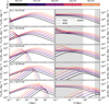 |
Fig. 3. Density profiles (left column) and projected density contrasts (right column) of halos of different mass (color coded) at redshift z = 1 for different ULA particle masses (rows) in the extreme case of a ULA-only dark matter sector. Full lines show the total profiles, dashed lines show the corresponding cold dark matter profiles (assumed to follow a Navarro-Frenk-White profile), and dotted lines show the soliton core profile. In the right column, we highlight the scales we use for the weak lensing measurement in white. |
In this section and for this demonstration, we use the Navarro-Frenk-White profile for the collisionless part of the profile (Navarro et al. 1996) given by
 (20)
(20)
with scale radius rs and normalization ρ0. We set these values as follows: For a given halo mass and redshift, we computed the radius r500c using the definition for spherical overdensity masses and the mean concentration c500c following the relation by Ragagnin et al. (2021). This sets rs = r500c/c500c. Using the profile to compute the mass enclosed in r500c, we set the normalization constant ρ0 in accordance with Eq. 4 in Navarro et al. (1996) adjusted to the overdensity 500.
We constructed the composite model following the recommendations by May & Springel (2023). The transition radius rt from a soliton core to the collisionless profiles is defined by the condition ρNFW(rt) = ρsoli(rt). If for small ULA masses (ma < 10−24 eV) no rt satisfies this condition, we pick rt = max(r2ρsoli). If there are two solutions, we picked the larger of the two. The total profile was constructed as
 (21)
(21)
May & Springel (2023) discusses that this model is only qualitatively correct for spherically averaged profiles. As such, it is not suited for our precise weak lensing measurements and can only be used to understand the phenomenological effect of ULA particles on massive halo profiles. In the left column of Fig. 3, we show the resulting total mass profiles for different ULA masses ma and halo masses M.
However, the density profile is not directly observable by the weak gravitational lensing signal, which is sourced by the projected density contrast
 (22)
(22)
where R is the 2D cluster centric distance, and  , the projected matter density. The transformation from a 3D density profile to a density contrast is nonlocal, as weak lensing depends on the enclosed mass. Flat density profiles thus provide very little signal, while the effect of central overdensity can be observed well outside of their physical extent. These density contrasts are shown in the right panel of Fig. 3.
In this extreme case of a ULA-only dark matter sector, two interesting regimes can be observed. For intermediate ULA masses around ma = 10−24 eV pronounced soliton cores in the innermost part of the halos appear. Nonetheless, this effect is not observable by our weak lensing measurements, which are restricted to scales around ∼1 Mpc (highlighted in white in the right panel of Fig. 3). Small ULA particle masses ma ≲ 10−26 eV are a second interesting regime. For these ULA masses, cores become so extended that they dominate the density profile for group-scale halos. At ma ∼ 10−27 eV, also cluster scale halos with M < 1014 M⊙ are dominated by cores. This observation can be interpreted in terms of the soliton radius. If it becomes larger than the cluster size, axions no longer cluster in the halo. This is the ULA mass range we refer to as the dark energy regime. In this context, the light axions, because of their flat inner profile shape, provide a vanishing weak lensing signal. In all cases, the excess surface mass density described by Equation (22) is mostly unaffected. Furthermore, the effect on ΔΣ is, as expected, more noticeable for low-mass halos (M ∼ 1013 M⊙). The eRASS1 cosmological sample has a median mass of Mmed = 1014.39 M⊙ while 90% of the halos have a mass larger than 1014 M⊙. We therefore conclude that even a pure ULA dark matter sector for ma ≳ 10−26 eV does not significantly impact the prediction for the weak lensing signal of group and cluster scale halos, as compared to a Navarro-Frenk-White profile. Quantitative predictions for the weak lensing signal of groups and clusters would require large-volume hydro-dynamical simulations in ULA cosmology, which are not available to date, and therefore cannot be incorporated in this work. These considerations are left for future works.
Finally, in a mixed ULA-cold dark matter model, N-body simulations by Schwabe et al. (2020) show that soliton cores are formed for ULA fractions higher than Ωa/(Ωm + Ωa)≳0.1. However, below this fraction, these simulations show no evidence of the formation of soliton cores. Below ULA masses of ma ≲ 10−28 eV, ULAs are in the dark energy regime and do not contribute to the WL signal (see Sect. 2.4).
We conclude that the weak lensing mass calibration remains valid throughout the full ULA mass range as long as the ULA fraction remains below the aforementioned threshold. Hence, we use the profile described in Grandis et al. (2024).
4.5. Mixture model
The eRASS1 cluster catalog contains three classes of objects: galaxy clusters (C), which are of interest, and active galactic nuclei (AGN), as well as background fluctuations misclassified as clusters (NC), the latter two considered contaminants. Our model simultaneously accounts for the cluster counts and the contaminant fractions through the Poisson mixture model, as described in detail in Kluge et al. (2024). The total density is the sum of the three-component model:
 (23)
(23)
In terms of the total number of objects in each class, we obtained
 (24)
(24)
where fAGN and fNC are the respective fractions of contaminants. Consequently, we can express the number of AGN, false detections, and the total number of objects in the catalog as a function of the cosmology-dependent number of clusters NC:
 (25)
(25)
Starting from the formalism above, we can write the total number of objects as
 (26)
(26)
and that the number density of contaminants follows λAGN(x|θ) = NAGN(Θ)𝒫AGN(x), and λNC(x|θ) = NNC(Θ)𝒫NC(x). In this equation, 𝒫 describes the probability distribution function of the respective object, depending on the observables. Finally, the likelihood becomes
 (27)
(27)
The contaminant fractions fAGN and fNC are fit for during the parameter inference.
4.6. Integration of ultralight axions
Constraining the ULA fraction requires us to predict the massive dark matter halo number density in the corresponding model. We introduce ULAs in the cluster abundance cosmological pipeline by implementing a modified version of the power spectrum used to produce the HMF (Diehl & Weller 2021). This framework provides us with the proper transfer function and growth of structure models. In practice, we use axionCAMB (Grin et al. 2022), a modified version of CAMB that adds the evolution of primordial density fluctuations caused by an axion field to the Boltzmann solver. The effect of ULAs on the HMF is illustrated in Fig. 4 for different ULA masses ma and ULA relic densities Ωa. We use axionCAMB to modify the Hubble rate as a function of redshift H(z) for a universe with dark matter composed of ULAs. Using an updated Hubble rate ensures that we properly account for the redshift dependence of the Hubble rate on the effective properties of ULAs (dark energy or dark matter behavior in the Hubble rate) when computing the distances between background galaxies and the lens (or the observer) needed for the weak gravitational lensing calibration of the scaling laws a described in Sect. 4.4. Fig. 5 shows the influence of ULA mass on the Hubble rate in a cosmology with a high ULA abundance as dark matter. We also use axionCAMB to compute the matter power spectrum. We then compute the r.m.s. density fluctuations (Eq. (9)) and use them as input to the multiplicity function f(σ) from Tinker et al. (2008) to compute the halo number density.
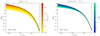 |
Fig. 4. Halo mass function with Planck Collaboration VI (2020) cosmological values (ΩΛ ≈ 0.7, Ωm + Ωa ≈ 0.3) at z = 0.1 with a fixed relative ULA density of Ωa/(Ωcdm + Ωa) = 0.5 and varying ULA mass (left) and a fixed ULA mass of ma = 10−25 eV and varying ULA abundance (right) compared to the ΛCDM HMF (black). Low-mass halo suppression becomes stronger with decreasing ULA mass and increasing ULA abundance. For higher ULA masses of ma ≳ 10−24 eV, the HMF becomes indistinguishable from the one in a ΛCDM cosmology, as is the case for Ωa → 0. |
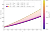 |
Fig. 5. Hubble rate |
Consequently, in this work, we choose to model the effect of ULAs solely by implementing the power spectrum produced by the corresponding ULA model in the HMF obtained by Tinker et al. (2008). The impact of ULAs is thus obtained through the transfer function and the growth of structure used to compute the r.m.s. density fluctuations in Equation (9). However, accounting for ULAs also requires recalculating the critical overdensity for halo collapse, given that they do not form structures below the Jeans mass. Different studies in the literature have provided fitting functions to model this effect, with smoothed k window functions (Bohr et al. 2021), or analytical formulas (Dome et al. 2025). However, these methods have not been tested in the framework of cosmological parameter inference. Additionally, most of the correcting effects are significant at masses much below the mass range of clusters below the detection limits of the galaxy cluster catalogs of the eROSITA All-Sky Survey (∼1010 M⊙ for the typical ranges of the corrections, compared with ∼1014 M⊙ for a typical cluster detected in eRASS1). Consequently, it is not necessary to apply these corrections for the eRASS1 sample. We note that better modeling will be required to extend the analysis to a lower-mass range below M ≲ 1013 M⊙.
Below an ULA mass of 10−28 eV, we exclude ULAs from the matter density in the HMF formalism to account for the fact that their de Broglie wavelength exceeds the Jeans length and ULAs are not expected to contribute to halo formation in this regime. For ULA masses of log10(ma[eV]) ≲ −32.5, the de Broglie wavelength of the ULA BEC exceeds the size of the universe, making ULAs indistinguishable from a cosmological constant Λ. As such, a model is indistinguishable from ΛCDM, we exclude this regime from our analysis.
For ULA masses −32.5 ≲ log10(ma[eV]) ≲ −31.5, despite not contributing to halo formation, ULAs affect the Hubble rate, which in turn influences the distance measurements relevant for the weak lensing calibration. Above log10(ma[eV]) ∼ −32.5, only objects at redshifts higher than z = 0.8 (maximum redshift for galaxy clusters in the eRASS1 cosmology sample) are affected by the regime change in the Hubble rate. This involves the galaxies used for the gravitational weak lensing calibration of the scaling relations (see Sect. 4.4 for details) that extend up to z ≲ 6 in redshift space. We consider this effect by computing the distances based on the ULA Hubble rate extracted from axionCAMB in this regime. All ULA mass bins above the lowest-mass bin are not affected by the regime change in the Hubble rate, i.e., ULA masses above log10(ma[eV]) ≲ −31.5 (see Fig. 2 for further details). Fig. 5 illustrates how the regime affects the Hubble rate in a cosmology with a high ULA abundance as a function of ULA mass (color coded).
5. Results and discussion
In this section, we present the results of the Bayesian inference fitting of cosmological and ULA parameters through galaxy cluster number counts. We used the X-ray count rate, the optical richness, and (where available) the reduced tangential shear profiles given in the eRASS1 galaxy cluster cosmology catalog.
5.1. Consistency checks
We implement several changes to the base cosmological pipeline of G24 as described in detail in Sect. 4. To ensure the adaptations do not introduce inconsistencies, we reproduce the main cosmological results in the new ultralight axion framework by choosing fixed ULA parameters, which are indistinguishable from a ΛCDM cosmology. This limit can be achieved either by setting the ULA relic density to Ωa = 0 or for values log10(ma[eV]) ≳ −18 (see Fig. 1 and Fig. 4). The code axionCAMB only allows positive values for Ωa, so we chose Ωa = 10−9, several orders of magnitude below any other cosmological fluid component in the relevant redshift range. We additionally fix the ULA mass to log10(ma[eV]) = −12. The matter power spectrum and hence σ(M, z) with this choice of ULA parameters is in perfect agreement with the ΛCDM quantities. We checked that running the adapted pipeline leads to almost identical results as compared to the ones obtained in the ΛCDM case shown in G24. A subset of the obtained cosmological parameters is presented in Fig. 6. We conclude that the applied changes did not introduce inconsistencies with the main cosmological results from eRASS1.
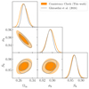 |
Fig. 6. Consistency check: Posteriors for the cosmological parameters Ωm, σ8, and S8 in the ΛCDM (ma = 10−12 eV and Ωa = 10−9). These values were chosen arbitrarily such that they satisfy ma ≫ 10−18 eV and Ωa ≪ 10−3. The results are consistent with G24. The inner and outer contours represent the 68% and 95% contour levels, respectively. |
5.2. Cosmological constraints
Following the approach developed by Hložek et al. (2018) and Rogers et al. (2023), we perform a binned analysis in the logarithmic ULA mass log10(ma[eV]). We consider a total of nine bins, from log10(ma[eV]) = −24 in the highest-mass bin to log10(ma[eV]) = −32. Independent cosmological and scaling relation parameters are considered within each ULA mass bin. The analysis is not sensitive to how the ULA mass is treated within a mass bin, as drawing the ULA mass randomly within a bin or fixing it to the central bin value does not influence the posterior distribution.
We assumed a flat (ΛCDM+ ULA) cosmology with massless neutrinos to get a conservative estimate of the effect of ULAs. We leave the matter energy density fraction at redshift z = 0, Ωm, the baryon energy density fraction at redshift z = 0, Ωb, the scalar spectral index, ns, the normalization of the matter power spectrum, log(As), and the Hubble constant, H0, free. We leave the same parameters free for the scaling relations as done in G24. The priors on the cosmological parameters are shown in Table 1.
Cosmological parameters and priors.
For all mass bins except the one with m = 10−25 eV, we find no deviations from the ΛCDM cosmological posteriors obtained by G24, and the posteriors are in good agreement between the different ULA mass bins. We show the cosmological posterior distributions for the cosmological parameters Ωm, σ8, and S8 for a subset of ULA mass bins covering the full mass range in Fig. 7.
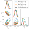 |
Fig. 7. Posterior distributions for Ωm, σ8, and S8 in a subset of ULA mass bins. We find consistent cosmological constraints across all mass bins within 1σ (except for the excluded ma = 10−25 eV mass bin). The results are furthermore compatible with G24. The inner and outer contours represent the 68% and 95% contour levels, respectively. |
In the mass bin around ma = 10−25 eV (i.e., covering the range 10−25.5 eV ≤ ma ≤ 10−24.5 eV), we find significant discrepancies compared to G24 in the X-ray and optical scaling relation parameters (e.g., the discrepancy between AX and GX is 10.9σ, the discrepancy between Aλ and Cλ is 8.0σ). Figure 8 shows the posterior distributions of both the X-ray and optical scaling relations, comparing a representative selection of ULA mass bins with G24. The scaling relations, together with the gravitational weak lensing calibration, translate the observed count-rates and optical richnesses to the total masses of the clusters in the eRASS1 sample. Together with the contamination model and the selection function, these relations include all astrophysical modeling between observation and theory. As demonstrated in Sect. 4.4, ULAs do not alter the weak lensing signal compared to the ΛCDM scenario in the ma = 10−25 eV mass bin. Consequently, the astrophysical modeling should be independent from the abundance of ULAs with a mass around ma = 10−25 eV, i.e., the scaling relation parameter posteriors should be comparable with the ones reported by G24. However, in contrast to all other ULA mass bins, this is not the case for the ma = 10−25 eV bin (see Fig. 8). Thus, the cosmological parameters and the ULA relic density in this bin are not reliable, which is why we opt to exclude the ma = 10−25 eV mass bin from the analysis.
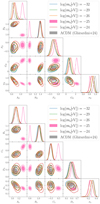 |
Fig. 8. Posterior distributions in a representative subset of ULA mass bins for the X-ray scaling relations (top) and the optical scaling relations (bottom). The large discrepancies in the astrophysical scaling relation model parameters between the ma = 10−25 eV mass bin on the one hand and G24 and the remaining mass bins on the other hand indicates an unphysical posterior distribution in the ma = 10−25 eV ULA mass bin. Consequently, the concerned mass bin is excluded from the analysis. |
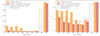 |
Fig. 9. Upper bounds on the relative ULA density Ωa in each logarithmic ULA mass bin. The left plot shows the upper bounds on Ωa on a linear scale, and the right plot shows the upper bounds on a logarithmic scale. The bar height indicates the 95% confidence interval. The orange bars indicate the bounds obtained by eRASS1 galaxy clusters only, and the gray hatched bars show the bounds obtained from Planck 2015 CMB data by Hložek et al. (2018). The red bars show the bounds obtained from combining the bounds from eRASS1 galaxy clusters with those from Planck 2015 CMB data. |
Furthermore, we find that the posterior distribution is highly sensitive to the choice of priors, indicating a lack of statistical robustness in the ma = 10−25 eV ULA mass bin. However, we report no constraining power on the ULA relic density in this bin for prior choices comparable to those used by G24, similar to the results for the ma = 10−24 eV mass bin. Consequently, the ma = 10−25 eV mass bin does not contribute to constraining the ULA fraction. Possible reasons for the reported discrepancies include a breakdown of the HMF fitting function or the modeling of the shear signal for this specific ULA mass range. A detailed understanding of this effect will require further investigation beyond the scope of this work. In the figures with an interpolated curve between the bin values (Figs. 11, 13), we assume the Planck upper confidence level (Hložek et al. 2018) as a reasonable reference point for a bin with lacking constraining power for interpolation purposes only.
5.3. Constraints on the ULA parameter space
We found an exclusion region for ULAs by performing a binned analysis, providing upper bounds on the relic density within logarithmic mass bins. Since ULAs form BECs with characteristic extensions given by their thermal de Broglie wavelengths λdB ∼ 1/ma, ULAs with different masses have imprints on different corresponding scales. Ultralight axions with masses of order 𝒪(10−22 eV) have de Broglie wavelengths of order 𝒪(kpc), while ULAs with masses of order 𝒪(10−33 eV) have de Broglie wavelengths comparable to the size of the universe. As galaxy clusters are probing the 𝒪(Mpc) scales and above, their abundance can constrain ULAs with masses of order 𝒪(10−26 eV) and below. The inverse relation between scale and ULA mass highlights the importance of galaxy groups in the sample to explore higher ULA mass regimes. Very light ULAs with masses of order 𝒪(10−33 eV) mimic a dark energy component, as BECs on the scale of the universe add a global energy component to the universe. Ultralight axions with masses slightly above this threshold undergo a transition from an effective dark energy component to an effective dark matter component at some redshift where the size of the universe exceeds the de Broglie wavelength of the ULA condensate. For this regime, no models exist for halo collapse in the presence of ULAs. Hence, we are not able to probe this region and exclude ULA masses log10(ma[eV]) < −32.5 from our analysis.
We find upper bounds on the ULA relic density Ωa obtained from binning the logarithmic ULA mass with a bin width of Δlog10(ma[eV]) = 1 around powers of ten. We treat each bin independently. We find upper bounds on the ULA relic density in each ULA mass bin with log10(ma[eV]) ≤ −26, as presented in Fig. 9. We confirm the exclusion region below the log10(ma[eV]) = −25 mass bin, which has been reported by Hložek et al. (2015, 2018), and Rogers et al. (2023). eRASS1 galaxy cluster abundance alone yields the tightest constraints on the ULA relic density in the mass bins log10(ma[eV]) ∈ { − 27, −26} with
![Mathematical equation: $$ \begin{aligned} {\Omega _{\rm a}}(-26.5<\log _{10}(m_{\rm a}[\mathrm{eV}])\le -25.5)&< 0.0079,\nonumber \\ {\Omega _{\rm a}}(-27.5<\log _{10}(m_{\rm a}[\mathrm{eV}])\le -26.5)&< 0.0035, \end{aligned} $$](/articles/aa/full_html/2025/12/aa54045-25/aa54045-25-eq41.gif) (28)
(28)
both at a 95% confidence level. Fig. 10 shows that these are the tightest upper bounds that have been presented in the literature. Combining our results with the available chains from Planck 2015 CMB data (Hložek et al. 2018), we find even tighter constraints in both mass bins:
![Mathematical equation: $$ \begin{aligned} {\Omega _{\rm a}}(-26.5<\log _{10}(m_{\rm a}[\mathrm{eV}])\le -25.5)&< 0.0058,\nonumber \\ {\Omega _{\rm a}}(-27.5<\log _{10}(m_{\rm a}[\mathrm{eV}])\le -26.5)&< 0.0030. \end{aligned} $$](/articles/aa/full_html/2025/12/aa54045-25/aa54045-25-eq42.gif) (29)
(29)
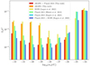 |
Fig. 10. Comparison of ULA constraints obtained from eRASS1 galaxy cluster abundance (this work), Planck 2015 (Hložek et al. 2018), and 2018 CMB data; BOSS galaxy clustering data (both by Rogers et al. 2023); and combined analyses of eRASS1 and Planck 2015 (this work) and Planck 2018 and BOSS (Rogers et al. 2023). The bar height indicates the 95% exclusion limits of the ULA density Ωa times h2 = (H0/100)2 in each log10(ma[eV]) bin. eRASS1 yields the tightest upper bounds on dark matter ultralight axions in the log10(ma[eV]) ∈ { − 27, −26} bins. |
From eRASS1 galaxy cluster number counts alone, we find that the ULA relic density Ωa cannot exceed 2.7% of the total energy density of the universe for ma ≤ 10−27.5 eV and is bound below 0.84% for ULA masses 10−27.5 eV ≤ ma ≤ 10−26.5 eV and below 0.36% for ULA masses 10−26.5 eV ≤ ma ≤ 10−25.5 eV. A significant contribution of ULAs to the total dark matter density can thus be ruled out by the growth of structure as observed through eRASS1 galaxy cluster number counts.
It is particularly interesting to compare the eRASS1 cluster number count constraints with those found using BOSS galaxy clustering data as another large-scale structure probe. Rogers et al. (2023) studied the cosmological implications of ULAs using the twelfth data release of the Baryon Oscillation Spectroscopic Survey (BOSS) catalog (Dawson et al. 2013; Alam et al. 2017) and found upper bounds on the ULA fraction in a binned analysis in the range −32 ≤ log10(ma[eV]) ≤ −26. As expected, galaxy clustering and galaxy cluster number counts constrain different ULA mass regimes. This is due to the relation between the ULA mass and the scale it affects: The heavier the ULA, the larger the affected scale in the matter power spectrum, for instance, a ULA with a mass of ∼10−24 eV is only observable on scales below ∼200 kpc, while a ULA with a mass of ∼10−25 eV is already observable on scales ∼500 kpc and below (see Fig. 1). While, in comparison to other probes, Rogers et al. (2023) find the tightest constraints (Ωah2 < 0.0418) in the ULA mass bin around ma = 10−25 eV, corresponding to an effect on smaller scales, eRASS1 cluster number counts yield the tightest constraints among complementary in the mass bins ma ∈ {10−27 eV, 10−26 eV}. Ultralight axions in this mass range affect larger scales, which is constrainable using galaxy cluster number counts. Similar to galaxy clustering data, eRASS1 cluster number counts have reduced constraining power at scales extending the typical probe scales, as seen in the lowest-mass bins. On these largest scales (corresponding to ULA masses ma ≲ 10−28 eV), CMB measurements by the Planck collaboration (Planck Collaboration XIII 2016; Planck Collaboration VI 2020) have the highest constraining power and yield the tightest constraints (Hložek et al. 2015, 2018; Rogers et al. 2023). For better comparison with the results obtained using other probes (see Fig. 10), we also provide the bounds of each constraining bin for Ωa and Ωah2 in Table 2.
Upper bounds on the ULA relic density (Ωa) and Ωah2 at the 95% confidence level in each constraining mass bin for eRASS1 cluster number counts only and when combined with Planck 2015 CMB data.
We emphasize that the weak lensing mass calibration as described in Sect. 4.4 remains valid over the full considered ULA mass range as the 95% confidence levels do not exceed ULA fractions of Ωa/(Ωm + Ωa)≈0.1 for ma ≲ 10−26 eV, and below ma ≈ 10−28.5 eV, ULAs are not included in the HMF model and thus the modeling used in G24 remains valid. For higher ULA masses, Sect. 4.4 justifies the modeling choice of keeping NFW profiles for the weak lensing mass calibration up to any ULA fraction.
Our current pipeline is limited by the model of the halo abundance in ULA cosmology, where we use a modified power spectrum in the Tinker et al. (2008) fitting function. Although this is justified by numerical simulations (see Sect. 4.6), our results will be improved if suitable emulators are developed for this model. Additionally, for this pioneering work, we fix the masses of the neutrinos, while the effect of neutrinos is degenerate with ULAs. This modeling choice results in our constraints being conservative upper limits. Including massive neutrinos in the next analyses significantly tightened our constraints.
5.4. Forecasts for the deepest eROSITA survey
This section presents an estimation quantifying the potential of future galaxy cluster samples, illustrated by the deepest eROSITA All-Sky Surveys. The constraints presented in this work are based on eRASS1, which represents ∼22% of the stacked consequent eROSITA All-Sky Survey (eRASS:5, hereafter). In the near future, the release of deeper eROSITA data and associated catalogs will significantly increase the number of available galaxy clusters and groups. In particular, we expect the number of low-mass galaxy groups to increase significantly with higher exposure time. To assess the expected evolution of cluster abundance in future eROSITA data releases, we generate a mock sample representing a catalog for eRASS:5. This mock catalog is constructed using the methodology outlined in G24 to validate the pipeline.
We generated a dark matter halo catalog with the cosmology inferred in G24, using the halo mass function from Tinker et al. (2008). We then create mock X-ray and optical observables following the scaling relations described in Section 4.1. We then select the fraction of objects that would be detected using the selection function described in Clerc et al. (2024). The X-ray selection function depends on X-ray count rates, hydrogen column density, background, and exposure time. We scale the exposure time by a factor of 4.6 to simulate a survey with 4.6 times the depth of eRASS1. The result is a catalog containing ∼15 000 clusters with 0.1 < z < 0.8. Figure 12 presents the cluster abundance in eRASS1 and in the mock eRASS:5 catalog. In the deeper eROSITA survey, the statistical power of cosmological constraints will be driven by the detection of a large and significant sample of galaxy groups. At 1013.8 M⊙, we detect approximately five times more massive clusters than in eRASS1, where the constraints on the parameter space are mostly constrained by the number of lower-mass galaxy clusters and galaxy groups (see Fig. 4).
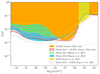 |
Fig. 11. Exclusion regions (95% confidence level) in the log10(ma[eV]) − Ωah2 space as constrained by different probes. Colored regions represent the part of the parameter space where one ULA species can be excluded at 95% confidence level, whereas white regions represent the unconstrained parameter space. eRASS1 galaxy cluster number counts (orange) exclude a new region in the parameter space between 10−27.5 eV ≲ ma ≲ 10−26 eV, corresponding to galaxy cluster scales. Combining eRASS1 galaxy cluster number counts with the Planck 2015 CMB data (red) further improves the eRASS1 bounds on the ULA relic density. For ULA masses below ma ≲ 10−28 eV, Planck 2018 CMB data yields the tightest bounds. Above ma ≳ 10−25 eV, galaxy clustering data from BOSS yields the tightest constraints. The curves are interpolated between the central bin values, which represent the 95% confidence levels in the respective bins. In the ma = 10−25 eV mass bin, the Planck upper confidence level has been assumed as a reasonable choice for the interpolation (for details on that bin, see Sect. 5.2). |
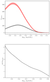 |
Fig. 12. Forecasts for an eRASS:5 survey. Left: Number count of X-ray detected clusters for an eRASS:5 survey (red) compared with an eRASS1 catalog (black). The Poisson error bars are represented by filled lines. Right: Relative difference of eRASS:5 detected clusters and eRASS1 detected objects. eRASS:5 will contain five times more clusters at M = 1013.8 M⊙. |
We assumed that the Poisson error of the cluster abundance is the main statistical limiting factor. This means that we assume that the additional low-mass objects possess X-ray, optical, and weak lensing quantities measured as precisely as the ones obtained for massive clusters. We provide an optimistic and a pessimistic scenario based on the potential inclusion of low-mass clusters in Fig. 13. In the optimistic case, our lower limit decreases by a factor of 2.2, while it is lowered by a factor of 1.7 in the pessimistic case. The reliability of our forecasts for the eRASS:5 data is influenced by the accuracy of the selection function; the robustness of the model used to predict the abundance, including the HMF model; the universality of the scaling relations over the full survey mass range; and the precision of forthcoming weak lensing measurements for the mass calibration of low-mass galaxy groups.
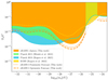 |
Fig. 13. Forecast for eRASS:5 data. The exclusion region of the ULA parameter space obtained from eRASS:5 mock catalog is presented with the orange dotted line for a pessimistic scenario and with the orange dashed line for an optimistic scenario, and can be compared with the plain orange region corresponding to the exclusion region obtained by eRASS1. For the missing bin, the Planck upper confidence level was assumed for the interpolation (see Sect. 5.2). |
6. Conclusions
The unique properties of ULAs lead to observable phenomena such as solitonic cores in dark matter halos and interference patterns on cosmological scales. These features can be probed through astrophysical observations, providing potential evidence of their existence.
Galaxy cluster number counts inferred from the eRASS1 cluster cosmology catalog (Bulbul et al. 2024; Kluge et al. 2024) can be used to test and constrain the viable dark matter candidates, such as ULAs, through the evolution of the structure growth. Indeed, eRASS1, being the largest ICM-selected sample to date, has a significant constraining power. Additionally, it has the potential to probe the group regime, which is very sensitive to dark matter signatures.
In this work, we performed Bayesian inference on cosmological parameters in a universe with an additional ULA component parameterized by the logarithmic ULA mass and ULA relic density {log10(ma[eV]), Ωa}. The matter power spectrum was computed by axionCAMB (Hložek et al. 2015), from which we computed the HMF using the multiplicity function by Tinker et al. (2008). The forward modeling process requires the selection function developed by Clerc et al. (2024) and additional parameters from the mixture model that take care of possible contaminants, the count-rate-mass scaling relation, and the richness-mass scaling relation, which are calibrated by gravitational weak lensing shear maps (Grandis et al. 2024). Apart from the adaptations described in Sect. 4.6, we used the framework established in G24 for the parameter inference.
We performed a binned analysis with logarithmic ULA mass bins covering the whole mass spectrum of ultralight axions from the dark matter regime starting at log10(ma[eV]) = −24 down to the dark energy regime with the lowest ULA mass at log10(ma[eV]) = −32 including an independent full cosmological inference in each bin while assuming a flat universe. We constrained the following set of cosmological parameters: the matter relic density, Ωm, and the normalization of the matter power spectrum, log(As). We left the Hubble constant, H0; the scalar spectral index, ns; and the baryon relic density, Ωb, free but could constrain them as done in G24. We chose a uniform prior on Ωa between 0 and 1 in both scenarios. All common parameters have the same priors as in G24.
We performed a consistency check with the eRASS1 cosmological results from G24 by fixing ULA parameter values to log10(ma[eV]) ≫ −18 and Ωa → 0, effectively switching off the effect of ULAs on structure growth. The results are consistent with G24, indicating that including ULAs does preserve the correctness and reliability of the inference framework.
The binned analysis of eRASS1 galaxy cluster number counts alone yields tight bounds on the ULA relic density, especially in the two highest ULA mass bins within the exclusion region log10(ma[eV]) ∈ { − 27, −26}. This ULA mass range corresponds to physical scales (de Broglie wavelengths) of ULA BECs comparable to the typical galaxy cluster scales around 1 Mpc to 10 Mpc. The parameter space excluded by eRASS1 galaxy clusters in comparison to complementary probes is shown in Fig. 11. In the mass range of 10−27.5 eV ≤ ma ≤ 10−26.5 eV, the upper limit on the ULA relic density is Ωa < 0.0036 of the total energy density of the universe. Similarly, in the mass range of 10−26.5 eV ≤ ma ≤ 10−25.5 eV, the ULA relic density is constrained to Ωa < 0.0084 of the total energy density of the universe. The ma = 10−25 eV mass bin was excluded from the analysis due to a lack of modeling and statistical robustness in that particular bin. In the mass regime 10−32.5 eV ≤ ma ≤ 10−27.5 eV, the ULA relic density is bound below Ωa ≲ 0.055. We conclude that the evolution of structure growth as observed by eRASS1 galaxy cluster number counts rules out ULAs as a significant contribution to the total dark matter density of the Universe. The constraints on the abundance at different confidence levels concerning a logarithmic ULA mass bin are presented in Fig. 9. Overall, these results highlight the potential of cluster abundance measurements and the evolution of the growth of structure as a probe of ULAs. For the first time, we have obtained constraints using cluster abundance in a redshift and scale regime complementary to the one probed by other cosmological probes.
In the near future, statistically more powerful cosmological simulations, including ULAs (or ultralight scalar fields, fuzzy dark matter) that predict an HMF model and shear profiles for a sufficiently large cosmological parameter space, will be required to provide unbiased constraints. We note that the constraints presented in this work were obtained using the eRASS1 cosmology sample of 5 259 X-ray-selected massive clusters. The primary sample contains a higher fraction of low-mass objects, so we are more sensitive to ULA signatures, provided that we carefully model the baryonic systematic effects that affect groups. Future analyses of deeper surveys with eROSITA at eRASS:5 depth will provide larger samples of low-mass halos with a greater constraining power in the ULA parameter space, improving the overall constraints by a factor of 1.7.
Acknowledgments
The authors thank the referee for the helpful and constructive comments on the draft. We further thank Christian Garrel for his contributions to the codebase and the valuable exchange with him. Thanks to Johannes Diehl, Julia Sisk-Reynes, and Luis A. Ureña-López for the helpful discussions. This work is based on data from eROSITA, the soft X-ray instrument aboard SRG, a joint Russian-German science mission supported by the Russian Space Agency (Roskosmos), in the interests of the Russian Academy of Sciences represented by its Space Research Institute (IKI), and the Deutsches Zentrum für Luft und Raumfahrt (DLR). The SRG spacecraft was built by Lavochkin Association (NPOL) and its subcontractors and is operated by NPOL with support from the Max Planck Institute for Extraterrestrial Physics (MPE). The development and construction of the eROSITA X-ray instrument was led by MPE, with contributions from the Dr. Karl Remeis Observatory Bamberg & ECAP (FAU Erlangen-Nuernberg), the University of Hamburg Observatory, the Leibniz Institute for Astrophysics Potsdam (AIP), and the Institute for Astronomy and Astrophysics of the University of Tübingen, with the support of DLR and the Max Planck Society. The Argelander Institute for Astronomy of the University of Bonn and the Ludwig Maximilians Universität Munich also participated in the science preparation for eROSITA. The eROSITA data shown here were processed using the eSASS software system developed by the German eROSITA consortium. S. Zelmer, E. Bulbul, V. Ghirardini, A. Liu, and X. Zhang acknowledge financial support from the European Research Council (ERC) Consolidator Grant under the European Union’s Horizon 2020 research and innovation program (grant agreement CoG DarkQuest No 101002585). N. Clerc was financially supported by CNES. T. Schrabback and F. Kleinebreil acknowledge support from the German Federal Ministry for Economic Affairs and Energy (BMWi) provided through DLR under projects 50OR2002, 50OR2106, and 50OR2302, as well as the support provided by the Deutsche Forschungsgemeinschaft (DFG, German Research Foundation) under grant 415537506. M. Brüggen acknowledges funding by the Deutsche Forschungsgemeinschaft (DFG, German Research Foundation) under Germany’s Excellence Strategy – EXC 2121 “Quantum Universe” – 390833306. S. Krippendorf’s work has been partially supported by STFC consolidated grants ST/T000694/1 and ST/X000664/1.
References
- Abbott, T. M. C., Allam, S., Andersen, P., et al. 2019, ApJ, 872, L30 [Google Scholar]
- Abbott, T. M. C., Aguena, M., Alarcon, A., et al. 2022, Phys. Rev. D, 105, 023520 [CrossRef] [Google Scholar]
- Abel, C., Afach, S., Ayres, N. J., et al. 2020, Phys. Rev. Lett., 124, 081803 [CrossRef] [PubMed] [Google Scholar]
- Adame, A. G., Aguilar, J., Ahlen, S., et al. 2025, JCAP, 2025, 021 [CrossRef] [Google Scholar]
- Aihara, H., Arimoto, N., Armstrong, R., et al. 2018, PASJ, 70, S4 [NASA ADS] [Google Scholar]
- Alam, S., Ata, M., Bailey, S., et al. 2017, MNRAS, 470, 2617 [Google Scholar]
- Amon, A., Gruen, D., Troxel, M. A., et al. 2022, Phys. Rev. D, 105, 023514 [NASA ADS] [CrossRef] [Google Scholar]
- Artis, E., Ghirardini, V., Bulbul, E., et al. 2024, A&A, 691, A301 [NASA ADS] [CrossRef] [EDP Sciences] [Google Scholar]
- Artis, E., Bulbul, E., Grandis, S., et al. 2025, A&A, 696, A5 [NASA ADS] [CrossRef] [EDP Sciences] [Google Scholar]
- Arvanitaki, A., Dimopoulos, S., Dubovsky, S., Kaloper, N., & March-Russell, J. 2010a, Phys. Rev. D, 81, 123530 [NASA ADS] [CrossRef] [Google Scholar]
- Arvanitaki, A., Dimopoulos, S., Dubovsky, S., Kaloper, N., & March-Russell, J. 2010b, Phys. Rev. D, 81, 123530 [NASA ADS] [CrossRef] [Google Scholar]
- Arvanitaki, A., Baryakhtar, M., & Huang, X. 2015, Phys. Rev. D, 91, 084011 [Google Scholar]
- Asgari, M., Lin, C.-A., Joachimi, B., et al. 2021, A&A, 645, A104 [NASA ADS] [CrossRef] [EDP Sciences] [Google Scholar]
- Becker, M. R., & Kravtsov, A. V. 2011, ApJ, 740, 25 [NASA ADS] [CrossRef] [Google Scholar]
- Bocquet, S., Grandis, S., Bleem, L. E., et al. 2024, Phys. Rev. D, 110, 083510 [NASA ADS] [CrossRef] [Google Scholar]
- Bohr, S., Zavala, J., Cyr-Racine, F.-Y., & Vogelsberger, M. 2021, MNRAS, 506, 128 [CrossRef] [Google Scholar]
- Brout, D., Scolnic, D., Popovic, B., et al. 2022, ApJ, 938, 110 [NASA ADS] [CrossRef] [Google Scholar]
- Bulbul, E., Markevitch, M., Foster, A., et al. 2014, ApJ, 789, 13 [NASA ADS] [CrossRef] [Google Scholar]
- Bulbul, E., Liu, A., Kluge, M., et al. 2024, A&A, 685, A106 [NASA ADS] [CrossRef] [EDP Sciences] [Google Scholar]
- Bullock, J. S., & Boylan-Kolchin, M. 2017, ARA&A, 55, 343 [Google Scholar]
- Cardoso, V., Dias, Ó. J. C., Hartnett, G. S., et al. 2018, JCAP, 2018, 043 [CrossRef] [Google Scholar]
- Chiu, I. N., Ghirardini, V., Liu, A., et al. 2022, A&A, 661, A11 [NASA ADS] [CrossRef] [EDP Sciences] [Google Scholar]
- Chiu, I. N., Ghirardini, V., Grandis, S., et al. 2025, A&A, 704, A110 [NASA ADS] [CrossRef] [EDP Sciences] [Google Scholar]
- Clerc, N., Comparat, J., Seppi, R., et al. 2024, A&A, 687, A238 [NASA ADS] [CrossRef] [EDP Sciences] [Google Scholar]
- Comparat, J., Eckert, D., Finoguenov, A., et al. 2020, Open J. Astrophys., 3, 13 [Google Scholar]
- Conlon, J. P. 2006, J. High Energy Phys., 2006, 078 [Google Scholar]
- Conlon, J. P., Day, F., Jennings, N., Krippendorf, S., & Rummel, M. 2017, JCAP, 2017, 005 [Google Scholar]
- Costanzi, M., Saro, A., Bocquet, S., et al. 2021, Phys. Rev. D, 103, 043522 [Google Scholar]
- Crewther, R. J., di Vecchia, P., Veneziano, G., & Witten, E. 1979, Phys. Lett. B, 88, 123 [Google Scholar]
- Dalal, N., & Kravtsov, A. 2022, Phys. Rev. D, 106, 063517 [NASA ADS] [CrossRef] [Google Scholar]
- Dalal, R., Li, X., Nicola, A., et al. 2023, Phys. Rev. D, 108, 123519 [CrossRef] [Google Scholar]
- Dawson, K. S., Schlegel, D. J., Ahn, C. P., et al. 2013, AJ, 145, 10 [Google Scholar]
- de Jong, J. T. A., Verdoes Kleijn, G. A., Kuijken, K. H., & Valentijn, E. A. 2013, Exp. Astron., 35, 25 [Google Scholar]
- De Laurentis, M. F., & Salucci, P. 2022, ArXiv e-prints [arXiv:2206.01997] [Google Scholar]
- DES Collaboration (Abbott, T. M. C., et al.) 2024, ApJ, 973, L14 [NASA ADS] [CrossRef] [Google Scholar]
- Diehl, J., & Weller, J. 2021, JCAP, 2021, 004 [CrossRef] [Google Scholar]
- Dome, T., May, S., Laguë, A., et al. 2025, MNRAS, 537, 252 [Google Scholar]
- Fumagalli, A., Saro, A., Borgani, S., et al. 2021, A&A, 652, A21 [NASA ADS] [CrossRef] [EDP Sciences] [Google Scholar]
- Gatti, M., Sheldon, E., Amon, A., et al. 2021, MNRAS, 504, 4312 [NASA ADS] [CrossRef] [Google Scholar]
- Gendler, N., Marsh, D. J. E., McAllister, L., & Moritz, J. 2024, JCAP, 2024, 071 [Google Scholar]
- Ghirardini, V., Bulbul, E., Artis, E., et al. 2024, A&A, 689, A298 [NASA ADS] [CrossRef] [EDP Sciences] [Google Scholar]
- Giblin, B., Heymans, C., Asgari, M., et al. 2021, A&A, 645, A105 [NASA ADS] [CrossRef] [EDP Sciences] [Google Scholar]
- Grandis, S., Bocquet, S., Mohr, J. J., Klein, M., & Dolag, K. 2021, MNRAS, 507, 5671 [NASA ADS] [CrossRef] [Google Scholar]
- Grandis, S., Ghirardini, V., Bocquet, S., et al. 2024, A&A, 687, A178 [NASA ADS] [CrossRef] [EDP Sciences] [Google Scholar]
- Grin, D., Marsh, D. J. E., & Hlozek, R. 2022, Astrophysics Source Code Library [record ascl:2203.026] [Google Scholar]
- Hildebrandt, H., van den Busch, J. L., Wright, A. H., et al. 2021, A&A, 647, A124 [EDP Sciences] [Google Scholar]
- Hinshaw, G., Larson, D., Komatsu, E., et al. 2013, ApJS, 208, 19 [Google Scholar]
- Hložek, R., Grin, D., Marsh, D. J. E., & Ferreira, P. G. 2015, Phys. Rev. D, 91, 103512 [NASA ADS] [CrossRef] [Google Scholar]
- Hložek, R., Marsh, D. J. E., & Grin, D. 2018, MNRAS, 476, 3063 [CrossRef] [Google Scholar]
- Hoof, S., Marsh, D. J. E., Sisk-Reynés, J., Matthews, J. H., & Reynolds, C. 2025, MNRAS, [arXiv:2406.10337] [Google Scholar]
- Hu, W., & Kravtsov, A. V. 2003, ApJ, 584, 702 [Google Scholar]
- Hu, W., Barkana, R., & Gruzinov, A. 2000, Phys. Rev. Lett., 85, 1158 [NASA ADS] [CrossRef] [Google Scholar]
- Hui, L., Ostriker, J. P., Tremaine, S., & Witten, E. 2017, Phys. Rev. D, 95, 043541 [NASA ADS] [CrossRef] [Google Scholar]
- Kim, J. E., & Carosi, G. 2010, Rev. Mod. Phys., 82, 557 [CrossRef] [Google Scholar]
- Kleinebreil, F., Grandis, S., Schrabback, T., et al. 2025, A&A, 695, A216 [NASA ADS] [CrossRef] [EDP Sciences] [Google Scholar]
- Kluge, M., Comparat, J., Liu, A., et al. 2024, A&A, 688, A210 [NASA ADS] [CrossRef] [EDP Sciences] [Google Scholar]
- Kobayashi, T., Murgia, R., De Simone, A., Iršič, V., & Viel, M. 2017, Phys. Rev. D, 96, 123514 [NASA ADS] [CrossRef] [Google Scholar]
- Kuijken, K., Heymans, C., Dvornik, A., et al. 2019, A&A, 625, A2 [NASA ADS] [CrossRef] [EDP Sciences] [Google Scholar]
- Laguë, A., Bond, J. R., Hložek, R., et al. 2022, JCAP, 2022, 049 [CrossRef] [Google Scholar]
- Laguë, A., Schwabe, B., Hložek, R., Marsh, D. J. E., & Rogers, K. K. 2024, Phys. Rev. D, 109, 043507 [Google Scholar]
- Lesci, G. F., Marulli, F., Moscardini, L., et al. 2022, A&A, 659, A88 [NASA ADS] [CrossRef] [EDP Sciences] [Google Scholar]
- Li, X., Miyatake, H., Luo, W., et al. 2022, PASJ, 74, 421 [NASA ADS] [CrossRef] [Google Scholar]
- Liu, A., Bulbul, E., Ghirardini, V., et al. 2022, A&A, 661, A2 [NASA ADS] [CrossRef] [EDP Sciences] [Google Scholar]
- Marsh, D. J. E. 2016, Phys. Rep., 643, 1 [NASA ADS] [CrossRef] [Google Scholar]
- Marsh, D. J. E., Macaulay, E., Trebitsch, M., & Ferreira, P. G. 2012, Phys. Rev. D, 85, 103514 [Google Scholar]
- May, S., & Springel, V. 2021, MNRAS, 506, 2603 [NASA ADS] [CrossRef] [Google Scholar]
- May, S., & Springel, V. 2023, MNRAS, 524, 4256 [NASA ADS] [CrossRef] [Google Scholar]
- Merloni, A., Lamer, G., Liu, T., et al. 2024, A&A, 682, A34 [NASA ADS] [CrossRef] [EDP Sciences] [Google Scholar]
- Miyatake, H., Sugiyama, S., Takada, M., et al. 2023, Phys. Rev. D, 108, 123517 [NASA ADS] [CrossRef] [Google Scholar]
- Mocz, P., Lancaster, L., Fialkov, A., Becerra, F., & Chavanis, P.-H. 2018, Phys. Rev. D, 97, 083519 [NASA ADS] [CrossRef] [Google Scholar]
- Navarro, J. F., Frenk, C. S., & White, S. D. M. 1996, ApJ, 462, 563 [Google Scholar]
- Nori, M., & Baldi, M. 2018, MNRAS, 478, 3935 [Google Scholar]
- Okabe, N., Reiprich, T. H., Grandis, S., et al. 2025, A&A, 700, A46 [NASA ADS] [CrossRef] [EDP Sciences] [Google Scholar]
- Passaglia, S., & Hu, W. 2022, Phys. Rev. D, 105, 123529 [Google Scholar]
- Peccei, R. D., & Quinn, H. R. 1977a, Phys. Rev. D, 16, 1791 [CrossRef] [Google Scholar]
- Peccei, R. D., & Quinn, H. R. 1977b, Phys. Rev. Lett., 38, 1440 [Google Scholar]
- Planck Collaboration VI. 2020, A&A, 641, A6 [NASA ADS] [CrossRef] [EDP Sciences] [Google Scholar]
- Planck Collaboration XIII. 2016, A&A, 594, A13 [NASA ADS] [CrossRef] [EDP Sciences] [Google Scholar]
- Planck Collaboration XXIV. 2016, A&A, 594, A24 [NASA ADS] [CrossRef] [EDP Sciences] [Google Scholar]
- Predehl, P., Andritschke, R., Arefiev, V., et al. 2021, A&A, 647, A1 [EDP Sciences] [Google Scholar]
- Ragagnin, A., Saro, A., Singh, P., & Dolag, K. 2021, MNRAS, 500, 5056 [Google Scholar]
- Randall, S. W., Markevitch, M., Clowe, D., Gonzalez, A. H., & Bradač, M. 2008, ApJ, 679, 1173 [NASA ADS] [CrossRef] [Google Scholar]
- Reynolds, C. S., Marsh, M. C. D., Russell, H. R., et al. 2020, ApJ, 890, 59 [NASA ADS] [CrossRef] [Google Scholar]
- Rogers, K. K., & Peiris, H. V. 2021, Phys. Rev. Lett., 126, 071302 [NASA ADS] [CrossRef] [Google Scholar]
- Rogers, K. K., Hložek, R., Laguë, A., et al. 2023, JCAP, 2023, 023 [CrossRef] [Google Scholar]
- Schive, H.-Y., Liao, M.-H., Woo, T.-P., et al. 2014a, Phys. Rev. Lett., 113, 261302 [NASA ADS] [CrossRef] [Google Scholar]
- Schive, H.-Y., Chiueh, T., & Broadhurst, T. 2014b, Nat. Phys., 10, 496 [NASA ADS] [CrossRef] [Google Scholar]
- Schwabe, B., Gosenca, M., Behrens, C., Niemeyer, J. C., & Easther, R. 2020, Phys. Rev. D, 102, 083518 [Google Scholar]
- Scolnic, D., Brout, D., Carr, A., et al. 2022, ApJ, 938, 113 [NASA ADS] [CrossRef] [Google Scholar]
- Seppi, R., Comparat, J., Bulbul, E., et al. 2022, A&A, 665, A78 [NASA ADS] [CrossRef] [EDP Sciences] [Google Scholar]
- Sevilla-Noarbe, I., Bechtol, K., Carrasco Kind, M., et al. 2021, ApJS, 254, 24 [NASA ADS] [CrossRef] [Google Scholar]
- Stott, M. J. 2020, ArXiv e-prints [arXiv:2009.07206] [Google Scholar]
- Stott, M. J., & Marsh, D. J. E. 2018, Phys. Rev. D, 98, 083006 [Google Scholar]
- Sunyaev, R., Arefiev, V., Babyshkin, V., et al. 2021, A&A, 656, A132 [NASA ADS] [CrossRef] [EDP Sciences] [Google Scholar]
- Svrcek, P., & Witten, E. 2006, J. High Energy Phys., 2006, 051 [CrossRef] [Google Scholar]
- Tinker, J., Kravtsov, A. V., Klypin, A., et al. 2008, ApJ, 688, 709 [Google Scholar]
- Vogt, S. M. L., Marsh, D. J. E., & Laguë, A. 2023, Phys. Rev. D, 107, 063526 [NASA ADS] [CrossRef] [Google Scholar]
- Winch, H., Rogers, K. K., Hložek, R., & Marsh, D. J. E. 2024, ApJ, 976, 40 [NASA ADS] [CrossRef] [Google Scholar]
- Wright, A. H., Hildebrandt, H., van den Busch, J. L., & Heymans, C. 2020, A&A, 637, A100 [NASA ADS] [CrossRef] [EDP Sciences] [Google Scholar]
- Zhao, C., Variu, A., He, M., et al. 2022, MNRAS, 511, 5492 [NASA ADS] [CrossRef] [Google Scholar]
All Tables
Upper bounds on the ULA relic density (Ωa) and Ωah2 at the 95% confidence level in each constraining mass bin for eRASS1 cluster number counts only and when combined with Planck 2015 CMB data.
All Figures
|
Fig. 1. Effect of ULAs on the matter power spectrum recovered assuming the Planck Collaboration VI (2020) cosmological values (ΩΛ ≈ 0.7, Ωm + Ωa ≈ 0.3) at z = 0.1. On the left, the change in the matter power spectrum with varying ULA mass is shown when the relative ULA density is fixed to Ωa/(Ωcdm + Ωa) = 0.5. The panel on the right displays the dependence of the power spectrum on varying ULA abundance at a fixed ULA mass of ma = 10−25 eV. The concordance ΛCDM model is shown in a black curve on both panels. Small-scale suppression becomes stronger with decreasing ULA mass and increasing ULA abundance. For higher ULA masses of ma ≫ 10−22 eV, the matter power spectrum becomes indistinguishable from the one in a ΛCDM cosmology, as is the case for Ωa → 0. |
| In the text | |
|
Fig. 2. Demonstration of the ULA mass and redshift dependent regime change in the Hubble rate. In the pink regime, ULAs contribute to the Hubble rate e in a manner similar to dark matter; in the blue region, ULAs contribute to the Hubble rate in a dark energy-like fashion. The orange shaded region shows the eRASS1 cluster redshift range, while the gray shaded region shows the redshift range of lensed galaxies from the DES, HSC, and KiDS data, described in Sect. 3.2. Above a ULA mass of ma ∼ 10−31.5 eV, ULAs should be modeled as dark matter in the Hubble rate, resulting in correct distance measurements during the parameter inference. For ULAs with masses below ma ∼ 10−31.5 eV, the distance measurements are affected by the regime change via the Hubble rate, where ULAs are treated as dark energy. |
| In the text | |
|
Fig. 3. Density profiles (left column) and projected density contrasts (right column) of halos of different mass (color coded) at redshift z = 1 for different ULA particle masses (rows) in the extreme case of a ULA-only dark matter sector. Full lines show the total profiles, dashed lines show the corresponding cold dark matter profiles (assumed to follow a Navarro-Frenk-White profile), and dotted lines show the soliton core profile. In the right column, we highlight the scales we use for the weak lensing measurement in white. |
| In the text | |
|
Fig. 4. Halo mass function with Planck Collaboration VI (2020) cosmological values (ΩΛ ≈ 0.7, Ωm + Ωa ≈ 0.3) at z = 0.1 with a fixed relative ULA density of Ωa/(Ωcdm + Ωa) = 0.5 and varying ULA mass (left) and a fixed ULA mass of ma = 10−25 eV and varying ULA abundance (right) compared to the ΛCDM HMF (black). Low-mass halo suppression becomes stronger with decreasing ULA mass and increasing ULA abundance. For higher ULA masses of ma ≳ 10−24 eV, the HMF becomes indistinguishable from the one in a ΛCDM cosmology, as is the case for Ωa → 0. |
| In the text | |
|
Fig. 5. Hubble rate |
| In the text | |
|
Fig. 6. Consistency check: Posteriors for the cosmological parameters Ωm, σ8, and S8 in the ΛCDM (ma = 10−12 eV and Ωa = 10−9). These values were chosen arbitrarily such that they satisfy ma ≫ 10−18 eV and Ωa ≪ 10−3. The results are consistent with G24. The inner and outer contours represent the 68% and 95% contour levels, respectively. |
| In the text | |
|
Fig. 7. Posterior distributions for Ωm, σ8, and S8 in a subset of ULA mass bins. We find consistent cosmological constraints across all mass bins within 1σ (except for the excluded ma = 10−25 eV mass bin). The results are furthermore compatible with G24. The inner and outer contours represent the 68% and 95% contour levels, respectively. |
| In the text | |
|
Fig. 8. Posterior distributions in a representative subset of ULA mass bins for the X-ray scaling relations (top) and the optical scaling relations (bottom). The large discrepancies in the astrophysical scaling relation model parameters between the ma = 10−25 eV mass bin on the one hand and G24 and the remaining mass bins on the other hand indicates an unphysical posterior distribution in the ma = 10−25 eV ULA mass bin. Consequently, the concerned mass bin is excluded from the analysis. |
| In the text | |
|
Fig. 9. Upper bounds on the relative ULA density Ωa in each logarithmic ULA mass bin. The left plot shows the upper bounds on Ωa on a linear scale, and the right plot shows the upper bounds on a logarithmic scale. The bar height indicates the 95% confidence interval. The orange bars indicate the bounds obtained by eRASS1 galaxy clusters only, and the gray hatched bars show the bounds obtained from Planck 2015 CMB data by Hložek et al. (2018). The red bars show the bounds obtained from combining the bounds from eRASS1 galaxy clusters with those from Planck 2015 CMB data. |
| In the text | |
|
Fig. 10. Comparison of ULA constraints obtained from eRASS1 galaxy cluster abundance (this work), Planck 2015 (Hložek et al. 2018), and 2018 CMB data; BOSS galaxy clustering data (both by Rogers et al. 2023); and combined analyses of eRASS1 and Planck 2015 (this work) and Planck 2018 and BOSS (Rogers et al. 2023). The bar height indicates the 95% exclusion limits of the ULA density Ωa times h2 = (H0/100)2 in each log10(ma[eV]) bin. eRASS1 yields the tightest upper bounds on dark matter ultralight axions in the log10(ma[eV]) ∈ { − 27, −26} bins. |
| In the text | |
|
Fig. 11. Exclusion regions (95% confidence level) in the log10(ma[eV]) − Ωah2 space as constrained by different probes. Colored regions represent the part of the parameter space where one ULA species can be excluded at 95% confidence level, whereas white regions represent the unconstrained parameter space. eRASS1 galaxy cluster number counts (orange) exclude a new region in the parameter space between 10−27.5 eV ≲ ma ≲ 10−26 eV, corresponding to galaxy cluster scales. Combining eRASS1 galaxy cluster number counts with the Planck 2015 CMB data (red) further improves the eRASS1 bounds on the ULA relic density. For ULA masses below ma ≲ 10−28 eV, Planck 2018 CMB data yields the tightest bounds. Above ma ≳ 10−25 eV, galaxy clustering data from BOSS yields the tightest constraints. The curves are interpolated between the central bin values, which represent the 95% confidence levels in the respective bins. In the ma = 10−25 eV mass bin, the Planck upper confidence level has been assumed as a reasonable choice for the interpolation (for details on that bin, see Sect. 5.2). |
| In the text | |
|
Fig. 12. Forecasts for an eRASS:5 survey. Left: Number count of X-ray detected clusters for an eRASS:5 survey (red) compared with an eRASS1 catalog (black). The Poisson error bars are represented by filled lines. Right: Relative difference of eRASS:5 detected clusters and eRASS1 detected objects. eRASS:5 will contain five times more clusters at M = 1013.8 M⊙. |
| In the text | |
|
Fig. 13. Forecast for eRASS:5 data. The exclusion region of the ULA parameter space obtained from eRASS:5 mock catalog is presented with the orange dotted line for a pessimistic scenario and with the orange dashed line for an optimistic scenario, and can be compared with the plain orange region corresponding to the exclusion region obtained by eRASS1. For the missing bin, the Planck upper confidence level was assumed for the interpolation (see Sect. 5.2). |
| In the text | |
Current usage metrics show cumulative count of Article Views (full-text article views including HTML views, PDF and ePub downloads, according to the available data) and Abstracts Views on Vision4Press platform.
Data correspond to usage on the plateform after 2015. The current usage metrics is available 48-96 hours after online publication and is updated daily on week days.
Initial download of the metrics may take a while.