| Issue |
A&A
Volume 704, December 2025
|
|
|---|---|---|
| Article Number | A24 | |
| Number of page(s) | 19 | |
| Section | Numerical methods and codes | |
| DOI | https://doi.org/10.1051/0004-6361/202554513 | |
| Published online | 28 November 2025 | |
AVISM: Algorithm for Void Identification in coSMology
1
Departament d’Astronomia i Astrofísica, Universitat de València,
46100
Burjassot (València),
Spain
2
Dipartimento di Fisica e Astronomia, Università di Bologna,
Via Gobetti 93/2,
40129
Bologna,
Italy
3
Observatori Astronòmic, Universitat de València,
46980
Paterna (València),
Spain
★ Corresponding author: This email address is being protected from spambots. You need JavaScript enabled to view it.
Received:
13
March
2025
Accepted:
26
September
2025
Abstract
Context. Cosmic voids are key elements in our understanding of the large-scale structure of the Universe. They are crucial for constraining cosmological parameters, understanding the structure formation, and evolution of our Universe, and they could also serve as pristine laboratories for studying galaxy formation without all the hassle due to environmental effects. Thus, the ability to accurately and consistently identify voids, both in numerical simulations and in observations, is essential.
Aims. We present the Algorithm for Void Identification in coSMology (AVISM), a new void finder for analysing both cosmological simulation outputs and observational galaxy catalogues. In the first case, the code handles raw particle or cell data, dark matter haloes, and synthetic galaxy catalogues. For observational data, the code should be coupled with external tools that provide the required dynamical information to apply the algorithm. This new numerical tool is efficient in terms of computational resources, both wall time and memory.
Methods. A set of numerical tests designed to assess the code’s capabilities were carried out, including parameter robustness, computational performance, and the use of different matter components in a cosmological simulation. AVISM’s performance was also compared, both statistically and on a one-to-one basis, with the state-of-the-art void finders DIVE and ZOBOV using a dark matter halo catalogue from a large-volume cosmological simulation. An application to a galaxy survey is also provided to demonstrate the code’s ability to handle real data.
Results. We designed a new void finder algorithm that combines geometrical and dynamical information to identify void regions and a hierarchical merging process to reconstruct the entire 3D structure of the void. The outcome of this process is a void catalogue with complex boundaries without assuming a prior shape. This process can be repeated at different levels of resolution using finer grids, leading to a list of voids-in-voids and a proper description of void substructure.
Conclusions. We present and release AVISM, a new publicly available void finder.
Key words: methods: data analysis / methods: numerical / galaxies: general / cosmology: observations / large-scale structure of Universe
© The Authors 2025
 Open Access article, published by EDP Sciences, under the terms of the Creative Commons Attribution License (https://creativecommons.org/licenses/by/4.0), which permits unrestricted use, distribution, and reproduction in any medium, provided the original work is properly cited.
This article is published in open access under the Subscribe to Open model. This email address is being protected from spambots. You need JavaScript enabled to view it. to support open access publication.
1 Introduction
Cosmological voids are vast, nearly empty regions of the Universe sparsely populated by galaxies (Zeldovich et al. 1982) or other types of matter and, hence, are underdense with respect to the background density at a given cosmological time. They arise from negative density perturbations in the initial fluctuation field (Sheth & Van De Weygaert 2004) and their sizes range from 10 to 20 Mpc/h or 20 to 50 Mpc/h (e.g. see Kirshner et al. 1981, where they report one of the largest known voids in the Universe), depending on the tracer used to define them (Van de Weygaert & Platen 2011). Although voids only account for ~15% of the mass of the Universe, they constitute ~80% of its volume (Cautun et al. 2014), making them much more prominent than any other surrounding structure, such as filaments, walls or galaxy clusters.
Voids represent an excellent cosmic laboratory for studying the formation and evolution of galaxies in a medium mostly untouched by physical processes, such as mergers, active galactic nuclei (AGN) activity, and ram-pressure stripping, present in such high-density regions as galaxy clusters or filaments. Thus, galaxies in voids are expected to evolve at a slower pace (Domínguez-Gómez et al. 2023), retaining the imprint of the early Universe (Van de Weygaert & Platen 2011). This results in different galactic properties (for instance, a less quenched stellar population) when compared to denser regions (e.g. see Hoyle et al. 2012; Ricciardelli et al. 2014a; Moorman et al. 2016; Rodríguez-Medrano et al. 2024; Argudo-Fernández et al. 2024). For this reason, voids are well-suited for investigating galaxy formation as well as the impact of the large-scale structure (LSS) on the processes that drive galaxy evolution.
Furthermore, voids help constrain cosmological parameters and, hence, probe the ΛCDM (Λ-cold dark matter) cosmological model itself (Foster & Nelson 2009; Paz et al. 2023; Contarini et al. 2024; Fernández-García, Elena et al. 2025; Song et al. 2024). This is usually done using the excursion set formalism, first introduced by Press & Schechter (1974) and later extended by Epstein (1983) and Bond et al. (1991), which provides a complete analytical description of the collapse and virialisation of overdense dark matter haloes. The generalisation to voids, which is a similar but opposite problem, was later presented by Sheth & Van De Weygaert (2004).
Besides void galaxies and cosmological parameter constraints, numerous contributions have been devoted to the study of the structure and evolution of voids. For instance, Colberg et al. (2005), Ricciardelli et al. (2013, 2014b), and Hamaus et al. (2014), from the analysis of different cosmological simulations, presented universal profiles for the matter density inside voids and shed light on the evolution of void properties with cosmological time. Moreover, studies such as those by van de Weygaert & van Kampen (1993) and Aragon-Calvo & Szalay (2013) described how - contrary to the common view - voids have complex internal structures and dynamics. They exhibit a hierarchical structure both in density and peculiar velocity fields, leading to the concept of ‘voids-in-voids’ or ‘subvoids’. In fact, Vallés-Pérez et al. (2021) describe how simulated voids experience substantial mass inflows across cosmic history, suggesting that some of the gas present within voids originates from overdense regions such as filaments or clusters, challenging the notion of voids as pristine environments.
Despite the difficulty of defining a void and designing a method to identify empty regions, several algorithms have emerged to properly find and define these structures within galaxy surveys (e.g. Foster & Nelson 2009; Pan et al. 2012) or cosmological simulations (e.g. Ricciardelli et al. 2013) so as to study them. A first family of void finders includes those based on the watershed transform, first introduced in this context by Platen et al. (2007) in the Watershed Void Finder (WVF), which identifies voids by treating the density field as a landscape and finding its basins. Technically, this algorithm is based on the Delaunay triangulation field estimator (DTFE) (Bernardeau & van de Weygaert 1996; Schaap & Van De Weygaert 2000; van de Weygaert & Schaap 2008). A similar approach was followed by ZOBOV (Neyrinck 2008), which utilises the Voronoi tessellation field estimator (VTFE) instead. Furthermore, Sutter et al. (2015) proposed VIDE, a pipeline built around ZOBOV that, in addition, helps track voids throughout cosmic time with observational and simulated data. In this direction, another void finder following ZOBOV’s methodology is REVOLVER, described in Nadathur et al. (2019). This family of tessellation algorithms is based primarily on geometrical arguments on the matter density field, assuming no fixed void shape, which allows them to reconstruct structures of any form.
A simpler methodology focuses on finding spherical regions with density contrast below a given threshold (e.g. Kauffmann & Fairall 1991; Hoyle & Vogeley 2002; Padilla et al. 2005), which is why they are called spherical void finders. Furthermore, a combination of both methods is presented by Zhao et al. (2016), who describe DIVE, an algorithm that uses Delaunay triangulation to efficiently compute empty spheres constrained by a given discrete set of tracers (e.g. galaxies and dark matter particles). Both approaches impose spherical symmetry on the resulting void, which can be an issue if voids become more elongated as time progresses (Bos et al. 2012). It nevertheless has the advantage of allowing connection to the void abundances developed in Sheth & Van De Weygaert (2004). A natural extension of spherical void finders is additionally provided by Paz et al. (2023), who describe a novel void finder to capture more realistic, non-spherical void shapes, called ‘popcorn voids’. Their methodology involves recursively adding correction spheres to the initial spherical voids, providing a more accurate representation of the complex structures observed in cosmic voids.
The aforementioned void finder families have been widely used in the literature, and comparison projects have also been carried out (e.g. Colberg et al. 2008; Cautun et al. 2018; Veyrat et al. 2023). However, a third family of void finders considers not only the matter density field but also dynamical information, such as the peculiar velocity field. Because voids suffer super-Hubble expansion – that is, they expand faster than the rest of the Universe – they can be considered zones of positive velocity divergence, and algorithms can take advantage of this fact to find voids (e.g. Lavaux & Wandelt 2010; Elyiv et al. 2015).
In this work, we present and release AVISM, a new algorithm for void identification that results from a deeply revised and improved version of the void finder described in Ricciardelli et al. (2013), which uses both the density and velocity fields to find unstructured voids within the cosmic web. This new void finder uses geometrical information but, more importantly, also incorporates physical features to pinpoint empty regions in the Universe.
We extend the applicability of the code to survey and particle data, and consequently, to smoothed-particle hydrodynamics (SPH) simulations. The original algorithm has been deeply revised in order to improve its efficiency and robustness. At the same time, from a purely technical perspective, the code has been rewritten to achieve better performance and enhanced capability to tackle large volumes of data (e.g. in the case of simulations, more than 1010 particles). For the sake of completeness, we present the comparison of AVISM with two of the most widely used void finders among the community, DIVE and VIDE, and an application to real data from the 2M++ galaxy survey (Lavaux & Hudson 2011).
The paper is structured as follows: in Sect. 2 we describe the algorithm, its methodology, and characteristics, highlighting the changes and improvements achieved with respect to the original version published in Ricciardelli et al. (2013). In Sects. 3 and 5, we demonstrate the performance and scalability of the code applied to an idealised test involving several mock voids. In Sect. 4, we discuss how the algorithm was applied to two different state-of-the-art simulations to study the impact of different tracers on the final void distribution and also to display the substructure identification approach. Furthermore, we describe how the algorithm, along with two other state-of-the-art void finders, was applied to the halo catalogue from a cosmological simulation in Sect. 6. A detailed visual and statistical comparison of the results from the three methods is presented. In Sect. 7, we present two methodologies by which our code can handle galaxy survey data, and we show the results when applied to the 2M++ galaxy survey. Finally, in Sect. 8, we summarise our work and discuss the main properties of our void finder. Appendix A provides details on the mock test construction; Appendix B describes how we obtained the theoretical fit for the void size function (VSF); and Appendix C describes the approach used to match different void catalogues.
2 Algorithm
We present Algorithm for Void Identification in coSMology (AVISM), a new void finder approach that builds on the one described by Ricciardelli et al. (2013). The changes introduced in this new code can be grouped into two main categories. In the first one, new geometrical and dynamical conditions are considered to improve the accuracy of identification and classification of void regions. The second group of improvements are purely technical, with a great advance in efficiency and computational performance as a result of a deep rewriting of the main code routines in order to tackle the new era of cosmological simulations, which are increasingly more computationally demanding. The new algorithm is written in Fortran 2008 and efficiently parallelised using OpenMP directives. The code is publicly available in the corresponding GitHub repository1.
The new void finder can be applied to outputs from cosmological simulations, halo catalogues, or observational surveys and can operate with the same level of accuracy and reliability in each case. When working on simulated data, whether Lagrangian or Eulerian, the algorithm can identify voids using dark matter or gas and is capable of tackling raw data from simulations containing large numbers of particles or cells. Furthermore, it can treat a halo catalogue as a set of matter tracer particles to which the same algorithm can be applied to obtain voids. With a suitable density and velocity reconstruction method, the same procedure can also be straightforwardly applied to galaxy survey data.
2.1 Input data
One key feature distinguishing AVISM from other void finders in the literature is its reliance on the velocity field to identify voids, as velocity divergence is essential for detecting expanding regions and defining their boundaries. Thus, the code is mainly based on the density ρ and the velocity divergence ∇ ⋅ v evaluated within a given cosmological volume. This data can originate directly from cosmological simulations, either in the form of a halo or galaxy catalogue or a full set of raw particles (or cells), or it can come from galaxy survey data.
Originally designed to be coupled with the adaptive-mesh refinement (AMR) cosmological code MASCLET (Quilis 2004; Quilis et al. 2020), this new version of our void finder can run on any sort of format and is capable of handling large sets of particles (or cells), whether representing particles (dark matter or gas) or galaxies from a survey. To do so, our code needs to build a uniform auxiliary grid on which the densities and velocity divergences are computed. This procedure has been achieved by implementing a method to transform a discrete particle distribution into a continuous distribution. This mechanism takes advantage of an SPH kernel in which the smoothing length is determined by a configurable parameter depending on the distance to the nearest neighbour particle (see details in Sect. 2.2).
Periodic boundary conditions are also optionally supported by replicating the grid outside the input boundary limits. This is mandatory for cosmological simulations, in which those boundary conditions are used to simulate the entire Universe in a limited volume.
2.2 Continuous distribution from a discrete distribution
As mentioned above, AVISM requires a set of physical quantities – namely the density and the velocity divergence – evaluated onto a grid. In the case where the data come from a grid-based cosmological simulation or from a real data catalogue previously processed with some software that translates these values on a grid, the void finder can directly read these data and apply them.
When the data being analysed (either numerical or real) are composed of a collection of particles, an extra step is required to translate the discrete distribution of tracers into a continuous one onto a grid. This is one of the main changes implemented in the new version of our void finder, corresponding to a novel particle module, which allows the interpolation of physical quantities described by a discrete particle distribution onto a grid. A complete and thorough description of this method can be found in Vallés-Pérez et al. (2024).
In our particular implementation, we consider a set of particles whose positions, masses, and velocities are known in a cubic region of side L0. Inside this volume, we create a uniform grid with cells of size ∆x. For assigning a continuous value of a physical quantity on the grid from a discrete set of tracers, we use a configurable parameter Nngh defining the number of neighbour particles contributing to each cell. Doing so, we can define two smoothing lengths. The first is associated with each cell centre, defined as  , where x denotes the coordinates of the cell centre and
  is the distance from the cell centre to the Nngh-th nearest neighbour particle. For each particle i, we introduce another smoothing length, hi, defined as the distance to the furthest cell centre to which this particle contributes. Let us stress that although similar, the first one is associated with the cell centres, indicating the particles contributing to the quantity defined within a considered cell, whereas the second one is linked to particles describing the volume in which their quantities must be spread out.
With previous considerations in mind, we compute the continuous density field defined on the cell centres of the grid as:
 (1)
(1)
where mi is the mass of particle i and  is the SPH kernel properly normalised to guarantee mass conservation:
 (2)
(2)
Here W represents the kernel, which is set to the cubic spline kernel (M4; Monaghan & Lattanzio 1985) by default in the code, although any other function can be easily supplied. The sums in Eqs. (1) and (2) are taken over all particles (Σi) and all cell centres contributed by particle i (Σcells), respectively. This procedure yields a conservative, continuous and differentiable density field without holes.
When reconstructing the peculiar velocity field, the strategy is slightly different. The velocity at the cell centres is computed using the volume-weighted contribution of their neighbouring particles:
 (3)
(3)
where vi is the peculiar velocity of particle i with mass mi and local density ρi. Here, the sum is performed for every cell with its Nngh nearest neighbours2. The continuous velocity field computed with this approach has the following characteristics:
It is smooth and continuously differentiable, allowing us to correctly compute the velocity divergence.
It does not leave cells for which no values are assigned, since we require each cell to be contributed by at least Nngh particles.
The original information from a particle distribution is preserved as much as possible since the kernel shrinks in highly resolved zones. Moreover, a volume-weighted approach is followed to properly describe the corresponding physical quantities inside voids, avoiding contamination from particles in denser zones.
It is not conservative, since the volume integral of the continuous quantities does not match the integral volume of the original discrete distribution (unlike the density interpolation). The discrepancy arises from the fact that, instead of performing a standard SPH summation - where each particle contributes based on its own smoothing length –, we assign a kernel length to each cell centre to meet the requirements of our velocity assignment procedure. Nonetheless, this issue is not relevant as the error is of ~2% for the M4 kernel with Nngh ≈ 50 and it decreases with decreasing Nngh (Vallés-Pérez et al. 2024).
The search for neighbours inside a large collection of particles can be a very demanding issue. In order to keep the computational cost low, we developed and implemented our own space-partitioning k-d tree algorithm (Bentley 1975) in Fortran, allowing seamless integration with our void finder. Moreover, the tree construction is parallelised with OpenMP directives, further reducing the computational cost.
AVISM also allows the user to apply a triangular shape cloud (TSC) kernel instead of the more complicated SPH procedure. This option is faster, conservative and it also produces continuous and differentiable fields. However, unless a coarse grid is used or a huge number of particles is considered, this method can leave cells with no values assigned (holes).
A special case arises when the code is provided with data without the required velocity information to calculate its divergence. In this scenario, two options are considered in order to provide AVISM with such physical information.
Given the density distribution, a first approach for obtaining the velocity field uses the expression for the continuity equation in the linear regime (Peebles 2020):
 (4)
(4)
where a(t), H(t) and δ(x, t)3 are the scale factor, the Hubble parameter and the density contrast at time t, and comoving coordinate x, respectively. The perturbation parameter f is well approximated by the expression  . Although Eq. (4) is obtained for the linear regime, its solution is a good approximation for a moderate non-linear regime (van de Weygaert & van Kampen 1993; Hamaus et al. 2014). Note, however, that in this case a restriction on ∇ ⋅ v > 0 does not carry any additional information to δ < 0. Furthermore, in the special case of galaxy surveys, an additional step must be applied to the density field in order to account for galaxy bias (Kaiser 1984; Cen & Ostriker 1992) and redshift space distortions (RSDs; Jackson 1972; Kaiser 1987). This is why, in general, we advocate for using more advanced velocity field reconstruction methods before applying AVISM.
A more refined option implies the usage of external tools, able to reconstruct the density and velocity fields while accounting for the aforementioned issues. Several methodologies of this type have been presented in the literature to extract the underlying density and velocity fields from galaxy surveys. Some of these tools generate linear reconstructions of the required fields (e.g. Carrick et al. 2015; Lilow & Nusser 2021; Ried Guachalla et al. 2024), while more sophisticated options are able to obtain non-linear reconstructions (e.g. Jasche & Lavaux 2019; Yu & Zhu 2019; Ganeshaiah Veena et al. 2023; McAlpine et al. 2025). For more details, we refer to Sect. 7.
2.3 Void-finding procedure
Although most parts regarding the void-finding procedure implemented in AVISM have been rewritten, the core idea remains the same as in Ricciardelli et al. (2013). With ρ(x) and v(x) defined at each cell centre x of a grid, the algorithm labels a cell as a candidate to be the centre of a void if the following criteria are fulfilled: (i) the cell density contrast is below a specified threshold (δ < δ1), and (ii) it has a positive peculiar velocity divergence (∇ ⋅ v > 0).
For every centre candidate, a cube is formed by extending the cell along the three Cartesian axes in both positive and negative directions. This growing procedure is repeated iteratively until one of the following conditions is met in any direction:
Density gradient too steep (|∇δ| > |∇δ|th), being |∇δ|th a threshold value for the density contrast gradient.
Velocity divergence above a given threshold (∇ ⋅ vth)
Density contrast above a given threshold (δ > δ2), with δ2 being different from the density contrast threshold marking a tentative void centre (δ1).
This procedure yields a set of overlapping cubes,  , where NC is the total number of cubes, covering all regions that are prone to being part of a void. It is important to note that a key change from the original void finder is the use of cubes instead of parallelepipeds, as we tested that the combination of cubes of several sizes can better describe the geometry of voids. Thus, for each cube Ci we tag all other cubes that are either overlapping or touching it, creating a list
  of related cubes that can be combined to obtain the complex 3D shape of voids, where NO(i) is the total number of cubes overlapping or touching Ci.
In this direction, starting with the cube with the largest volume, C1, the code initiates the first void, V1, by merging to C1 all cubes related to it:
 (5)
(5)
where the union is performed across all cubes overlapping or touching C1. In the next step, we look for the second largest cube, C2, which can be found in one of two situations:
It is part of the
 list and, therefore, already belongs to V1. In this scenario, all cubes related to C2 are automatically added to V1.
It has not been merged yet and, therefore, C2 and all its related cubes constitute a different void V2 = ∪jC2j. If any cube associated with C2 is already part of V1, that particular cube cannot be included in V2.
We recursively apply this algorithm until all cubes Ci· are either the seed of a void or merged to an existing one. The outcome of this procedure is a sample of non-overlapping voids  built simultaneously inside (largest volume cubes) out (smallest volume cubes), with Nvoids the total number of voids. Furthermore, since this approach prevents a cube from being part of two voids, boundaries between them can be sharply obtained, preventing uncontrolled growth and complete percolation without the need to assume any prior on void shape. This is a major improvement with respect to the old version of this void finder (Ricciardelli et al. 2013), where two user-fixed parameters (Fmin and Fmax) were needed to decide the minimal and maximal overlapping volume fraction, in order to join or separate the void constituents (parallelepipeds in that case). On the other hand, when a region is shared between two cubes Ci and Cj belonging to different voids, the code solves the situation by assigning the overlapping volume to the biggest void.
Figure 1 illustrates this procedure in an idealised 2D situation. The hierarchy of cubes,  , is displayed as squares of different surfaces (volumes in 3D). The first void, V1, is initialised by considering the largest cube, C1, and all the other cubes in contact or overlapping with it. The second largest cube is C2 and, since it does not belong to V1, a new void V2 is created by merging C2 with all its related cubes. The process continues until no cubes are left to be assigned to a new or already existing void.
Notes. For each parameter, its symbol, its default value (if applicable), and a brief description are provided. The values given to each parameter are justified in Sect. 2.3.
In order to avoid pathological situations, we decided to extend every cube, Ci, by one cell along each axis (both positive and negative). In this manner, cubes which neither overlap nor touch but are very close to each other, can be linked together. After thorough testing on multiple grid resolutions, we determined that a one-cell extension leads to optimal performance.
In addition to the previous steps and before delivering a final void catalogue, our method includes a post-processing algorithm ensuring that all voids become simply connected (without holes) by using the breadth-first search flood fill algorithm (BFS; Cormen et al. 2022). This is mandatory, as steep density gradients or large matter concentrations can leave holes inside the 3D void structure. We tested that the volume filling fraction changes little before and after BFS, increasing by a small percentage (1% at most).
Table 1 summarises the parameters used by AVISM. Taking as starting point the prescriptions given in Ricciardelli et al. (2013), by using a complete set of tests, the most crucial thresholds in the code were set to:
δ1 = −0.6 is the density contrast threshold tagging cells as candidates to grow voids.
δ2 = 10 is the density contrast threshold used to mark the void edge.
|∇δ|th = 0.25 cMpc−1 is the density contrast gradient threshold that halts the growing of cubes by detecting the strong density gradient at the void boundaries.
∇ ⋅ vth = 0 allows the detection of voids only in expanding regions.
After a thorough experimentation with many parameter sets, it turns out that the values displayed in Table 1 are a very robust choice for most applications.
Summary of the main parameters used to run AVISM.
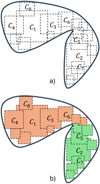 |
Fig. 1 Sketch of the void-finding procedure in an idealised 2D case. Top panel: complete set of volume-ordered cubes |

2.4 Void substructure
The capability to disentangle void substructure and finding voids-in-voids is a crucial feature for any void finder in both simulations and observations. AVISM can naturally tackle this problem by construction, as it is based on a hierarchy of nested grids at different levels of spatial resolution. This hierarchy starts from a coarse level, ℓmin, and reaches a given maximum level, ℓmax, with increasing resolution ∆xℓ/∆xℓ+1 = 2. The higher the level the better resolved are physical quantities and, therefore, their gradients and divergences become steeper as a result of the sharper reconstruction of density and velocity fields. Thus, by keeping the configurable parameters fixed, those regions that at lower levels of the grid hierarchy have smoother density gradients and velocity divergence and, therefore, satisfy the condition to belong to a void, are now split into several sub-voids at higher levels of refinement.
From an algorithmic point of view, in order to identify substructures correctly, an extra condition must be considered. When a cell is identified as a void centre candidate in a given level of refinement ℓ + 1, this cell can be immediately located within an already identified void at the lower level of refinement ℓ. The process of growing and merging the cubes at level ℓ + 1 is then restricted to occur inside the parent void defined at the lower level of refinement ℓ of the grid. An example of substructure identification is presented in Sect. 4.2.
3 Mock test
To justify the values adopted for the void thresholds in Table 1 and to assess the code robustness, we built a test that consists of a particle-only non-periodic snapshot of 107 particles in a L0 = 147.5 Mpc4 box at z = 0. Inside this box we built 50 ellipsoidal voids with a density profile as proposed by Ricciardelli et al. (2013) (note that this profile is a generalisation of the one presented by Colberg et al. 2005):
![Mathematical equation: $\rho \left( { < r} \right) = {\rho _e}{\left( {r/{R_e}} \right)^\alpha }\,\exp \left( {{{\left[ {r/{R_e}} \right]}^\beta } - 1} \right),$](/articles/aa/full_html/2025/12/aa54513-25/aa54513-25-eq16.png) (6)
(6)
with Re the void effective radius5, α = 0.07 and β = 1.32. These mock voids, which are not allowed to overlap, have a semimajor axis ranging from 12 to 50 Mpc. Following Sheth & Van De Weygaert (2004), the mean density contrast inside Re is set to δe = −0.8. We refer to Appendix A for more details on the construction of this test. The perfect elliptical shape of these voids represents a demanding challenge for AVISM, since its basic building blocks are cubes. However, the algorithm structure and the combination of multiple-sized cubes transform this apparent disadvantage into a powerful tool for describing complex void shapes.
This collection of idealised voids is a very stringent test as all void features are well-known and can be accurately computed. Thus, the comparison of different quantities estimated from the original sample (denoted by subindex T, standing for True) and from the counterparts produced by AVISM will shed light on the code’s behaviour. In this particular application, we used a 1283 cell grid, which results in a resolution of ~1 Mpc, and we set Nngh = 32 (the default value). For the sake of clarity, and in order to study the code’s performance depending on voids’ size, we segregated voids into three sizes: small (Re < 10 Mpc), intermediate (10 Mpc < Re < 17 Mpc), and large (Re > 17 Mpc).
Figure 2 displays clockwise the relative errors, defined as ∆X = |1 − X/XT|, for four quantities: the centre offset, the effective radius, the inverse porosity6, and the ellipticity7. The results for small, intermediate, and large voids are shown in blue, gold, and red, respectively.
As expected, the larger the void, the better the void finder is capable of reproducing the true values of its properties, since there are more resolution elements (grid cells) to catch the true shape. In contrast, in small voids, a single cell can be approximately 10 per cent of the effective radius, thus producing larger uncertainties in the void properties, especially in the size (effective radius) determination. Intermediate voids lie halfway between the other two behaviours, hence providing a smooth transition between the different accuracies.
Naively, one could think of using finer grids to overcome possible resolution effects, but depending on the data, this could worsen the situation. For instance, using a 5123 grid on the mock test input, many cells could be left without particles, leading to over-smoothed and noisy data after the interpolation process. On the contrary, increasing the number of particles always improves performance, as more numerical elements are used to sample the underlying density and velocity fields.
The resolution of the grid should also be chosen depending on the size of the volume under study and the application. When searching for voids at z ≈ 0, it could be counterproductive to resolve regions smaller than 1–2 Mpc, since this is the realm of galaxy clusters and filaments. Therefore, too high numerical resolution could lead to the creation of undesired boundaries that spuriously split voids. We consider a cell size of 1–2 Mpc a proper resolution to find large voids in the coarse level of resolution. When considering a hierarchy of nested grids with increasingly higher numerical resolution, as discussed earlier, the higher resolution captures steeper gradients that naturally divide voids into smaller parts, thus creating a structure of voids-in-voids.
In summary, AVISM is able to properly recover the 50 mock voids inside the analysed volume and correctly reproduce their main properties, especially for Re > 10 Mpc. Details on computational performance can be found in Sect. 5.
4 Application to cosmological simulations
After applying the new void finder to an idealised mock test, in this section we analyse the outputs from two complex cosmological simulations of a very different nature. In addition to studying different aspects of the performance of the code, we illustrate how AVISM can handle such different inputs.
In the first case, we used snapshots from amoving-mesh code (Lagrangian approach) in order to assess how the use of different numerical tracers, namely, dark matter particles, gas particles, dark matter haloes or galaxies, affect the void identification process. Moreover, this particular simulation uses a large number of dark matter and gas particles, thus emphasising the ability of the code to deal with a large number of numerical tracers. In a second application, we analysed a grid-based simulation (Eulerian approach) to show an example of substructure identification.
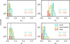 |
Fig. 2 Relative errors between the mock void sample and that obtained by AVISM as defined in the main text for four quantities: centre offset (top left), effective radius (top right), ellipticity (bottom left), and inverse porosity (bottom right). Colours denote the results for small (blue), intermediate (gold), and large (red) voids. The text within each panel displays the mean error of the quantity considered for each population. |
4.1 Numerical tracers
A crucial aspect underpinning the void-finding problem refers to the numerical elements used to define the physical quantities that, in turn, are used to identify voids. When analysing cosmo-logical simulations, different flavours of numerical tracers can be used: dark matter particles, gas particles (or cells), haloes, or galaxies. One might legitimately question how the chosen tracer affects the outcome of the void finder.
In order to demonstrate AVISM’s capabilities to handle different matter tracers, as well as their effect on the void identification, we ran the void finder on a z = 0 snapshot of the TNG300-2 cosmological simulation, from the IllustrisTNG suite (Nelson et al. 2019). This simulation models the evolution, from red-shift z = 127 to z = 0, of a cubic volume with 302.6 cMpc side length, containing 12503 gas and dark matter particles. It incorporates a comprehensive galaxy formation model that accurately tracks the formation and evolution of galaxies over cosmic time (Weinberger et al. 2016; Pillepich et al. 2018). The void finding algorithm has been applied with the default values described in Sect. 2.3 to four different tracers: all dark matter particles, all gas particles, all haloes and all galaxies. The results are shown in Fig. 3, where we display the distribution of voids inside a thin slice of 302.6 Mpc side length and ≈10 Mpc depth, together with the integrated density contrast field.
To provide a more intuitive comparison among the four void catalogues produced using the four different tracers, we used the Dice-Sørensen coefficient (DSC) (see Appendix C for details) as a metric to measure the degree of matching. We took the reference catalogue to be that produced by the dark matter haloes, as it represents a compromise in the number of numerical tracers. Voids in the other three catalogues that match with other voids from the reference catalogue with a DSC higher than 0.4 are displayed by a continuous contour line with the same colour. These are matches that have a high volume intersection. In the same manner, void matches that have a DSC value smaller than 0.4 are considered likely counterparts, although their intersected volume would be smaller. They are also drawn using the same colour but with dotted contour lines.
As a general trend, there is a reasonable match among the outcomes produced by the four different tracers. Nevertheless, the use of a larger number of numerical tracers leads to different spatial distributions of the physical quantities, with sharper features that would produce some voids in the reference catalogue to be split into smaller ones in the dark matter or gas particles catalogues. Along the same line, the fewer the number of tracer particles used, the smoother the density and velocity fields. This is the reason why the catalogue based on galaxies has the tendency to produce larger voids.
A more complete perspective is given by the VSF8 presented in Fig. 4, where the void catalogues produced by the four different numerical tracers are analysed. Two distinct behaviours are obtained: haloes and galaxies tend to yield larger voids, while dark matter and gas particles tend to produce smaller ones. These results reinforce the previously stated idea that the number of considered numerical tracers directly impacts the level of detected substructure.
A remarkable result is the fact that, although voids sizes and locations can vary to some extent, statistically, the results produced by the algorithm present an outstanding robustness against huge variations in the number of numerical tracers (~109 for gas or dark matter particles and ~106 for haloes or galaxies).
4.2 Substructure identification
To provide an example displaying the outcome of our substructure approach, we applied AVISM on a snapshot at z ≈ 0 from a simulation produced by the MASCLET hydrodynamic and N-body code (Quilis 2004), which is based on an AMR scheme. This simulation describes the evolution of a 100 cMpc/h cosmological box using nine levels of refinement, which allows a peak spatial resolution of 1.1 ckpc. It is similar to the one described and applied in Ricciardelli et al. (2013) to study void structures, but has better spatial resolution. The grid refining criteria were chosen to ensure a proper description of the physical quantities in void regions and, hence, to obtain a proper evolution of these structures in the simulated volume.
Regarding the void-finding methodology, the values for the thresholds used to obtain these results correspond to the default configuration. In addition, in this case, the void finder was run with a three-level grid hierarchy (ℓ = 0, 1, 2) from which substructure can be studied in detail. Fig. 5 shows a slice of 5 cMpc depth zooming in on a Re ≈ 40 Mpc void at ℓ = 0 (solid dark blue line) together with its largest sub-void at ℓ = 1 (dash-dotted light blue line) and a substructure of that sub-void at ℓ = 2 (dashed white line). Note that, in order for the illustration to be clear, we are only showing a void at each level of the hierarchy, but more substructures were obtained for the ℓ = 0 void in the other two levels. As explained above, the same thresholds were applied for the three different resolutions. At ℓ = 0 (lowest resolution), the physical quantities are smooth, and neither the velocity divergence nor the density gradient presents substantial variations in space, thereby resulting in larger voids. For ℓ > 0, the increase in resolution makes the divergences and gradients steeper. Consequently, more cells exceed the thresholds to stop void growth, yielding a set of smaller voids that are contained inside the larger ones at lower levels of the hierarchy and can be understood as physical substructures. Let us draw attention to how less dense filaments and tendrils become the boundaries of the sub-voids at higher levels of refinement.
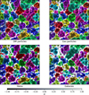 |
Fig. 3 Distribution of voids obtained by AVISM when applied to a z = 0 snapshot of the TNG300-2 simulation on four different matter tracers: dark matter particles, gas particles, haloes and galaxies. The images show, for each tracer, all voids intersecting a thin slice of 302.6 Mpc side and ≈10 Mpc depth, together with the integrated density field, for which a colour bar is displayed. Voids matching those from the reference catalogue (using haloes as matter tracers) with a DSC coefficient larger (smaller) than 0.4 are displayed using the same colour and continuous (dotted) lines. |
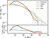 |
Fig. 4 Top panel: VSF for the different void catalogues obtained by AVISM when run on four different numerical tracers of the TNG300-2 cosmological simulation from the IllustrisTNG suite. Bottom panel: relative difference with respect to the reference VSF obtained using haloes as tracers. |
5 Computational performance
To evaluate the code’s computational performance, we applied AVISM to the mock test volume described in Sect. 3 using different grid and CPU configurations. In addition, in order to assess the particle-to-grid interpolation scalability, we also produced different versions of the test varying the number of particles. The code was compiled by the GNU Fortran 11.4 compiler and was run on an AMD Ryzen Threadripper PRO 3995WX (64 cores) CPU.
Building a k-d tree implies an initial cost of O(Npart log Npart) (Bentley 1975), with Npart the number of input particles. Then, searching for the neighbours around some point, implies a O(log Npart) complexity. Hence, when using a grid consisting of Ncell cells, the particle interpolation process scales as O(Ncell log Npart) for the velocity, and as O(Npart log Npart) for the density.
Regarding the void-finding algorithm (see Sect. 2), it requires the creation of a set of cubes covering all regions susceptible to belonging to a void. To achieve this, it loops over all cells belonging to the grid, growing a cube where the corresponding physical thresholds are fulfilled. Thus, since not every cell has to be expanded (not every cell fulfils the necessary physical thresholds), and many will already be part of a cube, we expect the algorithm to have, at maximum, a O(Ncell) complexity. Once all cubes are created, they are merged depending on whether they overlap or touch each other, leading to a complexity of  , with NC the total number of cubes. Nevertheless, we leveraged our particular implementation of the k-d tree algorithm, allowing us to accelerate the process by restricting the merging procedure to cubes that are within a certain distance. Time complexity thus becomes O(NC log NC), but, since NC ∝ Ncell, the merging process ultimately has a O(Ncell log Ncell) complexity, at most. On the other hand, as explained in Sect. 2.3, the final step is to get rid of possible holes in the final void structures by applying the BFS method, which presents O(Ncell) scaling.
The volume of the region we want to analyse, either from simulations or observations, is also a key ingredient affecting the performance of the void finder. As the Universe’s volume is mostly occupied by voids, the number of these structures increases with the volume of the considered region. Additionally, the number of non-void structures, such as clusters, filaments and sheets, also increases, making the process of identifying the cells in voids, creating cubes, and merging them to produce the final voids more costly.
To check the time complexity in AVISM, we performed two different sets of runs of the mock test presented in Sect. 3. In the first, we fixed the number of particles to Npart = 107 and varied the grid number of cells from 643 to 5123 in powers of 23. Then, we performed a second test fixing the grid to 1283 and varied the number of particles from 106 to 109 in powers of 10. Both tests were run using 16 CPU cores. The results can be found in Fig. 6. The top panel shows how the wall time scales as O(Ncell) at maximum, better than previous expectations. Regarding the number of particles, the bottom panel also exhibits a closer time complexity to the expected O(Npart log Npart).
Regarding the code scalability when running on parallel systems, the speed-up of the current version is good, although some parts of the code cannot be parallelised and, therefore, result in bottlenecks holding the scalability. The void expansion and merging processes present some problematic race conditions, and most parts of these code sections have to be run serially. Nevertheless, the particle-to-grid interpolation (including k-d tree construction) which represents, depending on the run, the most computationally expensive part, can be perfectly parallelised by means of OpenMP directives. The speed-up for the mock test described in Sect. 3, using a single grid level ℓ = 0 of 2563 cells and 107 particles, is presented in Fig. 7. The computational time decreases significantly up to 32–64 cores, after which the speed-up starts to flatten out. Indeed, this scaling occurs due to the fact that an increasing number of threads cannot reduce the computational cost of the void-finding and merging processes, as these are run serially. This figure shows a balanced case in which the number of particles and cells are within a similar order of magnitude (~107). In unbalanced cases the situation can get better (worse) if the number of particles is significantly greater (lower) than the number of cells in the grid.
Let us stress one final feature of AVISM regarding its computational performance. The code can handle - both in terms of memory and CPU time – very large volume datasets in an extremely efficient way. To highlight this point with a specific example, the TNG300-2 simulation snapshot at z = 0 was analysed using all dark matter particles (12503) with the default set of parameters described in Sect. 2.3. Running the code with 32 cores took 1 hour and 10 minutes and allocated a maximum of ~360 GB of RAM at its consumption peak.
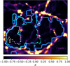 |
Fig. 5 Slice of a zoom-in on a region centred at a Re ≈ 40 Mpc void at ℓ = 0 (solid dark blue line), together with its largest sub-void at ℓ = 1 (dash-dotted light blue line), and a substructure of that sub-void at ℓ = 2 (dashed white line). The slice is 5 Mpc in depth. The colour palette displays the integrated density contrast. The analysis was performed on a snapshot of a MASCLET simulation at z = 0. Additional substructures were obtained for the same void and its sub-voids; however, only one of each level is shown for the sake of clarity. |
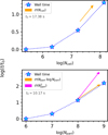 |
Fig. 6 Code time complexity. Times are normalised with respect to t0, the wall time for the minimum number of cells or particles considered in this test, shown below both panel legends. Top panel: wall time against the number of cells. Bottom panel: wall time against the number of particles interpolated onto the grid. In yellow and purple, different time complexities are given as a reference. Logarithms are taken in base 10. |
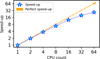 |
Fig. 7 AVISM’s speed-up against the number of CPU cores used. In yellow, a perfect speed-up is given as a reference. |
6 Comparison with DIVE and ZOBOV
Every algorithm has its own strengths and caveats, and therefore, when describing a new computational tool, it is crucial to contextualise its performance by comparing it with some of the codes widely used by the community. In this sense, it is of utmost importance to compare AVISM with some of the most popular void finders. To carry out this comparison, we considered two well-known and widely used codes, each of them broadly representing the two most common approaches used in the void-finding algorithms:
DIVE (Zhao et al. 2016): Delaunay trIangulation Void findEr is a C++ tool for identifying all empty spheres that are constrained by four elements of a point set, using the Delaunay triangulation (DT) technique. It is able to resolve all the maximal spheres that are empty of whatever element that is used as a tracer, such as galaxies in either a real survey volume or a periodic simulation box. These spheres are regarded as a special type of cosmic voids (DT voids), which are allowed to overlap with each other. The output of the code are the spatial positions of the centres of these spheres, along with their radii. However, these spheres are not actual voids but rather candidates for being voids, since overlaps must be eliminated to obtain a set of disjoint voids. Although DIVE was conceived for finding large-scale underdensities in the very diluted sample of luminous red galaxies (LRGs), not for studying void structure and dynamics, it has been widely used recently (Contarini et al. 2022; Tamone et al. 2023; Fernández-García, Elena et al. 2025) to study void statistics and constrain cosmological parameters. Caution must be taken, however, when comparing it with other void finders due to its particular approach. With this in mind, our goal is to compare AVISM’s voids with those of DIVE on a simple void-placement and size basis.
VIDE (ZOBOV) (Sutter et al. 2015): Void IDentification and Examination toolkit is an open-source Python/C++ code for finding cosmic voids in galaxy redshift surveys and N-body simulations. It is built on ZOBOV (Neyrinck 2008), which builds a Voronoi tessellation of the tracer particle population and utilises the watershed transform to group Voronoi cells into zones, eventually identifying voids. VIDE has several modifications and improvements with respect to ZOBOV, both in terms of computational performance and the algorithm’s design. The outcome of this void finder is extensive. We focus on the void volume, particles belonging to each void and volume occupied by each particle’s Voronoi cell. This void finder targets the same goals as AVISM, namely the study of the full void structures and substructures across cosmic time in simulated and real data. In order to make the comparison clearer, we focus on void placement and sizing, such as in the case of DIVE. Moreover, throughout the rest of the paper, we refer to VIDE as ZOBOV, for the sake of clarity.
In order to compare the performance of AVISM with that of DIVE and ZOBOV, we applied the three void finders to the same simulation output. For the sake of a complete comparison, the simulation must satisfy the following requirements:
It is publicly available, for the sake of reproducibility.
It describes a large cosmological volume (L0 ≳ 400 Mpc), thus containing sufficient void statistics.
It already has an available halo catalogue to which we can apply the void finders.
The comparison was carried out using a halo catalogue as an input, first, because it is generally faster for all void finders since there are fewer tracers to process and, second, because DIVE is particularly designed for this type of input or survey data (low density of tracers). A suitable simulation fulfilling all of these requirements is mini-UCHUU, from the UCHUU N-body simulations suite (Ishiyama et al. 2021)9. It uses Planck cosmology (Planck Collaboration VI 2020) with Ωm = 0.3089, h = 0.6774, σ8 = 0.8159 and ns = 0.9667 with a cosmological box of L0 = 400 Mpc/h ≈ 591 Mpc at z = 0 containing 25603 particles with a softening length of ε = 4.27 Mpc/h. All simulation outputs have already been analysed by means of the ROCKSTAR halo finder (Behroozi et al. 2012). We are interested in the last output (z = 0), where there are Nh ≈ 1.7 × 10⁷ haloes with Mvir > 1010 M⊙. While DIVE only requires the position of each tracer, ZOBOV also needs mass and AVISM needs positions, velocities, and masses. Moreover, the DIVE and ZOBOV inputs were reduced in order to accommodate the number of tracers to the requirements of each code. The outcome of the void-finding processes for these algorithms, unlike AVISM, strongly depends on the density of tracers (e.g. see Massara et al. 2022). Hence, we properly chose this quantity in order for the void finders to produce void samples with good statistical properties (Sutter et al. 2014). Thus, following the analysis performed in Zhao et al. (2016) and the approach considered in Fernández-García, Elena et al. (2025), we only used haloes above Mvir > 1013 M⊙ in order to achieve a tracer density of  for the DIVE case. Regarding ZOBOV, using a mass cut of Mvir > 1012 M⊙ we obtain a tracer density of
  . Hence, to perform as fair a comparison as possible, DIVE and ZOBOV were applied to a subset of the provided input, whereas AVISM was run on the whole input, using a single-level grid (substructure was ignored in this comparison) of 2563 cells together with the default thresholds described in Sect. 2.3.
Figure 8 presents the outcome of the different void finders applied to the mini-UCHUU haloes catalogue at z = 0. In the top panel, the VSF is presented together with 2σ of the Poisson shot noise error for the AVISM case. Next, in the middle panel, we find the cumulative VSF with the same error and a (best) theoretical fit following the model developed in Sheth & Van De Weygaert (2004) (henceforward, the SvdW model) and further expanded in Jennings et al. (2013) (Vdn model), where the excursion-set formalism is used and voids are treated as spherical regions around density minima. In Appendix B, we provide a brief summary of the basic concepts and considerations used to compute the fit. In the bottom panel, we present the cumulative volume filling fraction as a function of radius. This last plot describes how much volume is occupied by voids larger than a given effective radius.
AVISM and ZOBOV display similar behaviours in the size function, both in the cumulative and differential representations, with the second finding significantly fewer small voids. DIVE has the largest void population with 3230 voids found, but it is shifted towards small sizes. None of the algorithms is able to closely follow the theoretical fit; however, AVISM and ZOBOV show a consistent trend with it for Re ≳ 15 Mpc within 2σ of the Poisson error. The deviation from the theoretical fit is mostly due to the arbitrary shapes voids can have (except for the DIVE case), which hugely differ from those assumed in the spherical formalism (see Appendix B for more details). Moreover, the mean density contrast inside voids varies in each case and can significantly deviate from δ = −0.8, thereby again violating the conditions under which the SvdW formalism is applied. Overall, the three algorithms approximately converge in terms of volume filling fraction, with AVISM maximising the covering (63%). This result indicates that the three algorithms are able to detect the same total volume in voids, whereas this total volume is distributed in void catalogues with different ranges of sizes and shapes.
For the sake of a visual comparison, Fig. 9 displays a thin slice through the centre of the box, showing those voids intersecting the considered slice as found by each method. Voids are presented overlaying the projected contrast density field as interpolated by AVISM. Furthermore, so as to get a more detailed visual inspection of the three samples, we matched the individual voids produced by the three codes inside the slice (not the entire input box) by using the DSC coefficient defined in Appendix C as a metric to measure the similarity of voids. In a similar manner, as in Sect. 4.1, and taking AVISM result as the reference one, voids in the middle and bottom panels in Fig. 9 matching a void from this reference catalogue with a DSC value larger than 0.4 are displayed with a continuous line with the same colour as in the top panel. Similarly, counterparts with a DSC rate smaller than 0.4 are plotted with the same colour but using dotted lines, indicating a lower agreement. The three algorithms successfully identify most major voids in the intersecting slice. However, a region classified as a single void by one method may be divided into two distinct regions by another. Additionally, in some cases, a zone where one algorithm fails to detect a void is successfully identified by another. Hence, although they are statistically similar, ZOBOV and AVISM can find different void shapes, sizes, and centres. It is also interesting how the centres and sizes found by DIVE and AVISM coincide in many cases, in spite of having such divergent methodologies to identify voids.
To get a more quantitative comparison among finders, we then calculated the DSC (see Appendix C) of all voids inside AVISM’s catalogue against the other two. This time, the cross-match was carried out with all voids inside the input box, and duplicates were not allowed; that is, a match could not be shared by two different voids from the same catalogue. Figure 10 displays the cross-match between AVISM’s voids and those found by DIVE and ZOBOV, displaying the radius identified by the void finders against each other together with the colour-coded DSC corresponding to each match. The small panels below the main ones show, at each radius, the fraction of voids that match with a DSC exceeding a certain value given by the colour palette. Redder (bluer) colours display higher (lower) agreement between the void finders. The dashed black line shows the ideal case where voids matched among the void finders have the same effective radius, whilst the dotted line displays a linear fit to the R − R relation, weighted by the DSC values. Strikingly, despite their very different natures, AVISM and DIVE display the best agreement when considering the volume intersection. Indeed, the fraction of AVISM voids intersecting with DIVE voids with a DSC above 0.4 ranges from ≈40% to ≈70% for Re ≳ 20 Mpc. Also, a non-negligible fraction of 10–20% voids with an overlapping index above 0.6 can be found, especially for the middle-sized part. This indicates that the two methodologies, to some extent, place voids in similar places with alike volumes. Regarding sizes, although the scatter is considerable, it is lower than the AVISM versus ZOBOV case; nevertheless, the RAVISM versus RDIVE fit significantly deviates from the 1:1 relation. This can be explained by the fact that DIVE finds, in general, smaller voids than AVISM.
The comparison of AVISM and ZOBOV voids shows greater scatter when it comes to the size-to-size correlation, although the RAVISM versus RZOBOV fit almost lies on top of the ideal 1:1 correspondence, since the two approaches yield a similar size distribution. The DSCs are generally worse than the cross-match of AVISM and DIVE catalogues. For Re ≳ 20 Mpc, the fraction of voids intersecting with a DSC above 0.4 ranges from 30% to 50%, approximately, with some matches fulfilling DSC > 0.6 at large radii. One would expect AVISM and ZOBOV to have a better match, as they both allow arbitrary void shapes and yield a similar VSF. A plausible explanation for this divergence is their dissimilar definitions of voids, which, especially for the smaller ones, can return them in very different places and sizes. In fact, as can be seen in Fig. 9, while ZOBOV identifies voids that are excluded by AVISM due to their high densities, it struggles to find voids in very underdense regions, possibly due to the small number of particles (numerical tracers), whereas the other two void finders successfully identify them.
For the sake of completeness, Fig. 11 provides a cross-match of the ZOBOV and DIVE void catalogues. From all the comparisons, this is the best in terms of raw matching, as 97% of ZOBOV’s voids are matched by DIVE’s. Nevertheless, the quality of these is not as high as the AVISM versus DIVE case: the fraction of voids intersecting with DSC above 0.6 is never higher than 5–10%, and those intersecting with DSC > 0.4 are never higher than a ≈50% fraction. Concerning sizes, a similar correlation to the RDIVE versus RAVISM fit is obtained, with similar scatter and slope. This is, again, due to the fact that DIVE’s voids are smaller than those identified by the other two approaches.
Finally, it can be seen that, in all the comparisons we carried out, the agreement between the void finders maximises at larger void sizes and starts to decline at smaller radii. This can be explained by the fact that, unlike the large ones, small voids are hugely affected by Poisson noise, as the number of resolution elements defining them is poor and, thus, little changes in the sampling or methodology can yield very different results (e.g. centre placement and size).
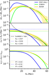 |
Fig. 8 Statistical comparison of the void distribution, as found by DIVE (blue), ZOBOV (green), and AVISM (yellow) using the mini-UCHUU haloes catalogue at z = 0 as input. Top panel: VSF. The gold-shaded region represents 2σ of the Poisson shot noise error. Middle panel: cumulative VSF with horizontal lines depicting the total void number density and the corresponding total void count (NV). The dashed black line represents the best match for the theoretical SvdW+Vdn model (Sheth & Van De Weygaert 2004; Jennings et al. 2013). Bottom panel: volume filling fraction of voids above a given radius. Horizontal lines depict the total filling fraction (FF). |
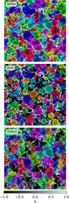 |
Fig. 9 Distribution of voids intersecting a thin slice of 400 Mpc/h side length through the centre of the box. Top, middle, and bottom panels show, respectively, results from AVISM, DIVE, and ZOBOV. Different colours are used to show void zones. Voids matching those from the reference catalogue (AVISM in this case) with a DSC coefficient larger (smaller) than 0.4 are displayed using the same colour and continuous (dotted) lines. Voids are shown overlaid on the integrated contrast density field as interpolated by AVISM, represented in a grey colour scale with values displayed in the colour bar below. |
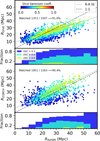 |
Fig. 10 Cross-match between AVISM’s voids and those found by DIVE (top panel) and ZOBOV (bottom panel). For all AVISM voids, a point is drawn with the best match found in the other catalogues displaying, first, the colour-coded Dice-Sørensen coefficient for the match and, second, the radius of the corresponding counterpart on the vertical axis. The dashed black line shows the ideal case where the voids matched among the void finders have the same effective radius, whilst the dotted line displays a linear fit to the R − R relation, weighted by the DSC values. The small panels below each main panel show the fraction of voids for each radius that are matched with a DSC above a certain value, given by the different colours displayed in the palette. Redder (bluer) colours indicate higher (lower) DSC, meaning that the matched voids are more similar (different). |
7 Application to survey data
One of the main goals of this project is to design a void finder algorithm that can be applied either to cosmological simulation outputs or to real survey data. While the use of the void finder can be straightforward in the first case, as the density and velocity fields are generally known, the situation could be more complex in the latter case. In this section, we discuss how these fields could be estimated in order for AVISM to be applied to galaxy catalogue surveys.
The estimation of the density and velocity fields requires careful treatment due to inherent problems such as sample completeness, galaxy bias, or RSDs. Therefore, the problem of reconstructing such fields in galaxy surveys is an open, tough issue that involves the work of many groups nowadays. Thus, for AVISM to be successfully applied to observational data, it is necessary to transform the raw galaxy distribution into the density and velocity fields evaluated onto a cubic grid, considering all the pertinent corrections. Especially important is the case of the velocity field, whose use to identify voids is a distinguishing feature of AVISM. As a consequence of this, the application of AVISM to observational data requires a pre-processing step, and the use of complementary tools to reconstruct the density and velocity fields is compulsory. The capabilities of such field reconstruction procedures are crucial for the void finder’s performance.
A first approach would be to create a continuous density field using the galaxies as mass particles, conveniently smoothed onto a grid, and corrected for completeness, bias, and RSDs. Later, the use of the linear approximation (Eq. (4)) would provide us with the velocity divergence. This would be a misleading strategy, as no new information would be introduced besides the one provided by the density field, and, therefore, the velocity divergence condition would be superfluous.
As previously mentioned, the reconstruction of the density and velocity fields associated with observational data beyond the linear regime is an extremely difficult task. Nevertheless, several options have recently produced huge advances in the topic. Let us describe briefly some of these new options. The first one is the approach based on Bayesian inference frameworks such as BORG (Jasche & Lavaux 2019) or COSMIC BIRTH (Kitaura et al. 2021). These methods hinge on the basic idea of producing constrained initial conditions that, when conveniently evolved in a suite of numerical simulations, yield matter distributions at z ~ 0 compatible with the observational data considered. Thus, non-linear density and velocity fields are obtained. The second family of methods uses neural networks (NNs) that have been trained working with several simulation datasets. Once the NNs are trained, they are properly fed with the observational data, giving the non-linear density and velocity fields as the output (Wu et al. 2021; Lilow et al. 2024).
We applied AVISM to the 2M++ survey (Lavaux & Hudson 2011), which is a superset of the all-sky 2MRS survey (Huchra et al. 2012). We used two methods to reconstruct the density and velocity fields. The first one uses the methodology described in Carrick et al. (2015)10 to produce a linear estimate of those fields. Therefore, as discussed before, this approach does not introduce additional information concerning the velocity field beyond what is given by the density reconstruction. A similar approach is the one used by the CORAS code (COnstrained Realisations from All-sky Surveys; Lilow & Nusser 2021) to analyse the 2MRS survey. The second method uses data from Manticore-Local (McAlpine et al. 2025), where a suite of N-body simulations were carried out starting from constrained initial conditions produced by the BORG code (Jasche & Lavaux 2019) compatible with the data from the 2M++ galaxy survey. This methodology allows for obtaining a set of realisations with the fully non-linear density and velocity fields. The void finder was applied to the averaged fields, considering the whole suite of realisations.
The outcome of this test are two all-sky void catalogues within a radius of 200 Mpc/h. Figure 12 shows two slices through the centre of the survey with all voids intersecting it as found by AVISM when supplied with the non-linear reconstructed density and velocity fields given by Manticore-Local (left panel) and the linear fields obtained by Carrick et al. (2015) (right panel), respectively. To compare the two catalogues obtained, we performed a similar comparison as in Sect. 6 with the different void finders. We cross-matched the two 2M++ catalogues to quantify the extent to which the samples correlate. We find that 33% of voids agree with a DSC above 0.4 while only 12% show a DSC above 0.6. This means that the non-linear features introduced in the McAlpine et al. (2025) realisations, which are not present in the Carrick et al. (2015) linear reconstructions, play an essential role in order for AVISM to properly identify voids. The linear reconstruction was downgraded to ensure the same spatial resolution than in the Manticore-Local data, which is ≈3.9 Mpc. The two void catalogues were obtained using the same set of thresholds and parameters in AVISM.
Let us note that, although errors in the velocity field can be high, their impact is not critical for AVISM, since voids are identified (by default) under the assumption that they are expanding regions with positive velocity divergence. That is, AVISM is only concerned with the sign of the divergence, as negative divergence indicates non-void regions. This is a crucial feature of our void finder that mitigates the impact of large errors in the velocity divergence, allowing it to reasonably recover the distributions of voids with their complex 3D shapes as long as the velocity divergence sign is correct.
We wish to clearly state that in the case of observational data not pre-processed to provide either density or velocity information, AVISM cannot be directly applied and must instead collaborate with an external tool capable of reconstructing the required fields. However, rather than being a limitation, this represents a new opportunity for collaboration and integration with the aforementioned tools.
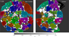 |
Fig. 12 Slice through the centre of the 2M++ galaxy survey with all voids intersecting it as identified by AVISM when applied to the McAlpine et al. (2025) (non-linear) and Carrick et al. (2015) (linear) density and velocity reconstructions. We use the supergalactic coordinate system (SGX, SGY, and SGZ) defined by De Vaucouleurs et al. (1991). The slice is ≈8 Mpc deep and contains the supergalactic plane (SGZ = 0). The void-finding procedure was restricted to the inner R ≤ 200/h Mpc in both cases. Near cosmological structures are highlighted with capital letters: the Virgo (V), Hydra-Centaurus (H), Norma (N), Shapley (S), and Perseus (P) clusters together with the Sculptor (S), Hercules (H), and Boötes (B) voids (Tully et al. 2019). Voids from the linear catalogue matching that from the non-linear with DSC coefficients larger (smaller) than 0.4 are displayed using the same colour and continuous (dotted) lines. The grey scale displays integrated density contrast. |
8 Summary and conclusions
In this paper, we presented AVISM, a novel void finder algorithm designed to identify cosmic voids within LSS datasets. The algorithm was thoroughly tested and validated across a wide range of scenarios, including mock void catalogues, the full output of the TNG300-2 cosmological simulation (dark matter, gas, haloes, and galaxies), a dark matter halo catalogue from the mini-UCHUU simulation, and real galaxy survey data. Moreover, an extensive comparison was carried out with two other state-of-the-art void identification algorithms, namely the DIVE and ZOBOV codes. Our results demonstrate the robustness and versatility of the method in identifying voids within the LSS of the Universe, providing valuable insights into their distribution and properties.
AVISM’s performance was also rigorously evaluated in terms of computational efficiency and scalability. We tested its behaviour with varying input sizes, including the number of particles and the resolution of the auxiliary grid, and analysed its CPU scaling and efficiency. These tests confirm that the algorithm is capable of handling efficiently large datasets, both in terms of memory management and wall time, making it a practical tool for analysing current and future cosmological data, including simulation outputs such as dark matter haloes and particle information, as well as observational data from galaxy surveys.
The idea underpinning AVISM is that voids are expanding, low-density, large structures. Here, we provide a summary of its methodology, performance, and applications:
1. AVlSM’s void-finding methodology. The code finds voids by means of a uniform auxiliary grid, in which density gradients and velocity divergences are computed. It is able to handle both Eulerian and Lagrangian data. In the first case, the creation of the auxiliary grid is straightforward, as it uses the original data structure. In the second one, continuous density and velocity fields are computed on the grid by means of an interpolation method similar to the SPH approach. When the original data do not include velocities (a common situation in observational data), several strategies are outlined to address this issue. Although information on velocities is required to compute velocity divergences, the accuracy of velocity reconstruction is a minor issue as long as the correct sign and ordering of the velocity divergence is caught. With density contrast and peculiar velocity divergence computed on the auxiliary grid, these quantities are used, first, to label cells as candidates for void centres when they satisfy two basic conditions (δ < δ1 and ∇ ⋅ v > ∇ ⋅ vth) and, later, to expand them under some conditions. In the end, this process yields a set of cubes  covering all regions susceptible to being part of a void.
After a volume-ordered merging process, a set of unstructured non-overlapping simply connected voids  is obtained. The previously described procedure can be repeated using a set of finer nested grids with higher spatial resolution. In this manner, a whole hierarchy of voids-in-voids and a deep insight into the voids’ substructure can be easily achieved.
2. Tests and computational performance. We ran AVISM on a mock test where a set of idealised voids were located. The exact properties of this void collection are completely known. The void finder recovered most quantities with errors ranging between 1% and 20%, depending strongly on void sizes. Smaller voids are described with fewer numerical resolution elements and thus exhibit higher errors.
To test the versatility and robustness of the algorithm, we applied AVISM on the full output of the TNG300-2 simulation from the IllustrisTNG suite, using dark matter and gas particles, dark matter haloes, and galaxies as different numerical tracers. Although most voids are well identified by running the void finder on the different matter tracers, and several voids are identified as the same by the four runs, noticeable differences arise in the void spatial distribution. These differences stem from variations in the density and velocity fields used to obtain the voids, due to differences in number density, positions, and masses of the tracers involved. Despite this, the size distribution, and hence the void statistics, seems to be robust against large variations in the number of numerical tracers used to reconstruct the density and velocity fields (from 106 to 109)11.
Regarding computational performance, the algorithm displays O(Ncell) and O(Npart log Npart) time complexities, thus scaling well both in grid resolution and number of input particles. The code is written in Fortran 2008 and is parallelised using OpenMP. However, due to the structure of some parts, the speed-up when running the code in more than approximately 32 threads is poor. This issue will be improved in future versions.
3. Code comparisons. We carried out a thorough comparison between AVISM and two other state-of-the-art void finder algorithms, namely DIVE (Zhao et al. 2016) and ZOBOV (Neyrinck 2008; Sutter et al. 2015). We applied the three algorithms on the same input, consisting of a z = 0 snapshot from the mini-UCHUU N-body simulation (Ishiyama et al. 2021), for which a dark matter halo catalogue already exists.
Due to their unstructured void-finding behaviours, AVISM and ZOBOV display similar patterns in VSF, with the former identifying a larger population of voids at smaller radii. The spherical void finder DIVE obtains a void sample shifted towards smaller sizes.
When examining the one-by-one match between the three codes, AVISM and DIVE exhibit the best agreement in terms of volume overlap, as their matches have the highest DSC values. In contrast, the comparison between AVISM and ZOBOV yields lower overlap, indicating a lower level of agreement between these two algorithms. However, the size correlation cross-match between AVISM and ZOBOV voids is closer to the ideal match trend (1:1), reflecting the similarity in their void size distribution. For completeness, a comparison between DIVE and ZOBOV was also carried out, with the agreement lying between that of the other two comparisons.
As a general conclusion, the three algorithms are somehow able to find similar statistical properties despite their different natures. However, although correlated, they identify different void populations (placed in different regions), since only a small fraction of voids (20% at most) have a good agreement in terms of volume overlap (DSC > 0.6).
4. Application to real observational data. AVISM can be used to search for voids in galaxy surveys. The code can internally compute the density field from a particle-like input provided by the user, which includes the position and mass of each galaxy, and the velocity divergence is calculated using linear theory. In this case, the velocity divergence condition does not introduce any additional information beyond the density field, leading to results that do not take advantage of the full potentialities of the code. Nevertheless, in this type of application, it is strongly recommended to pre-process the survey data with complementary external tools such as those described in Lilow et al. (2024) or McAlpine et al. (2025), which are able to produce cubic grids with the non-linear density and velocity fields. As a demonstration, we identified voids within the 2M++ survey (Lavaux & Hudson 2011) using data from a linear reconstruction of the density and velocity fields given by Carrick et al. (2015) and the non-linear Manticore-Local (McAlpine et al. 2025) output as inputs for AVISM. We provide two slices aligned with the supergalactic plane (Fig. 12), with all voids intersecting it.
AVISM is a public tool that can be widely used, both on simulated and observed data. A brief summary of its strengths that justify its application to future datasets is the following:
The code defines voids as expanding, low-density regions, and it uses geometrical and dynamical information to search for them;
The code can handle raw simulation outputs, halo catalogues, and galaxy surveys, taking into account periodic boundary conditions if the user requires it;
No prior assumption about the void shapes is made, allowing for a full 3D description of these regions;
Large volumes of data can be treated (i.e. more than 1010 particles) due to the code’s parallelisation and optimised time complexity;
The outcome of the void finder strongly depends on grid resolution but weakly on numerical tracer density (e.g. galaxies and dark matter haloes), as particle data are interpolated onto an auxiliary grid. This sets our method apart from other existing tools;
Although the voids found by this approach are unstructured, the complete 3D shape is defined on the auxiliary grid. This allows the user to easily distinguish which region belongs to each void and permits an easy and fast search of galaxies within voids, such as in spherical void finders;
The void-finding process can be applied at different levels of resolution using finer grids, leading to a list of voids-in-voids.
In conclusion, the void finder implementation presented in this work is a fast, robust, and versatile choice for studying voids in the context of the LSS of the Universe. Its ability to accurately and efficiently identify voids across diverse datasets makes it a powerful tool for cosmological research. Future work will focus on further expanding and optimising the algorithm, exploring its application to larger and more complex datasets, as well as leveraging its results to shed light on problems such as the characterisation of galaxies in voids or the constraints on cosmological parameters.
We refer to Sect. 2, where the GitHub repository link can be found. In this public repository, we provide the user with the code’s documentation, basic tools for handling simulation outputs such as the Mini-UCHUU halo catalogue analysed in Sect. 6 or the TNG300-2 simulation particles, raw galaxy survey data, and reconstructed grids (see Sect. 7), in order to provide proper input for the void finder. A Python reader for AVISM’s output is also provided.
Acknowledgements
We thank the anonymous referee for the valuable insight and constructive comments that helped improving the quality of this manuscript. We thank S. McAlpine and collaborators for providing us with the Manticore-Local data. This work has been supported by the Agencia Estatal de Investigación Española (AEI; grant PID2022-138855NB-C33), by the Ministerio de Ciencia e Innovación (MCIN) within the Plan de Recuperación, Transformación y Resiliencia del Gobierno de España through the project ASFAE/2022/001, with funding from European Union NextGenerationEU (PRTR-C17.I1), and by the Generalitat Valenciana (grant PROMETEO CIPROM/2022/49). OM and DV acknowledge support from Universitat de València through Atracció de Talent fellowships. Simulations have been carried out using the supercomputer Lluís Vives at the Servei d’Informàtica of the Universitat de Valencia. We thank Institute de Astrofisica de Andalucia (IAA-CSIC), Centro de Supercomputacion de Galicia (CESGA) and the Spanish academic and research network (RedIRIS) in Spain for hosting Uchuu DR1, DR2 and DR3 in the Skies & Universes site for cosmological simulations. The Uchuu simulations were carried out on Aterui II supercomputer at Center for Computational Astrophysics, CfCA, of National Astronomical Observatory of Japan, and the K computer at the RIKEN Advanced Institute for Computational Science. The Uchuu Data Releases efforts have made use of the skun@IAARedIRIS and skun6@IAA computer facilities managed by the IAA-CSIC in Spain (MICINN EU-Feder grant EQC2018004366P). This research has made use of the following open-source packages: NumPy (Harris et al. 2020), SciPy (Virtanen et al. 2020), Matplotlib (Hunter 2007), and CAMB (Lewis & Challinor 2011).
References
- Aragon-Calvo, M., & Szalay, A. 2013, MNRAS, 428, 3409 [NASA ADS] [CrossRef] [Google Scholar]
- Argudo-Fernández, M., Hernandez, C. G., Verley, S., et al. 2024, A&A, 692, A258 [NASA ADS] [CrossRef] [EDP Sciences] [Google Scholar]
- Behroozi, P. S., Wechsler, R. H., & Wu, H.-Y. 2012, ApJ, 762, 109 [Google Scholar]
- Bentley, J. L. 1975, CACM, 18, 509 [Google Scholar]
- Bernardeau, F., & van de Weygaert, R. 1996, MNRAS, 279, 693 [Google Scholar]
- Bond, J., Cole, S., Efstathiou, G., & Kaiser, N. 1991, ApJ, 379, 440 [NASA ADS] [CrossRef] [Google Scholar]
- Bos, E. P., van de Weygaert, R., Dolag, K., & Pettorino, V. 2012, MNRAS, 426, 440 [NASA ADS] [CrossRef] [Google Scholar]
- Carrick, J., Turnbull, S. J., Lavaux, G., & Hudson, M. J. 2015, MNRAS, 450, 317 [Google Scholar]
- Cautun, M., Van De Weygaert, R., Jones, B. J., & Frenk, C. S. 2014, MNRAS, 441, 2923 [CrossRef] [Google Scholar]
- Cautun, M., Paillas, E., Cai, Y.-C., et al. 2018, MNRAS, 476, 3195 [NASA ADS] [CrossRef] [Google Scholar]
- Cen, R., & Ostriker, J. P. 1992, ApJ, 399, L113 [NASA ADS] [CrossRef] [Google Scholar]
- Colberg, J. M., Sheth, R. K., Diaferio, A., Gao, L., & Yoshida, N. 2005, MNRAS, 360, 216 [NASA ADS] [CrossRef] [Google Scholar]
- Colberg, J. M., Pearce, F., Foster, C., et al. 2008, MNRAS, 387, 933 [NASA ADS] [CrossRef] [Google Scholar]
- Contarini, S., Verza, G., Pisani, A., et al. 2022, A&A, 667, A162 [NASA ADS] [CrossRef] [EDP Sciences] [Google Scholar]
- Contarini, S., Pisani, A., Hamaus, N., et al. 2024, A&A, 682, A20 [Google Scholar]
- Cormen, T. H., Leiserson, C. E., Rivest, R. L., & Stein, C. 2022, Introduction to Algorithms (MIT press) [Google Scholar]
- De Vaucouleurs, G., de Vaucouleurs, A., Corwin Jr, H., et al. 1991, Sky Telesc., 82, 621 [NASA ADS] [Google Scholar]
- Dice, L. R. 1945, Ecology, 26, 297 [CrossRef] [Google Scholar]
- Domínguez-Gómez, J., Pérez, I., Ruiz-Lara, T., et al. 2023, Nature, 619, 269 [CrossRef] [Google Scholar]
- Elyiv, A., Marulli, F., Pollina, G., et al. 2015, MNRAS, 448, 642 [NASA ADS] [CrossRef] [Google Scholar]
- Epstein, R. I. 1983, MNRAS, 205, 207 [Google Scholar]
- Fernández-García, Elena, Betancort-Rijo, Juan E., Prada, Francisco, et al. 2025, A&A, 695, A19 [NASA ADS] [CrossRef] [EDP Sciences] [Google Scholar]
- Foster, C., & Nelson, L. A. 2009, ApJ, 699, 1252 [Google Scholar]
- Ganeshaiah Veena, P., Lilow, R., & Nusser, A. 2023, MNRAS, 522, 5291 [NASA ADS] [CrossRef] [Google Scholar]
- Hamaus, N., Sutter, P., & Wandelt, B. D. 2014, PRL, 112, 251302 [Google Scholar]
- Harris, C. R., Millman, K. J., van der Walt, S. J., et al. 2020, Nature, 585, 357 [NASA ADS] [CrossRef] [Google Scholar]
- Hoyle, F., & Vogeley, M. S. 2002, ApJ, 566, 641 [NASA ADS] [CrossRef] [Google Scholar]
- Hoyle, F., Vogeley, M., & Pan, D. 2012, MNRAS, 426, 3041 [NASA ADS] [CrossRef] [Google Scholar]
- Huchra, J. P., Macri, L. M., Masters, K. L., et al. 2012, ApJS, 199, 26 [Google Scholar]
- Hunter, J. D. 2007, Comput. Sci. Eng., 9, 90 [NASA ADS] [CrossRef] [Google Scholar]
- Ishiyama, T., Prada, F., Klypin, A. A., et al. 2021, MNRAS, 506, 4210 [NASA ADS] [CrossRef] [Google Scholar]
- Jaccard, P. 1901, Bull. Soc. Vaudoise Sci. Nat., 37, 547 [Google Scholar]
- Jackson, J. 1972, MNRAS, 156, 1 [Google Scholar]
- Jasche, J., & Lavaux, G. 2019, A&A, 625, A64 [NASA ADS] [CrossRef] [EDP Sciences] [Google Scholar]
- Jennings, E., Li, Y., & Hu, W. 2013, MNRAS, 434, 2167 [CrossRef] [Google Scholar]
- Kaiser, N. 1984, ApJ, 284, L9 [NASA ADS] [CrossRef] [Google Scholar]
- Kaiser, N. 1987, MNRAS, 227, 1 [Google Scholar]
- Kauffmann, G., & Fairall, A. 1991, MNRAS, 248, 313 [Google Scholar]
- Kirshner, R. P., Oemler Jr, A., Schechter, P. L., & Shectman, S. A. 1981, ApJ, 248, L57 [NASA ADS] [CrossRef] [Google Scholar]
- Kitaura, F.-S., Ata, M., Rodríguez-Torres, S. A., et al. 2021, MNRAS, 502, 3456 [NASA ADS] [CrossRef] [Google Scholar]
- Lavaux, G., & Hudson, M. J. 2011, MNRAS, 416, 2840 [Google Scholar]
- Lavaux, G., & Wandelt, B. D. 2010, MNRAS, 403, 1392 [NASA ADS] [CrossRef] [Google Scholar]
- Lewis, A., & Challinor, A. 2011, Astrophysics source code library [record ascl:1102.026] [Google Scholar]
- Lilow, R., & Nusser, A. 2021, MNRAS, 507, 1557 [NASA ADS] [CrossRef] [Google Scholar]
- Lilow, R., Veena, P. G., & Nusser, A. 2024, A&A, 689, A226 [NASA ADS] [CrossRef] [EDP Sciences] [Google Scholar]
- Massara, E., Percival, W. J., Dalal, N., et al. 2022, MNRAS, 517, 4458 [NASA ADS] [CrossRef] [Google Scholar]
- McAlpine, S., Jasche, J., Ata, M., et al. 2025, MNRAS, 540, 716 [Google Scholar]
- Monaghan, J. J., & Lattanzio, J. C. 1985, A&A, 149, 135 [NASA ADS] [Google Scholar]
- Moorman, C. M., Moreno, J., White, A., et al. 2016, ApJ, 831, 118 [NASA ADS] [CrossRef] [Google Scholar]
- Nadathur, S., Carter, P. M., Percival, W. J., Winther, H. A., & Bautista, J. E. 2019, Phys. Rev. D, 100, 023504 [CrossRef] [Google Scholar]
- Nelson, D., Springel, V., Pillepich, A., et al. 2019, CompAC, 6, 1 [Google Scholar]
- Neyrinck, M. C. 2008, MNRAS, 386, 2101 [CrossRef] [Google Scholar]
- Padilla, N. D., Ceccarelli, L., & Lambas, D. 2005, MNRAS, 363, 977 [Google Scholar]
- Pan, D. C., Vogeley, M. S., Hoyle, F., Choi, Y.-Y., & Park, C. 2012, MNRAS, 421, 926 [NASA ADS] [CrossRef] [Google Scholar]
- Paz, D. J., Correa, C. M., Gualpa, S. R., et al. 2023, MNRAS, 522, 2553 [Google Scholar]
- Peebles, P. J. E. 2020, Principles of Physical Cosmology (Princeton University Press) [Google Scholar]
- Pillepich, A., Springel, V., Nelson, D., et al. 2018, MNRAS, 473, 4077 [Google Scholar]
- Platen, E., Van De Weygaert, R., & Jones, B. J. 2007, MNRAS, 380, 551 [NASA ADS] [CrossRef] [Google Scholar]
- Planck Collaboration VI. 2020, A&A, 641, A6 [NASA ADS] [CrossRef] [EDP Sciences] [Google Scholar]
- Press, W. H., & Schechter, P. 1974, ApJ, 187, 425 [Google Scholar]
- Quilis, V. 2004, MNRAS, 352, 1426 [NASA ADS] [CrossRef] [Google Scholar]
- Quilis, V., Martí, J.-M., & Planelles, S. 2020, MNRAS, 494, 2706 [CrossRef] [Google Scholar]
- Ricciardelli, E., Quilis, V., & Planelles, S. 2013, MNRAS, 434, 1192 [NASA ADS] [CrossRef] [Google Scholar]
- Ricciardelli, E., Cava, A., Varela, J., & Quilis, V. 2014a, MNRAS, 445, 4045 [NASA ADS] [CrossRef] [Google Scholar]
- Ricciardelli, E., Quilis, V., & Varela, J. 2014b, MNRAS, 440, 601 [Google Scholar]
- Ried Guachalla, B., Schaan, E., Hadzhiyska, B., & Ferraro, S. 2024, Phys. Rev. D, 109, 103533 [Google Scholar]
- Rodríguez-Medrano, A. M., Springel, V., Stasyszyn, F. A., & Paz, D. J. 2024, MNRAS, 528, 2822 [CrossRef] [Google Scholar]
- Schaap, W., & Van De Weygaert, R. 2000, arXiv e-prints [arXiv:0011007] [Google Scholar]
- Shandarin, S., Feldman, H. A., Heitmann, K., & Habib, S. 2006, MNRAS, 367, 1629 [Google Scholar]
- Sheth, R. K., & Van De Weygaert, R. 2004, MNRAS, 350, 517 [NASA ADS] [CrossRef] [Google Scholar]
- Song, Y., Xiong, Q., Gong, Y., et al. 2024, MNRAS, 534, 128 [Google Scholar]
- Sorensen, T. 1948, Biol. Skrifter, 5, 1 [Google Scholar]
- Sutter, P., Lavaux, G., Hamaus, N., et al. 2014, MNRAS, 442, 462 [NASA ADS] [CrossRef] [Google Scholar]
- Sutter, P. M., Lavaux, G., Hamaus, N., et al. 2015, A&C, 9, 1 [Google Scholar]
- Taha, A. A., & Hanbury, A. 2015, BMC Med. Imaging, 15, 1 [Google Scholar]
- Tamone, A., Zhao, C., Forero-Sánchez, D., et al. 2023, MNRAS, 526, 2889 [NASA ADS] [CrossRef] [Google Scholar]
- Tully, R. B., Pomarède, D., Graziani, R., et al. 2019, ApJ, 880, 24 [Google Scholar]
- Vallés-Pérez, D., Quilis, V., & Planelles, S. 2021, ApJ, 920, L2 [CrossRef] [Google Scholar]
- Vallés-Pérez, D., Planelles, S., Quilis, V., et al. 2024, CPC, 304, 109305 [Google Scholar]
- van de Weygaert, R., & van Kampen, E. 1993, MNRAS, 263, 481 [NASA ADS] [Google Scholar]
- van de Weygaert, R., & Schaap, W. 2008, in Data Analysis in Cosmology (Springer), 291 [Google Scholar]
- Van de Weygaert, R., & Platen, E. 2011, in IJMPCS, 1, 41 [Google Scholar]
- Veyrat, D., Douglass, K. A., & BenZvi, S. 2023, ApJ, 958, 59 [Google Scholar]
- Virtanen, P., Gommers, R., Oliphant, T. E., et al. 2020, Nat. methods, 17, 261 [Google Scholar]
- Weinberger, R., Springel, V., Hernquist, L., et al. 2016, MNRAS, 465, 3291 [Google Scholar]
- Wu, Z., Zhang, Z., Pan, S., et al. 2021, ApJ, 913, 2 [NASA ADS] [CrossRef] [Google Scholar]
- Yu, Y., & Zhu, H.-M. 2019, ApJ, 887, 265 [Google Scholar]
- Zeldovich, Y. B., Einasto, J., & Shandarin, S. 1982, Nature, 300, 407 [NASA ADS] [CrossRef] [Google Scholar]
- Zhao, C., Tao, C., Liang, Y., Kitaura, F.-S., & Chuang, C.-H. 2016, MNRAS, 459, 2670 [NASA ADS] [CrossRef] [Google Scholar]
We estimate the local density at the position of particle i by summing the mass of all particles inside the sphere with radius equal to the distance to the Nngh neighbour, and dividing by the sphere volume.
We define the density contrast as  , with 〈ρ〉 being the mean density inside the input volume.
100 h−1 Mpc with h = 0.678.
The void effective radius, Re, is defined as the radius of the sphere with a volume equal to the actual void volume.
We define the inverse porosity as IP = VE/V (Shandarin et al. 2006), where VE is the volume of the ellipsoid fitting the void and V is the actual void volume.
We define the ellipticity of a void as ε = 1 − c/a, where a and c are, respectively, the lengths of the major and minor axis of the associated ellipsoid.
The VSF is defined as the number density of voids per effective radius.
Large particle numbers above 1010 can be treated without hassle or special modifications, although the allocated resources will, as well as the computing time, which may be around 5 hours, increase.
This value is well constrained by the spherical collapse model.
This metric is widely used in image segmentation algorithms for medical applications (e.g. Taha & Hanbury 2015).
Appendix A Mock test voids
First of all, we randomly assign a void effective radius Re according to an exponential law P(Re) = exp(−aRe), where P(Re) is the probability density of obtaining a void with radius Re, and a > 0 is a constant. Then, given the mean density within Re, ρe, voids are built using rejection sampling (RS) on the PDF, which is given by the universal density profile provided by Ricciardelli et al. (2013). The fraction of particles inside a given radius (CDF) is:
 (A.1)
(A.1)
where x = r/Re. And, thus,
 (A.2)
(A.2)
When applying RS, the PDF can be multiplied by a constant K1 in order to restrict its values to the [0, 1] range for x ∈ [0, 1]. Once the particle positions are assigned, we can get their velocity field, which will only depend on the radial distance to the centre:
 (A.3)
(A.3)
We impose a velocity divergence that decreases linearly from the centre to the border, hence:
![Mathematical equation: $\nabla \cdot {\rm{v}} = {1 \over {{r^2}}}{d \over {dr}}\left[ {{r^2}{\rm{v}}\left( r \right)} \right]{\rm{ = }}{K_2}{{{{\rm{v}}_0}} \over {{R_e}}}\left( {{D_e} + 1 - {r \over {{R_e}}}} \right),$](/articles/aa/full_html/2025/12/aa54513-25/aa54513-25-eq25.png) (A.4)
(A.4)
where v0 is the typical velocity of particles inside the box, K2 is a constant to ensure v(Re) = v0, and De is another constant to constrain ∇ ⋅ v(r = Re).
Solving this first-order differential equation, we get
 (A.5)
(A.5)
where we impose that v(r) cannot diverge as r → 0. Further-more, if we impose v(Re) = v0 and De = 1 , then K2 = 12/5. With this, we ensure the velocity divergence to be maximum at the void centre, decreasing linearly in the radial direction until it reaches the border, where it is still non-zero (which would be the case for De = 0).
Once we built our spherical void, we can randomly assign three main (perpendicular) directions a, b and c in order to shrink the sphere throughout the b and c directions (by a random amount), getting an a ≥ b ≥ c ellipsoid. Also, we took into account that, since we shrink the sphere, the density ρe will rise, and this is the reason why we chose the initial δe = −0.9 for the spheres, to obtain δe ≈ −0.8 for the resulting ellipsoids.
Appendix B Theoretical void size functions
To derive theoretical number functions, the most common approach adopted in the field is the Sheth & Van De Weygaert (2004) (SvdW) model, based on the excursion-set formalism. As stated in Contarini et al. (2022), the distribution of fluctuations that become voids, i.e. the multiplicity function, is obtained by this model considering a double barrier problem: a fluctuation becomes a void at a radius rL if the filtered density contrast first crosses the threshold for void formation  at rL, without having crossed the threshold for the critical overdensity for collapse
  12 at any larger scale. This multiplicity function is derived in the SvdW model for spherical fluctuations in Lagrangian space; that is, with the initial density field evolving linearly to the epoch of interest. The multiplicity function as provided by SdvW is:
 (B.1)
(B.1)
with
 (B.2)
(B.2)
where σ is the square root of the variance of the linear matter perturbations on the scale rL and  and
and  are the density thresholds discussed above.
Putting all together, we can get the VSF in the linear regime:
 (B.3)
(B.3)
where rL is the radius of a given spherical fluctuation and  .
.
Now, we can convert the linear shell radius rL to the non-linear r using the evolution from the linear to the non-linear epoch:
 (B.4)
(B.4)
where ρV is the mean density inside the void and ρB is the matter background density of the Universe. However, note, as pointed out in Jennings et al. (2013), how this evolution can make the fraction of volume occupied by voids exceed unity if we preserve the void number density, as in the original SvdW model.
To overcome this, Jennings et al. (2013) propose a void volume-conservative model (hereafter, Vdn model) where the void volume fraction of the Universe is set to be equal in both the linear and non-linear regimes:
 (B.5)
(B.5)
and this provides the final VSF:
 (B.6)
(B.6)
The value of  depends on the non-linear to linear mapping rL(r), which in turn depends on the shape of the void and the type of tracer used to define it (Sutter et al. 2014). Until a complete theory for the VSF that accounts for all these facts exists,
  is left as a parameter that must be adjusted for each case. For the VSF plotted in Fig. 8, we found
  is the best value. Furthermore, we adopted the fixed radial scaling r = 1.7 rL assuming voids are spheres (and they evolve so) with average density ρV = 0.2 ρB at the non-linear epoch.
Appendix C Metric to compare void catalogues
The mathematical problem of finding numerical metrics able to quantify the degree of similarity among different sets of data is a long-lasting issue in all scientific disciplines (Jaccard 1901). For this work, we are interested in quantifying how similar or different void catalogues are, either obtained with different void finders or generated by the same code but using different sets of parameters or numerical tracers. In particular, our comparison approach focuses on trying to match the individual voids listed in the different catalogues.
Let us consider two void catalogues, 𝒜 and ℬ. For each void in 𝒜, we find all voids in ℬ with non-null volume intersection. From the list of possible match candidates, we chose the void in ℬ maximising a given overlapping score as the match. This numerical metric should be able to quantify how similar the intersected void volumes are. A common choice in other scientific fields13, and the one we opted for, is the Dice-Sørensen coefficient (Dice 1945; Sorensen 1948), a statistic used for gauging the similarity of two sample sets, defined as
 (C.1)
(C.1)
where |Vi| is the cardinality of set Vi. In this context, the sets denoted by V represent voids, and cardinality means volume. In our case, DSC quantifies to what extent the intersected void volumes are similar (DSC → 1) or they are completely different (DSC → 0). Note that the Dice-Sørensen coefficient is less restrictive than other common metrics such as the related Jac-card index (Jaccard 1901). This is a desirable feature, as we do not expect voids from different void-finding approaches to match to a great extent, due to their very dissimilar methodologies and outcomes. Throughout the manuscript, we refer to the Dice-Sørensen coefficient as DSC, for simplicity.
All Tables
All Figures
|
Fig. 1 Sketch of the void-finding procedure in an idealised 2D case. Top panel: complete set of volume-ordered cubes |
| In the text | |
|
Fig. 2 Relative errors between the mock void sample and that obtained by AVISM as defined in the main text for four quantities: centre offset (top left), effective radius (top right), ellipticity (bottom left), and inverse porosity (bottom right). Colours denote the results for small (blue), intermediate (gold), and large (red) voids. The text within each panel displays the mean error of the quantity considered for each population. |
| In the text | |
|
Fig. 3 Distribution of voids obtained by AVISM when applied to a z = 0 snapshot of the TNG300-2 simulation on four different matter tracers: dark matter particles, gas particles, haloes and galaxies. The images show, for each tracer, all voids intersecting a thin slice of 302.6 Mpc side and ≈10 Mpc depth, together with the integrated density field, for which a colour bar is displayed. Voids matching those from the reference catalogue (using haloes as matter tracers) with a DSC coefficient larger (smaller) than 0.4 are displayed using the same colour and continuous (dotted) lines. |
| In the text | |
|
Fig. 4 Top panel: VSF for the different void catalogues obtained by AVISM when run on four different numerical tracers of the TNG300-2 cosmological simulation from the IllustrisTNG suite. Bottom panel: relative difference with respect to the reference VSF obtained using haloes as tracers. |
| In the text | |
|
Fig. 5 Slice of a zoom-in on a region centred at a Re ≈ 40 Mpc void at ℓ = 0 (solid dark blue line), together with its largest sub-void at ℓ = 1 (dash-dotted light blue line), and a substructure of that sub-void at ℓ = 2 (dashed white line). The slice is 5 Mpc in depth. The colour palette displays the integrated density contrast. The analysis was performed on a snapshot of a MASCLET simulation at z = 0. Additional substructures were obtained for the same void and its sub-voids; however, only one of each level is shown for the sake of clarity. |
| In the text | |
|
Fig. 6 Code time complexity. Times are normalised with respect to t0, the wall time for the minimum number of cells or particles considered in this test, shown below both panel legends. Top panel: wall time against the number of cells. Bottom panel: wall time against the number of particles interpolated onto the grid. In yellow and purple, different time complexities are given as a reference. Logarithms are taken in base 10. |
| In the text | |
|
Fig. 7 AVISM’s speed-up against the number of CPU cores used. In yellow, a perfect speed-up is given as a reference. |
| In the text | |
|
Fig. 8 Statistical comparison of the void distribution, as found by DIVE (blue), ZOBOV (green), and AVISM (yellow) using the mini-UCHUU haloes catalogue at z = 0 as input. Top panel: VSF. The gold-shaded region represents 2σ of the Poisson shot noise error. Middle panel: cumulative VSF with horizontal lines depicting the total void number density and the corresponding total void count (NV). The dashed black line represents the best match for the theoretical SvdW+Vdn model (Sheth & Van De Weygaert 2004; Jennings et al. 2013). Bottom panel: volume filling fraction of voids above a given radius. Horizontal lines depict the total filling fraction (FF). |
| In the text | |
|
Fig. 9 Distribution of voids intersecting a thin slice of 400 Mpc/h side length through the centre of the box. Top, middle, and bottom panels show, respectively, results from AVISM, DIVE, and ZOBOV. Different colours are used to show void zones. Voids matching those from the reference catalogue (AVISM in this case) with a DSC coefficient larger (smaller) than 0.4 are displayed using the same colour and continuous (dotted) lines. Voids are shown overlaid on the integrated contrast density field as interpolated by AVISM, represented in a grey colour scale with values displayed in the colour bar below. |
| In the text | |
|
Fig. 10 Cross-match between AVISM’s voids and those found by DIVE (top panel) and ZOBOV (bottom panel). For all AVISM voids, a point is drawn with the best match found in the other catalogues displaying, first, the colour-coded Dice-Sørensen coefficient for the match and, second, the radius of the corresponding counterpart on the vertical axis. The dashed black line shows the ideal case where the voids matched among the void finders have the same effective radius, whilst the dotted line displays a linear fit to the R − R relation, weighted by the DSC values. The small panels below each main panel show the fraction of voids for each radius that are matched with a DSC above a certain value, given by the different colours displayed in the palette. Redder (bluer) colours indicate higher (lower) DSC, meaning that the matched voids are more similar (different). |
| In the text | |
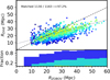 |
Fig. 11 Analogous to Fig. 10, but with ZOBOV and DIVE voids cross-matched for comparison. |
| In the text | |
|
Fig. 12 Slice through the centre of the 2M++ galaxy survey with all voids intersecting it as identified by AVISM when applied to the McAlpine et al. (2025) (non-linear) and Carrick et al. (2015) (linear) density and velocity reconstructions. We use the supergalactic coordinate system (SGX, SGY, and SGZ) defined by De Vaucouleurs et al. (1991). The slice is ≈8 Mpc deep and contains the supergalactic plane (SGZ = 0). The void-finding procedure was restricted to the inner R ≤ 200/h Mpc in both cases. Near cosmological structures are highlighted with capital letters: the Virgo (V), Hydra-Centaurus (H), Norma (N), Shapley (S), and Perseus (P) clusters together with the Sculptor (S), Hercules (H), and Boötes (B) voids (Tully et al. 2019). Voids from the linear catalogue matching that from the non-linear with DSC coefficients larger (smaller) than 0.4 are displayed using the same colour and continuous (dotted) lines. The grey scale displays integrated density contrast. |
| In the text | |
Current usage metrics show cumulative count of Article Views (full-text article views including HTML views, PDF and ePub downloads, according to the available data) and Abstracts Views on Vision4Press platform.
Data correspond to usage on the plateform after 2015. The current usage metrics is available 48-96 hours after online publication and is updated daily on week days.
Initial download of the metrics may take a while.