| Issue |
A&A
Volume 704, December 2025
|
|
|---|---|---|
| Article Number | A9 | |
| Number of page(s) | 21 | |
| Section | Planets, planetary systems, and small bodies | |
| DOI | https://doi.org/10.1051/0004-6361/202554625 | |
| Published online | 28 November 2025 | |
Survival of satellites during the migration of a hot Jupiter
1
Observatoire de Genève, Université de Genève,
Chemin Pegasi 51,
1290
Sauverny,
Switzerland
2
Centre pour la vie dans l’Univers de l’Université de Genève,
Genève,
Switzerland
3
Harvard-Smithsonian Center for Astrophysics,
60 Garden Street,
Cambridge,
MA
02138,
USA
4
Faculty of Psychology, UniDistance Suisse,
Brig,
Switzerland
5
Division of Geological and Planetary Sciences, California Institute of Technology,
Pasadena,
USA
6
Jet Propulsion Laboratory, California Institute of Technology,
Pasadena,
USA
7
Physikalisches Institut, Universität Bern,
Gesellschaftsstr. 6,
3012
Bern,
Switzerland
★ Corresponding author: This email address is being protected from spambots. You need JavaScript enabled to view it.
Received:
18
March
2025
Accepted:
9
October
2025
Abstract
We investigated the origin and stability of extrasolar satellites orbiting close-in gas giants, focusing on whether these satellites can survive planetary migration within a protoplanetary disk. To address this question, we used POSIDONIUS, an N-Body code with an integrated tidal model, which we expanded to account for the migration of a gas giant within a disk. Our simulations include tidal interactions between a 1 M⊙ star and a 1 MJup planet, and between the planet and its satellite, while neglecting tides raised by the star on the satellite. We adopted a standard equilibrium tide model for the satellite, planet, and star, and additionally explored the impact of dynamical tides in the convective regions of both the star and planet on satellite survival. We systematically examined key parameters, including the initial satellite-planet distance, disk lifetime (which serves as a proxy for the planet’s final orbital distance), satellite mass, and satellite tidal dissipation. For simulations incorporating dynamical tides in both the planet and star, we also explored three different initial stellar rotation periods. Our primary finding is that satellite survival is rare if the satellite has nonzero tidal dissipation. Survival is only possible for initial orbital distances of at least 0.6 times the Jupiter-Io separation and for planets orbiting beyond ≈0.1 AU. Satellites that fail to survive are either tidally disrupted, as they experience orbital decay and cross the Roche limit, or dynamically disrupted, where eccentricity excitation drives their periastron within the Roche limit. Satellite survival is more likely for low tidal dissipation and higher satellite mass. Given that satellites around close-in planets appear unlikely to survive planetary migration, our findings suggest that if such satellites do exist (as has been recently suggested), another process should be invoked. In that context, we also briefly discuss the claim of the existence of a putative satellite around WASP-49 A b.
Key words: planets and satellites: formation / protoplanetary disks / planet-disk interactions / planet-star interactions / planets and satellites: individual: WASP-49 A b
© The Authors 2025
 Open Access article, published by EDP Sciences, under the terms of the Creative Commons Attribution License (https://creativecommons.org/licenses/by/4.0), which permits unrestricted use, distribution, and reproduction in any medium, provided the original work is properly cited.
This article is published in open access under the Subscribe to Open model. This email address is being protected from spambots. You need JavaScript enabled to view it. to support open access publication.
1 Introduction
Natural satellites are abundant in the Solar System, and yet identifying their equivalents around exoplanets remains a challenge. Despite the rapid advancement of exoplanet detection techniques, finding evidence for exomoons has proven difficult. In recent years, several methods have been proposed, including direct detection by transit (Sartoretti & Schneider 1999) and indirect approaches that infer their presence through transit-timing variations caused by their gravitational influence on the host planet (Kipping 2009). Another approach involves detecting the possible toroidal atmosphere of the host planet, which is composed of material ejected from the moon (or rings, Johnson & Huggins 2006, this method is analogous to observations of the Jovian and Saturnian systems). A relatively recent claim of detection was made in 2018 by Teachey & Kipping (2018), who discussed that the transit signal obtained with the Hubble Space Telescope was compatible with a Neptune-sized exomoon orbiting a super Jupiter. However, Kreidberg et al. (2019) reanalyzed the data and found that a moonless model led to a better fit, concluding that an artifact of the data reduction was likely responsible for the exomoon transit signal reported by Teachey & Kipping (2018). Not technically an exomoon detection, but a sign of circumplanetary disk was proposed by Benisty et al. (2021), suggesting that satellite formation should occur for exoplanets. A more recent potential candidate was announced by Kipping et al. (2022), who claimed the detection of a 2.6 Earth radius satellite at 16 planetary radii from a host Jupiter-sized planet. However, its existence was questioned by Heller & Hippke (2024). One of the most recent tentative discoveries of an exomoon was proposed by Poon et al. (2024), who measured the obliquity of β Pictoris b and proposed that the origin of its high value might be due to the gravitational interaction with a massive moon (similar to what was proposed for Saturn by Saillenfest et al. 2021). Finally, evidence of a much smaller lunar-sized satellite (assumed to have a radius approximately the same as Io’s, i.e., exo-Io) around the planet WASP-49 A b in transit spectroscopy was suggested by Oza et al. (2019). It remains unclear whether such a satellite could form in situ (similar to hot close-in gas giant planets; e.g., Batygin et al. 2016) at such closein distances given the increased planetary radius during gas giant formation (e.g., Mordasini 2018). Recently, a recent Doppler redshift detection suggests this satellite may currently be on an ~ 8 hour orbit (Oza et al. 2024), based on ongoing high-resolution spectra measurements of its alkali mass flux. The existence of this putative satellite raises many questions about its formation and evolution. A recent confirmation of the Doppler-shifted sodium signature of WASP-49 A b I was made by KECK/HIRES (Unni et al. 2025). Although the neutral sodium signature of the exomoon is suggestive, the orbital period remains unconstrained from 6- to 11-hour circular orbits (Sucerquia & Cuello 2025) encouraging more dynamical scrutiny. A potential satellite on an orbit shorter than 15 hours around the hot Saturn WASP-39 b has also been recently suggested based on variability in the SO2 absorption observed with JWST (Oza et al. 2025).
In this vein, many studies look at the possibility of satellite survival around gaseous planets or sub-Neptunes (e.g., Alvarado-Montes et al. 2017; Quarles et al. 2020; Dobos et al. 2021; Hansen 2023; Makarov & Efroimsky 2023; Patel et al. 2025). The survival of satellites mainly depends on their tidal interaction with the host planet. Satellites are close enough to their host planet to experience tidal forces: the tide raised by the planet on the satellite (satellite tide) and the tide raised by the satellite on the planet (planetary tide). The satellite tide is important for satellites on eccentric orbits, with a nonsyn-chronous rotation and an obliquity. Most of the time, the satellite tide leads to a decrease in the eccentricity, accompanied by an inward migration. The planetary tide is potentially important in a wider range of configurations, and the outcome of the evolution depends on where the satellite is relative to the corotation radius: the orbital distance at which the satellite’s orbital frequency matches the rotation frequency of the planet. If the satellite is beyond this corotation radius, it will migrate outward (as the moon or the satellites of Saturn do; Crida & Charnoz 2012). However, if the satellite is inside the corotation radius, it will migrate inward and eventually fall onto the planet (e.g., Phobos, Mignard 1981).
The timescale of the evolution depends on the characteristics of both planet and satellite, such as their mass, radius, and their internal structure. Depending on their internal structure, particularly whether they have solid and/or liquid layers, the equilibrium tide and/or the dynamical tide can significantly impact the evolution. On the one hand, the equilibrium tide is the result of the hydrostatic adjustment of an extended body perturbed by the presence of another body. One of the most used equilibrium tide models is the constant time lag model (or CTL model; e.g., Mignard 1979; Hut 1981; Eggleton et al. 1998; Leconte et al. 2010; Bolmont et al. 2011, 2015, 2020), which assumes that the bodies are weakly viscous. It is thought to accurately describe the response of gas giants, but is less effective for rocky bodies (in particular, it cannot reproduce the spin-orbit resonances, as observed for Mercury; e.g., Makarov & Efroimsky 2013). On the other hand, the dynamical tide is a wave-like response to the perturbing potential (e.g., Zahn 1975). In particular, in the convective regions of stars or in the gaseous layers of giant planets, inertial waves can propagate (e.g., Ogilvie & Lin 2004, 2007; Guenel et al. 2014). These waves contribute to additional dissipation, which can be several orders of magnitude higher than that of the equilibrium tide (e.g., Mathis 2015). This additional dissipation can lead to a tidal evolution that is different from what we expect based solely on the equilibrium tide (Bolmont & Mathis 2016; Bolmont et al. 2017; Gallet et al. 2017, 2018). Bolmont & Mathis (2016) showed that for a hot Jupiter orbiting a fast-rotating star, the stellar dynamical tide could lead to a significant outward migration of the planet. Similarly, a satellite around a Jupiter-sized planet can excite tidal inertial waves in the fluid layers of the planet (e.g., for Jupiter, Dhouib et al. 2024).
The dissipation in Jupiter is well constrained thanks to accurate and long-term astrometric measurements of the satellites’ orbits (e.g., Lainey 2016)1. In particular, Lainey et al. (2009) measured QJup ≈ 104 for the frequency of Io, a low value (compared to past estimates; see Goldreich & Nicholson 1977 and the next paragraph) likely driven by the dynamical tide in the planet’s fluid envelope (Ogilvie & Lin 2004). Using a similar value of QHJ ≈ 105, some studies have proposed that satellites around hot Jupiters may not survive over gigayear timescales as they gradually spiral into their host planet (e.g., Barnes & O’Brien 2002).
However, depending on whether the dynamical tide is excited or not, estimates of the tidal dissipation can vary by several orders of magnitude. Estimates of the turbulent viscosity of Jupiter led Goldreich & Nicholson (1977) to suggest a tidal dissipation factor for Jupiter to be QJup ≈ 1012 (compatible with a very weak equilibrium tide), which has also been discussed in detail by Ogilvie & Lin (2004); Wu (2005); Ogilvie & Lin (2007). This value is significantly larger than the tidal Q measured for Jupiter or Saturn, implying weak tides and negligible satellite migration. Because a hot Jupiter is expected to be in synchronous rotation with its orbital motion around the star, Cassidy et al. (2009) argued that a satellite cannot excite the dynamical tide in the planet. Using a similarly high value of QHJ, they showed that a hot Jupiter could host a satellite as massive as Earth over gigayear timescales. Notably, Cassidy et al. (2009) included the gravitational influence of the star on the satellite in their study. Another example is Oza et al. (2019), who suggested that a tidal QHJ could be as high as ~ 1010 based on the lack of Na I detections at close-in orbits and on dynamical arguments from Goldreich & Nicholson (1977). Hence, the choice of planetary dissipation is key to studying the survival of the satellites.
We consider here the dynamical evolution of a satellite, previously formed around a hot Jupiter that subsequently migrates inward to less than 0.1 AU from its star (see Fig. 1 for a schematic setup). While one study has examined the fate of moons around hot Jupiters in the high-eccentricity migration scenario (Trani et al. 2020), our focus here is on the fate of moons around around a Jupiter-mass planet undergoing Type II migration. The simulations we present aim to assess the likelihood, based on our assumptions, of satellite survival during the final stages of migration of the planet while accounting for the influence of the dynamical tide in both the star and planet.
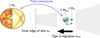 |
Fig. 1 Schema of the simulation setup. An Io-like satellite orbits around a Jupiter-like planet with a solar-like host star. |
2 The model
To describe the evolution of the planet-satellite system, several mechanisms should be considered. First, the gravitational interactions between each body (Section 2.1); second, the interaction between the planet and the disk, which drives the system’s evolution (Section 2.2); and finally, the tidal interactions between the planet and the satellite, as well as between the planet and the star (Section 2.3).
2.1 N-body integration
We used the open-source N-body code POSIDONIUS (Blanco-Cuaresma & Bolmont 2017; Bolmont et al. 2020, Gomes et al. 2021, Revol et al. 2024 Blanco-Cuaresma & Bolmont, in prep.). POSIDONIUS computes the evolution of multi-planet systems while accounting for various additional effects, including tidal interactions (see Section 2.3) and the disk interaction (see Section 2.2).
POSIDONIUS includes several evolutionary tracks for different objects such as solar-like stars (e.g., Gallet et al. 2017) and for Jupiter-mass planets (Leconte & Chabrier 2013). These tracks allow to account for the radius evolution of the star and giant planet as they age. As tidal interactions have a strong dependence on the radii of the bodies, it is therefore important to account for that evolution (see Section 2.3).
POSIDONIUS provides different integration schemes, and here we use IAS15 (Rein & Spiegel 2015), which is an adaptive timestep Gauss-Radau quadrature integrator. Unlike symplec-tic integrators, this integrator does not assume the existence of a dominant massive body (e.g., the host star) at a fixed reference position, such as the origin of the coordinate system. This flexibility allows us to configure the simulation so that tidal interactions between the star and the planet, as well as between the planet and the satellite, are both consistently computed, without requiring modifications to the existing tidal model. However, IAS15 is computationally expensive and significantly slower than a symplectic integrator like WHFast (Rein & Tamayo 2015, which is also included in POSIDONIUS). As a result, the duration of our simulations is limited, with the longest simulations only extending up to 5-6 million years.
2.2 Migration of the hot Jupiter
POSIDONIUS accounts for planetary migration following the planet type II migration prescription of Mordasini (2018) and Alibert et al. (2013). In this work, however, we are not looking to simulate the full migration from a few AU down to a few hundredth of AU. We only focus on the last part of it (from 0.15 AU on), as it is where the gravitational effect of the star starts to be important for the evolution of the satellites. As the order of magnitude for the satellite accretion in a circumplanetary disk is of the order of ~104−105 yr (e.g., Canup & Ward 2002; Ronnet & Johansen 2020; Batygin & Morbidelli 2020), we consider the satellites to be fully formed by the time the planet reaches 0.15 AU. This also allows us not to account for a circumplanetary disk, which is out of the scope of this study.
The acceleration associated with planetary migration in the disk is given as (Fogg & Nelson 2007; Alibert et al. 2013)
 (1)
(1)
where v is the velocity vector of the planet and τmig is the migration timescale, defined as
 (2)
(2)
Here αp is the semimajor axis of the planet and ȧp its time derivative. Similarly, the accelerations associated with eccentricity damping and the inclination damping are given by
 (3)
(3)
and
 (4)
(4)
where r is the position vector of the planet, r is its norm, τe and τi are the eccentricity and inclination damping timescales, and k is the vertical unit vector. Here we assume that both the eccentricity and inclination damping timescales are equal to 0.1 τmig (Alibert et al. 2013).
To compute the migration, eccentricity, and inclination damping accelerations, one needs to estimate the migration timescale τmig, and therefore the time derivative of the semimajor axis, ȧp. For type II migration, we assume that the time derivative of the semimajor axis (i.e., the migration rate, ȧp) is limited by viscous transport within the disk (Alibert et al. 2005; Mordasini 2018) and is therefore given by
 (5)
(5)
where ur is the local radial velocity of the gas, Σg(r, t) is the surface density of the gas, and Mp is the mass of the planet. The radial velocity of the gas is given by ur = −3ν/(2ap), where ν is the viscosity of the disk. We use an α-disk prescription (Shakura & Sunyaev 1973) so that the α viscosity parameter is given by
 (6)
(6)
where H is the vertical scale height, Ω is the Keplerian frequency, and cs is the speed of sound. The α viscosity parameter is usually between 10−3 and 10−2 (Mordasini et al. 2009) and in this study we choose a value of 10−2 (see Table 1). The speed of sound is given by
 (7)
(7)
where kB is the Boltzmann constant, T(r) the temperature of the disk at r, μ the mean molecular weight, and mH the mass of a hydrogen atom. The temperature of an optically thin disk is given by (Ida & Lin 2004)
 (8)
(8)
Finally, we adopt the protoplanetary disk density profile from Lynden-Bell & Pringle (1974) and assume a simple exponential decrease to mimic the disk’s lifetime. The corresponding surface disk density is given by
 (9)
(9)
where r is the radial distance to the star, t is the time, τdisk is the disk lifetime, Σg(t = 0, r) is the initial density profile given by
![Mathematical equation: \Sigma_g(t=0,~r) = \Sigma_0 \left(\frac{r}{1\;{\rm AU}}\right)^{-1}~\exp\left[-\frac{r}{R_{\rm out}}\right]\left(1-\sqrt{\frac{r}{R_{\rm in}}}\right),](/articles/aa/full_html/2025/12/aa54625-25/aa54625-25-eq10.png) (10)
(10)
where Σ0 is a reference disk density, and Rin and Rout are respectively the inner radius and the characteristic outer radius of the disk (the disk does not stop at Rout. The default parameters are listed in Table 1.
The evolution of the density profile over time is illustrated in Figure 2 for a disk of τdisk = 0.1 Myr, Rin = 0.01 AU and Rout = 100 AU, and Σ0 = 1000 g/cm2. Initially, the profile exhibits a maximum close to the inner edge, followed by a gradual decrease toward the outer parts of the disk. For radii higher than Rout, the decrease becomes significantly steeper. The density, and consequently the mass, of the disk decrease with time according to Eq. (9). In the framework that we are using for mimicking a type II migration (Alibert et al. 2005; Mordasini 2018), we note that there is no gap in the surface density profile.
To analyze the impact of type II migration on a Jupiter-mass planet, we run a POSIDONIUS simulation where the planet begins its evolution at 0.15 AU around a 1 Myr old star (Figure 3). The simulation accounts for four key processes: (1) disk interactions, (2) tidal interactions, (3) stellar evolution, and (4) planetary evolution. The top panel of Figure 3 (dashed-lines) illustrates how the migration process depends on the disk lifetime τdisk. The results corresponding to the dashed lines were calculated for weak tides (equilibrium tides, see next Section 2.3), which is very similar to what we obtain with no tides at all.
A shorter disk lifetime results in migration halting at a greater distance from the star. For a duration of τdisk = 5000 yr, the planet stops at ≈0.13 AU, whereas for the longest duration considered of τdisk = 50 000 yr, the planet comes as close as ≈0.03 AU. The disk lifetime can therefore be used as a proxy for final planet position.
Disk parameters.
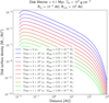 |
Fig. 2 Evolution of the disk surface density Σg(r, t). |
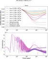 |
Fig. 3 Evolution of the semimajor axis and eccentricity of a Jupiter-mass planet due to type II migration for different disk lifetimes τdisk and different assumptions on the stellar tide. The dashed lines correspond to the case where only the equilibrium tide in the star is accounted for; the solid lines correspond to cases where both the equilibrium tide and dynamical tide are taken into account (initial fast stellar rotation period of 1 day). We note that the rotation of the star is evolving, here mainly due to the contraction of the radius, and its evolution is encoded in the corotation radius curve (i.e., where the orbital frequency is equal to the stellar spin). For clarity, we only plot two cases in the bottom panel (τdisk = 2 × 10⁴ yr and 5 × 10⁴ yr). The equilibrium tide is still represented with dashed lines, but also with transparency to ease identification. |
2.3 Tidal model
To model tidal interactions, POSIDONIUS follows the equilibrium tide prescription of Bolmont et al. (2015), implementing the constant time lag model (Mignard 1979; Hut 1981; Eggleton et al. 1998). The governing equations are detailed in Bolmont et al. (2020), where POSIDONIUS was applied to the TRAPPIST-1 system (Gillon et al. 2017). Although it features an implementation of the constant time lag model, we adopt different assumptions for the three types of bodies in this study (a satellite, a planet and a star). In the following, regardless of how the tidal dissipation is expressed (whether as a quality factor Q, a time lag Δt, or a tidal dissipation factor σ), the satellite, planet, and star will be denoted by the subscripts sat, p, and ★, respectively. The specific assumptions and models are outlined below.
Satellite parameters.
2.3.1 Equilibrium tide in the satellite
For the satellite, we use a simple constant time lag model, where the dissipation is governed by the quantity k2,satΔtsat, where k2,sat is the satellite’s Love number of degree two, and Δtsat is its time lag (assumed to be independent of the excitation frequency in this model). As a reference, we use as Earth’s time lag value of Δt⊕ = 638 s (Neron de Surgy & Laskar 1997). POSIDONIUS expresses dissipation through the factor σ, as introduced in Eggleton et al. (1998)
 (11)
(11)
where Rsat is the satellite’s radius. The corresponding values used in this study are listed in Table 2 for the two satellites masses considered: 1 MIo and 10 MIo. For the 10 MIo satellite, the radius is computed assuming a density equal to that of Io’s.
2.3.2 Equilibrium tide and dynamical tide in the star
To model tidal interactions in the star, we adopt the formalism of Bolmont & Mathis (2016), which is based on the work of Ogilvie (2013) and Mathis (2015). This approach allows us to retain the constant time lag model while incorporating the contribution of the dynamical tide in the specific case of circular and coplanar orbits. In this context, the dynamical tide refers to the tidal inertial waves that can be excited in the star’s convective region. These waves are driven by the Coriolis acceleration, while the dissipation results from turbulent friction exerted by convective eddies on the waves. These waves are excited for a very specific range of excitation frequencies ω, which depends on the star’s rotation frequency as is defined by ω ∈ [−2Ω*,2Ω*]. Within this range, the dynamical tide introduces additional dissipation beyond the classical equilibrium tide. Outside of [−2Ω*, 2Ω*], only the equilibrium tide contributes to the system’s tidal evolution. For the equilibrium tide, we assume a dissipation of σ* = 4.992 × 10−66 g−1 cm−2 s−1 following Hansen (2010) and Bolmont et al. (2015).
Ogilvie (2013) showed that the frequency-averaged dissipation of these tidal waves depends on the structural parameters of the star (radius, mass and radius aspect ratio) and its rotation. As the star evolves (shrinking or expanding, developing a radiative core, and experiencing changes in rotation), its tidal dissipation also evolves (Mathis 2015). In particular, Bolmont & Mathis (2016) found that this additional dissipation, being significantly stronger than the usual equilibrium tide dissipation, leads to a drastically different early evolution of massive planets when the dynamical tide is accounted for.
This formalism was incorporated in POSIDONIUS using the expression for the time lag Δτ*, as given in Bolmont & Mathis (2016). The following expression is valid for a circular coplanar orbit, for which the excitation frequency is ω = 2(n – Ω*)
 (12)
(12)
where k2,* the Love number of the star, and Q′s,* represents the frequency-averaged of the structural dissipation due to the tidal inertial waves excited in the star’s convective envelope. Here, we compute the frequency-averaged structural dissipation factor Q′s,* from stellar evolution models (Gallet et al. 2017), using the following formula:
![Mathematical equation: \lefteqn{\left<{\mathcal D_\star}\right>_{\omega}=\int^{+\infty}_{-\infty} \! {\rm Im} \left[k_2^2(\omega)\right] \,\frac{\mathrm{d}\omega}{\omega} = \hat{\epsilon}_\star^{2} \frac{3}{2Q'_{s,\star}} }\\](/articles/aa/full_html/2025/12/aa54625-25/aa54625-25-eq13.png) (13)
(13)
![Mathematical equation: \begin{aligned} && = \hat{\epsilon}_\star^2 \left(\frac{\Rs}{\Rsun}\right)^3\left(\frac{\Msun}{\Ms}\right) \frac{100 \pi}{63} \left(\frac{\alpha_\star^5}{1-\alpha_\star^5}\right)\left(1-\gamma_\star\right)^2 \left(1-\alpha_\star\right)^4\\ &&\times\left(1+2\alpha_\star+3\alpha_\star^2+\frac{3}{2}\alpha_\star^3\right)^2\left[1+\left(\frac{1-\gamma_\star}{\gamma_\star}\right)\alpha_\star^3\right]\nonumber\\ &&\times\left[1+\frac{3}{2}\gamma_\star+\frac{5}{2\gamma_\star}\left(1+\frac{1}{2}\gamma_\star-\frac{3}{2}\gamma_\star^2\right)\alpha_\star^3-\frac{9}{4}\left(1-\gamma_\star\right)\alpha_\star^5\right]^{-2}\nonumber \end{aligned}](/articles/aa/full_html/2025/12/aa54625-25/aa54625-25-eq14.png) (14)
(14)
with
 (15)
(15)
The dependence of the dissipation on the stellar rotation is encapsulated in the ε̂ parameter, defined as
 (16)
(16)
where Ω⊙,c is the critical angular velocity of the Sun. As with the satellite dissipation factor in Eq. (11), the stellar dissipation factor σ* is derived from Δτ*, the Love number of the star k2,*, and the radius of the star R*.
To validate our implementation of the dynamical tide, we reproduced the results of Bolmont et al. (2017) for a Jupiter-mass planet orbiting a Sun-like star with solar metallicity, considering three different initial stellar rotation periods: 1, 3 and 8 days (see Appendix A). Figure 3 illustrates the evolution of the semimajor axis and eccentricity of a Jupiter-mass planet, accounting for both the migration in the disk and tidal evolution. Different line styles represent different assumptions: dashed lines correspond to a scenario where only the equilibrium tide is taken into account, while solid lines depict a case where both equilibrium and dynamical tides are included. When the additional dissipation of the dynamical tide is considered, the planets do not migrate as close to the star because the stellar tide efficiently pushes them outward, counteracting the disk-driven migration. As a result, a migrating Jupiter-mass planet orbiting an initially fast-rotating Sun-like star is unlikely to be found very close to its host star within the first few million years of its lifetime. The bottom panel of Fig. 3 also tracks the planet’s eccentricity, which is initially set to zero. In a numerical integration such as those performed by POSIDONIUS, a small residual eccentricity can persist due to numerical artifacts (see Bolmont et al. 2015), as seen in Fig. 3. During the first 10000 yr of evolution, this eccentricity is damped by the disk. As the disk dissipates, a slight excitation of the eccentricity occurs. When the dynamical tide is included (solid lines), the stellar tide subsequently damps the eccentricity, an effect that is more pronounced for the planets closer to the star. Conversely, if only the equilibrium tide is considered (dashed line), the eccentricity is not as strongly damped; however, its value remains well under 10−6.
In our application to a star-planet-satellite system, the orbits are not perfectly circular. The eccentricity of the planet remains small (see Figs. 3 and 4), which means the evolution of the planet due to the stellar tide should be as correct as our formalism allows. However, the eccentricity of the satellite can be high. In that case, other excitation frequencies are excited in addition to the main semi-diurnal frequency ω = 2(n − Ω*), which would enhance dissipation within the planet. Taking into account these additional modes might lead to shorter migration and eccentricity damping timescales for the satellite. As a result, we are using a prescription that technically falls outside its formal applicability limits. However, implementing a more accurate formalism for the star would introduce significant complexity. A proper treatment would require abandoning the convenient, simple, and computationally efficient constant time lag model in favor of accounting for the frequency dependence of tidal dissipation in stars and planets by implementing the Kaula formalism (Kaula 1964). These improvements have already been implemented in POSIDONIUS for the planets by Revol et al. (2024), and are currently being implemented for stars (Kwok et al. in prep.). Given the planet eccentricity remains small and the dynamical tide has a non-negligible effect on close-in planets (Bolmont & Mathis 2016), we opted to use this formalism despite its limitations. While not perfect, this approach constitutes an improvement over the original constant time lag model, as it allows the time lag to evolve with the stellar and planetary parameters.
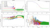 |
Fig. 4 Evolution of a 1 MIo satellite orbiting a migrating Jupiter-mass planet for different initial distances of the satellite. Here the disk lifetime is 3 × 10⁴ yr, the initial rotation period of the star is 1 day and the dissipation in the satellite is taken to be 0. The top left panel shows the evolution of the semimajor axis of the satellite (solid colored lines); the shaded colored lines represent the periastron and apoastron. The gray dotted line represents the radius of the planet, the black dash-dotted line represents the Roche radius, the black dashed line the corotation radius (where the satellite’s mean motion is equal to the spin of the planet), and the gray dashed line represents one-half of the Hill radius of the planet. The bottom left panel shows the evolution of the satellite’s eccentricity. The top right panel shows the evolution of the semimajor axis of the planet (solid colored lines). The black dashed line represents the corotation radius (where the planet’s mean motion is equal to the spin of the star). The bottom left panel shows the evolution of the planet’s eccentricity. |
2.3.3 Equilibrium tide and dynamical tide in the planet
For the planet, we adopt a similar approach as the for the star. The gas giant, with mass Mp, radius Rp, and density ρp, is modeled as a two-layer structure consisting of a homogeneous and a fluid envelope. The core, with radius Rc, mass Mc, and density ρc, is surrounded by a fluid envelope where the dissipation of inertial waves occurs.
For the equilibrium tide, we assume a dissipation value of σp = 2.006 × 10−60 g−1 cm−2 s−1, corresponding to the dissipation of a purely convective body (Hansen 2012; Bolmont et al. 2015)2.
For the dynamical tide, we compute the frequency-averaged structural dissipation factor Q'sp using data from Leconte & Chabrier (2013) and applying the formalism of Ogilvie (2013) (see also Guenel et al. 2014). The frequency-averaged dissipation due to tidal inertial waves in the fluid envelope of a piecewise-homogeneous fluid body with a solid core of a different density is given by Ogilvie (2013); Guenel et al. (2014)
![Mathematical equation: \left<{\mathcal D_{p}}\right>_{\omega} &=\int^{+\infty}_{-\infty} \! {\rm Im} \left[k_2^2(\omega)\right] \,\frac{\mathrm{d}\omega}{\omega} = \hat{\epsilon}_p^{2} \frac{3}{2Q'_{s,p}} \\](/articles/aa/full_html/2025/12/aa54625-25/aa54625-25-eq17.png) (17)
(17)
 (18)
(18)
![Mathematical equation: &\quad\times\left[1+\frac{1-\rho_p/\rho_c}{\rho_p/\rho_c}\alpha_p^3\right]\left[1+\frac{5}{2}\frac{1-\rho_p/\rho_c}{\rho_p/\rho_c}\alpha_p^3\right]^{-2},](/articles/aa/full_html/2025/12/aa54625-25/aa54625-25-eq19.png) (19)
(19)
where αp is the planet’s radius aspect ratio, defined as αp = Rc/Rp, and εp is set with respect to the Sun as for the stellar tide3:
 (20)
(20)
We note that Equation (17) differs from Equation (13), where the core was assumed to be fluid rather than rocky.
Following Guenel et al. (2014), we assumed a core mass of 6.35 M⊕ and of radius 1.38 R⊕ to calculate Q′sp. Core mass and radius are taken to be constant while the radius of the planet Rp evolves as the planet ages (following Leconte & Chabrier 2013).
3 Numerical setup and initial conditions
In this study, we consider a Jupiter-mass planet orbiting a Sun-like star while hosting a satellite. The initial age of the Jupiter-mass planet and the star is set to 1 Myr. The initial rotation periods of the planet and the satellite are 13 and 10 hours, respectively, with both bodies having an initial obliquity of 0.2 rad.
The parameters varied in our simulations include:
the initial semimajor axis of the satellite (0.3, 0.4, 0.6, 0.8, 1.0 aIo),
the mass of the satellite (1 MIo, 10 MIo),
the dissipation in the satellite ([0, 10−4, 10−2, 10−1, 1.0] × Δ t⊕),
the disk lifetime (5000,7000,10 000,12 500,20 000, 35 000, 50 000 yr),
the initial stellar rotation period (1 day, 3 days, 8 days).
Since our primary focus is on the final stages of the planet migration, we initialize the simulations with a planet at 0.15 AU from the star. At that initial star-planet distance, the outer satellite (1.0 aIo) is initially well within the 0.5 RHill stability criterium (Domingos et al. 2006) and we note a limited eccentricity excitation (≲ 10−2). This also justifies the relatively short disk lifetime compared to the typical migration timescales required to explain the inward migration of a Jupiter-like planet from 5 AU to a few 10−2 AU. The integration timescale is of 5-6 Myr, for the simulations with surviving satellites. For the others, the integration is stopped when the satellites collides with the planet. Due to long computation time for the closest satellite-planet distances, limited resources and overall footprint of these calculations, we note that some simulations were not continued to reach 5 Myr.
4 Between a rock and hard place
The survival of the satellite is constrained by two key processes: tidal inward migration and eccentricity excitation, both of which can ultimately lead to a collision. The relative significance of these processes depends on two main factors: (1) the disk lifetime and density, which serve as proxies for the final star-planet distance resulting from the migration, and (2) the dissipation properties of the various bodies involved. We discuss these influences in the following sections. However, before getting into a broader analysis, we first illustrate the possible outcomes through a specific case in which only the equilibrium tide in the star and planet is considered.
4.1 Equilibrium tide in star and planet
Since most tidal studies consider only the equilibrium tide, we begin our analysis with this familiar setup. In this section, we first discuss the influence of the satellite’s initial semimajor axis (Section 4.1.1), followed by the effects of disk lifetime (Section 4.1.2), satellite dissipation, and satellite mass.
4.1.1 Initial distance of the satellite
The evolution of a 1 MIo satellite orbiting a migrating Jupiter-mass planet varies depending on its initial orbital distances, as illustrated in Figure 4. In this case, we assume a disk lifetime of 3 × 10⁴ yr. Under these conditions, the planet reaches a final distance of 0.057 AU after slightly more than 100 000 years of migration (top right panel of Fig. 4). We can therefore consider here the disk to be fully dissipated at around 100 000 years after the beginning of our simulation. Throughout the migration, the planet’s eccentricity remains low, primarily due to the damping effect of the disk (bottom right panel of Fig. 4). As the planet approaches the star in the final stage of the migration, its rotation evolves in response to the shifting corotation radius, as shown in the top left panel (black dashed lines). Due to the tide raised by the star in the planet, the planet’s rotation gradually slows down toward the pseudo-synchronous rotation, which, for such low eccentricities, closely approximates synchronous rotation (see bottom right panel). In this specific case, the final pseudo-synchronous period is approximately 5 days and the corresponding plot can be seen in Appendix C.1.
In the scenario depicted in Fig. 4, we assume no dissipation in the satellite. The satellite’s fate varies depending on its initial orbital distance4. First, consider a satellite that begins its orbit beyond 0.8 aIo (the two outermost satellites). As the planet migrates inward, the increasing gravitational influence of the star excites the satellite’s eccentricity. This effect is illustrated by the gray dot-dashed line, which represents one-half of the Hill radius, RHill, of the planet. This follows the stability limit proposed by Domingos et al. (2006), who suggested that satellites remain stable within approximately ~0.5 RHill. The Hill radius marks the distance at which the satellite experiences equal gravitational attraction from both the star and the planet. As the planet moves closer to the star, the Hill radius shrinks, intensifying the eccentricity excitation. For the two outermost satellites, this excitation is strong enough to bring their periastron distance within the Roche radius of the planet. As a result, the satellite undergoes tidal disruption, effectively leading to a collision with the planet. We refer to this outcome as dynamical disruption, distinguishing it from the alternative fate described next, which occurs under different migration conditions.
Next, we consider the fate of the innermost satellite. The satellite initially located at 0.3 aIo undergoes inward migration due to the tide raised by the satellite in the planet, as we have assumed no dissipation in the satellite itself. This migration has two contributing factors: 1) since the satellite orbits below the corotation radius (represented as a black dashed line), the planetary tide acts to decrease the semimajor axis; 2) the satellite’s nonzero eccentricity induces eccentricity-driven tidal migration. Following an initial stage of eccentricity excitation due to the approaching star, the eccentricity is then damped and the semimajor axis also decreases (blue, orange and green curves). It is important to note that, in this case, eccentricity damping is driven solely by tides raised inside the planet, which is significantly less efficient than the dissipation that would occur if tides were raised in the satellite (a process explored later in this study). Due to the satellite’s relatively low mass, the migration induced by the tide raised in the satellite (contributing factor 2 above) dominates its evolution. Moreover, this effect is further amplified by an additional mechanism: as the star approaches, it triggers eccentricity excitation, preventing the eccentricity from fully damping to zero. This eccentricity leads to a slightly faster migration compared to a scenario with zero-eccentricity. For the innermost satellite, this tidally-induced inward migration progresses rapidly enough that it reaches the Roche radius of the planet in about 100 000 yr, resulting in tidal disruption. We refer to this outcome as tidal disruption, distinguishing it from the previously described dynamical disruption, as the underlying mechanism differs.
The satellite initially located at 0.4 aIo follows a very similar evolutionary path, though it does not collide within the simulation time. Due to its greater initial distance from the planet, its inward migration progresses more slowly, while its eccentricity excitation is slightly more pronounced. Although the satellite remains intact within the simulation period, it is likely to reach the Roche radius in a few million years. The exact timescale for this eventual disruption depends on the dissipation assumed for the planet.
The satellite initially located at 0.6 aIo follows an intermediate evolutionary path. It undergoes significant eccentricity excitation due to the approaching star, and this enhanced eccentricity leads to some tidal evolution. In particular, the planetary tide dampens the eccentricity, leading to a very slow decrease in the semimajor axis; we note that during this phase, due to angular momentum conservation, the pericenter distance does not decrease. Initially, the satellite orbits beyond the corotation radius, where the planetary tide acts to increase its semimajor axis. However, because the satellite is not massive enough, this outward effect remains negligible. At approximately 1.5 Myr, the satellite crosses the corotation radius, after which both migration mechanisms (one driven by the planet’s nonsynchronous rotation and the other by the satellite’s nonzero eccentricity) begin working in the same direction: inward migration. However, this process is quite long. The eccentricity previously excited by the approaching star will be damped until it reaches an equilibrium between tidal damping and eccentricity excitation (e.g., Batygin et al. 2009; Bolmont et al. 2013). Once this equilibrium is reached, the satellite will experience a satellite-tide induced inward migration similar to the satellite at 0.3 and 0.4 aIo (in blue and orange), enhanced by the slow inward migration due to the weak planetary tide. From this point forward, the satellite’s fate is sealed, and it will inevitably reach the Roche radius. Determining the exact moment of its disruption would require a longer integrating time, becoming very computationally expensive.
In summary, in this particular example, no satellite is expected to survive the evolution. They are either dynamically disrupted early on due to the eccentricity excitation caused by the approaching star, or they are (or will be) tidally disrupted following a tidally-induced inward migration.
4.1.2 Disk lifetime - or planet final distance
The disk lifetime plays a crucial role in determining the survival of the satellites. A longer disk lifetime allows the planet to migrate closer to the star, increasing eccentricity excitation and thereby raising the likelihood of the satellite colliding with the planet.
To illustrate the effect of disk lifetime, we compare the evolution of the satellite for the two extreme values of the disk lifetime considered: 5 × 10³ years in (left column of Figure 5) and 5 × 10⁴ years (right column of Figure 5). As previously discussed, the disk lifetime τdisk serves as a proxy for the planet’s final position relative to the star. In the previous section, with τdisk = 3 × 10⁴ yr, the planet completed its migration at approximately 0.057 AU. For a shorter disk lifetime of τdisk = 5 × 10³ yr, the planet settles farther from the star at 0.125 AU. Conversely, with a longer disk lifetime of τdisk = 5 × 10⁴ yr, the planet migrates inward to 0.035 AU.
In the case of the shortest disk lifetime, where the planet settles at 0.125 AU, most satellites appear to survive the evolution. Only the two innermost satellites have either undergone tidal disruption or seem to be evolving toward it. The fate of the satellite initially located at 0.4 aIo remains uncertain. The slight decrease in the corotation radius suggests that this satellite could eventually cross it, following a process similar to that described in Bolmont et al. (2011). If this occurs, the eccentricity-driven inward migration could be counteracted by the outward migration caused by the nonsynchronicity between planet’s rotation rate and the satellite’s orbital frequency. The gradual decrease in corotation is a result of planetary spin-up induced by the planet’s contraction. Because the planet remains relatively distant from the star, this spin-up occurs on shorter timescale than the tidally-induced spin-down, which will eventually slow the planet’s rotation to approximately 15 days (corresponding to a corotation radius increase to about 4 aIo). Although longer simulations would be required to determine the satellite’s precise evolution, it is thus expected to eventually cross the increasing corotation radius, undergo inward migration, and ultimately reach the Roche limit. However, for simulations of satellites that are very close to the planet, the timestep is very small, which means that the simulations are very long. The full computation of the evolution of this satellite would require an unreasonable amount of resources.
In the case of the longest disk lifetime, where the planet settles at 0.035 AU, all the satellites are ultimately lost. The four outermost satellites undergo dynamical disruption due to the eccentricity excitation induced by the approaching star, while the innermost satellite is tidally disrupted. The planet barely has time to reach its final semimajor axis before all the satellites are removed. An interesting consequence of the planet’s proximity to the star is the rapid evolution of its rotation toward the pseudo-synchronous rotation. This effect is evident in the significant increase in the corotation radius over the course of the first few 105 yr of the simulation.
In this scenario, the tidal evolution of the satellites is solely dictated by the tide they raise in the planet, as we assumed no dissipation in the satellite. This represents the most favorable case for the configuration considered here, where only equilibrium tides in the planet and star are taken into account. Including tidal dissipation in the satellite would further increase the probability of tidal disruption. A synthetic visualization of these results are presented in the top left panel of Figure 7 (1.0 MIo and Δtsat = 0.0 Δt⊕), where the different populations are depicted. Satellites that undergo tidal disruption are shown in red (those initially located at asat = 0.3 aIo), while those experiencing tidal decay, likely leading to eventual tidal disruption, are marked in orange. Dynamical disrupted satellites, which are the farthest from the planet in cases with the longest disk lifetime, appear in blue. Surviving satellites are displayed in green. For these surviving satellites, their evolution follows one of two paths: either they undergo a slight outward migration driven by the planetary tide (as long as they stay beyond the corotation radius), or they exhibit no significant migration. The threshold distinguishing non-negligible migration from negligible migration is taken to be 10−4 AU/Myr, corresponding to approximately 0.035 aIo/Myr.
The disk lifetime, or equivalently the planet’s proximity to its star, is a crucial factor in determining satellite survival. As shown in Fig. 7, no satellite remains intact if the planet migrates closer than 0.057 AU. At shorter distances, the outer satellites undergo dynamical disruption, while the inner satellites are likely to experience tidal disruption. Conversely, if the planet remains beyond 0.057 AU, the outer satellites can survive.
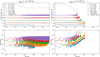 |
Fig. 5 Same as the right column of Figure 4, but for a disk lifetime of 5 × 10³ yr (left column) and 5 × 10⁴ yr (right column). The top row shows the evolution of the orbital distance of the satellites and the bottom row shows the evolution of their eccentricities. For the left column, the final semimajor axis of the planet is 0.125 AU and for the right column, it is 0.035 AU. This difference can be visualized thanks to the gray dashed lines corresponding to one-half of the Hill radius of the planet, which comes much closer to the planet when the τdisk = 5 × 10⁴ yr. |
4.1.3 Increasing the dissipation in the satellite
As previously discussed, assuming zero dissipation in the satellite represents an idealized scenario for satellite survival. In reality, no bodies exhibit zero dissipation, hence we now investigate the impact of varying this parameter. To explore a broad range of possibilities, we vary the dissipation from 0 to 1 time the dissipation of the Earth5. Figure 6 presents the evolution of a 1 MIo satellite for a disk lifetime of 35 000 yr, considering different values of the satellite dissipation and two distinct initial orbital distances: 0.4 aIo (left column) and 0.6 aIo (right column).
The expected effect of increasing dissipation is clearly observed in the top panel of Fig. 6: inward migration occurs on shorter timescales. As dissipation in the satellite becomes increasingly more effective at damping the excited eccentricity (slightly visible with the periastron and apoastron distances: the line is thinner for higher dissipations), migration accelerates, ultimately leading to early tidal disruption.
The bottom panel of Fig. 6 presents another example, offering additional insights. Notably, for the two highest dissipation values (0.1 and 1.0 Δt⊕), the satellite is no longer dynamically disrupted. As the star approaches the planet-satellite system, eccentricity excitation increases, but the effectiveness of tidal damping depends on the level of dissipation. Lower dissipation results in weaker tidal damping, allowing eccentricity to rise unchecked. For the lowest dissipation cases, the periastron distance eventually decreases to the Roche radius, leading to dynamical disruption. Conversely, at the two highest dissipation levels, the satellite tide acts to sufficiently damp the eccentricity to prevent that fate. For 0.1 Δt⊕ (in red), eccentricity damping from 0.3 to 0.1 (bottom right panel) accelerates inward migration, which then slows as the eccentricity drops below 0.1. For 1.0 Δt⊕ (in purple), stronger dissipation limits eccentricity excitation to values below 0.1 (bottom right panel), resulting in a smoother inward migration to 0.1 Δt⊕. Once the eccentricity falls below 0.1, both satellites continue to experience a gradual decrease in semimajor axis and eccentricity until tidal disruption occurs before 106 yr. In that example, the fate of the satellite remains the same: it does not survive, but the dissipation in the satellite changed the nature of its fate from a dynamical disruption to a tidal disruption. The highest the dissipation, the more satellites experience tidal disruption.
A synthetic view of the satellites’ fates across different dissipation values is presented in Figure 7, with dissipation increasing from left to right. The results indicate that higher dissipation leads to a greater minimum star-planet distance required for satellite survival. As dissipation increases from 0 to 0.1 Δt⊕, this survival threshold shifts from 0.077 to 0.125 AU. For 1 Δt⊕, satellite survival becomes impossible at star-planet distances below 0.125 AU, which is the biggest distance considered in this study. Thus, to detect a satellite around a planet orbiting closer than 0.1 AU, the satellite’s internal dissipation must be relatively low.
Given that the heat dissipation on Io is estimated to be approximately 3 W/m2 (e.g., Spencer et al. 2000), we can derive a corresponding ΔtIo to compare with the dissipation values we used in this study (expressed in Δt⊕). Using the formula to compute tidal heating in the framework of the CTL model (Leconte et al. 2010; Bolmont et al. 2013) and extracting the time lag corresponding to Io’s tidal heating yields a value of ΔtIo = 2.7 × Δt⊕ (consistent with actual values of ΔtIo, see Aygün & Cadek 2024). This value exceeds the maximum Δtsat considered in this study. If Io is representative of such exomoons, this suggests that they are unlikely to exist around planets orbiting closer than 0.125 AU to their star. At these small separations, eccentricity excitation caused by the star drives the satellite toward tidal disruption and eventual engulfment.
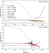 |
Fig. 6 Evolution of the semimajor axis and eccentricity (through apoastron and periastron distances) of a 1.0 MIo satellite for different satellite dissipations. Here the disk lifetime is 35 000 yr, and the disk density 1000 g cm−2. The evolution is shown for two different initial satellite semimajor axes: 0.4 aIo (top panel) and 0.6 aIo (bottom panel). |
4.1.4 Increasing the mass of the satellite
We now examine the evolution of a more massive satellite with a mass of 10 MIo. A higher satellite mass leads to a faster orbital evolution: it induces stronger tidal interactions with the planet, making its migration more sensitive to its position relative to the corotation radius. Additionally, due to its larger radius compared to the 1 MIo satellite, it undergoes a more rapid evolution driven by satellite-induced tides. A synthesized comparison of these effects is presented in Figure 7, allowing for a direct evaluation of differences between the 10 MIo and 1 MIo satellites.
For all the disk lifetimes considered in this study, and as expected, satellites initially located inside the corotation radius undergo tidal disruption more rapidly than their 1.0 MIo counterparts. This trend is evident in Figure 7, all 10 MIo satellites that began at 0.4 aIo experience tidal disruption before 5 Myr (red crosses), whereas their 1 MIo counterparts remain intact (orange crosses).
The fate of satellites initially located outside the corotation radius depends on the disk lifetime under consideration. First, we examine the shortest disk lifetime (5000 yr), which corresponds to a final star-planet distance of 0.125 AU. For satellites with no dissipation, those initially beyond the corotation experience a significantly more pronounced outward migration than their 1.0 MIo counterparts. This effect is evident when comparing the green ticks between top and bottom row of Figure 7 : in the bottom row (10 MIo), the ticks appear brighter, indicating that satellites more frequently migrate outward at a rate exceeding 10−4 AU/Myr, equivalent to 3.6 × 10⁻² aIo/Myr. As dissipation increases, the extent of the outward migration is progressively reduced. For a high dissipation (>0.01 Δt⊕), migration is even reversed for the two outer satellites (0.8 and 1.0 aIo), whose eccentricities are the most strongly excited by the approaching star, driving them into inward migration instead.
Increasing the disk lifetime (or equivalently, decreasing the final star-planet distance) significantly impacts the survival of 10 MIo satellites, just as it does for 1.0 MIo satellites. For the longest disk lifetime considered, no satellite survives. However, the mechanisms leading to their destruction differs from those observed for 1.0 MIo satellites. In particular, due to their greater mass, 10.0 MIo satellites are less susceptible to dynamical disruption and instead undergo tidal disruption. The difference is evident in Figure 7, where the extent of the blue areas, representing dynamically disrupted satellites, is noticeably smaller for 10 MIo (bottom row) compared to 1 MIo (top row).
As observed for 1.0 MIo satellites, survival rates are higher at lower dissipation levels. However, even a small amount of dissipation is sufficient to limit their long-term survival. Satellites initially located outside the corotation radius undergo a more pronounced outward migration, which temporarily spares them from imminent tidal disruption. However, as they migrate outward, they become increasingly influenced by the gravitational pull of the star. This effect enhances their eccentricity, which could ultimately drive their orbit into a slow inward decay, culminating in tidal disruption.
Further details on the influence of the mass of the satellite will be provided in the next section, where we extend our analysis beyond the equilibrium tide and also account for the dynamical tide in both the star and the planet.
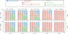 |
Fig. 7 Survival chart of a 1.0 MIo (first row) and a 10.0 MIo (second row) satellite for different satellite dissipations and for equilibrium tides only, from no dissipation (left) to Δtsat = 1 Δt⊕ (right). The fate of the satellites is a function of the disk lifetime (left vertical axis) and the corresponding final semimajor axis of the planet (right vertical axis) and its initial position (horizontal axis). The blue crosses and region correspond to the dynamical disruption scenario. The red crosses correspond to satellites that underwent a tidal disruption within the simulation time (5 Myr), the orange crosses correspond to satellites that are migrating inward at a rate faster than 10−4 AU/Myr. This population (red and orange crosses) is outlined by the red region. The dark green check signs correspond to satellites whose fate is not clear (migration lower than 10−4 AU/Myr). The light green check signs correspond to an outward migration at a rate faster than 10−4 AU/Myr. The green region therefore corresponds to satellites that should survive. The black dashed line shows the final planet semimajor axis below which there is no survival of satellites. |
4.2 Dynamical tide in star and planet
In this section, we incorporate the effects of both the dynamical tide in the star and in the planet, in addition to the equilibrium tide6. When considering only the equilibrium tide in the star, the initial stellar spin has minimal influence. However, incorporating the dynamical tide increases dissipation, thereby accelerating the system’s tidal evolution, which then becomes highly sensitive on the star’s initial rotation rate (see discussions in Bolmont & Mathis 2016). Thus, in addition to assuming only an initial rotation of 1 d (representing a fast rotator), we also consider 3 d (an intermediate rotator) and 8 d (a slow rotator). A summary of outcomes for 1.0 MIo satellites is presented in Figure 8, illustrating results for different satellite dissipation values (different rows) and the three stellar rotation periods considered (different columns). To enable direct comparisons with the equilibrium tide case, the first column of Fig. 8 reproduces the corresponding results from Fig. 7. A similar summary for 10 MIo satellites is provided in Figure D.1 of Appendix D with the corresponding discussion.
When accounting for the dynamical tide, the orbital evolution of the planet differs significantly, as shown in Fig. 3 for a fast-rotating star. Depending on the star’s initial rotation period, the planet may be efficiently pushed outward (for P* = 1 day) or collide in the star (P* = 8 day for the two longest disk lifetimes). In the latter case, satellite survival is impossible. Furthermore, incorporating the dynamical tide in the planet enhances dissipation, making planetary-tide driven migration significantly more efficient. As a result, satellites inside the corotation are engulfed more rapidly than when considering only the equilibrium tide, while those outside corotation migrate outward at a faster rate than before.
This observation helps explain one of the major differences between the equilibrium tide and the dynamical tide cases in Fig. 8. By comparing the maps for the same disk dissipation timescale τdisk, we observe that satellites tend to survive more frequently when the dynamical tide is included. This effect is particularly pronounced at the highest satellite dissipation values considered. For Δtsat = 1.0 Δt⊕, no satellite survived in the equilibrium tide case (Fig. 8, first column). However, in the dynamical tide case, the satellite initially located at 0.6 aIo survives at the largest final star-planet distances (second to fourth columns). It is important to note that the maximum star-planet distance for the dynamical tide case exceeds that in the equilibrium tide case for the same disk lifetime. Thus, disk lifetime alone is no longer a reliable proxy for planetary distance; instead, we must directly pay attention to the planet’s final orbital distance. As shown in Figure 8, one key reason why satellites survive even at the longest disk lifetime considered (50 000 yr) around an initially fast-rotating star (second column), for satellite dissipation values ≤0.1 Δt⊕, is the planet’s final semimajor axis is significantly larger (0.1077 AU) than in the equilibrium tide case (0.035 AU, see first column).
This behavior is illustrated in Figure 9 for a disk lifetime of 35 000 yr, though the same trend holds for 50 000 yr. The planet’s orbital evolution remains nearly identical between the equilibrium tide case (blue curve) and the dynamical case for the initially slow-rotating star (red curve). We note that the equilibrium tide simulation corresponds to an initially fast-rotating star; however, due to the low dissipation of the equilibrium tide, the evolution of the planet is not as dependent on the initial spin as for the dynamical tide. Conversely, for the dynamical tide in a slowly rotating star, the reduced dissipation is a consequence of the nature of the inertial waves it excites.
A slower stellar rotation leads to weaker dissipation, as demonstrated in previous studies (Ogilvie & Lin 2007; Bolmont & Mathis 2016; Bolmont et al. 2017) and as shown in Eqs. (13) and (16) with the parameter  which is proportional to the spin of the star squared Ω⋆2.
However, for an initially fast-rotating star, tides efficiently counteract disk-driven migration. As shown in Fig. 9 (left column), the planet initially migrates inward, reaching ~0.07 AU, before reversing direction and settling at its final position of ~0.11 AU. This close approach to the star excites the eccentricity of the satellite, which in some cases is enough to induce dynamical disruption (particularly for low satellite dissipation values, see top left panel of Fig. 9, green curve). However, when dissipation is present, the eccentricity damping may allow the satellite to survive this planetary excursion. Several scenarios must be considered:
If the satellite has no dissipation, eccentricity damping is instead driven by the planetary tide, which becomes effective as the planet moves away from the star, reducing the source of excitation (top left panel of Fig. 9, orange curve). We note that, since the dynamical tide is now included in the planet, planetary tide damping is significantly stronger than in the equilibrium tide case. This is one of the primary reasons why satellites survive more frequently in this scenario.
If the satellite has some dissipation, it may experience tidal disruption as the planet approaches the star (bottom left panel of Fig. 9, blue and red curves). However, if the satellite remains outside corotation, it can survive, at least for the duration of the simulation (left panels of Fig. 9, orange curve).
Interestingly, while a stronger planetary tide enhances survival probabilities over the few million years of the simulations, it is likely to prove detrimental in the long term. As the planet’s rotation evolves toward pseudo-synchronization, the corotation radius increases (dashed lines, left column of Fig. 9). For satellites orbiting an initially slow-rotating star, this transition occurs early (after 105 years) causing the satellite to rapidly spiral inward, reaching the Roche limit in just over 3 × 10⁵ yr. Ultimately, all satellites will eventually cross the corotation radius, after which the strong planetary tide will drive inward migration, leading to their eventual collision with the planet.
For a given satellite dissipation, the boundary in final planet semimajor axis between survival and disruption (marked by the horizontal black dashed line in Fig. 8) remains consistent across the three rotation considered (while being different in terms of disk lifetime). This means that the planet’s final position is the dominant factor and, at the zeroth order, it does not matter how the planet gets there. A short disk lifetime and slow initial stellar rotation and a longer disk lifetime with a fast initial stellar rotation will lead to the same final planetary distance and the same outcome for the satellite (survival for instance) although their orbital evolution was different. It appears to be of little consequence whether the planet reached its final position directly (P* = 8 day) or underwent a temporary inward excursion before settling (P* = 1 day and P* = 3 day). This is true, at least with our simulation’s resolution. However, if we were to sample more finely in disk lifetime or final planet position, subtle differences might emerge. In particular, the planet’s excursion closer to the star could play a role in satellite disruption, as observed in Figure 9 (left column, red curves).
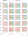 |
Fig. 8 Survival chart of a 1.0 MIo satellite for different satellite dissipations, from no dissipation (top row) to Δtsat = 1.0 Δt⊕ (bottom row), and for equilibrium tide only (Col. 1) and dynamical tide (Cols. 2-4) for different initial stellar rotation periods: 1 day (Cols. 1-2), 3 day (Col. 3) and 8 day (Col. 4). The fate of the satellites is a function of the disk lifetime (left vertical axis) and the corresponding final semimajor axis of the planet (right vertical axis) and its initial position (horizontal axis). The red and blue regions correspond to where the satellite is disrupted, and the green region to where it can survive. The black dashed line shows the final planet semimajor axis below which there is no survival of the satellites. The crossed-out area corresponds to cases where the planet itself falls onto the star. |
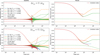 |
Fig. 9 Evolution of the semimajor axis of a 1.0 MIo satellite (left column) and its planet (right column) for different initial rotation periods of the star and two different satellite dissipations: 0 Δt⊕ (top row), and 0.1 Δt⊕ (bottom row). The disk lifetime is 35 000 yr, and the disk density 1000 g cm−2. |
5 What does this study teach us about the putative satellite around WASP-49 A b?
Given the results from our tidal migration simulations, we briefly examine the claim of a volcanic satellite orbiting the hot Saturn WASP-49 A b (Mp = 0.365 ± 0.019 MJup, Rp = 1.115 ± 0.047 RJup) at a putative orbital period of ~8 hours (~0.24 aIo), derived from variable alkali Doppler shift measurements (Oza et al. 2024). The range of allowed satellite periods for this system is estimated to be 6-12 hours (corresponding to 0.19-0.31 aIo), based on the stability criterion of the Hill Radius (~0.49 RHill following Domingos et al. 2006, and recently ~0.41 RHill from Kisare & Fabrycky 2024). This close-in orbit is compatible with a recent dynamical study considering planetary oblateness and stellar perturbations which showed a stability preference near (yet beyond) the Roche limit (Sucerquia & Cuello 2025). Satellite stability declines rapidly at larger satellite semimajor axes near the 1/2 Hill sphere criterion by Domingos et al. (2006); Kisare & Fabrycky (2024). The hot Saturn itself orbits its Sunlike star ( M⊙) at 2.79 days, which corresponds to a semimajor axis of ~ 0.039 AU.
This distance is similar to the shortest distance we consider in this study (0.035 AU), which is obtained when only considering the equilibrium tide in both star and planet (see Figures 7 and 8). The possible case of the putative satellite of WASP-49 A b is therefore more similar to our “equilibrium tide” case, for the shortest star-planet distance (i.e., longer disk lifetime) and the shortest planet-satellite distance. In these cases, regardless of satellite dissipation, we found that they do not survive the migration of the planet in the disk due to their proximity to the planet and the tides raised in the planet resulting in a tidal decay, which ultimately leads to engulfment.
Our system parameters differ slightly from those of WASP-49 A b. In particular, our Jupiter-like planet has a higher mass and a larger radius than the hot Saturn. This is important for two main reasons: for interactions with the disk and for tidal interactions. A less massive planet (0.365 ± 0.019 MJup) might not be able to open a gap in the circumstellar disk. A quick calculation following the Eq. (38) of Ida & Lin (2004) shows that a planet the mass of WASP-49 A b would open a gap in the disk for semimajor axes lower than 1.1 AU. Assuming the planet formed at distances higher than this value means that the circumplanetary disk was not isolated from the circumstellar disk and this could impact the formation of the satellite. If the planet was formed at distance lower than 1.1 AU, then the satellite might have formed in an isolated circumplanetary disk before the planet reaches our initial simulation distance of 0.15 AU. On the other hand, a larger planetary radius means a faster tidal evolution (all other parameters being equal). At an age of 1 Myr (our initial condition), our Jupiter has a radius of 1.48 RJup and at ~6 Myr (toward the end of the simulation), it remains around 1.41 RJup (Leconte & Chabrier 2013). This value is significantly larger than 1.115 RJup, the measured radius of WASP-49 A b (a value of 1.115 RJup corresponds to the modeled radius of a Jupiter-like planet at an age of about 140 Myr, Leconte & Chabrier 2013). As a result, the planetary tide we obtain in our simulations is stronger than in the present-day WASP-49 A system.
In any case, the formation of the system through type II migration of the host planet appears highly challenging. If the satellite’s orbit was confirmed, specific simulations should be conducted using the system’s parameters to explore why the planet may be less dissipative than expected (i.e., our assumed planetary Q might be too low, leading to an overestimated dissipation rate). In this work, we use a frequency-averaged tidal dissipation model (see Section 2.3.3). However, the actual dissipation of inertial waves exhibits a strong frequency dependence with peaks and troughs spanning several orders of magnitude (Ogilvie & Lin 2004). If the excitation frequency induced by the satellite coincides with a dissipation trough, the evolutionary timescale becomes significantly longer, and the satellite’s evolution would then be governed by the planet’s own evolution (as its radius contracts or as it spins up or down, shifting the locations of dissipation peaks and troughs, Ma & Fuller 2021). This could be investigated with the latest version of POSIDONIUS (Revol et al. 2024, Kwok et al., in prep., see next Section 6). Another possibility would be that the satellite was captured relatively “recently”, though this scenario seems unlikely given the planet’s close proximity to its host star.
Another scenario, recently discussed by Hansen (2023), involves the satellite becoming unbound. In our scenario, this would require both efficient outward migration and a highly dissipative satellite. Outward migration would facilitate the moon’s escape, while high dissipation would regulate eccentricity growth, preventing excessive values that could otherwise trigger dynamical disruption. In this case, the satellite could have formed, evolved, escaped the gravitational pull of the planet, only to later return and collide with the planet. However, it seems unlikely we are observing the satellite in the final stages of this process, as the timescale for such a collision must be short compared to the system’s age.
6 Conclusions
In this study, we investigated the survival of satellites of masses 1 MIo and 10 MIo during the migration of their host planet to close-in distances, typical for hot Jupiters. Our primary conclusion is that satellite survival becomes highly unlikely when the planet migrates closer than ≈0.1 AU. The key factors influencing satellite survival, in approximate order of importance, are (1) the final star-planet distance; (2) the initial satellite-planet distance; (3) the satellite’s tidal dissipation (where lower dissipation values increase survival rates); (4) the mass of the satellite (with more massive satellites exhibiting slightly higher survivability). Satellites that fail to survive are lost through two primary mechanisms: (1) dynamical disruption, where eccentricity excitations drives the satellite’s periastron below the Roche limit, and (2) tidal disruption, where orbital decay causes the satellite to gradually spiral inward until it reaches the Roche radius. Even for satellites that do survive the few million years of evolution modeled in our simulations, long-term stability is not guaranteed. This uncertainty is particularly relevant since we did not consider tidal dissipation values as high as Io’s (which is about 2.7 × Δt⊕), suggesting that our estimates are rather conservative. In reality, satellite survivability may be even lower than we predict here.
Ideally, studying the long-term survival of satellites would require significantly longer simulations, which are computationally expensive. As a result, our survival rates should be viewed as optimistic upper limits. As the system continues to evolve, the planet’s rotation gradually shifts toward pseudo-synchronization (consistent with the CTL model we adopted). The timescale for this evolution depends on the final star-planet distance, while the pseudo-synchronization period itself is determined by the planet’s semimajor axis and eccentricity (which remains very small throughout our simulations). Consequently, the corotation radius of the planet (which governs the direction of satellite migration) will continue to increase over time (as illustrated in Fig. 4, for instance). This implies that all the satellites positioned above the corotation radius at the end of our simulations will eventually migrate below it as the system evolves further. Once this transition occurs, both planetary tides and satellite tides (continuously driven by the eccentricity excitation caused by the nearby star) will work together to gradually decay the satellite’s orbit.
In this study we also explored the impact of the dynamical tide in both the star and the planet on 1) the evolution of the planet and 2) the evolution of the satellites it hosts. We identified several notable differences compared to cases where we considered only the equilibrium tide. In particular, massive satellites with high dissipation values (1 Δt⊕) failed to survive at starplanet distances smaller than 0.125 AU under the equilibrium tide model. This should remain true for even higher satellite dissipations. However, when dynamical tides were included, these dissipative satellites were more likely to persist; survival was possible around planets as close as 0.117 AU (for an initially slow-rotating star). This increased survival rate occurs because satellites that remain outside the corotation radius experience more efficient outward migration under the dynamical tide model compared to the equilibrium tide case. Given that the simulations including the dynamical tide are more realistic than the simulations with equilibrium tide only, this gives a small measure of hope for the survival of such satellites. We note, however, than the parameter space of surviving satellites is very narrow (they all start their evolution at 0.6 aIo, not closer to the planet or farther away).
Furthermore, our results suggest that the proposed satellite around WASP-49 A b is unlikely to have survived planetary migration unless specific conditions were met. Given the planet’s proximity to its host star and the typical tidal dissipation expected in gas giants, a satellite at the inferred orbital distance (~8 hours, ~0.24 aIo) would likely have been lost through tidal decay. This raises the possibility that the satellite, if real, was captured relatively recently or that the planet and the satellite have a significantly lower dissipation than assumed in our models. Further targeted simulations using WASP-49 A b’s specific system parameters would be necessary to assess this scenario in more detail.
Beyond extending the duration of our simulations, this study could be further improved by incorporating a fully consistent treatment of tides, as was recently implemented in Revol et al. (2024). POSIDONIUS very recently included the capability to model both the proper tidal response of the equilibrium tide in rocky bodies (allowed by Revol et al. 2024) and the frequencydependent dynamical tide response in gas giants and stars (Kwok et al., in prep.). These new advancements would allow us to revisit the evolution of our systems, and to incorporate the full tidal spectrum of a gas giant planet (Ogilvie & Lin 2004) or a star (Ogilvie & Lin 2007) along with the more chaotic migration it would induce in both planet and satellite (e.g., Auclair-Desrotour et al. 2014). In addition, they would offer a more consistent treatment of the eccentricity than we presented here (see discussion at the end of Section 2.3.2). This would allow us to explore the possibility that the satellite gets stuck in a trough of planetary dissipation, which then could help its survivability; at least with respect to the planetary dissipation, the satellite dissipation will always play a role, due to the eccentricity excitation raised by the close-in star. However, certain aspects of this improved tidal modeling (particularly for the dynamical tide in stars; Kwok et al. in prep.) are still under validation and development. Moreover, running simulations with these refinements enabled will require even greater computational resources and longer execution times than those required for this study. Thus, further investigation along these lines will be the focus of a future study.
A fully consistent treatment of tides as described in the previous paragraph would also allow us to investigate the evolution of multiple satellites around the planet, for which a correct treatment of the eccentric tides is even more relevant. Just as Jupiter’s inner satellites form a resonant chain (mean motion resonances), exomoons could also form such chains in which the eccentricity is excited to higher levels than in a nonresonant system. This eccentricity excitation would probably lead to a decrease in survivability of the satellites, especially that a new source of instabilities appear: satellite-satellite interactions and possible close-encounters. if we were to study this question, we would probably have to consider planets stopping migration farther away from the star than in this study (i.e., where the parameter space in initial planet-satellite distance is wider, see Fig. 8).
Additionally, we neglect here the tidal interaction between the star and the satellite. However, such an interaction might not be favorable for survival. Synchronization timescales are very similar when we consider the tide raised by the planet compared to the tide raised by the star on the satellite (calculated taking the orbital distance of the planet). This means that the two tides should be constantly fighting to synchronize the rotation of the satellite, which means that the satellite might never be synchronous with one or the other, which means then that there will always be some dissipation in the satellite. This nonsynchronization will enhance the inward migration due to the eccentricity of the satellite (see for instance Eq. (3) of Bolmont et al. 2011). To summarize, satellite survival during the inward migration of a hot Jupiter seems very challenging.
Data availability
For this work, we used POSIDONIUS version dbc5c8ec11e9055c0acfee91e012f39fe2fbc688 (https://www.blancocuaresma.com/s/posidonius). All initial conditions can be found on https://zenodo.org/records/14930048 as well as the internal structure file that includes the inverse values of the structural quality factor ( from Eq. (17)).
Acknowledgements
The authors would like to thank the anonymous referee for their constructive comments. This work was carried out within the framework of the NCCR PlanetS, supported by the Swiss National Science Foundation under grants 51NF40_182901 and 51NF40_205606. E.B. acknowledges the financial support of the SNSF (grant number: 200021_197176 and 200020_215760). C.M. acknowledges the support from the Swiss National Science Foundation under grant 200021_204847 “PlanetsInTime”. The research described in this paper was carried out in part at the Jet Propulsion Laboratory, California Institute of Technology, under a contract with the National Aeronautics Space Administration. © 2025. The computations were performed at University of Geneva on the Baobab and Yggdrasil clusters. This research has made use of the Astrophysics Data System, funded by NASA under Cooperative Agreement 80NSSC25M7105.
References
- Alibert, Y., Mordasini, C., Benz, W., & Winisdoerffer, C. 2005, A&A, 434, 343 [NASA ADS] [CrossRef] [EDP Sciences] [Google Scholar]
- Alibert, Y., Carron, F., Fortier, A., et al. 2013, A&A, 558, A109 [NASA ADS] [CrossRef] [EDP Sciences] [Google Scholar]
- Alvarado-Montes, J. A., Zuluaga, J. I., & Sucerquia, M. 2017, MNRAS, 471, 3019 [CrossRef] [Google Scholar]
- Auclair-Desrotour, P., Le Poncin-Lafitte, C., & Mathis, S. 2014, A&A, 561, L7 [NASA ADS] [CrossRef] [EDP Sciences] [Google Scholar]
- Aygün, B., & Cadek, O. 2024, Geophys. Res. Lett., 51, e2023GL107869 [Google Scholar]
- Barnes, J. W., & O’Brien, D. P. 2002, ApJ, 575, 1087 [NASA ADS] [CrossRef] [Google Scholar]
- Batygin, K., & Morbidelli, A. 2020, ApJ, 894, 143 [NASA ADS] [CrossRef] [Google Scholar]
- Batygin, K., Bodenheimer, P., & Laughlin, G. 2009, ApJ, 704, L49 [NASA ADS] [CrossRef] [Google Scholar]
- Batygin, K., Bodenheimer, P. H., & Laughlin, G. P. 2016, ApJ, 829, 114 [Google Scholar]
- Benisty, M., Bae, J., Facchini, S., et al. 2021, ApJ, 916, L2 [NASA ADS] [CrossRef] [Google Scholar]
- Blanco-Cuaresma, S., & Bolmont, E. 2017, in EWASS Special Session 4 (2017): Star-planet interactions (EWASS-SS4-2017) [Google Scholar]
- Bolmont, E., & Mathis, S. 2016, Celest. Mech. Dyn. Astron., 126, 275 [Google Scholar]
- Bolmont, E., Raymond, S. N., & Leconte, J. 2011, A&A, 535, A94 [NASA ADS] [CrossRef] [EDP Sciences] [Google Scholar]
- Bolmont, E., Selsis, F., Raymond, S. N., et al. 2013, A&A, 556, A17 [NASA ADS] [CrossRef] [EDP Sciences] [Google Scholar]
- Bolmont, E., Raymond, S. N., Leconte, J., Hersant, F., & Correia, A. C. M. 2015, A&A, 583, A116 [NASA ADS] [CrossRef] [EDP Sciences] [Google Scholar]
- Bolmont, E., Gallet, F., Mathis, S., et al. 2017, A&A, 604, A113 [NASA ADS] [CrossRef] [EDP Sciences] [Google Scholar]
- Bolmont, E., Demory, B. O., Blanco-Cuaresma, S., et al. 2020, A&A, 635, A117 [EDP Sciences] [Google Scholar]
- Canup, R. M., & Ward, W. R. 2002, AJ, 124, 3404 [Google Scholar]
- Cassidy, T. A., Mendez, R., Arras, P., Johnson, R. E., & Skrutskie, M. F. 2009, ApJ, 704, 1341 [Google Scholar]
- Crida, A., & Charnoz, S. 2012, Science, 338, 1196 [Google Scholar]
- Dhouib, H., Baruteau, C., Mathis, S., et al. 2024, A&A, 682, A85 [NASA ADS] [CrossRef] [EDP Sciences] [Google Scholar]
- Dobos, V., Charnoz, S., Pál, A., Roque-Bernard, A., & Szabó, G. M. 2021, PASP, 133, 094401 [NASA ADS] [CrossRef] [Google Scholar]
- Domingos, R. C., Winter, O. C., & Yokoyama, T. 2006, MNRAS, 373, 1227 [NASA ADS] [CrossRef] [Google Scholar]
- Eggleton, P. P., Kiseleva, L. G., & Hut, P. 1998, ApJ, 499, 853 [NASA ADS] [CrossRef] [Google Scholar]
- Fogg, M. J., & Nelson, R. P. 2007, A&A, 472, 1003 [NASA ADS] [CrossRef] [EDP Sciences] [Google Scholar]
- Gallet, F., Bolmont, E., Mathis, S., Charbonnel, C., & Amard, L. 2017, A&A, 604, A112 [NASA ADS] [CrossRef] [EDP Sciences] [Google Scholar]
- Gallet, F., Bolmont, E., Bouvier, J., Mathis, S., & Charbonnel, C. 2018, A&A, 619, A80 [NASA ADS] [CrossRef] [EDP Sciences] [Google Scholar]
- Gillon, M., Triaud, A. H. M. J., Demory, B.-O., et al. 2017, Nature, 542, 456 [NASA ADS] [CrossRef] [Google Scholar]
- Goldreich, P., & Nicholson, P. D. 1977, Icarus, 30, 301 [NASA ADS] [CrossRef] [Google Scholar]
- Gomes, G. O., Bolmont, E., & Blanco-Cuaresma, S. 2021, A&A, 651, A23 [NASA ADS] [CrossRef] [EDP Sciences] [Google Scholar]
- Guenel, M., Mathis, S., & Remus, F. 2014, A&A, 566, L9 [NASA ADS] [CrossRef] [EDP Sciences] [Google Scholar]
- Hansen, B. M. S. 2010, ApJ, 723, 285 [Google Scholar]
- Hansen, B. M. S. 2012, ApJ, 757, 6 [NASA ADS] [CrossRef] [Google Scholar]
- Hansen, B. M. S. 2023, MNRAS, 520, 761 [Google Scholar]
- Heller, R., & Hippke, M. 2024, Nat. Astron., 8, 193 [Google Scholar]
- Hut, P. 1981, A&A, 99, 126 [NASA ADS] [Google Scholar]
- Ida, S., & Lin, D. N. C. 2004, ApJ, 604, 388 [Google Scholar]
- Johnson, R. E., & Huggins, P. J. 2006, PASP, 118, 1136 [Google Scholar]
- Kaula, W. M. 1964, Rev. Geophys. Space Phys., 2, 661 [Google Scholar]
- Kipping, D. M. 2009, MNRAS, 392, 181 [NASA ADS] [CrossRef] [Google Scholar]
- Kipping, D., Bryson, S., Burke, C., et al. 2022, Nat. Astron., 6, 367 [NASA ADS] [CrossRef] [Google Scholar]
- Kisare, A. M., & Fabrycky, D. C. 2024, MNRAS, 527, 4371 [Google Scholar]
- Kreidberg, L., Luger, R., & Bedell, M. 2019, ApJ, 877, L15 [NASA ADS] [CrossRef] [Google Scholar]
- Lainey, V. 2016, Celest. Mech. Dyn. Astron., 126, 145 [NASA ADS] [CrossRef] [Google Scholar]
- Lainey, V., Arlot, J.-E., Karatekin, Ö., & van Hoolst, T. 2009, Nature, 459, 957 [Google Scholar]
- Leconte, J., & Chabrier, G. 2013, Nat. Geosci., 6, 347 [Google Scholar]
- Leconte, J., Chabrier, G., Baraffe, I., & Levrard, B. 2010, A&A, 516, A64 [NASA ADS] [CrossRef] [EDP Sciences] [Google Scholar]
- Lynden-Bell, D., & Pringle, J. E. 1974, MNRAS, 168, 603 [Google Scholar]
- Ma, L., & Fuller, J. 2021, ApJ, 918, 16 [NASA ADS] [CrossRef] [Google Scholar]
- Makarov, V. V., & Efroimsky, M. 2013, ApJ, 764, 27 [Google Scholar]
- Makarov, V. V., & Efroimsky, M. 2023, A&A, 672, A78 [NASA ADS] [CrossRef] [EDP Sciences] [Google Scholar]
- Mathis, S. 2015, A&A, 580, L3 [EDP Sciences] [Google Scholar]
- Mignard, F. 1979, Moon Planets, 20, 301 [Google Scholar]
- Mignard, F. 1981, MNRAS, 194, 365 [Google Scholar]
- Mordasini, C. 2018, Planetary Population Synthesis, 143 [Google Scholar]
- Mordasini, C., Alibert, Y., Benz, W., & Naef, D. 2009, A&A, 501, 1161 [NASA ADS] [CrossRef] [EDP Sciences] [Google Scholar]
- Neron de Surgy, O., & Laskar, J. 1997, A&A, 318, 975 [NASA ADS] [Google Scholar]
- Ogilvie, G. I. 2013, MNRAS, 429, 613 [Google Scholar]
- Ogilvie, G. I., & Lin, D. N. C. 2004, ApJ, 610, 477 [Google Scholar]
- Ogilvie, G. I., & Lin, D. N. C. 2007, ApJ, 661, 1180 [Google Scholar]
- Oza, A. V., Johnson, R. E., Lellouch, E., et al. 2019, ApJ, 885, 168 [Google Scholar]
- Oza, A. V., Seidel, J. V., Hoeijmakers, H. J., et al. 2024, ApJ, 973, L53 [NASA ADS] [CrossRef] [Google Scholar]
- Oza, A. V., Gebek, A., Westram, M. M. z., et al. 2025, MNRAS, accepted [arXiv:2509.08349] [Google Scholar]
- Park, R. S., Jacobson, R. A., Gomez Casajus, L., et al. 2025, Nature, 638, 69 [Google Scholar]
- Patel, S. D., Quarles, B., Cuntz, M., & Weinberg, N. N. 2025, MNRAS, 542, L144 [Google Scholar]
- Poon, M., Rein, H., & Pham, D. 2024, Open J. Astrophys., 7, 109 [Google Scholar]
- Quarles, B., Li, G., & Rosario-Franco, M. 2020, ApJ, 902, L20 [Google Scholar]
- Rein, H., & Spiegel, D. S. 2015, MNRAS, 446, 1424 [Google Scholar]
- Rein, H., & Tamayo, D. 2015, MNRAS, 452, 376 [Google Scholar]
- Revol, A., Bolmont, É., Sastre, M., et al. 2024, A&A, 691, L3 [NASA ADS] [CrossRef] [EDP Sciences] [Google Scholar]
- Ronnet, T., & Johansen, A. 2020, A&A, 633, A93 [NASA ADS] [CrossRef] [EDP Sciences] [Google Scholar]
- Saillenfest, M., Lari, G., & Boué, G. 2021, Nat. Astron., 5, 345 [NASA ADS] [CrossRef] [Google Scholar]
- Sartoretti, P., & Schneider, J. 1999, A&AS, 134, 553 [NASA ADS] [CrossRef] [EDP Sciences] [Google Scholar]
- Shakura, N. I., & Sunyaev, R. A. 1973, A&A, 500, 33 [NASA ADS] [Google Scholar]
- Spencer, J. R., Rathbun, J. A., Travis, L. D., et al. 2000, Science, 288, 1198 [NASA ADS] [CrossRef] [Google Scholar]
- Sucerquia, M., & Cuello, N. 2025, A&A, 694, L8 [NASA ADS] [CrossRef] [EDP Sciences] [Google Scholar]
- Teachey, A., & Kipping, D. M. 2018, Sci. Adv., 4, eaav1784 [Google Scholar]
- Trani, A. A., Hamers, A. S., Geller, A., & Spera, M. 2020, MNRAS, 499, 4195 [NASA ADS] [CrossRef] [Google Scholar]
- Unni, A., Oza, A. V., Hoeijmakers, H. J., et al. 2025, MNRAS, 540, L48 [Google Scholar]
- Wu, Y. 2005, ApJ, 635, 688 [Google Scholar]
- Zahn, J. P. 1975, A&A, 41, 329 [NASA ADS] [Google Scholar]
The dissipation in Io is also well characterized thanks to recent Doppler measurements by Juno (and Galileo): QIo = 11.4 ± 3.6 (Park et al. 2025).
For a comparison between the various values of dissipation we consider here and the typical tidal quality factor Qp, please refer to Appendix B.
This formulation allows the same computational implementation to handle both planetary and stellar dynamical tides.
Not all satellites are integrated until they either fall onto the star or reach 6 Myr. This is due to the fact that the closer the satellite the smaller the integration timestep. So for the cases where the fate is determined like the orange satellite, or where the integration to 6 Myr will not bring additional insights, we did not continue the integration.
For a comparison between the various dissipations considered here and the typical tidal quality factor Qsat, please refer to Appendix B.
Appendix A Validation of our implementation of the dynamical tide
Figure A.1 shows a comparison of POSIDONIUS simulations (ran for 10 Myr) compared to the Fig.6 of Bolmont et al. (2017). Our code reproduces well the behavior of Bolmont et al. (2017), in particular, we capture the change from dynamical tide to equilibrium tide regime visible in the 3 day case (in orange) at around 1 Myr of evolution. Due to the planet crossing the boundary corresponding to the frequency range of the excitation of the inertial waves (n = 2Ω*, where n is the orbital frequency and Ω* the stellar spin), the dissipation decreases from high values to much lower values slowing down quite significantly the inward migration. The planet then migrates inward following n = 2Ω* until it is so close to the star that the equilibrium tide itself is enough to drive the inward migration. This behavior is explained in more details in Bolmont et al. (2017). The slightly different timescales are thought to come from some differences of numerical values for some constants in the different codes. We note that for POSIDONIUS, the constants are referenced appropriately to ensure reproducibility whereas this was not done in Bolmont et al (2017)
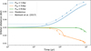 |
Fig. A.1 Comparison between the output of POSIDONIUS and Figure 6 in Bolmont et al. (2017) for the evolution of the semimajor axis of a Jupiter-mass planet, due to the dynamical tide and for different initial stellar rotation periods (1, 3, and 8 days). The dashed curves on this plot correspond to the cyan curves in Figure 6 in Bolmont et al. (2017), which were computed for a solar metallicity (Z = 0.0134). |
Appendix B A comparison between the various values of dissipation we consider and a tidal quality factor Q
In a generic case (i.e., when multiple frequencies are excited in the system), there is no obvious correspondence between Δt and a tidal quality factor Q or Q′ = 3/2 × Q/k2. The two models from which these parameters correspond (the Constant Time lag model for Δt and the Constant Phase lag for Q) are fundamentally incompatible (e.g., Leconte et al. 2010). However, a correspondence can be established if we restrict ourselves to a single excitation frequency. In the case of a purely circular coplanar orbit, this frequency is just 2|n - Ω| (semi-diurnal frequency), where n is the orbital frequency of the perturber and Ω the rotation frequency of the body in which the tides are operating. If n = Ω (i.e., the deformed primary body is synchronously rotating), then the dominant tidal mode is the eccentric annual mode with a frequency of n. Therefore, depending on whether we consider the planet or the satellite, the correspondence between a dissipation based on a Δt or a σ and a tidal quality factor Q is different.
B.1 For the planet
To compute a tidal quality factor Q′p for the planet corresponding to the equilibrium tide, the expression is
 (B.1)
(B.1)
 (B.2)
(B.2)
where nsat is the orbital frequency of the satellite and Ωp is the spin of the planet. In our simulations, the initial rotation period of the planet is 13 hr. We therefore calculate a value of Qp for the equilibrium tide of the planet with the value of σp given in the main text Section 2.3.3 for each initial satellite semimajor axis considered here. The values are given in Table B.1 for the initial age in our simulations (i.e., at an age of 106 yr) and toward the end of it (i.e., at an age of 6 × 10⁶ yr).
Values of the tidal quality factor Qp for the planet for the equilibrium tide and dynamical tide.
For the dynamical tide, we can directly compute the quality factor Q′p from the structural quality factor Q′s,p (of Eq. 17) as
 (B.3)
(B.3)
where  , as introduced in Sect. 2.3.3. Using the initial rotation period of the planet which is 13 hr, we can compute a Q′p, and if we take the value of k2 from the internal structure from Leconte & Chabrier (2013), we can compute a Qp. Table B.1 also gives these values (last column). As expected, the tidal quality factor for the dynamical tide is lower than for the equilibrium tide, which leads to faster evolution. However, our equilibrium tide tidal quality factor is lower than the high values proposed for the equilibrium tide in the introduction (Qp ~ 1010 − 1012, Goldreich & Nicholson 1977). Considering a lower value would impact our simulations for a nondissipative satellite; however, for realistic values of the satellite dissipation (Δtsat ~ 1 Δt⊕) the satellites’ fate is mainly due to satellite tide.
B.2 For the satellite
For the satellite, as its rotation very quickly evolves toward tidal locking (nsat = Ωsat), we cannot use Equation B.1. In that case, the main tidal mode is the eccentric annual mode of frequency n so that
 (B.4)
(B.4)
The values for the dissipation in the 1 MIo satellite are given in Table B.2. The values for Δtsat = 1.0 Δt⊕ are compatible with the recent values of Park et al. (2025) of QIo = 11.4 ± 3.6.
Values of the tidal quality factor Qsat for the satellites.
Appendix C Evolution of the planet’s rotation
Figure C.1 shows the evolution of the spin of the planet toward pseudo-synchronization for two different cases.
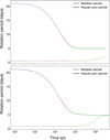 |
Fig. C.1 Rotation period of the planet (dashed lines) and pseudo-synchronization period (solid lines) as a function of time. The top panel corresponds to the simulation of Figure 4: τdisk = 3 × 10⁴ yr, 1 MIo, equilibrium tide only. The bottom panel corresponds to τdisk = 3 × 10⁴ yr, 1 MIo, initial stellar rotation of 8 day and the dynamical tide is on in both star and planet. The different colors correspond to the different satellite initial semimajor axes. They are all superimposed and the green one corresponds at an initial satellite semimajor axis of 0.6 aIo. |
The first one (top panel) corresponds to the simulation of Figure 4: τdisk = 3 × 10⁴ yr, 1 MIo, equilibrium tide only, while the second one (bottom panel) corresponds to: τdisk = 3 × 10⁴ yr, 1 MIo, dynamical tide in both star and planet and an initial stellar rotation of 8 day. In the first configuration, the planet stops its disk-induced migration at about 0.06 AU, while it stops at about 0.08 AU for the second.
In both cases, we see the pseudo-synchronization period (which is a function of the orbital frequency n of the planet and its eccentricity, here close to zero) sharply decreasing due to the disk-induced inward migration. It reaches a final value of about 5 days once the migration has stopped. The planet starts with a fast rotation (13 hours) and gradually slows down toward the pseudo-synchronization period.
In the top panel, the rotation of the planet does not reach the pseudo-synchronization period before the end of our simulation. In the bottom panel, the rotation of the planet evolves faster due to the enhanced dissipation in the planet due to the dynamical tide, and reaches pseudo-synchronization within 6 Myr.
Appendix D Impact of satellite mass for dynamical tide simulations
As discussed in Section 4.1.4, increasing the mass of the satellite reduces its susceptibility to dynamical disruption. This trend is evident when comparing Figures 8 and D.1, where the blue region (representing dynamically disrupted satellites) shrinks as satellite mass increases from 1 MIo to 10 MIo. For 1 MIo, dynamical disruption was still possible at 0.1 × Δt⊕, whereas for 10 MIo, only tidal disruption occurs. This distinction is further illustrated in Figure D.2, which presents examples of the orbital evolution for 1 MIo and 10 MIo satellites at Δtsat = 0.1 × Δt⊕, with an initial stellar rotation period of 1 day and varying disk lifetimes (corresponding to the second column and fourth row of Figs. 8 and D.1). In particular, Figure D.2d (bottom right panel), shows the evolution for the longest disk lifetime and a satellite initially located at 1 aIo. While the 1 MIo satellite undergoes dynamical disruption early in the evolution, the 10 MIo satellite experiences rapid eccentricity damping due to enhanced dissipation, leading to inward migration. Once the eccentricity is sufficiently damped, the inward migration slows down but then accelerates again when the satellite crosses the corotation radius, eventually reaching the Roche limit after a few 105 yr. This kind of evolution, predominantly governed by tides in the satellite, closely resembles the behavior observed in the equilibrium-tide only scenario (see Section 4.1.4).
Additionally, more massive satellites are less prone to tidal disruption, allowing them to survive around planets on closer orbits compared to their lower-mass counterparts. This effect is particularly evident for a dissipation of 0.1 Δt⊕ and for a satellite initially positioned farthest from the planet (1 aIo). This scenario still corresponds to the second column, fourth row of Figs. 8 and D.1. By comparing these two figures, we observe that 1 MIo satellites can only survive if the planet remains at a distance of ≥0.128 AU from the star. However, for 10 MIo satellites, survival is possible at slightly smaller separations, with the planet at ≥0.1097 AU from the star.
An example of orbital evolution for a disk lifetime of 1 × 10⁴ is shown in Figure D.2, which results in tidal disruption for the 1 MIo satellite (slight inward decay, orange cross in Fig. 8), but survival for the 10 MIo satellite (slight outward migration, light green cross in Fig. D.1). Similarly, Figure D.2b illustrates an evolution for a disk lifetime of 2 × 10⁴, leading to dynamical disruption for the 1 MIo satellite (blue cross in Fig. 8), but survival for the 10 MIo satellite (light green cross in Fig. D.1). In summary, Figure D.2 shows that 1 MIo satellites are either:
Dynamically disrupted for disk lifetimes ≥ 2 × 10⁴ yr (corresponding to star-planet distances ≤ 0.113 AU), or
Experience eccentricity excitation that gradually drives them toward the planet for disk lifetimes between 104 and 1.25 × 10⁴ yr (corresponding to star-planet distances 0.118 and 0.122 AU).
As discussed earlier, 10 MIo satellites can escape dynamical disruption for τdisk = 2, 3, 3.5×10⁴ yr by rapidly reducing their eccentricity due to the strong tide raised within them. Once their eccentricity has sufficiently decreased, they undergo strong planetary-tide induced outward migration, which allows them to survive. This strong outward migration also prevents their orbit from slowly decaying, particularly for disk lifetimes between 104 and 1.25 × 10⁴ yr.
As with the 1 MIo satellite, the initial stellar rotation has a minimal impact on survival. While variations exist for a given disk lifetime, a more consistent pattern emerges when focusing instead on the planet’s final distance from the star. Although more massive satellites survive around planets which are closer to their star than their 1 MIo counterparts, the overall limit remains of the same order of magnitude between the two masses. Satellites closer than 0.1 AU are unlikely to survive. The increased survivability of massive satellites is primarily due to efficient outward migration induced by the planetary tide (as seen in Fig. D.2b and c) when they remain outside corotation. However, this also means that their eccentricity becomes more excited as they approach the Hill radius, eventually leading to a slow tidal decay when: 1) the planetary tide weakens as the planet’s radius decreases over time, 2) the corotation radius increases sufficiently to reverse the planetary tide-driven migration. Thus, our survival rates should be regarded as optimistic upper limits.
For the 10 MIo satellites, the effect of the initial stellar rotation is slightly more pronounced compared to 1 MIo satellites. This distinction is particularly noticeable at the high satellite dissipation (last row of Fig. D.1). This indicates that for initially slow-rotating stars, the survival limit can shift slightly inward. Specifically, for an initial stellar rotation period of 1 day, while the satellite survives only if the planet remains beyond 0.122 AU, it does not persist at 0.118 AU. However, for a slower initial stellar rotation period of 8 days, the satellite survives at slightly smaller orbital separations, remaining stable as long as the planet is beyond 0.117 AU. Nevertheless, the overall effect remains small.
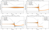 |
Fig. D.2 Evolution of the semimajor axis of a 1.0 MIo and a 10 MIo satellite on initially wide orbits for different disk lifetimes (i.e., different final planet distances). For all these cases, the initial rotation of the star is 1 day and the dissipation is Δtsat = 0.1 Δt⊕ (which corresponds to the Col. 2, fourth row of Figs. 8 and D.1): (a) τdisk = 1 × 10⁴ yr, asat,i = 1.0 aIo; (b) τdisk = 2 × 10⁴ yr, asat,i = 1.0 aIo; (c) τdisk = 3.5 × 10⁴ yr, asat,i = 0.8 aIo; (d) τdisk = 5 × 10⁴ yr, asat,i = 1.0 aIo. These combinations were chosen to highlight some behaviors. |
All Tables
Values of the tidal quality factor Qp for the planet for the equilibrium tide and dynamical tide.
All Figures
|
Fig. 1 Schema of the simulation setup. An Io-like satellite orbits around a Jupiter-like planet with a solar-like host star. |
| In the text | |
|
Fig. 2 Evolution of the disk surface density Σg(r, t). |
| In the text | |
|
Fig. 3 Evolution of the semimajor axis and eccentricity of a Jupiter-mass planet due to type II migration for different disk lifetimes τdisk and different assumptions on the stellar tide. The dashed lines correspond to the case where only the equilibrium tide in the star is accounted for; the solid lines correspond to cases where both the equilibrium tide and dynamical tide are taken into account (initial fast stellar rotation period of 1 day). We note that the rotation of the star is evolving, here mainly due to the contraction of the radius, and its evolution is encoded in the corotation radius curve (i.e., where the orbital frequency is equal to the stellar spin). For clarity, we only plot two cases in the bottom panel (τdisk = 2 × 10⁴ yr and 5 × 10⁴ yr). The equilibrium tide is still represented with dashed lines, but also with transparency to ease identification. |
| In the text | |
|
Fig. 4 Evolution of a 1 MIo satellite orbiting a migrating Jupiter-mass planet for different initial distances of the satellite. Here the disk lifetime is 3 × 10⁴ yr, the initial rotation period of the star is 1 day and the dissipation in the satellite is taken to be 0. The top left panel shows the evolution of the semimajor axis of the satellite (solid colored lines); the shaded colored lines represent the periastron and apoastron. The gray dotted line represents the radius of the planet, the black dash-dotted line represents the Roche radius, the black dashed line the corotation radius (where the satellite’s mean motion is equal to the spin of the planet), and the gray dashed line represents one-half of the Hill radius of the planet. The bottom left panel shows the evolution of the satellite’s eccentricity. The top right panel shows the evolution of the semimajor axis of the planet (solid colored lines). The black dashed line represents the corotation radius (where the planet’s mean motion is equal to the spin of the star). The bottom left panel shows the evolution of the planet’s eccentricity. |
| In the text | |
|
Fig. 5 Same as the right column of Figure 4, but for a disk lifetime of 5 × 10³ yr (left column) and 5 × 10⁴ yr (right column). The top row shows the evolution of the orbital distance of the satellites and the bottom row shows the evolution of their eccentricities. For the left column, the final semimajor axis of the planet is 0.125 AU and for the right column, it is 0.035 AU. This difference can be visualized thanks to the gray dashed lines corresponding to one-half of the Hill radius of the planet, which comes much closer to the planet when the τdisk = 5 × 10⁴ yr. |
| In the text | |
|
Fig. 6 Evolution of the semimajor axis and eccentricity (through apoastron and periastron distances) of a 1.0 MIo satellite for different satellite dissipations. Here the disk lifetime is 35 000 yr, and the disk density 1000 g cm−2. The evolution is shown for two different initial satellite semimajor axes: 0.4 aIo (top panel) and 0.6 aIo (bottom panel). |
| In the text | |
|
Fig. 7 Survival chart of a 1.0 MIo (first row) and a 10.0 MIo (second row) satellite for different satellite dissipations and for equilibrium tides only, from no dissipation (left) to Δtsat = 1 Δt⊕ (right). The fate of the satellites is a function of the disk lifetime (left vertical axis) and the corresponding final semimajor axis of the planet (right vertical axis) and its initial position (horizontal axis). The blue crosses and region correspond to the dynamical disruption scenario. The red crosses correspond to satellites that underwent a tidal disruption within the simulation time (5 Myr), the orange crosses correspond to satellites that are migrating inward at a rate faster than 10−4 AU/Myr. This population (red and orange crosses) is outlined by the red region. The dark green check signs correspond to satellites whose fate is not clear (migration lower than 10−4 AU/Myr). The light green check signs correspond to an outward migration at a rate faster than 10−4 AU/Myr. The green region therefore corresponds to satellites that should survive. The black dashed line shows the final planet semimajor axis below which there is no survival of satellites. |
| In the text | |
|
Fig. 8 Survival chart of a 1.0 MIo satellite for different satellite dissipations, from no dissipation (top row) to Δtsat = 1.0 Δt⊕ (bottom row), and for equilibrium tide only (Col. 1) and dynamical tide (Cols. 2-4) for different initial stellar rotation periods: 1 day (Cols. 1-2), 3 day (Col. 3) and 8 day (Col. 4). The fate of the satellites is a function of the disk lifetime (left vertical axis) and the corresponding final semimajor axis of the planet (right vertical axis) and its initial position (horizontal axis). The red and blue regions correspond to where the satellite is disrupted, and the green region to where it can survive. The black dashed line shows the final planet semimajor axis below which there is no survival of the satellites. The crossed-out area corresponds to cases where the planet itself falls onto the star. |
| In the text | |
|
Fig. 9 Evolution of the semimajor axis of a 1.0 MIo satellite (left column) and its planet (right column) for different initial rotation periods of the star and two different satellite dissipations: 0 Δt⊕ (top row), and 0.1 Δt⊕ (bottom row). The disk lifetime is 35 000 yr, and the disk density 1000 g cm−2. |
| In the text | |
|
Fig. A.1 Comparison between the output of POSIDONIUS and Figure 6 in Bolmont et al. (2017) for the evolution of the semimajor axis of a Jupiter-mass planet, due to the dynamical tide and for different initial stellar rotation periods (1, 3, and 8 days). The dashed curves on this plot correspond to the cyan curves in Figure 6 in Bolmont et al. (2017), which were computed for a solar metallicity (Z = 0.0134). |
| In the text | |
|
Fig. C.1 Rotation period of the planet (dashed lines) and pseudo-synchronization period (solid lines) as a function of time. The top panel corresponds to the simulation of Figure 4: τdisk = 3 × 10⁴ yr, 1 MIo, equilibrium tide only. The bottom panel corresponds to τdisk = 3 × 10⁴ yr, 1 MIo, initial stellar rotation of 8 day and the dynamical tide is on in both star and planet. The different colors correspond to the different satellite initial semimajor axes. They are all superimposed and the green one corresponds at an initial satellite semimajor axis of 0.6 aIo. |
| In the text | |
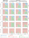 |
Fig. D.1 Same as Figure 8, but for a satellite of 10 MIo. |
| In the text | |
|
Fig. D.2 Evolution of the semimajor axis of a 1.0 MIo and a 10 MIo satellite on initially wide orbits for different disk lifetimes (i.e., different final planet distances). For all these cases, the initial rotation of the star is 1 day and the dissipation is Δtsat = 0.1 Δt⊕ (which corresponds to the Col. 2, fourth row of Figs. 8 and D.1): (a) τdisk = 1 × 10⁴ yr, asat,i = 1.0 aIo; (b) τdisk = 2 × 10⁴ yr, asat,i = 1.0 aIo; (c) τdisk = 3.5 × 10⁴ yr, asat,i = 0.8 aIo; (d) τdisk = 5 × 10⁴ yr, asat,i = 1.0 aIo. These combinations were chosen to highlight some behaviors. |
| In the text | |
Current usage metrics show cumulative count of Article Views (full-text article views including HTML views, PDF and ePub downloads, according to the available data) and Abstracts Views on Vision4Press platform.
Data correspond to usage on the plateform after 2015. The current usage metrics is available 48-96 hours after online publication and is updated daily on week days.
Initial download of the metrics may take a while.