| Issue |
A&A
Volume 704, December 2025
|
|
|---|---|---|
| Article Number | A164 | |
| Number of page(s) | 15 | |
| Section | Interstellar and circumstellar matter | |
| DOI | https://doi.org/10.1051/0004-6361/202555037 | |
| Published online | 15 December 2025 | |
Anisotropy in the carbon monoxide (CO) line emission across the Milky Way’s disk
1
Istituto di Astrofisica e Planetologia Spaziali (IAPS). INAF.
Via Fosso del Cavaliere 100,
00133
Roma,
Italy
2
Department of Astronomy, University of Massachusetts,
Amherst,
MA
01003,
USA
3
Laboratoire AIM, Paris-Saclay, CEA/IRFU/SAp – CNRS – Université Paris Diderot,
91191
Gif-sur-Yvette Cedex,
France
4
Universität Heidelberg, Zentrum für Astronomie, Institut für Theoretische Astrophysik,
Albert-Ueberle-Str. 2,
69120
Heidelberg,
Germany
5
Universität Heidelberg, Interdiszipliäres Zentrum für Wissenschaftliches Rechnen,
Im Neuenheimer Feld 225,
69120
Heidelberg,
Germany
6
Harvard-Smithsonian Center for Astrophysics,
60 Garden Street,
Cambridge,
MA
02138,
USA
7
Elizabeth S. and Richard M. Cashin Fellow at the Radcliffe Institute for Advanced Studies at Harvard University,
10 Garden Street,
Cambridge,
MA
02138,
USA
8
Dipartimento di Fisica, Università di Roma Tor Vergata,
Via della Ricerca Scientifica 1,
00133
Roma,
Italy
9
SUPA, School of Physics and Astronomy, University of St Andrews,
North Haugh,
St Andrews
KY16 9SS,
UK
10
École Polytechnique Fédérale de Lausanne, Observatoire de Sauverny,
Chemin Pegasi 51,
1290
Versoix,
Switzerland
★ Corresponding author: This email address is being protected from spambots. You need JavaScript enabled to view it.
Received:
4
April
2025
Accepted:
14
September
2025
Abstract
We present a study of the CO line emission anisotropy across the Milky Way’s disk to examine the effect of stellar feedback and Galactic dynamics on the distribution of the dense interstellar medium. We used the Hessian matrix method to characterize the 12CO(1–0) line emission distribution and identify the preferential orientation across line-of-sight velocity channels in the Dame et al. (2001, ApJ, 547, 792) composite Galactic plane survey, which covers the Galactic latitude range |b| < 5°. The structures sampled with this tracer are predominantly parallel to the Galactic plane toward the inner Galaxy, in clear contrast to the predominantly perpendicular orientation of the structures traced by neutral atomic hydrogen (HI) emission toward the same regions. The analysis of the Galactic plane portions sampled at higher angular resolution with other surveys reveals that the alignment with the Galactic plane is also prevalent at smaller scales. We find no preferential orientation in the CO emission toward the outer Galaxy, in contrast to the preferential alignment with the Galactic plane displayed by HI in that portion of the Milky Way. We interpret these results as the combined effect of the decrease in midplane pressure with increasing Galactocentric radius and SN feedback, which lifts diffuse gas more efficiently than dense gas off the Galactic plane.
Key words: ISM: clouds / ISM: general / ISM: kinematics and dynamics / ISM: structure / Galaxy: structure
© The Authors 2025
 Open Access article, published by EDP Sciences, under the terms of the Creative Commons Attribution License (https://creativecommons.org/licenses/by/4.0), which permits unrestricted use, distribution, and reproduction in any medium, provided the original work is properly cited.
This article is published in open access under the Subscribe to Open model. This email address is being protected from spambots. You need JavaScript enabled to view it. to support open access publication.
1 Introduction
Carbon monoxide (CO) emission is a crucial tracer of the cold, dense gas associated with star formation (Kennicutt & Evans 2012; Heyer & Dame 2015). Molecular clouds (MCs) traced by CO have been extensively sampled in the Milky Way and nearby galaxies (see, for example, Fukui & Kawamura 2010; Heyer & Dame 2015; Schinnerer & Leroy 2024). However, many aspects of the MC life cycle remain uncertain. For example, the impact of stellar winds, radiation, and supernovae (SNe) interacting with the surrounding gas on different scales, and the role of this interaction in the formation and dissipation of MCs, have not yet been established (see, for example, Elmegreen 2000; Krumholz et al. 2014; Klessen & Glover 2016; Mac Low et al. 2017). In this paper, we investigate the Galactic processes that influence the MC life cycle by studying the anisotropy in the CO line emission distribution throughout the Galactic plane, extending the study of neutral atomic hydrogen (HI) emission presented in Soler et al. (2022) to the molecular gas phase.
High star formation rate (SFR) densities can produce sufficient energy and momentum to launch outflows of ionized, neutral, and molecular gas that can potentially escape the main body of a galaxy (see, for example, Dekel & Silk 1986; Krumholz et al. 2017). These galactic outflows remove the raw material for future star formation, enriching the galactic disk and circumgalactic medium with heavy metals and thereby driving the evolution of galaxies (see, for example, Veilleux et al. 2005; Fabian 2012; Saintonge & Catinella 2022). Starburst-driven molecular winds have been observed in emission stacks of nearby ultraluminous infrared galaxies (see, for example, Chung et al. 2011). They are resolved near the disks of local starburst galaxies, such as NGC253 (d = 3.5 Mpc; Sakamoto et al. 2006; Bolatto et al. 2013; Krieger et al. 2019), M82 (d = 3.9 Mpc; Weiß et al. 1999; Walter et al. 2002; Matsushita et al. 2005; Leroy et al. 2015), NGC1808 (d = 10.8 Mpc; Salak et al. 2018), NGC2146 (d = 17.2 Mpc; Tsai et al. 2009; Kreckel et al. 2014), NGC3256 (d = 35 Mpc; Sakamoto et al. 2006), and ESO320-G030 (d = 48 Mpc; Pereira-Santaella et al. 2016). Stuber et al. (2021) report that almost a quarter of the 90 nearby main-sequence galaxies covered in the Physics at High Angular resolution in Nearby GalaxieS (PHANGS) ALMA Survey show evidence of central molecular winds.
The mean SFR in these starburst galaxies exceeds that of the Milky Way by at least two orders of magnitude (Elia et al. 2022; Zari et al. 2023; Soler et al. 2023; Elia et al. 2025). However, the Galactic SFR may induce weaker outflows that shape the molecular gas and drive metallicity changes throughout the Galactic disk (see, for example, Hayward & Hopkins 2017; Kim & Ostriker 2018; Sharda et al. 2024). Studies of blown-out molecular structures in the Milky Way have been limited to the central region of the Galaxy (see, for example, Di Teodoro et al. 2020; Heyer et al. 2025). A systematic study of their prevalence throughout the disk is not yet available.
Soler et al. (2022) used a morphological decomposition in terms of filaments to study the anisotropy in the HI emission toward the Milky Way’s disk using the 16.′2-resolution observations in the HI 4π (HI4PI) survey (HI4PI Collaboration 2016). Their study identifies a transition in the preferential orientation of the HI filamentary structures with Galactocentric radius, from mostly perpendicular or with no preferred orientation relative to the Galactic plane for Galactocentric radii Rgal < 10 kpc to mostly parallel for Rgal > 10 kpc. By comparison with the populations of high-mass stars and identified SN bubbles, as well as the results obtained in numerical magnetohydrodynamic (MHD) simulations of a multiphase stratified Galactic medium, the authors interpret this result as the imprint of SN feedback in the inner Galaxy and of Galactic rotation and shear in the outer Milky Way (Soler et al. 2020). In this paper, we apply the method introduced in Soler et al. (2022) to study the anisotropy in the distribution of CO emission across the Galactic plane and to identify the prevalence of vertical molecular structures that may indicate molecular galactic outflows.
Extended surveys of CO emission toward the Galactic plane have enabled the discovery of long, high-density filamentary features that could be shaped by the structural dynamics of the Milky Way, such as the Nessie cloud (Goodman et al. 2014). These objects, typically associated with filamentary infrared dark clouds (IRDCs), have been identified and cataloged using a variety of methods (see, for example, Ragan et al. 2014; Abreu-Vicente et al. 2016; Wang et al. 2016). Their lengths range between tens and a few hundred parsecs, their masses between 103 and 106 M⊙, and their aspect ratios between 3:1 and 117:1; they are preferentially oriented parallel to the Galactic plane (Zucker et al. 2018). More recently, Neralwar et al. (2022a) and Neralwar et al. (2022b) employed a combination of visual analysis and J-plots classification (Jaffa et al. 2018) to study the morphology of clouds in the 12CO(2–1) line emission observations in the Structure, Excitation and Dynamics of the Inner Galactic Interstellar Medium (SEDIGISM) survey (Schuller et al. 2021). The authors found that most clouds sampled with that tracer are elongated, but did not quantify their prevalent orientation.
This work focuses on the preferential orientation of filamentary structures in CO emission to identify trends across line-of-sight (LOS) velocities (vLSR). Thus, we do not consider the physical properties of individual filamentary structures, recently reviewed in Hacar et al. (2023), but rather the orientation of high-aspect-ratio features in the emission as a marker of anisotropy in the velocity field. Such a study has never been performed in CO across the Galactic plane, using circular statistics tools to quantify the emission anisotropy.
This paper is organized as follows. Section 2 presents the CO observations used in this study. In Sect. 3, we introduce the Hessian matrix method to identify filamentary structures and the circular statistics employed to quantify its anisotropy. Sect. 4 describes the global trends in CO anisotropy and its relation with the HI emission. We discuss the implications of these results for our understanding of the Galactic structure in Sect. 5. Finally, in Sect. 6, we present our conclusions. We complement the main results of this work with additional analyses in a set of appendices. Appendix A presents details on the Hessian method’s error propagation and selection of parameters. In Appendix B, we show that the reported filament anisotropy in CO emission can also be recovered using the preferential orientation of intensity gradients. We present a study of synthetic emission maps generated using fractional Brownian motion (fBm) realizations in Appendix C, which we used to illustrate the effects of beam size on the Hessian analysis results.
2 Data
Carbon monoxide (CO) emission surveys do not uniformly cover the Galactic plane (see, for example, Heyer & Dame 2015). The highest angular-resolution survey of CO line emission covering the whole Galactic plane with the same isotopologue and transition is the 12CO(1–0) compilation presented by Dame et al. (2001). That is the core dataset used in this analysis.
We also included other surveys to extend our study to higher (sub-arcminute) angular resolutions for selected regions of the Galactic plane. First, we examined the Milky Way Imaging Scroll Painting (MWISP) survey, which sampled the 12CO(1–0), 13CO(J=1–0), and C18O (J=1–0) line emission toward the Galactic plane and has so far released observations for the region within |b| < 1°for 25.°0 < l < 49.°0. Second, we considered the Forgotten Quadrant Survey (FQS; Benedettini et al. 2020), which sampled the 12CO(1–0) line emission in the range 220° < l < 240° and −2°.5 < b < 0°.
We acknowledge other higher-resolution 12CO(1–0) surveys covering different portions of the plane, for example, the FOREST Unbiased Galactic plane Imaging Survey with the Nobeyama 45-m telescope (FUGIN; Umemoto et al. 2017) and the Census of High- and Medium-mass Protostars (CHaMP) survey (Barnes et al. 2016). However, our goal is to illustrate examples of the reported 12CO(1–0) anisotropies at higher resolutions, rather than to produce a global anisotropy analysis at higher resolutions, which would require the combination of a diverse set of datasets beyond the scope of this work.
2.1 The Dame et al. (2001) composite CO survey of the Milky Way disk
The 12CO(1–0) line emission observations presented by Dame et al. (2001) encompass the surveys obtained over two decades with the Harvard-Smithsonian Center for Astrophysics (CfA) 1.2-m telescope and a similar instrument at Cerro Tololo in Chile. These observations have an angular resolution of 8.′5 at 115 GHz, corresponding to the frequency of the 12CO(1–0) line.
For this study, we used the interpolated composite Galactic plane survey, which covers the range 0.0 < l < 360.0° and |b| ≤ 5° with 1.3-km s−1-wide spectral channels. The noise level through-out this dataset is not uniform, as it combines surveys with different instruments and was acquired at various times. The standard noise level estimation for this dataset is discussed in appendix A of Miville-Deschênes et al. (2017), with the authors identifying three peaks in the noise distribution at 0.06, 0.10, and 0.19K per channel. We adopted the highest of these values, 0.19K per channel, as the global noise level for this dataset.
We used the astropy reproject package to project these data onto a spatial grid covering 0.°0 < l < 360.°0 and |b| < 5°.0 with a pixel size ∆l = ∆b =7.′5. We also used the astropy spectral-cube package to project the spectral axis of these observations onto the 1.29-km s−1-resolution spectral grid of the HI4PI survey (HI4PI Collaboration 2016). This spectral repro-jection enables direct comparison with the results presented by Soler et al. (2022) and does not significantly alter the results of our analysis.
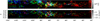 |
Fig. 1 Example of 12CO(1–0) line emission intensity (top) and the corresponding filamentary structures identified using the Hessian matrix method (bottom) toward a portion of the Galactic plane. The map shown in each color corresponds to the emission in a 1.29-km s−1-wide channel centered on the line-of-sight velocity indicated on the left-hand side of the top panel. |
2.2 The Milky Way Imaging Scroll Painting (MWISP) survey
The MWISP project is a high-sensitivity survey of the northern Galactic plane conducted with the Purple Mountain Observatory 13.7-m telescope (Sun et al. 2018; Su et al. 2019). It comprises the 12CO(1–0), 13CO(1–0), and C18O (1–0) lines simultaneously observed by the nine-beam Superconducting Spectroscopic ARray (SSAR) receiver system (Shan et al. 2012). The full-width half maximum (FWHM) of the observations is 49′′ at the 12CO frequency and 51′′ at the 13CO and C18O frequencies.
The SSAR bandwidth of 1 GHz with 16 384 channels provides a velocity coverage of 260 km s−1 and a spectral resolution of 61 kHz, equivalent to velocity separations of about 0.16 km s−1 for 12CO and 0.17 km s−1 for 13CO and C18O. This velocity range enables the sampling of vLSR < 0 km s−1 toward the first Galactic quadrant (QI), which is excluded in other high-resolution CO surveys of the Galactic plane, such as the Boston University-Five College Radio Astronomy Observatory Galactic Ring Survey (GRS; Jackson et al. 2006) and FUGIN (Umemoto et al. 2017). The typical MWISP root-mean-square (RMS) noise levels are about 0.5 K for 12CO and 0.3 K for 13CO and C18O. The final data products are position-position-velocity (PPV) cubes constructed from mosaics with a spatial grid spacing of 30′′.
2.3 The Forgotten Quadrant Survey (FQS)
The FQS is based on 700 hours of observations with the Arizona Radio Observatory (ARO) 12-m antenna. It covered the Galactic plane in the range 220° < l < 240°and −2.°5 < b < 0° sampling the 12CO(1–0) and 13CO(1–0) emission. The survey was divided into partially overlapping 30′ × 30′ tiles with sides aligned along the Galactic longitude and latitude. Each tile was observed twice in the on-the-fly observing mode, scanning in mutually orthogonal directions: one along l and one along b. The angular resolution of these observations is determined by the 55′′ telescope beam at 115 GHz. The data were acquired by scanning rows separated by 18′′. The FQS 12CO(1–0) data products are distributed on a grid with 17.′′3 pixels and 0.65-km s−1-wide velocity channels. We employed the FQS observations resam-pled to a spectral resolution of 1.0-km s−1, for which the RMS noise level has a median value of 0.53 K. Further details of data acquisition and reduction information is presented in Benedettini et al. (2020).
3 Methods
We applied the Hessian matrix method for filament identification as follows. We considered CO line emission maps across velocity channels ICO(l, b, vLSR), where the position in the sky is given by the Galactic longitude and latitude, l and b, and vLSR is the line-of-sight velocity with respect to the local standard of rest (LSR). For each vLSR channel, we estimated the derivatives with respect to the local coordinates (x, y) and built the Hessian matrix,
![Mathematical equation: ${\bf{H}}(x,y) \equiv \left[ {\matrix{ {{H_{xx}}} \hfill & {{H_{xy}}} \hfill \cr {{H_{yx}}} \hfill & {{H_{yy}}} \hfill \cr } } \right],$](/articles/aa/full_html/2025/12/aa55037-25/aa55037-25-eq1.png) (1)
where Hxx ≡ ∂2 I/∂x2, Hxy ≡ ∂2 I/∂x∂y, Hyx ≡ ∂2 I/∂y∂x, Hyy ≡ ∂2 I/∂y2, and x and y are related to the Galactic coordinates (l, b) as x ≡ l cos b and y ≡ b, so that the x axis is parallel to the Galactic plane. In the sky areas considered in this study, |b| ≤ 5°, cos b ≈ 1, so the derivatives were performed on a tangent-plane projection of each tile, where x ≡ l and y ≡ b.
(1)
where Hxx ≡ ∂2 I/∂x2, Hxy ≡ ∂2 I/∂x∂y, Hyx ≡ ∂2 I/∂y∂x, Hyy ≡ ∂2 I/∂y2, and x and y are related to the Galactic coordinates (l, b) as x ≡ l cos b and y ≡ b, so that the x axis is parallel to the Galactic plane. In the sky areas considered in this study, |b| ≤ 5°, cos b ≈ 1, so the derivatives were performed on a tangent-plane projection of each tile, where x ≡ l and y ≡ b.
We obtained the partial spatial derivatives using Gaussian derivatives, that is, by convolving I(l, b, v) with the second derivatives of a two-dimensional Gaussian function, following the procedure described in Soler et al. (2013). To match the angular scales considered in Soler et al. (2022), we employed an 18′ FWHM derivative kernel. Results obtained with different derivative kernel sizes are presented in Appendix A.
We computed the eigenvalues (λ±) of the Hessian matrix using the characteristic equation,
 (2)
(2)
These eigenvalues characterize the local curvature of the intensity (see, for example, Frangi et al. 1998; Pogosyan et al. 2009; Schisano et al. 2020). The largest |λ±| corresponds to the largest curvature direction of the scalar field. If for a particular point, λ+ <0 and λ− <0, the curvature of the is convex, thus corresponding to a ridge or a peak. Given that λ+ > λ− in Eq. (2) and both are negative along a convex structure, λ− corresponds to the direction of the largest curvature direction, thus highlighting ridges in the scalar field, as illustrated in Fig. 1. For those elongated structures, λ+ corresponds to the field curvature along the ridge.
The Hessian matrix also provides the orientation of the intensity ridges with respect to the Galactic plane through the angle
![Mathematical equation: $\theta = {1 \over 2}\arctan \left[ {{{{H_{xy}} + {H_{yx}}} \over {{H_{xx}} - {H_{yy}}}}} \right].$](/articles/aa/full_html/2025/12/aa55037-25/aa55037-25-eq3.png) (3)
(3)
We estimated an angle, θij, for each of the m × n pixels in a velocity channel map, where the indices i and j run over the pixels along the x and y axes, respectively. However, this angle is only meaningful in regions of the map classified as filamentary according to selection criteria based on the values of λ− and the noise properties of the data (see, for example, Planck Collaboration Int. XXXII 2016).
We conducted the Hessian analysis in 10° × 10° tiles across velocity channels. We selected the filamentary structures in each tile according to the criterion λ− < 0. Additionally, we selected regions where I(l, b, v) > 3σI, with σ1 corresponding to the RMS noise presented in Sect. 2. Following the method introduced in Planck Collaboration Int. XXXII (2016), we further selected filamentary structures based on the values of the eigenvalue λ− in noise-dominated data portions. We estimated λ− in five velocity channels with low signal-to-noise ratios (S/N) and determined the minimum value of λ in each. We used the median of these five λ− values as the threshold value,  . The median was used to reduce the influence of outliers. In general, the values of λ− in the noise-dominated channels are similar, and this selection does not imply any loss of generality. We considered only regions of each velocity channel map where
  , corresponding to filamentary structures with curvatures in I(l, b, v) larger than those in the noise-dominated channels.
Once the filamentary structures were selected, we used the angles derived from Eq. (3) to study their orientation relative to the Galactic plane. To systematically evaluate the preferential orientation, we applied the projected Rayleigh statistic (V) (see, for example, Batschelet 1981), which is a test to determine whether the distribution of angles is nonuniform and peaks at a particular angle. This test is equivalent to the modified Rayleigh test for uniformity proposed by Durand & Greenwood (1958) for the specific directions of interest θ = 0° and 90° (Jow et al. 2018), such that V > 0 or V < 0 correspond to preferential orientations parallel or perpendicular to the Galactic plane, respectively. It is defined as
 (4)
where the indices i and j run over the pixel locations in the two spatial dimensions (l, b) for a given velocity channel and wij is the statistical weight of each angle θij.
(4)
where the indices i and j run over the pixel locations in the two spatial dimensions (l, b) for a given velocity channel and wij is the statistical weight of each angle θij.
The values of V indicate significance only if sufficient clustering is found around the orientations θ = 0°, and 90°. The null hypothesis implied in V is that the angle distribution is uniform or centered on a different orientation. In the case of independent and uniformly distributed angles, and for a large number of samples, values of V ≈ 1.64 and 2.57 correspond to rejecting the null hypothesis with probabilities of 5% and 0.5%, respectively (Batschelet 1972). A value of |V| ≈ 2.87 is approximately equivalent to a 3σ confidence interval. We present our analysis results in terms of the mean orientation angle, ⟨θ⟩, and the Rayleigh statistic, Z, in Appendix A.
In our application, we accounted for spatial correlations introduced by the telescope beam by choosing wij = (∆x/D)2, where ∆x is the pixel size and D is the diameter of the derivative kernel chosen to calculate the gradients. This selection guarantees that V is independent of the map pixelization. We note, however, that the correlation across scales in the interstellar medium (ISM) makes it very difficult to estimate the absolute statistical significance of V.
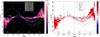 |
Fig. 2 Longitude-velocity (lv) diagrams of CO mean intensity (⟨I⟩ , left) and filament orientation anisotropy quantified by the projected Rayleigh statistic (V, right). Each pixel element in the diagrams corresponds to a 10° × 10° × 1.29 km s−1 velocity-channel map centered on b = 0°, referred to as a tile throughout this paper. Results correspond to the Hessian analysis using an 18′ FHWM derivative kernel. Values of V > 0 (red) or V < 0 (blue) indicate a preferential orientation of the filaments parallel (θ = 0°) or perpendicular (θ = 90°) to the Galactic plane. The 3σ statistical significance for these two orientations corresponds to V > 2.87 or V < −2.87, respectively. The overlaid curves correspond to the main spiral arms features presented in Reid et al. (2016), the outer Scutum-Centaurus arm (OSC, Dame & Thaddeus 2011), and the extended outer arm (M-G2004, McClure-Griffiths et al. 2004). |
4 Results
4.1 Prevalent CO filament orientation
We present the global trends for the 12CO(1–0) line emission anisotropy throughout the Galactic disk in the right-hand panel of Fig. 2. It is apparent that most of the tiles show V > 0. Notably, the highest-V tiles are clustered at positive LOS velocities in the first Galatic quadrant (QI) and at negative LOS velocities toward the fourth Galactic quadrant (QIV), corresponding to the inner Milky Way.
Figure 3 shows the distribution of V across tiles. Approximately 85% of the tiles show V > 0. Around 20% of the tiles show V > 2.87, which is the 3σ equivalent for a preferential orientation parallel to the Galactic plane. None of the tiles shows V < −2.87, and less than 0.26% show V < −1.64, indicating that a preferential orientation perpendicular to the Galactic plane is rare in the CO emission. These results hold for different initial S/N selections and other Galactic plane segmentations, with similar kernel sizes, as shown in Appendix A.
Figure 3 further confirms that most tiles with a significant preferential orientation parallel to the Galactic plane lie toward the inner Galaxy. Toward the outer Galaxy, no global anisotropy parallel or perpendicular to the Galactic plane is evident, as quantified by the predominance of |V| < 2.87 and the mean orientation angles reported in Appendix A. The latter outcome is in agreement This finding agrees with the results reported by Dib et al. (2009), who present an analysis of position angles (PAs) of MCs in the 50′′-resolution Five College Radio Astronomy Observatory (FCRAO) 12CO(1–0) survey of the Outer Galaxy (Heyer et al. 1998, 2001) and found that their orientations are random.
Figure 4 shows the variation of V with Galactocentric distance (Rgal), computed using the central vLSR of each tile and assuming circular motions around the Galactic center following the Galactic rotation model of Reid et al. (2019). Following Soler et al. (2022) and earlier works, we excluded the Galactic longitude ranges l < 15°, l > 345°, and 165° < l < 195° from the distance reconstruction. This selection aims to minimize uncertainties in Rgal caused by noncircular motions toward the Galactic center and anti-center (Hunter et al. 2024), as well as excluding the sphere of influence of the Galactic bar (Göller et al. 2025).
The scatter plot in Fig. 4 further illustrates that orientations preferentially parallel to the Galactic plane in CO emission are predominantly found at Rgal < R⊙. The asymmetry in the V distribution around Rgal = R⊙ indicates that the heliocentric distance, d, does not systematically cause lower values, due to the fixed angular size of the derivative. If the filamentary structures used to quantify anisotropy were randomized with increasing d by the spatial filtering of the derivative kernel, as illustrated with the fBm models in Appendix C, one would expect lower V at opposite sides of Rgal = R⊙ in Fig. 4, Instead, we find that the position to the Galactic center is more relevant for the level of anisotropy quantified by V.
The progressive decrease in mean V with increasing Rgal in Fig. 4 can be interpreted as a decrease in the anisotropy in the 12CO(1–0) distribution with increasing distance from the Galactic center. The prevalence of |V| < 2.87 for Rgal ≳ 9 kpc indicates mostly random orientations toward the outer Galaxy. The Galactocentric radius at which mean anisotropy levels fall below the significance threshold V = 2.87 is around 6 kpc. However, a few tiles with V > 2.87 exist at larger Rgal, up to roughly 10 kpc from the Galactic center.
Visual inspection of the l-vLSR distribution of V in Fig. 2 suggests that the high-V tiles coincide with some positions along the tracks of the Scutum-Centaurus (Sct-Cen) spiral arm toward QI and QIV. However, high-V tiles are also found outside the spiral arm tracks. The tiles along the Perseus arm (Per) show low V values, indicating a random orientation of the CO filaments for emission along the l-vLSR track.
Local structures in CO emission, defined as those at |vLSR| ≲ 20 km s−1 in Fig. 2 or Rgal ≈ R⊙ in Fig. A.1, do not show a preferential orientation. The S/N in the Dame et al. (2001) observations is insufficient to identify significant emission toward the Outer, Outer Scutum-Centaurus (OSC), and extended outer spiral arms, where the most prominent HI filaments parallel to the Galactic plane were identified by Soler et al. (2022). However, these portions of the Galactic plane have been sampled with higher sensitivity in other higher-resolution surveys, as we discuss in the following section.
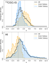 |
Fig. 3 Normalized histogram of V distribution across 10° × 10° × 1.29-km s−1 tiles for 12CO(1–0) (top), corresponding to values presented in the left-hand panel of Fig. 2, and HI, corresponding to Figure A.3 in Soler et al. (2022). The dashed vertical line marks V = 0, which corresponds to no preferential orientation either parallel or perpendicular to the Galactic plane. The dotted vertical lines indicate V = ±2.87, which correspond to the 3σ significance levels for preferential orientation parallel or perpendicular to the Galactic plane, respectively. |
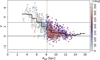 |
Fig. 4 Distribution of V as a function of Galactocentric distance (Rgal). Each marker corresponds to a 10° × 10° × 1.29 km s−1 tile on the left-hand panel of Fig. 2. Colors represent the central Galactic longitude (l) of each tile. The black solid line shows the V mean value in 1-kpcwide Rgal bins. The dashed vertical line indicates the radius of the Solar orbit, R⊙ = 8.15 kpc. The solid horizontal line marks V = 0, which corresponds to no preferential orientation either parallel or perpendicular to the Galactic plane. The dashed horizontal lines indicate V = ± 2.87, which correspond to the 3σ significance levels for preferential orientation parallel or perpendicular to the Galactic plane, respectively. |
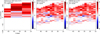 |
Fig. 5 Comparison of filament anisotropy in 10° × 10° regions from 7.′5-resolution Dame et al. (2001) 12CO(1–0) observations (left), and in 2° × 2° regions from 49′′-resolution 12CO(1–0) observations of the MWISP survey, for velocity channel widths of 1.5 km s−1 (middle) and 0.16 km s−1 (right), as reported by Soler et al. (2021). |
4.2 Comparison with higher-resolution observations
To determine the effects of the 7.′5 FWHM resolution in the Dame et al. (2001) composite survey on the results of our anisotropy analysis, we considered the portion of the Galactic plane covered by the MWISP survey 12CO(1–0) observations with roughly nine times higher angular resolution, although limited to the range |b| < 1°. The MWISP dataset was previously analyzed by Soler et al. (2021); however, we have reproduced their analysis for comparison with the global trends across the plane.
Figure 5 presents the preferential orientation throughout the 12CO MWISP observations split in 2° × 2° regions and 1.49-km s−1-wide tiles. As previously reported in Soler et al. (2021), the majority of the tiles at vLSR > 0 km s−1 show V > 2.87, suggesting that the emission is preferentially oriented parallel to the plane toward that portion of the first Galactic quadrant. Toward the outer Galaxy, vLSR < 0 km s−1, there is no predominant preferential orientation.
The agreement in the preferential filament orientations for vLSR > 0 km s−1 in the Dame et al. (2001) and MWISP observations suggests that the global anisotropy in the emission distribution remains consistent across one order of magnitude in spatial scales. Figure 6 illustrates the persistence of the global orientation of the structures in the two surveys. Although the MWISP data reveal clouds and features with different orientations in the CO emission at higher resolution, their preferential orientation maintains the global pattern identified at larger spatial scales in the Dame et al. (2001) data. The structures identified using the Hessian matrix method for the two surveys, as shown in the right panels of Fig. 6, confirm that this technique not only identifies the same large-scale structure in both surveys but also reveals small-scale structures with the same anisotropy as the coarse-resolution data.
We also compared low- and high-resolution 12CO emission data for a tile with preferentially vertical structures, identified by the lowest V in the lv-diagram on the right panel of Fig. 2. This tile, shown in Fig. 7, is covered by the FQS, which reveals that the coarse structures identified in the Dame et al. (2001) CO data resolve into smaller structures that preserve the large-scale orientation. This region exhibits filamentary structures perpendicular to the Galactic plane, rather than the prevailing alignment with the disk. This location coincides with the position of GSH 238+00+09, a nearby major superbubble toward Galactic longitude around 238° (Heiles 1998), where 12CO(1–0) emission is faint and dust extinction is singularly low (see, for example, Soler et al. 2025).
4.3 Comparison with the HI filament orientation
Figure 8 presents the comparison between the CO filament orientation trends, shown in the right panel of Fig. 2 and the equivalent analysis of filamentary structures in the HI emission, presented in the middle of Figure A.3 in Soler et al. (2022). The scatter plot shows that tiles with VCO > 2.87 tend to coincide with VHI < −2.87, indicating that the most evident anisotropy parallel to the Galactic plane in CO emission occurs where HI is preferentially perpendicular. This trend mainly corresponds to structures in the inner Galaxy.
The differing orientations of the structures traced by HI and CO emission can be potentially explained by the tile extension in Galactic latitude. The |b| < 5° covers relatively high altitudes above the disk, which are dominated by HI emission, and while a low altitudes the CO emission is more prevalent. However, the comparison of the preferential orientation in the MWISP data and the 40′′ resolution HI observations from The HI, OH, Recombination line (THOR) survey of the inner Milky (Beuther et al. 2016; Wang et al. 2020) toward the Galactic latitude band |b| < 1° indicate different preferential orientations of the two tracers at smaller scales and lower altitudes (Soler et al. 2020, 2021). This result suggests that the difference in orientations of structures traced by HI and CO emission is not exclusively due to a scale-height selection effect.
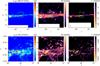 |
Fig. 6 Example of a tile with CO emission structures mostly parallel to the Galactic plane, as identified by the highest V values in the left panel of Fig. 2. The top panels show the 12CO(1–0) line emission at 7.′5 FWHM resolution in the Dame et al. (2001) composite survey. The bottom panels show the 12CO(1–0) line emission at 55′′ FWHM resolution in the MWISP survey toward the region marked with the green square in the top panel. The left, middle, and right panels show the line emission map, its gradient, and the filamentary structures identified by the second eigenvalue of the Hessian matrix (Eq. (2)) respectively. |
5 Discussion
5.1 CO orientations toward the inner and outer Galaxy
One of the main findings in our study of the anisotropy traced by the orientation of filamentary structures in 12CO(1–0) emission is the differing behavior in the inner and outer Milky Way. This is illustrated by the predominantly positive V around vLSR > 0 km s−1 toward QI and vLSR < 0 km s−1 toward QIV in the right-hand panel of Fig. 2, and by the low V for other regions and velocity ranges. It is also evident in the V trends presented in Figs. 3 and 4.
The extent of our results toward the outer Galaxy is limited by the sensitivity of the Dame et al. (2001) data. However, the higher-sensitivity and angular resolution observations from MWISP confirm the random orientations of CO structures beyond the Solar circle, as illustrated in Fig. 5. The analysis presented by Dib et al. (2009) also suggests that this may be the case for outer Galaxy CO structures in the second Galactic quadrant (QII).
The portion of the Galactic plane sampled with higher resolution and sensitivity in the MWISP survey also shows predominantly horizontal CO structures in the emission toward the inner Galaxy, as illustrated in Fig. 5. This indicates that structures parallel to the Galactic plane at 7.′5 resolution do not resolve into randomly oriented structures at 49′′ resolution. The prevalent anisotropy is similar across roughly one decade of spatial scales. This is an expected behavior given the correlations across scales introduced by turbulence in the ISM (see, for example, Elmegreen & Scalo 2004; Hennebelle & Falgarone 2012).
What we denote as the inner and outer Galaxy correspond to two domains in the CO distribution. The CO mass in the outer galaxy is between 2.3 and 2.7 times lower than in the inner Galaxy (see Heyer & Dame 2015, and references therein). The surface density profile of the CO mass also decreases by a factor of roughly five and more after Rgal ≈ 7 kpc, as illustrated in figure 7 in Heyer & Dame (2015). The CO scale height also increases from roughly a FWHM of around 100 pc for Rgal ≲ R⊙ to several times that value beyond the Solar circle, as shown in the top panel of figure 6 in Heyer & Dame (2015). The mid-plane height is also displaced by more than 100 pc for Rgal ≳ R⊙, as presented in the bottom panel of figure 6 in Heyer & Dame (2015).
The difference in the radial extent of CO can be attributed to variations in the midplane pressure, as recently shown in the numerical simulation of Smith et al. (2023). That implies that the structures traced by CO in the outer Galaxy are less constrained to remain in the plane than those within the Solar circle. Neutral atomic hydrogen (HI) observations indicate velocity dispersions between 12 and 15 km s−1 toward the central regions of nearby face-on spiral galaxies and between 4 and 6 km s−1 toward their outskirts (e.g., Ianjamasimanana et al. 2015). Turbulent velocity fluctuations associated with the observed vertical velocity field in the outer Galaxy may potentially be responsible for randomizing the orientation of CO structures in regions of lower vertical pressure.
Soler et al. (2022) identify to the energy and momentum input from clustered SNe explosions as the source of the prevalent vertical (perpendicular to the plane) HI structures toward the inner Galaxy. Toward the outer Galaxy, where the population of SN precursor high-mass stars is lower, HI filamentary structures are predominantly parallel to the Galactic plane. In the case of CO, the combination of the lower coupling of the dense gas with the input from SNe and the higher midplane pressure is the most plausible source of CO anisotropy parallel to the Galactic plane in the inner Galaxy. Toward the outer Galaxy, other sources of interstellar turbulence, such as accretion from the Galactic halo and global Galactic motions (see, for example Klessen & Hennebelle 2010; Meidt et al. 2018), can produce motions that randomize the orientation of the dense gas traced by CO with respect to the Galactic plane.
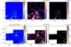 |
Fig. 7 Same as Fig. 6, but showing the tile where CO structures are mostly perpendicular to the Galactic plane, characterized by the lowest V values in the left panel of Fig. 2. The bottom panels show the 12CO(1–0) line emission at 55′′ FWHM resolution sampled in the FQS toward the region marked with the green square in the top panel. |
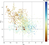 |
Fig. 8 Comparison of the preferential orientation obtained with the projected Rayleigh statistic (V, Eq. (4)) applied to 12CO(1–0) and HI observations. The latter corresponds to the results reported by Soler et al. (2020) for the same tile size and derivative kernel size. Colors indicate the Galactocentric distances of each tile. |
5.2 Relation to giant molecular filaments and other Galactic filamentary structures
The preferential orientation parallel to the Galactic plane for CO emission can also be related to the potential effect of spiral density waves (Lin & Shu 1964). Toward the inner Galaxy, where spiral density waves are presumed to be stronger due to the higher gas and stellar densities, the flows would be actively redirected along the arm. This provides a compressive component that drives preexisting small MCs to coagulate and build mass, forming larger MCs and triggering instabilities in the atomic gas that ultimately lead to further MC formation (see, for example, Roberts 1969; Pringle et al. 2001). The structures assembled through this mechanism would be long and preferentially aligned with the plane, similar to the “Nessie” filament in the Milky Way and other elongated molecular structures in nearby galaxies (see, for example, Goodman et al. 2014; Meidt et al. 2023). However, numerical studies show that a spiral potential is not essential for producing disk-aligned filamentary structures, as differential rotation elongates any density enhancement along the radial direction (see, for example, Smith et al. 2014b; Duarte-Cabral & Dobbs 2017).
Extending our analysis to identify individual structures, such as spiral arms, is complicated by the overlap of multiple structures in position-position distance (PPD) into a single velocity channel in position-position velocity (PPV) space, which is more prevalent in these regions than in the inner Galaxy. The overlap of multiple PPD structures in PPV may produce the marked anisotropy with respect to the Galactic plane observed toward the inner Galaxy. Such an anisotropy in PPV channels would not be observed if it were not initially present in the corresponding portions of the PPP volume. However, linking an individual PPP structure, such as a spiral arm, to the overall PPV anisotropy reported in Fig. 2 is not straightforward and is beyond the scope of this work.
Zucker et al. (2018) presented the physical properties of large-scale Galactic filaments identified in mid- and far-infrared emission, as well as in emission from CO and other high-density tracers. Most objects in their sample display low inclinations with respect to the Galactic plane, which agrees with our results for the general anisotropy in the CO emission.
Colombo et al. (2021) identified and characterized filamentary structures in the 12CO(2–1) emission observations in the Outer Galaxy High-Resolution Survey (OGHReS), reporting that large-scale filaments in the outer Galaxy have, on averange, masses and linear masses around one order of magnitude lower than similar structures toward the inner Galaxy. This behavior has previously been reported in comparisons of MCs in the inner and outer Galaxy and has been attributed to variations in metal-licity or dust-to-gas ratio with Rgal (see, for example, Lada & Dame 2020). Our results suggest that in addition to these effects, global physical conditions may vary with increasing distance from the Galactic center, as evidenced by different anisotropies observed in HI and CO LOS velocity channels corresponding to the inner and outer Milky Way.
5.3 Comparison with numerical simulations
A direct comparison of our analysis with synthetic observations is not yet available, primarily because galactic-scale simulations currently lack the spatial resolution to simultaneously reproduce the density structures sampled by CO and capture the large-scale dynamics. Numerical models of 1-kpc-side boxes have, however, been used to study the gas properties generated by galactic winds and fountains in a star-forming, stratified ISM. For example, Kim & Ostriker (2018) describe the differential effect of SN feedback on various gas phases, with warm and cold ISM clouds entrained by a high-velocity, low-density hot wind, which maintains the cold gas at lower scale heights than the warmer and hotter components. Stratified-box experiments by Girichidis et al. (2018b) indicate that magnetic fields increase the disk scale height and delay the formation of dense and molecular gas. Although their analysis does not explicitly address the orientation of the structures traced by CO, which are included as part of the chemical network in their model, the column density projections indicate that dense gas structures remain close to the midplane and are only momentarily parallel to the Galactic plane before SN explosions randomize their orientations.
The Galactic-scale simulations of multiphase ISM presented in Smith et al. (2020) show that spiral-arm-like structures and differential rotation preferentially align filamentary structures, whereas strong feedback randomizes their orientations. Our observations, however, indicate that most CO filamentary structures aligned with the plane are located in the inner Galaxy, where SN feedback is more concentrated. The analysis of synthetic observations of large-scale Galactic filaments presented by Zucker et al. (2019) indicates that most coherent and elongated structures have low inclinations relative to the Galactic plane.
As expected from the relatively low SFR in the Milky Way, we do not detect a prevalent signature of the Galactic outflows in the molecular gas, unlike those observed in NGC253 or M82. This absence may be due to the lack of input from direct SN feedback and the related cosmic ray (CR) pressure. Recent numerical experiments, such as those presented in Girichidis et al. (2018a), indicate that CR pressure near the midplane is comparable to other pressure components, but the scale height of CRs is much larger and can efficiently accelerate warm gas above and below the plane. More recently, Kjellgren et al. (2025) show that CRs can drive weak but sustained outflows throughout a Galactic disk simulation, suggesting that they can favor gas mixing and produce colder extraplanar gas (Fraternali & Binney 2006). This effect is not necessarily reduced to the region of CR injection, as the lifting of gas by CRs can link larger spatial scales with the fountain flows, the magnetic fields, and the resulting Parker loops that occur locally.
The differences in the orientation of structures traced by HI and 12CO(1–0) are potentially related to the distinct mass swept up and the total momentum input from SN in the gas at different densities (see, for example, Kim & Ostriker 2015; Martizzi et al. 2015). Both HI and CO experience the same large-scale gravitational potential, establishing the Galactic plane as the central axis of symmetry. However, HI is less dense and couples more efficiently to the vertical momentum input from stellar feedback, producing the chimneys observed in the vertical direction, while the densest CO clouds remain closer to the plane, as shown in the multiphase ISM numerical simulations presented in Walch et al. (2015) and Girichidis et al. (2016)1.
The CR-driven outflows have moderate launching velocities close to the midplane and are denser, smoother, and colder than the (thermal) SN-driven winds (Girichidis et al. 2016). They can drive gas at various densities, but typically act on the more diffuse gas, which means that the HI structures are more likely to be altered by CRs than those traced CO. Therefore, CRs can also help or drive the difference in the anisotropies of the structures traced by HI and CO, illustrated in Fig. 8.
5.4 Molecular gas not traced by CO
Our observations do not imply that all molecular gas follows the asymmetry indicated by the CO emission. It is likely that molecular gas is also present in the HI structures perpendicular to the Galactic plane. We cannot observe it in CO due to the low column densities, which lead to the CO destruction, whereas molecular hydrogen (H2) and dust may remain intact. Recent James Webb Space Telescope (JWST) observations of polycyclic aromatic hydrocarbon (PAH) emission reveal dust filamentary structures extending to kiloparsec-scale altitudes above the disks of edge-on galaxies NGC 891 and M82 (see, for example, Chastenet et al. 2024; Fisher et al. 2025). The presence of dust at these high altitudes challenges current understanding of the transport mechanisms involved, suggesting that small dust grains can survive for several tens of millions of years after being ejected by galactic winds at the disk-halo interface. An analysis of the relation between PAH features and CO clouds in M82 indicates that CO emission is not tracing the full budget of molecular gas in that galaxy, potentially due to photoionization and/or emission suppression of CO molecules by the hard radiation fields of the central starburst (Villanueva et al. 2025).
Identifying the molecular gas not traced by CO in the vertical structures traced by HI toward the inner Galaxy is a challenging task. Nonetheless, our study indicates that the Milky Way is unlikely to display the prominent CO chimneys seen in galaxies such as NGC253 (Krieger et al. 2019). Our results also highlight the anisotropies in the CO emission and their variation with Galactocentric radius, which are more difficult to disentangle in extragalactic systems but can provide additional information about the transport mechanisms in Galactic winds.
Our results are inevitably constrained by the limitations of CO as a molecular gas tracer. In the inner Galaxy, we may not observe the molecular gas in the ISM being lifted off the mid-plane because CO is not a reliable tracer of that gas phase. In the outer Galaxy, it is possible that CO is not tracing a more extended molecular component, as suggested by [CII] and OH emission observations of the outer Milky Way (see, for example, Pineda et al. 2013; Busch et al. 2021). Numerical studies of spiral galaxies with a time-dependent chemical network indicate that molecular gas primarily resides in long filaments that are stretched between spiral arms by galactic shear, but only the centers of these filaments are bright in CO (Smith et al. 2014a). Further observational studies of the portion of the molecular gas not traced by the CO rotational emission remain challenging. However, higher-resolution, velocity-resolved observations of HI self-absorption and OH absorption enabled by the forthcoming Square Kilometer Array (SKA) promise to reveal the distribution and physical properties of the molecular gas in a broader range of Galactic environments (Li et al. 2015; Dawson et al. 2024).
6 Conclusions
We present a study of the 12CO(1–0) line emission anisotropy across the Milky Way disk to investigate the effects of stellar feedback and galactic dynamics on the distribution of the dense interstellar gas. We find that the structures sampled with this tracer are predominantly parallel to the Galactic plane in the inner Galaxy, in clear contrast to the primarily perpendicular orientation of the structures traced by the HI 21-cm line emission toward the same regions. Our results suggest that Galactic molecular winds, traced by elongated CO structures perpendicular to the disks of starburst galaxies such as NGC891 and M82, are not currently prevalent in the Milky Way.
We also applied our analysis to portions of the Galactic plane sampled at higher resolution by other CO surveys in narrower latitude bands. We find that the structures traced by CO emission remain preferentially aligned with the Galactic plane in the inner Galaxy, but are randomly oriented beyond the Solar circle. Whether this behavior extends to other CO isotopologues or molecular tracers is beyond the scope of this work but warrants further study and may reveal important information about the coupling between scales in the Galactic ISM.
The dissimilar orientations in the HI and CO emission likely result from the variations in the midplane pressure and the effect of SN feedback on the diffuse and dense gas. In that scenario, diffuse structures traced by HI are efficiently expelled from the disk by clustered SNe. In contrast, the denser gas traced by CO tends to remain close to the midplane in regions of high pressure, such as the inner Galaxy. The midplane pressure is lower toward the outer Galaxy, as evidenced by the decreasing CO surface density. Thus, the structures traced by CO are less constrained by the disk anisotropy and exhibit random orientations, most likely because of turbulent fluctuations introduced by processes distinct from the SN feedback prevalent in the inner Galaxy.
In comparison with studies based on segmenting CO emission to define objects such as clouds and spiral arms, our analysis focuses on a general emission property to determine variations throughout the Galaxy. In addition to the variations in CO surface density, midplane height, and scale height with Galac-tocentric radius, we find that the anisotropy in the distribution of the emission in the plane of the sky also changes with increasing distance from the Galactic center. Whether this behavior corresponds to a variation in the physical mechanisms acting on the gas or a change in the CO emission distribution calls for additional studies, particularly of Galactic-scale numerical simulations. However, our results already show that the position with respect to the Galactic center influences the distribution of CO, the main molecular gas tracer, indicating a potential link between the conditions leading to star formation and the large-scale Galactic environment.
Acknowledgements
The European Research Council funds JDS via the ERC Synergy Grant “ECOGAL – Understanding our Galactic ecosystem: From the disk of the Milky Way to the formation sites of stars and planets” (project ID 855130, PIs P. Hennebelle, R. S. Klessen, S. Molinari, L. Testi). JDS also acknowledges funding from the Austrian Science Fund (Fonds zur Förderung der wissenschaftlichen Forschung, FWF) through the project “Neutral Atomic Hydrogen in the solar neighborhood” (NeAtHood; Grant DOI 10.55776/PAT6169824). Some of the crucial discussions that led to this work took place under the Milky-Way-Gaia program of the PSI2 project, which is funded by the IDEX Paris-Saclay, ANR-11-IDEX-0003-02. JDS thanks the following people for their encouragement and conversation: Fabian Walter, Henrik Beuther, Bob Benjamin, Karin Kjellgren, Lilly Kormann, and Bruce Elmegreen. RSK also acknowledges financial support from the German Excellence Strategy via the Heidelberg Cluster “STRUCTURES” (EXC 2181 – 390900948) as well as from the German Ministry for Economic Affairs and Climate Action in the project “MAINN” (funding ID 50OO2206). RSK thanks the 2024/25 Class of Radcliffe Fellows for stimulating discussions. The authors thank the anonymous referee for the comments that improved the quality of the manuscript. The computations for this work were performed at the Max-Planck Institute for Astronomy (MPIA) astro-node servers. Software: astropy (Astropy Collaboration 2018), TurbuStat (Koch et al. 2019), SciPy (Virtanen et al. 2020), magnetar (Soler 2020).
References
- Abreu-Vicente, J., Ragan, S., Kainulainen, J., et al. 2016, A&A, 590, A131 [NASA ADS] [CrossRef] [EDP Sciences] [Google Scholar]
- Astropy Collaboration (Price-Whelan, A. M., et al.) 2018, AJ, 156, 123 [Google Scholar]
- Barnes, P. J., Hernandez, A. K., O’Dougherty, S. N., Schap, W. J.III, & Muller, E. 2016, ApJ, 831, 67 [NASA ADS] [CrossRef] [Google Scholar]
- Batschelet, E. 1972, Recent Statistical Methods for Orientation Data, 262, 61 [Google Scholar]
- Batschelet, E. 1981, Circular Statistics in Biology, Mathematics in Biology (Academic Press) [Google Scholar]
- Benedettini, M., Molinari, S., Baldeschi, A., et al. 2020, A&A, 633, A147 [NASA ADS] [CrossRef] [EDP Sciences] [Google Scholar]
- Beuther, H., Bihr, S., Rugel, M., et al. 2016, A&A, 595, A32 [NASA ADS] [CrossRef] [EDP Sciences] [Google Scholar]
- Bolatto, A. D., Warren, S. R., Leroy, A. K., et al. 2013, Nature, 499, 450 [Google Scholar]
- Brunt, C. M., & Heyer, M. H. 2002, ApJ, 566, 276 [Google Scholar]
- Busch, M. P., Engelke, P. D., Allen, R. J., & Hogg, D. E. 2021, ApJ, 914, 72 [CrossRef] [Google Scholar]
- Chastenet, J., De Looze, I., Relaño, M., et al. 2024, A&A, 690, A348 [NASA ADS] [CrossRef] [EDP Sciences] [Google Scholar]
- Chung, A., Yun, M. S., Naraynan, G., Heyer, M., & Erickson, N. R. 2011, ApJ, 732, L15 [NASA ADS] [CrossRef] [Google Scholar]
- Colombo, D., König, C., Urquhart, J. S., et al. 2021, A&A, 655, L2 [NASA ADS] [CrossRef] [EDP Sciences] [Google Scholar]
- Dame, T. M., & Thaddeus, P. 2011, ApJ, 734, L24 [NASA ADS] [CrossRef] [Google Scholar]
- Dame, T. M., Hartmann, D., & Thaddeus, P. 2001, ApJ, 547, 792 [Google Scholar]
- Dawson, J. R., Breen, S. L., & Gaskap-Oh Team 2024, in IAU Symposium, 380, Cosmic Masers: Proper Motion Toward the Next-Generation Large Projects, eds. T. Hirota, H. Imai, K. Menten, & Y. Pihlström, 486 [Google Scholar]
- Dekel, A., & Silk, J. 1986, ApJ, 303, 39 [Google Scholar]
- Di Teodoro, E. M., McClure-Griffiths, N. M., Lockman, F. J., & Armillotta, L. 2020, Nature, 584, 364 [NASA ADS] [CrossRef] [Google Scholar]
- Dib, S., Walcher, C. J., Heyer, M., Audit, E., & Loinard, L. 2009, MNRAS, 398, 1201 [NASA ADS] [CrossRef] [Google Scholar]
- Duarte-Cabral, A., & Dobbs, C. L. 2017, MNRAS, 470, 4261 [NASA ADS] [CrossRef] [Google Scholar]
- Durand, D., & Greenwood, J. A. 1958, J. Geol., 66, 229 [Google Scholar]
- Elia, D., Molinari, S., Schisano, E., et al. 2022, ApJ, 941, 162 [NASA ADS] [CrossRef] [Google Scholar]
- Elia, D., Evans, N. J., Soler, J. D., et al. 2025, ApJ, 980, 216 [Google Scholar]
- Elmegreen, B. G. 2000, ApJ, 530, 277 [Google Scholar]
- Elmegreen, B. G., & Scalo, J. 2004, A&A, 42, 211 [Google Scholar]
- Fabian, A. C. 2012, A&A, 50, 455 [Google Scholar]
- Fisher, D. B., Bolatto, A. D., Chisholm, J., et al. 2025, MNRAS, 538, 3068 [Google Scholar]
- Frangi, A. F., Niessen, W. J., Vincken, K. L., & Viergever, M. A. 1998, in Medical Image Computing and Computer-Assisted Intervention – MICCAI’98, eds. W.M. Wells, A. Colchester, & S. Delp (Berlin, Heidelberg: Springer), 130 [Google Scholar]
- Fraternali, F., & Binney, J. J. 2006, MNRAS, 366, 449 [CrossRef] [Google Scholar]
- Fukui, Y., & Kawamura, A. 2010, A&A, 48, 547 [Google Scholar]
- Girichidis, P., Naab, T., Walch, S., et al. 2016, ApJ, 816, L19 [NASA ADS] [CrossRef] [Google Scholar]
- Girichidis, P., Naab, T., Hanasz, M., & Walch, S. 2018a, MNRAS, 479, 3042 [NASA ADS] [CrossRef] [Google Scholar]
- Girichidis, P., Seifried, D., Naab, T., et al. 2018b, MNRAS, 480, 3511 [NASA ADS] [CrossRef] [Google Scholar]
- Göller, J., Girichidis, P., Brucy, N., et al. 2025, A&A, in press, https://doi.org/10.1051/0004-6361/202452223 [NASA ADS] [CrossRef] [EDP Sciences] [Google Scholar]
- Goodman, A. A., Alves, J., Beaumont, C. N., et al. 2014, ApJ, 797, 53 [CrossRef] [Google Scholar]
- Hacar, A., Clark, S. E., Heitsch, F., et al. 2023, in Astronomical Society of the Pacific Conference Series, 534, Protostars and Planets VII, eds. S. Inutsuka, Y. Aikawa, T. Muto, K. Tomida, & M. Tamura, 153 [Google Scholar]
- Hayward, C. C., & Hopkins, P. F. 2017, MNRAS, 465, 1682 [Google Scholar]
- Heiles, C. 1998, ApJ, 498, 689 [NASA ADS] [CrossRef] [Google Scholar]
- Hennebelle, P., & Falgarone, E. 2012, A&A Rev., 20, 55 [Google Scholar]
- Heyer, M., & Dame, T. M. 2015, A&A, 53, 583 [Google Scholar]
- Heyer, M. H., Brunt, C., Snell, R. L., et al. 1998, ApJS, 115, 241 [NASA ADS] [CrossRef] [Google Scholar]
- Heyer, M. H., Carpenter, J. M., & Snell, R. L. 2001, ApJ, 551, 852 [NASA ADS] [CrossRef] [Google Scholar]
- Heyer, M., Di Teodoro, E., Loinard, L., et al. 2025, A&A, 695, A60 [NASA ADS] [CrossRef] [EDP Sciences] [Google Scholar]
- HI4PI Collaboration (Ben Bekhti, N., et al.) 2016, A&A, 594, A116 [NASA ADS] [CrossRef] [EDP Sciences] [Google Scholar]
- Hunter, G. H., Sormani, M. C., Beckmann, J. P., et al. 2024, A&A, 692, A216 [NASA ADS] [CrossRef] [EDP Sciences] [Google Scholar]
- Ianjamasimanana, R., de Blok, W. J. G., Walter, F., et al. 2015, AJ, 150, 47 [NASA ADS] [CrossRef] [Google Scholar]
- Jackson, J. M., Rathborne, J. M., Shah, R. Y., et al. 2006, ApJS, 163, 145 [NASA ADS] [CrossRef] [Google Scholar]
- Jaffa, S. E., Whitworth, A. P., Clarke, S. D., & Howard, A. D. P. 2018, MNRAS, 477, 1940 [NASA ADS] [CrossRef] [Google Scholar]
- Jow, D. L., Hill, R., Scott, D., et al. 2018, MNRAS, 474, 1018 [NASA ADS] [CrossRef] [Google Scholar]
- Kennicutt, R. C., & Evans, N. J. 2012, A&A, 50, 531 [Google Scholar]
- Kim, C.-G., & Ostriker, E. C. 2015, ApJ, 802, 99 [NASA ADS] [CrossRef] [Google Scholar]
- Kim, C.-G., & Ostriker, E. C. 2018, ApJ, 853, 173 [NASA ADS] [CrossRef] [Google Scholar]
- Kjellgren, K., Girichidis, P., Göller, J., et al. 2025, A&A, 700, A124 [NASA ADS] [CrossRef] [EDP Sciences] [Google Scholar]
- Klessen, R. S., & Hennebelle, P. 2010, A&A, 520, A17 [NASA ADS] [CrossRef] [Google Scholar]
- Klessen, R. S., & Glover, S. C. O. 2016, Star Formation in Galaxy Evolution: Connecting Numerical Models to Reality, Saas-Fee Advanced Course, 43 (Springer-Verlag Berlin Heidelberg), 85, 43 [Google Scholar]
- Koch, E. W., Rosolowsky, E. W., Boyden, R. D., et al. 2019, AJ, 158, 1 [NASA ADS] [CrossRef] [Google Scholar]
- Kreckel, K., Armus, L., Groves, B., et al. 2014, ApJ, 790, 26 [NASA ADS] [CrossRef] [Google Scholar]
- Krieger, N., Bolatto, A. D., Walter, F., et al. 2019, ApJ, 881, 43 [NASA ADS] [CrossRef] [Google Scholar]
- Krumholz, M. R., Bate, M. R., Arce, H. G., et al. 2014, in Protostars and Planets VI, eds. H. Beuther, R.S. Klessen, C.P. Dullemond, & T. Henning, 243 [Google Scholar]
- Krumholz, M. R., Thompson, T. A., Ostriker, E. C., & Martin, C. L. 2017, MNRAS, 471, 4061 [Google Scholar]
- Lada, C. J., & Dame, T. M. 2020, ApJ, 898, 3 [NASA ADS] [CrossRef] [Google Scholar]
- Leroy, A. K., Walter, F., Martini, P., et al. 2015, ApJ, 814, 83 [Google Scholar]
- Li, D., Xu, D., Heiles, C., Pan, Z., & Tang, N. 2015, Publ. Korean Astron. Soc., 30, 75 [Google Scholar]
- Lin, C. C., & Shu, F. H. 1964, ApJ, 140, 646 [Google Scholar]
- Mac Low, M.-M., Burkert, A., & Ibáñez-Mejía, J. C. 2017, ApJ, 847, L10 [Google Scholar]
- Mardia, K., & Jupp, P. 2009, Directional Statistics, Wiley Series in Probability and Statistics (Wiley) [Google Scholar]
- Martizzi, D., Faucher-Giguère, C.-A., & Quataert, E. 2015, MNRAS, 450, 504 [NASA ADS] [CrossRef] [Google Scholar]
- Matsushita, S., Kawabe, R., Kohno, K., et al. 2005, ApJ, 618, 712 [Google Scholar]
- McClure-Griffiths, N. M., Dickey, J. M., Gaensler, B. M., & Green, A. J. 2004, ApJ, 607, L127 [NASA ADS] [CrossRef] [Google Scholar]
- Meidt, S. E., Leroy, A. K., Rosolowsky, E., et al. 2018, ApJ, 854, 100 [NASA ADS] [CrossRef] [Google Scholar]
- Meidt, S. E., Rosolowsky, E., Sun, J., et al. 2023, ApJ, 944, L18 [CrossRef] [Google Scholar]
- Micelotta, E. R., Juvela, M., Padoan, P., et al. 2021, A&A, 647, A121 [NASA ADS] [CrossRef] [EDP Sciences] [Google Scholar]
- Miville-Deschênes, M.-A., Ysard, N., Lavabre, A., et al. 2008, A&A, 490, 1093 [NASA ADS] [CrossRef] [EDP Sciences] [Google Scholar]
- Miville-Deschênes, M.-A., Murray, N., & Lee, E. J. 2017, ApJ, 834, 57 [Google Scholar]
- Neralwar, K. R., Colombo, D., Duarte-Cabral, A., et al. 2022a, A&A, 663, A56 [NASA ADS] [CrossRef] [EDP Sciences] [Google Scholar]
- Neralwar, K. R., Colombo, D., Duarte-Cabral, A., et al. 2022b, A&A, 664, A84 [NASA ADS] [CrossRef] [EDP Sciences] [Google Scholar]
- Pereira-Santaella, M., Colina, L., García-Burillo, S., et al. 2016, A&A, 594, A81 [NASA ADS] [CrossRef] [EDP Sciences] [Google Scholar]
- Pineda, J. L., Langer, W. D., Velusamy, T., & Goldsmith, P. F. 2013, A&A, 554, A103 [CrossRef] [EDP Sciences] [Google Scholar]
- Planck Collaboration Int. XXXII. 2016, A&A, 586, A135 [Google Scholar]
- Pogosyan, D., Pichon, C., Gay, C., et al. 2009, MNRAS, 396, 635 [NASA ADS] [CrossRef] [Google Scholar]
- Pringle, J. E., Allen, R. J., & Lubow, S. H. 2001, MNRAS, 327, 663 [NASA ADS] [CrossRef] [Google Scholar]
- Ragan, S. E., Henning, T., Tackenberg, J., et al. 2014, A&A, 568, A73 [NASA ADS] [CrossRef] [EDP Sciences] [Google Scholar]
- Reid, M. J., Dame, T. M., Menten, K. M., & Brunthaler, A. 2016, ApJ, 823, 77 [Google Scholar]
- Reid, M. J., Menten, K. M., Brunthaler, A., et al. 2019, ApJ, 885, 131 [Google Scholar]
- Roberts, W. W. 1969, ApJ, 158, 123 [NASA ADS] [CrossRef] [Google Scholar]
- Saintonge, A., & Catinella, B. 2022, A&A, 60, 319 [Google Scholar]
- Sakamoto, K., Ho, P. T. P., Iono, D., et al. 2006, ApJ, 636, 685 [NASA ADS] [CrossRef] [Google Scholar]
- Salak, D., Tomiyasu, Y., Nakai, N., et al. 2018, ApJ, 856, 97 [CrossRef] [Google Scholar]
- Schinnerer, E., & Leroy, A. K. 2024, A&A, 62, 369 [Google Scholar]
- Schisano, E., Molinari, S., Elia, D., et al. 2020, MNRAS, 492, 5420 [Google Scholar]
- Schuller, F., Urquhart, J. S., Csengeri, T., et al. 2021, MNRAS, 500, 3064 [Google Scholar]
- Shan, W., Yang, J., Shi, S., et al. 2012, IEEE Trans. Terahertz Sci. Technol., 2, 593 [Google Scholar]
- Sharda, P., Ting, Y.-S., & Frankel, N. 2024, MNRAS, 532, 1 [Google Scholar]
- Smith, R. J., Glover, S. C. O., Clark, P. C., Klessen, R. S., & Springel, V. 2014a, MNRAS, 441, 1628 [NASA ADS] [CrossRef] [Google Scholar]
- Smith, R. J., Glover, S. C. O., & Klessen, R. S. 2014b, MNRAS, 445, 2900 [Google Scholar]
- Smith, R. J., Treß, R. G., Sormani, M. C., et al. 2020, MNRAS, 492, 1594 [NASA ADS] [CrossRef] [Google Scholar]
- Smith, R. J., Tress, R., Soler, J. D., et al. 2023, MNRAS, 524, 873 [Google Scholar]
- Soler, J. D. 2020, MAGNETAR: Histogram of relative orientation calculator for MHD observations [record ascl:2003.002] [Google Scholar]
- Soler, J. D., Hennebelle, P., Martin, P. G., et al. 2013, ApJ, 774, 128 [Google Scholar]
- Soler, J. D., Beuther, H., Syed, J., et al. 2020, A&A, 642, A163 [NASA ADS] [CrossRef] [EDP Sciences] [Google Scholar]
- Soler, J. D., Beuther, H., Syed, J., et al. 2021, A&A, 651, L4 [NASA ADS] [CrossRef] [EDP Sciences] [Google Scholar]
- Soler, J. D., Miville-Deschênes, M. A., Molinari, S., et al. 2022, A&A, 662, A96 [NASA ADS] [CrossRef] [EDP Sciences] [Google Scholar]
- Soler, J. D., Zari, E., Elia, D., et al. 2023, A&A, 678, A95 [NASA ADS] [CrossRef] [EDP Sciences] [Google Scholar]
- Soler, J. D., Molinari, S., Glover, S. C. O., et al. 2025, A&A, 695, A222 [NASA ADS] [CrossRef] [EDP Sciences] [Google Scholar]
- Stuber, S. K., Saito, T., Schinnerer, E., et al. 2021, A&A, 653, A172 [NASA ADS] [CrossRef] [EDP Sciences] [Google Scholar]
- Su, Y., Yang, J., Zhang, S., et al. 2019, ApJS, 240, 9 [Google Scholar]
- Sun, J. X., Lu, D. R., Yang, J., et al. 2018, Acta Astron. Sinica, 59, 3 [Google Scholar]
- Tsai, A.-L., Matsushita, S., Nakanishi, K., et al. 2009, PASJ, 61, 237 [NASA ADS] [Google Scholar]
- Umemoto, T., Minamidani, T., Kuno, N., et al. 2017, PASJ, 69, 78 [Google Scholar]
- Veilleux, S., Cecil, G., & Bland-Hawthorn, J. 2005, A&A, 43, 769 [Google Scholar]
- Villanueva, V., Bolatto, A. D., Herrera-Camus, R., et al. 2025, A&A, 695, A202 [NASA ADS] [CrossRef] [EDP Sciences] [Google Scholar]
- Virtanen, P., Gommers, R., Oliphant, T. E., et al. 2020, Nat. Methods, 17, 261 [Google Scholar]
- Walch, S., Girichidis, P., Naab, T., et al. 2015, MNRAS, 454, 238 [Google Scholar]
- Walter, F., Weiss, A., & Scoville, N. 2002, ApJ, 580, L21 [Google Scholar]
- Wang, K., Testi, L., Burkert, A., et al. 2016, ApJS, 226, 9 [NASA ADS] [CrossRef] [Google Scholar]
- Wang, Y., Beuther, H., Rugel, M. R., et al. 2020, A&A, 634, A83 [NASA ADS] [CrossRef] [EDP Sciences] [Google Scholar]
- Weiß, A., Walter, F., Neininger, N., & Klein, U. 1999, A&A, 345, L23 [NASA ADS] [Google Scholar]
- Zari, E., Frankel, N., & Rix, H.-W. 2023, A&A, 669, A10 [NASA ADS] [CrossRef] [EDP Sciences] [Google Scholar]
- Zucker, C., Battersby, C., & Goodman, A. 2018, ApJ, 864, 153 [NASA ADS] [CrossRef] [Google Scholar]
- Zucker, C., Smith, R., & Goodman, A. 2019, ApJ, 887, 186 [NASA ADS] [CrossRef] [Google Scholar]
Videos available at the SILCC website
Appendix A The Hessian analysis method
In the main body of this paper, we presented an analysis of the anisotropy traced by the filamentary structures selected using the Hessian analysis method. In this section, we illustrate the generality of our conclusions in comparison to the Hessian method input parameters and the circular statistic used to report the anisotropy results.
A.1 Data selection
We propagated the uncertainties in the 12CO(1–0) line measurements by using Monte Carlo realizations of the input data, as described in Sec. 3. An alternative error handling is obtained by applying signal-to-noise cuts to the input data. Figure A.1 shows the results of the anisotropy analysis reported on the right-hand panel of Fig. 2 without Monte Carlo realizations but with an initial cut by the signal-to-noise ratio (I/σI) in the input data. The results obtained excluding pixels with I/σI < 1.0, presented in the top panel of Fig. A.1, show a spurious signal in V for low-intensity channels. A more stringent cut of pixels with I/σI < 3.0, shown in the bottom panel of Fig. A.1, results in a clearer contrast in V between regions with signifi-cant signal and noise-dominated channels. Comparison between the bottom panel of Fig. A.1 and the right-hand panel of Fig. 2 indicates that the Monte Carlo sampling averages out some of the signals in low-12CO(1–0) emission channels. For example, for vLSR < 0 km s−1 beyond the Perseus arm and toward the third Galactic quadrant (QIII), where the 12CO(1–0) emission is faint, probably due to the expulsion of material by GSH 238+00+09.
The results reported on the right-hand panel of Fig. 2 correspond to an arbitrary segmentation of the Galactic plane employed to evaluate the anisotropy. We considered alternative segmentations, considering two separate options. First, offsetting in Galactic longitude the location of the 10° × 10° tiles employed in the main body of the paper. Second, employing 5° × 5° centered on b = 0°.
Figure A.2 presents the results obtained by adding an offset of 2.°5 to the central position of the 10° × 10° tiles used in Fig. 2. Some of the regions show different V, most likely as a result of splitting anisotropic structures in a velocity channel and combining them with less anisotropic structures in the same tile. However, the prevalence of high V toward the inner Galaxy and the random orientation of structures beyond the Solar circle is independent of the central position of the 10° × 10° tiles, as illustrated for the particular selection presented in Fig. A.2 and others tested in our analysis.
The main reason for using the 10° × 10° was the direct comparison with the results of the HI emission analysis presented in (Soler et al. 2022). However, the 7.°5 angular resolution of the Dame et al. (2001) composite survey allows for a finer segmentation. Figure A.3 presents the results obtained using a segmentation of the Galactic plane into 5° × 5° tiles centered on b = 0°. It is evident by visual comparison with the right-hand panel of Fig. 2 that the trends discussed in the main body of the paper are also present in the region |b| ≤ 5° and are persistent in the finer l segmentation.
Some features in Fig. A.3 may inspire additional interpretations. For example, the prevalence for V > 0 in a significant segment of the Perseus arm. However, this behavior is not seen in the MWISP data for the same spiral arm track in the lv-diagram, as illustrated in Fig. 5.
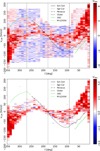 |
Fig. A.1 Same as the right-hand panel of Fig. 2, but without Monte Carlo realizations and excluding regions with signal-to-noise ratio below 1.0 (top) and 3.0 (bottom). |
A.2 Hessian method parameter selection
Two parameters are used to identify filamentary structures using the Hessian matrix. First, the derivative kernel size, which sets the spatial scale at which the filaments are singled out. Second is the critical threshold of the eigenvalue λ−, which defines the minimum curvature of the features diagnosed as filaments.
The resolution of the observations sets the minimum derivative kernel size. The analysis of the MWISP and FQS, discussed in Sec. 4, sheds light on the results obtained for smaller kernel sizes. However, the areas of the sky covered by these observations are smaller than those in the Dame et al. (2001) composite survey. We show an example of the results obtained with a larger kernel size in Fig. A.4, where we employed a 30′ FWHM derivative kernel. The amplitude of V in this example is lower, as expected from the lower number of independent gradient vectors for the same tile area. However, the main features in the V lv-diagram are coincident with those reported in the right-hand panel of Fig. 2. These results are similar for larger kernel sizes up to angular scales of roughly 1.°25, for which almost all the tiles show values below the significance level V 2.87.
We identified a critical curvature value  using the median of the values obtained in the Hessian analysis of noise-dominated velocity channels. This value may overestimate the noise level in some areas, given the sensitivity variation across the (Dame et al. 2001) composite survey. However, it provides a common denominator to filter out potential spurious filamentary structures introduced by the noise.
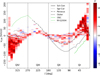 |
Fig. A.2 Same as the right-hand panel of Fig. 2, but a segmentation into 10° × 10° tiles offset by 2.°5. |
A.3 Statistics for reporting preferential orientations
On the right-hand panel of Fig. A.5, we reported the anisotropy in terms of the projected Rayleigh statistic, Eq. (4), an optimal estimator for determining the clustering of the angle data around a particular orientation (see, for example, Batschelet 1972; Mar-dia & Jupp 2009; Jow et al. 2018). In this appendix, we present the results in terms of two additional angular quantities: the Rayleigh statistic, Z, and the mean orientation angle, ⟨θ⟩, shown in Fig. A.5.
The Rayleigh statistic (or Rayleigh test; Batschelet 1972) is defined as
 (A.1)
where V correspond to the projected Rayleigh statistic defined in Eq. (4) and
(A.1)
where V correspond to the projected Rayleigh statistic defined in Eq. (4) and
 (A.2)
(A.2)
This statistic represents the general case of the projected Rayleigh statistic without setting a preferential orientation to test against. That means that high values of Z correspond to clustered data around a particular angle. Comparison between the V and Z for our anisotropy analysis, presented in Fig. A.6, shows that the high Z corresponds to high V, which is another way of showing that the filament orientation angle clustering is around 0°. This can also be confirmed by the correspondence in the distributions of V and Z presented in the right-hand panel of Fig. 2 and the top panel of Fig. A.5.
The clustering in filament orientation around 0° is also shown by the mean orientation angle, which is defined as
 (A.3)
(A.3)
The distribution of ⟨θ⟩ in the lv-diagram presented on the bottom panel of Fig. A.5 is an alternative way of visualizing our anisotropy analysis results. However, that visualization does not consider that ⟨θ⟩ can be ill-defined in tiles with a homogeneous distribution of angles or with few significant orientation measurements, as illustrated in Appendix C.
Appendix B Gradients instead of filaments as a measure of anisotropy
In the main body of the paper, we reported the results obtained using the filament orientation as a measure of anisotropy. In this appendix, we present the results of the anisotropy analysis based on the preferential orientation of intensity gradients. By definition, the gradient vectors indicate the direction perpendicular to the contours in a scalar field, such as the line emission intensity. Thus, one can quantify the anisotropy in the distribution of the structures in that scalar field by evaluating the clustering of the orientations of the gradient vectors rotated by 90°. Micelotta et al. (2021) used numerical simulations to show that the characterization of scalar fields using gradients or filaments carries complementary information about the orientation of structures. However, in our application, it is unclear a priori that the two methods for anisotropy evaluation lead to the same results.
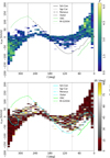 |
Fig. A.5 Same as the right-hand panel of Fig. 2, but for the Rayleigh statistic (Z) and the mean orientation angle (⟨θ⟩). |
We computed the intensity gradients in each 10° × 10° × 1.29 km s−1 channel using the same derivative kernel employed in the computation of the partial derivatives in the Hessian matrix, as described in Sec. 3. We then rotated the gradient orientation angles by 90° and used the resulting values as an input in Eq. A.1 to compute V, which we label as VGrad to distinguish it from the Hessian analysis results. Error propagation is made using Monte Carlo sampling of the noise, as in the Hessian matrix analysis.
Figure B.1 shows the anisotropy results across 12CO(1–0) line emission channels evaluated using the gradients. The distribution of VGrad is similar to the results reported in Fig. 2. The main difference is that VGrad is even closer to zero for tiles toward the outer Galaxy, highlighting the random orientation of the structures traced by 12CO(1–0) in that portion of the Milky Way.
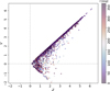 |
Fig. A.6 Relation between V and Z of the tiles presented in the right-hand panel of Fig. 2 and the top panel of Fig. A.5. The colors indicate the central Galactic longitude of each tile. |
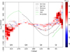 |
Fig. B.1 Same as the right-hand panel of Fig. 2, but for the 12CO(1–0) emission orientation derived from the intensity gradients. |
Appendix C Toy model tests
We evaluated the effects of beam size and structural overlap by employing fractional Brownian Motion (fBm) simulations of a 2D scalar field (Brunt & Heyer 2002; Miville-Deschênes et al. 2008). In practice, the fBm generates a random field that follows a power-law spectrum with slope –α and anisotropy defined by ellipticity ϵ and the angle θ. For this test, we chose a Kolmogorov-like spectrum, α = 3, and tested ellipticities that range between ϵ = 1.0, which corresponds to a completely isotropic scalar field, and ϵ = 0.75, 0.5, and 0.25. An example of the relationship between ϵ and the scalar field morphology is presented in Fig. C.1, where it is evident that the realizations with the same initial random but different values of ϵ display anisotropy with respect to the preferential orientation θ = 0°.
We produced 48 fBm scalar fields with 81 pixels ×81 pixels, which matches the size of the tiles analyzed in the main body of the paper. Each realization corresponds to a different initial random seed. We analyzed these fields using the Hessian method and employing different kernel sizes, expressed as multiples of the initial kernel size Ω0 = 18′. The results presented in Fig. C.2 indicate that for the same initial derivative kernel width, the anisotropy quantified with V roughly escalates linearly with ϵ. For larger kernel sizes, which can be interpreted as placing the maps at greater distances or selecting larger angular scales for filament selection, the values of V progressively decrease as the number of independent gradient vectors in each map is reduced.
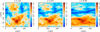 |
Fig. C.1 Synthetic emission maps produced using fBm realizations with a power spectrum slope α = 3.0, anisotropy angle θ = 0°, and ellipticities ϵ = 1.0, 0.5, and 0.25, shown from left to right. The colorbar corresponds to the amplitude of these synthetic scalar fields with mean equal to zero. |
Figure C.2 also shows the analysis of the fBm realizations in terms of ⟨θ⟩, Eq. (A.3). The large fluctuations in ⟨θ⟩ for ϵ illustrate the limitations of this metric to identify anisotropy. This is further demonstrated by the similarity of the mean values of ⟨θ⟩ for realizations with different ellipticities.
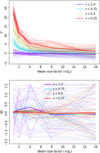 |
Fig. C.2 Anisotropy quantified by the projected Rayleigh statistic (V, top) and the mean orientation angle (⟨θ⟩, bottom) for the filamentary structures in fBm maps with ellipticities, ϵ, and for different beam sizes above the derivative kernel size Ω0 = 18′. For each color, the narrow lines correspond to the 48 fBm realizations and the broad line to the mean value of the realizations. |
All Figures
|
Fig. 1 Example of 12CO(1–0) line emission intensity (top) and the corresponding filamentary structures identified using the Hessian matrix method (bottom) toward a portion of the Galactic plane. The map shown in each color corresponds to the emission in a 1.29-km s−1-wide channel centered on the line-of-sight velocity indicated on the left-hand side of the top panel. |
| In the text | |
|
Fig. 2 Longitude-velocity (lv) diagrams of CO mean intensity (⟨I⟩ , left) and filament orientation anisotropy quantified by the projected Rayleigh statistic (V, right). Each pixel element in the diagrams corresponds to a 10° × 10° × 1.29 km s−1 velocity-channel map centered on b = 0°, referred to as a tile throughout this paper. Results correspond to the Hessian analysis using an 18′ FHWM derivative kernel. Values of V > 0 (red) or V < 0 (blue) indicate a preferential orientation of the filaments parallel (θ = 0°) or perpendicular (θ = 90°) to the Galactic plane. The 3σ statistical significance for these two orientations corresponds to V > 2.87 or V < −2.87, respectively. The overlaid curves correspond to the main spiral arms features presented in Reid et al. (2016), the outer Scutum-Centaurus arm (OSC, Dame & Thaddeus 2011), and the extended outer arm (M-G2004, McClure-Griffiths et al. 2004). |
| In the text | |
|
Fig. 3 Normalized histogram of V distribution across 10° × 10° × 1.29-km s−1 tiles for 12CO(1–0) (top), corresponding to values presented in the left-hand panel of Fig. 2, and HI, corresponding to Figure A.3 in Soler et al. (2022). The dashed vertical line marks V = 0, which corresponds to no preferential orientation either parallel or perpendicular to the Galactic plane. The dotted vertical lines indicate V = ±2.87, which correspond to the 3σ significance levels for preferential orientation parallel or perpendicular to the Galactic plane, respectively. |
| In the text | |
|
Fig. 4 Distribution of V as a function of Galactocentric distance (Rgal). Each marker corresponds to a 10° × 10° × 1.29 km s−1 tile on the left-hand panel of Fig. 2. Colors represent the central Galactic longitude (l) of each tile. The black solid line shows the V mean value in 1-kpcwide Rgal bins. The dashed vertical line indicates the radius of the Solar orbit, R⊙ = 8.15 kpc. The solid horizontal line marks V = 0, which corresponds to no preferential orientation either parallel or perpendicular to the Galactic plane. The dashed horizontal lines indicate V = ± 2.87, which correspond to the 3σ significance levels for preferential orientation parallel or perpendicular to the Galactic plane, respectively. |
| In the text | |
|
Fig. 5 Comparison of filament anisotropy in 10° × 10° regions from 7.′5-resolution Dame et al. (2001) 12CO(1–0) observations (left), and in 2° × 2° regions from 49′′-resolution 12CO(1–0) observations of the MWISP survey, for velocity channel widths of 1.5 km s−1 (middle) and 0.16 km s−1 (right), as reported by Soler et al. (2021). |
| In the text | |
|
Fig. 6 Example of a tile with CO emission structures mostly parallel to the Galactic plane, as identified by the highest V values in the left panel of Fig. 2. The top panels show the 12CO(1–0) line emission at 7.′5 FWHM resolution in the Dame et al. (2001) composite survey. The bottom panels show the 12CO(1–0) line emission at 55′′ FWHM resolution in the MWISP survey toward the region marked with the green square in the top panel. The left, middle, and right panels show the line emission map, its gradient, and the filamentary structures identified by the second eigenvalue of the Hessian matrix (Eq. (2)) respectively. |
| In the text | |
|
Fig. 7 Same as Fig. 6, but showing the tile where CO structures are mostly perpendicular to the Galactic plane, characterized by the lowest V values in the left panel of Fig. 2. The bottom panels show the 12CO(1–0) line emission at 55′′ FWHM resolution sampled in the FQS toward the region marked with the green square in the top panel. |
| In the text | |
|
Fig. 8 Comparison of the preferential orientation obtained with the projected Rayleigh statistic (V, Eq. (4)) applied to 12CO(1–0) and HI observations. The latter corresponds to the results reported by Soler et al. (2020) for the same tile size and derivative kernel size. Colors indicate the Galactocentric distances of each tile. |
| In the text | |
|
Fig. A.1 Same as the right-hand panel of Fig. 2, but without Monte Carlo realizations and excluding regions with signal-to-noise ratio below 1.0 (top) and 3.0 (bottom). |
| In the text | |
|
Fig. A.2 Same as the right-hand panel of Fig. 2, but a segmentation into 10° × 10° tiles offset by 2.°5. |
| In the text | |
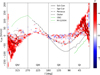 |
Fig. A.3 Same as the right-hand panel of Fig. 2, but 5° × 5° tiles centered on b = 0°. |
| In the text | |
 |
Fig. A.4 Same as the right-hand panel of Fig. 2, but 30′ FWHM derivative kernel. |
| In the text | |
|
Fig. A.5 Same as the right-hand panel of Fig. 2, but for the Rayleigh statistic (Z) and the mean orientation angle (⟨θ⟩). |
| In the text | |
|
Fig. A.6 Relation between V and Z of the tiles presented in the right-hand panel of Fig. 2 and the top panel of Fig. A.5. The colors indicate the central Galactic longitude of each tile. |
| In the text | |
|
Fig. B.1 Same as the right-hand panel of Fig. 2, but for the 12CO(1–0) emission orientation derived from the intensity gradients. |
| In the text | |
|
Fig. C.1 Synthetic emission maps produced using fBm realizations with a power spectrum slope α = 3.0, anisotropy angle θ = 0°, and ellipticities ϵ = 1.0, 0.5, and 0.25, shown from left to right. The colorbar corresponds to the amplitude of these synthetic scalar fields with mean equal to zero. |
| In the text | |
|
Fig. C.2 Anisotropy quantified by the projected Rayleigh statistic (V, top) and the mean orientation angle (⟨θ⟩, bottom) for the filamentary structures in fBm maps with ellipticities, ϵ, and for different beam sizes above the derivative kernel size Ω0 = 18′. For each color, the narrow lines correspond to the 48 fBm realizations and the broad line to the mean value of the realizations. |
| In the text | |
Current usage metrics show cumulative count of Article Views (full-text article views including HTML views, PDF and ePub downloads, according to the available data) and Abstracts Views on Vision4Press platform.
Data correspond to usage on the plateform after 2015. The current usage metrics is available 48-96 hours after online publication and is updated daily on week days.
Initial download of the metrics may take a while.