| Issue |
A&A
Volume 704, December 2025
|
|
|---|---|---|
| Article Number | A64 | |
| Number of page(s) | 13 | |
| Section | Interstellar and circumstellar matter | |
| DOI | https://doi.org/10.1051/0004-6361/202555118 | |
| Published online | 08 December 2025 | |
From theory to observation: Understanding filamentary flows in high-mass star-forming clusters
1
Max Planck Institute for Astronomy,
Königstuhl 17,
69117
Heidelberg,
Germany
2
Fakultät für Physik und Astronomie, Universität Heidelberg,
Im Neuenheimer Feld 226,
69120
Heidelberg,
Germany
3
Department of Physics and Astronomy, McMaster University,
Hamilton,
ON
L8S 4M1,
Canada
4
Origins Institute, McMaster University,
Hamilton,
ON
L8S 4M1,
Canada
5
Center for Astrophysics, Harvard & Smithsonian,
60 Garden Street,
Cambridge,
MA
02138-1516,
USA
6
National Radio Astronomy Observatory,
800 Bradbury SE, Suite 235,
Albuquerque,
NM
87106,
USA
★ Corresponding author: This email address is being protected from spambots. You need JavaScript enabled to view it.
Received:
11
April
2025
Accepted:
6
October
2025
Abstract
Context. Filamentary structures on parsec scales play a critical role in feeding star-forming regions, where they often act as the main channels through which gas flows into dense clumps that foster star formation. It is crucial to understand the dynamics of these filaments to explain the mechanisms of star formation in a range of environments.
Aims. We used data from multi-scale galactic magnetohydrodynamics simulations to observe filaments and star-forming clumps on dozens of parsec scales and investigate flow rate relations along and onto filaments as well as flows towards the clumps.
Methods. Using the FilFinderPPV identification technique, we identified the prominent filamentary structures in each data cube. Each filament and its corresponding clump were analysed by calculating the flow rates along each filament towards the clump, onto each filament from increasing distances, and radially around each clump. This analysis was conducted for two cubes, one feedback-dominated region, and one cube with less feedback, as well as for five different inclinations (0, 20, 45, 70, and 90 degrees) of one filament and clump system.
Results. The face-on inclination of the simulations (0 degrees) shows different trends depending on the environmental conditions (more or less feedback). The median flow rate in the region with more feedback is 8.9 × 10⁻⁵ M⊙yr−1, and the flow rates along the filaments towards the clumps generally decrease in these regions. In the region with less feedback, the median flow rate is 2.9 × 10⁻⁴ M⊙yr−1 and along the filaments, the values either increase or remain constant. The order of magnitude of the flow rates from the environments onto the primary filaments suffices to sustain the flow rates along these filaments. The effects of galactic and filamentary inclination also show that when the filaments are viewed from different galactic inclinations, feeder structures become clear (smaller filamentary structures that aid in the flow of material). Additionally, considering the inclination of the filaments themselves allowed us to determine by how much we over- or underestimated the flow rates for these filaments.
Conclusions. The different trends in the relation between flow rate and distance along the filaments in the feedback and non-feedback dominated cubes confirm that the environment is a significant factor in accretion flows and their relation with the filament parameters. The method we used to estimate these flow rates, which was previously applied to observational data, produced results that are consistent with those obtained from the simulations themselves. We are therefore very confident in the flow-rate calculation method.
Key words: methods: numerical / methods: observational / stars: formation / stars: massive / ISM: kinematics and dynamics / ISM: structure
© The Authors 2025
 Open Access article, published by EDP Sciences, under the terms of the Creative Commons Attribution License (https://creativecommons.org/licenses/by/4.0), which permits unrestricted use, distribution, and reproduction in any medium, provided the original work is properly cited.
This article is published in open access under the Subscribe to Open model.
Open Access funding provided by Max Planck Society.
1 Introduction
Giant molecular clouds (GMCs) serve as essential structures within galaxies, where they act as intermediaries (on the order of several tens of parsecs) that connect large-scale galactic dynamics to the smaller-scale localised star formation processes. The collapse and fragmentation of GMCs into dense regions capable of star formation is driven by a combination of gravitational instabilities and external pressures from the surrounding interstellar medium (e.g. Zinnecker 1984; Bonnell et al. 2003; André et al. 2014; Urquhart et al. 2018; Svoboda et al. 2019; Padoan et al. 2020 ). As these clouds cool and accumulate mass, they fragment into smaller denser regions under gravitational contraction. With extreme temperatures and pressures, these smaller dense regions continue to collapse and form clusters of protostellar objects. The intersections within these filamentary networks, known as hubs, often serve as sites for the formation of high-mass stellar clusters, where the convergence of gas flows provides perfect conditions for the majority of stellar births (e.g. Lada & Lada 2003; Goldsmith et al. 2008; Myers 2009; André et al. 2010; Schneider et al. 2010; Bressert et al. 2010; Kirk et al. 2013; Krumholz 2014; Kumar et al. 2020; Grudić et al. 2021; Hacar et al. 2025). The scales here are also self-similar: GMCs are hub sites on larger scales as well (e.g. Zhou et al. 2024. These filaments and filament-like structures have been a part of the discussion for years in different shapes and forms. They were studied in different tracers and as a part of many different studies theoretically and observationally, such as Fiege & Pudritz 2000; Jackson et al. 2010; Kirk et al. 2013; Gómez & Vázquez-Semadeni 2014; Henshaw et al. 2014; Chira et al. 2018; Padoan et al. 2020; Alves et al. 2020; Beuther et al. 2020; Schisano et al. 2020; Hacar et al. 2023; Pillsworth & Pudritz 2024; Wells et al. 2024). Evidence for the feeding of clouds, clumps, and cores by filamentary structures was reported in many of these studies. These studies highlighted that filaments that range in scale from galactic kiloparsec scales down to sub-parsec levels connecting the parental molecular clouds, cluster-forming hubs, clumps, and individual cores. They demonstrated the critical role the filaments play in channelling mass and angular momentum. Despite the progress made in understanding filamentary structures and their role in star formation, several questions remain. The precise mechanisms by which material is transported through, along, and around filamentary networks are still not well defined, and their impact on the formation of high-mass star clusters is still not completely understood. Current simulations and observations continue to challenge our understanding of these processes, which emphasises the need for further research to unravel the complexities of filament dynamics and their contributions to stellar cluster formation.
The advancement of theoretical model capabilities combined with large millimetre and sub-millimetre interferometers, such as the Atacama Large Millimeter and submillimeter Array (ALMA), the Northern Extended Millimeter Array (NOEMA), and the Submillimeter Array (SMA), has allowed in-depth research into more complex galactic structures such as filaments on multiple scales. Observational (e.g. Ragan et al. 2014; Zucker et al. 2015; Russell et al. 2017; Hacar et al. 2018; Olivares et al. 2019) and computational (e.g. Gómez & Vázquez-Semadeni 2014; Federrath et al. 2016; Haid et al. 2019; Li & Klein 2019; Padoan et al. 2020; Zhao et al. 2024) studies complement each other by using observational constraints in models or theoretical limitations in an observational analysis. This allows the field to progress further (e.g. Clark et al. 2014; Hillel & Soker 2020; Duan & Guo 2024). This collaborative approach is often underscored in reviews of the field, such as those by André et al. 2014; Pineda et al. 2023, who emphasised the importance of combining theoretical and observational perspectives. Together, these methods advance our understanding of the nature of filaments and allow researchers to investigate their dynamics and trace their evolution in unprecedented detail.
We used data cubes from the simulations by Zhao et al. (2024). For our observational approach, we used position-position-velocity (PPV) data drawn from these simulations chosen at five different inclination angles (0, 20, 45, 70, and 90 degrees, assuming that face-on is 0) and for two different environments (more and less feedback). We measured the flow rate properties along filaments, onto filaments, and radially onto cluster-forming clumps. We investigated larger-scale relations between the flow rates and the filamentary parameters, the environment, and the inclination. A major feature of this work is that we also tested the validity of observational methods by comparing the calculated values from our observational method with those from the full numerical position-position-position (PPP) data from the simulation. This information is not available from observations of real systems.
The structure of the paper is as follows: we introduce the simulation data in Sect. 2. In Sect. 3.1, we introduce FilFinder, the package we used to identify filaments in the PPV data cubes, and we discuss the different parameters. We present the details of the calculation of the perpendicular, parallel, and polar flow rates in these regions in Sect. 3, before we show the results of the observational method in Sect. 4. The results of the analysis of the flow rates deduced from the 3D simulation PPP data and their comparison to the observational method are then presented in Sect. 5. Finally, we discuss in Sect. 6 the results, including other scales and comparisons with observations from several programs, before we draw our conclusions and discuss opportunities for future work in Sect. 7.
2 Simulation data
We used data from multi-scale MHD simulations of a Milky Way-type galaxy from Zhao et al. (2024). These simulations were run in RAMSES with the AGORA project initial conditions (Kim et al. 2016). They include a dark matter halo with MDM halo = 1.074 × 10¹² M⊙, RDM halo = 205.5 kpc and a circular velocity of vc,DM halo = 150 kms−1, an exponential disc with Mdisc = 4.297 × 10¹⁰ M⊙, and a stellar bulge with Mbulge = 4.297 × 10¹⁰ M⊙ (Kim et al. 2016; for further simulation details, we refer to Zhao et al. 2024; Kim et al. 2016).
Recently, Pillsworth et al. (2025) characterised the properties of over 500 galactic scale filaments in the Zhao et al. (2024) simulations using the Filfinder package (Koch & Rosolowsky 2015). The authors derived the mass distribution function and gravitational stability of filaments, but did not investigate their flow dynamics.
We specifically focus on the so-called active and quiet zoom-in regions within the galactic disc of Zhao et al. (2024). Figure 1 shows this galaxy in the central panels. The two regions we used are shown at the top, and the zoom-in panels are shown at either side. The active region (right panels) is dominated by feedback in an area of converging superbubbles, and the quiet region (left panels) has less feedback and is in a spiral arm-like area of the galaxy. These zoom-in regions are 3 kpc wide boxes around dense protoclusters that achieve a spatial resolution of up to 0.28 pc. We extracted data from 60 pc around the densest cell to focus on the star-forming cluster.
In Fig. 2, we show the two regions in projected density. These figures outline the larger-scale gas flows. Panel (a) shows the feedback-dominated region in which the gas flows onto the filamentary structures. This is caused by the feedback of the surrounding superbubbles. The velocities there have ordered gradients with clearly increasing trends. The direction points towards the central clump. Panel (b) shows the non-feedback region, where the velocities on larger scales are almost parallel to the dense filament, whereas on small scales, the velocity field appears to be more chaotic and leads to the many clumps. The magnetic field lines displayed in white show that they are more disordered in the region with less feedback (panel (b)), where as in panel (a), which has more feedback, the lines follow the filament structure in parallel.
The extracted cubes were run through a position-position-velocity (PPV) post-processing code using YT (Turk et al. 2011) and the YT astro-analysis extension1. This step is key for the observational comparison because observations only produce PPV data cubes and not position-position-position (PPP) data cubes. The cubes have 212 × 212 pixels at a resolution of 1 px = 0.285 pc with velocity channels at a resolution of 0.8 kms−1. This is similar to resolutions in observation data (Wells et al. (2024)). Spatially, this is similar to larger-scale single-dish data. The galactic rotation was corrected for at a later point in the analysis, and the bounds of the velocity channels therefore change with inclination as the rotation of the galaxy becomes more dominant. The velocity range of the face-on (0 degrees) cubes is −19.6 kms−1 to 19.6 kms−1. The PPV processing does not include any spectral line post-processing on the data, and it instead returns column densities of the areas in cm−2.
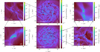 |
Fig. 1 Galaxy overview from Zhao et al. (2024). The central panels show the two snapshots of the galaxy we used, the top panel shows the location of the region with less feedback (quiet), and the bottom panel shows the location of the feedback-dominated region (active). The first zoom-in panels show the regions down to a few kiloparsec (top left and bottom right panels), followed by the close-ups of the regions in 100 × 100 pc boxes (bottom left and top right panels). |
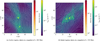 |
Fig. 2 Density projections of high-resolution zoom-in simulation data of Zhao et al. (2024). The white streamlines represent the magnetic field structure. The arrows show velocity direction and magnitude relative to the velocity of the central cores in each snapshot. |
3 Methods
To estimate the flow rates associated with the identified filamentary structures in each of the regions, we followed the approach outlined by Wells et al. (2024), which was based on Beuther et al. (2020). The mass-flow rates M˙ were estimated as
 (1)
where Σ is the surface density in units of g cm−2, directly taken from the data cube, ∆v is the velocity difference in kms−1, calculated in different ways depending on whether it is along, onto, or polar (see Sect. 3.2). w is the width of the area along which the flow rate is measured in AU. We used two pixels (0.58 pc). The final values of M˙ were converted into M⊙yr−1. The correction factor of tan(i)−1 is for the unknown filament inclination, based on the discussion by Wells et al. (2024). We did not apply this correction directly, but we investigate the inclination separately in Sect. 4.3.1.
(1)
where Σ is the surface density in units of g cm−2, directly taken from the data cube, ∆v is the velocity difference in kms−1, calculated in different ways depending on whether it is along, onto, or polar (see Sect. 3.2). w is the width of the area along which the flow rate is measured in AU. We used two pixels (0.58 pc). The final values of M˙ were converted into M⊙yr−1. The correction factor of tan(i)−1 is for the unknown filament inclination, based on the discussion by Wells et al. (2024). We did not apply this correction directly, but we investigate the inclination separately in Sect. 4.3.1.
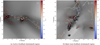 |
Fig. 3 Zeroth-moment maps of the column density cubes with the identified filamentary structure, colour-coded by velocity, are overlaid. The 2.85 pc scale bars are shown in the top right corners. |
3.1 Filament identification
We identified filaments in the PPV cubes using FilFinder (Koch & Rosolowsky 2015). Specifically, we used the FilFinder new 3D identification technique (to be presented in Koch et al., in prep.), which was also used to identify 3D filaments by Zucker et al. (2021) and Mullens et al. (2024). FilFinder in 3D uses similar morphological operations to the previous 2D version, namely adaptive thresholding, to identify locally bright structure over a wide dynamic range. One key change is the use of FilFinder of the skan package to improve the efficiency in handling 3D skeleton structures (Nunez-Iglesias et al. 2018).
We used the following steps and parameters to define the filaments we investigated in the subsequent analyses. First, we created a binary filament mask using a local threshold (adapt_thresh) and only kept structures above a minimum surface density (glob_thresh) with a minimum number of contiguous pixels (min_size) to minimise spurious isolated peaks. The resulting mask was skeletonised to produce the filament spines and structure for further analysis and pruning of spurious branches on the skeleton. Table 1 shows our choice of these key parameters for the different cubes we analysed. Lastly, we note that FilFinder is optimised to work on elongated filamentary structures with aspect ratios of 3:1. The masking and pruning operations described above naturally remove compact and isolated structures, but we note that isolated compact structures without surrounding filamentary structures were not found in the simulated cubes we analysed. For our analysis, we defined the location of the filament and its extent using the pruned skeletons produced by FilFinder.
3.2 Velocity difference
For this analysis, we investigated three different types of flow fields and rates: the flow of material along filamentary structures towards the central cluster-forming clumps; the flow of material from the environment onto the filamentary structures; and the radial inflow around the cluster (designated polar) towards the forming clumps. Each of these flow fields needs a slightly different method for calculating the velocity difference, and these methods are outlined in the following sections.
The flow-rate equation we used in this analysis works on assumptions regarding the cause of the velocity differences. Rotational signatures cannot be ruled out, but when we looked along the filament, we minimised effects from the rotation of the filament. Towards the central clumps, where local rotation or shear may occur, previous studies (e.g. Xu et al. 2020, 2024) showed that these motions contribute minimally.
FilFinderPPV parameters.
3.2.1 Along
We calculated the velocity gradient along the filament between each point on the filament spine and the hub, where the filaments converge. These hubs are typically cluster-forming regions, and we refer to them as clumps throughout this work. In Fig. 4, the green points indicate the positions along the filament at which we calculated the flow rates. We used between 30–50 points per filament at distance increments of 0.58 pc (2 px). We used the velocity value identified by FilFinder along the filament and calculated the difference between this value and the clump velocity, which was estimated by fitting a Gaussian to the spectrum at the central pixel of the clump.
3.2.2 Onto
To calculate the flow rate onto the filaments, we took four positions on either side of the filament (red points in Fig. 4) at distance increments of 0.58 pc (2 px). The velocity difference was calculated in reference to the point at which the perpendicular points meet the filament. For the perpendicular points, we used the Gaussian fit to the spectrum method to derive the velocity at the point, and the velocity on the filament was the same as above.
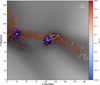 |
Fig. 4 Zeroth-moment map of the active column density cube with the identified filamentary structure, colour-coded by velocity, is overlaid. The green, red, and blue points indicate the different types of the flow rate. Green is along the filamentary structure, red is onto, and blue is polar around the clumps. The 2.85 pc scale bar is shown in the top right corner. |
3.2.3 Polar
Clumps are fed by a number of filaments. We calculated the flow rates radially outwards from the core along these converging filaments to include the contributions from each of the primary and feeder filaments (filamentary sub-structures), and the contributions from the environment surrounding the clump in the absence of any filamentary structures. We define feeder filaments as smaller filamentary structures that aid in the flow of material either onto the primary filaments or onto the central star-forming clump. These positions are marked by the blue points in Fig. 4, again at distance increments of 0.58 pc. At these points we take a Gaussian fit to the velocity spectrum for their velocity values, and the difference was considered in relation to the core velocity, which we also calculated with this method.
3.3 Error analysis
Our flow rate equation consists of three parameters. Two parameters were taken directly from the data cube itself, that is, the column density and the spatial resolution. The velocity values (identified by FilFinder or by a Gaussian fit) introduce the majority of the error to the final flow-rate values. The velocity resolution in the cubes was 0.8 kms−1, and we therefore took an estimate for the FilFinder skeleton identification error to be one channel, 0.8 kms−1. We took between 10 and 20% as the average error of the Gaussian fit. We ∼conservatively assumed an uncertainty of 20% on the estimated flow rates. We note that the uncertainties in real observations are larger because systematic errors from the column density estimates and projection effects are added. These values are without error bars in our analysis because they were taken directly from the simulations.
4 Results: Observational method
In this section the flow rates calculated with the observational method, detailed in Sect. 3, are presented. The flow rates taken directly from the 3D numerical data are shown in Sect. 5, where we also compare them with those deduced by the observational method. We broaden the scope of our results by comparing them with measurements from other observational programs in Sect. 6.
We calculated the flow rates along and onto the filaments for the active and quiet regions at 0 deg inclination and produced the histograms shown in Figs. 5 and 6. The distribution in the left panel of each figure shows flow rates along the filaments, and the distribution on the right corresponds to flow rates onto the filaments.
In Fig. 5, we present flow rate distributions for flow rates along the filaments (left panel) and onto the filaments (right panel) in the active cube. These range between 10−8 M⊙yr−1 and 10−2 M⊙yr−1 with median values of 8.9 × 10⁻⁵ M⊙yr−1 along and 2 × 10⁻⁵ M⊙yr−1 onto. The mean and median values of the active distributions are also similar within our reported errors (see Sect. 3.3). Fig. 6 shows the same, but for the quiet cube. Here, the range of flow rates is between 10−7 M⊙yr−1 and 10−1 M⊙yr−1, with median values of 2.9 × 10⁻⁴ M⊙yr−1 along and 2.3 × 10⁻⁵ M⊙yr−1 onto. This figure also shows that the quiet region differs significantly between the distribution for along and onto the filaments. Their medians are separated by a whole order of magnitude.
The distribution for the flow rates onto the filaments is wider for the active and quiet cubes. These values range from being right next to the filament to ∼2.5 pc away, so there is likely to be a large variation. We would like to note that the flow rates onto the filaments were estimated only at selected cuts across them, but that ultimately, gas flows onto the filament everywhere. Therefore, the flow rates onto the filaments have to be considered as lower limits. Based on the difference of only an order of magnitude in these individual cuts, we conclude that the flows onto are more than enough to be feeding the flows along the filament and towards the central clumps.
4.1 Along
For flows along the filaments, we analysed four different filaments in each region and focused on flows directed towards the clumps. In the active region (Fig. 7), the flow rates of the filaments increase with distance from the clump. This is consistent with the idea that the material at large scales feeds whole clusters and that this feeding closer to the central clumps can split into several separate flows, which was also reported on smaller scales (e.g. Padoan et al. 2020).
The quiet region (Fig. 8) shows different trends, however. In two instances, the flow rates decrease with the distance to the clump (top two panels in Fig. 8), and the relation after initial peaks is also more costant (potentially due to the higher column density). The comparison of the filament morphology in both regions reveals that these differences can be explained by the presence and distinct roles of feeder filaments alongside the main filaments we analysed. In the active region, feeder filaments primarily occur at the clump end of the main filaments. Here, the main filament splits into feeders as it approaches the hub, channelling the high flow rates across multiple paths and thereby reducing the flow rates closer to the core on the main filament. In contrast, the quiet region shows a different pattern. Feeder filaments are not concentrated near the hub, but are distributed along the length of the main filaments. These feeders merge into the main filaments at various points, which results in higher flow rates that reach the central hubs.
This concept also accounts for the velocity peaks in the top panels of Fig. 8, which correspond to the locations in which these feeders join the main filaments. In the bottom panels of Fig. 8, the trends begin with high flow rates close to the clump before they even out to constant flow rates with distance. This initial peak can be attributed to the column density contributions from the extended area around the core, where the column densities are higher.
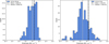 |
Fig. 5 Distributions of the flow rates. Left: along filaments. Right: onto the filaments in the active cube. |
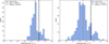 |
Fig. 6 Distributions of the flow rates. Left: along filaments. Right: onto the filaments in the quiet cube. |
4.2 Polar
By examining the flow rates radially around the central star-forming clumps, we identified the directions from which the largest contributions of material to the hub clump arise. Figures 9 and 10 show the flow-rate values around each clump in both cubes. The overlaid red and blue lines show where the main filaments connect to the hub and where the feeder filaments are. There are far more feeder filaments around clumps in the active cube, and their contribution is significant to the flow of material onto the clump. The quiet cube, in contrast, has almost no contributions outside of its main filaments that connect to the clumps. Figs. 9 and 10 show that from most angles around the clumps, there is a gradient where the flow rate increases towards the centre. This agrees with what we show in Figs. 7 and 8. At many angles around each clump at small scales (∼1 pc) in the active and quiet regions, significant contribution to the flows onto the clump from the environment is visible as well, without the use of filamentary structures.
4.3 Inclination
Another important aspect of this work was the ability to investigate inclination effects on the flow rates. We study the filamentary and galactic inclination in the following sections.
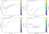 |
Fig. 7 Distance vs. flow rate in log space and relation for each filament in the active cube (filaments are labelled in Fig. 3a), colour-coded by velocity difference. |
4.3.1 Galactic
The inclination angle of the filament and galactic disc directly influences the magnitude of the velocities that are measured in observations. Although the inclination angle of the galactic disc can typically be measured in external galaxies, the inclination effects of filaments in the Milky Way are often poorly constrained. This uncertainty motivated us to study the effects of galactic and filament inclination on our estimated measurements of the flow rates along the filamentary structures towards the central clump in detail.
To pursue this goal, we studied one filament and clump structure from the active region on which we focused throughout inclinations of 0 (face on), 20, 45, 70, and 90 (edge on) degrees. The results are shown in Fig. 12. Throughout the five inclinations, the relation between distance and flow rate varies by a factor of 10. Initial peaks lie at 0 and 20 degrees, and then the rate drops slightly, before the distance and flow rate steadily increase by an order of magnitude for 0 degrees to ∼10−3.5 M⊙yr−1 and for 20 degrees to ∼10−2.5 M⊙yr−1. At 45 degrees, the values are almost constant around 10−3 M⊙yr−1. At the final two inclinations of 70 and 90 degrees, the values start lower, at 10−4 M⊙yr−1, than the previous inclinations before they increase. They peak around 10−2.5 M⊙yr−1 and plateau to become constant at larger distances from the clump, around 10−3 M⊙yr−1. We also calculated the flow rates onto the filament at each inclination. The median values for each inclination are all about 10−5 M⊙yr−1 and range between 1–7 × 10⁻⁵ M⊙yr−1, with a small increasing trend from 0 to 90 degree inclination.
4.3.2 Filament
The filament inclination with respect to the galactic plane is more complicated. The filament is in the plane of the sky when there is no velocity gradient, but otherwise, the inclination angle is often treated as unknown in observational studies. For example, Wells et al. (2024) estimated the effects of unknown inclination values on the final flow values. They reported that with an unknown inclination angle, the spread in the flow-rate values is broader and that the distribution peaked close to the true flow rate. Based on simulation data, we obtained an estimate for an average inclination along the filament with respect to the galactic plane. We measured the angles of the filaments with respect to the galactic plane by sampling direction vectors along the 3D spines of the filaments. The angle between the two vectors is easily determined via their dot product. We measured the circular mean both unweighted and weighted by the parallel flow rate to calculate the average inclination for the entire filament. We calculated the weighted mean using the parallel flow rate at each point along the spine as the weight. The regions closer to the forming cluster with higher flow rates are therefore weighted more heavily by the value of the inclination.
The results presented in Sect. 4.3.1 show the effects of galactic inclination where we incrementally increased the galactic inclination from 0 degrees (face-on) to 90 degrees (edge-on). The range of velocity differences increases in the inclined cubes relative to the face-on cube. As a result, trends appear at all inclinations shown in Fig. 12 with typical flow rates of 10−3 M⊙yr−1 to 10−4 M⊙yr−1. The inclination and the feeder filaments work together in this region to create different effects. The unknown inclination here has similar effects on the feeder filaments as the primary filament. On the other hand, the galactic inclination rotates the filament, with the potential to reveal other feeder filaments or more details about the structures that are not apparent from other angles.
In Figure 11, we present 3D plots of the filaments we identified. Importantly, these show the position relative to the midplane of the galactic disc (shown by the light purple plane in the plot). This cluster-forming area sits 313 pc above the mid-plane of the galaxy, just within one scale height of the galaxy. For filament 1, we measured an unweighted average of |49.8|◦ and a flow-rate-weighted average of |48.4|◦. The two averages are consistent within the error, which implies that the angle is similar along the entire filament. For filament 3, we measured an unweighted average angle of |10.9|◦ and a flow-rate-weighted average of |0.8|◦. From this, we deduce that the angle with respect to the plane is varies along the entire filament, with the highest flow-rate areas closest to the clump tending to be more parallel to the plane. We note that neither of these filaments is coplanar with the galaxy midplane because they sit more than 300 pc above the midplane, as shown in Figure 11.
Taking the flow-rate-weighted average inclination angles we estimated from the simulation into account, we compared the affect of the 1/tan(i) inclination correction factor on the distribution of the flow rates for these two filaments. For filament 1, we found 1/tan(i) ∼ 0.8, which means that our observed flow rates for this filament are slightly overestimated when the inclination angle is unknown. For filament 3, however, the inclination factor is 1/tan(i) ∼ 72, meaning that our estimates are underestimated by over an order of magnitude. This is clear in the bottom panel of Fig. 7, where filament 3 has the lowest flow rates of the region. In general, it is important to consider the unknown inclination angles when measuring and discussing observational flow rates because they are a key factor in accurately interpreting the results and understanding the flow behaviour.
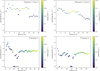 |
Fig. 8 Distance vs flow rate in log space, and relation for each filament in the quiet cube (filaments are labelled in Fig. 3a), colour-coded by the velocity difference. |
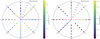 |
Fig. 9 Relation of radial distance to the flow rate for eight different angles around each clump in the active region. Numbers from 0.5 to 3.5 represent the distance from the centre for each of the concentric circles in pc. The dashed red lines indicate the primary filaments, and the solid blue lines indicate the directions of the feeder filaments. |
 |
Fig. 10 Relation of the radial distance to the flow rate for eight different angles around each clump in the quiet region. Numbers from 0.5 to 3.5 represent the distance from the centre for each of the concentric circles in pc. The dashed red lines indicate the primary filaments, and the solid blue lines indicate the directions of the feeder filaments. |
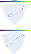 |
Fig. 11 3D projection of the filament spines for filaments 1 (top) and 3 (bottom) in the active cube. The colour bar shows the parallel flow rate at that point in the spine, and the grey markers depict the points for which the direction vector of the spine was null. The light purple plane surface shows the position of the galaxy midplane. An interactive version of this figure is available in the online version of this paper. |
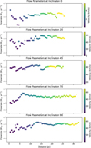 |
Fig. 12 Effect of the galactic inclination on the relation of distance vs. flow rate in log space for filament 1 from the active region. The results are shown for five different galactic inclinations of 0, 20, 45, 70, and 90 degrees. |
5 3D simulation flow rates and comparison with the observational method
A particularly interesting aspect of these observed measured flow rates for each filament is that we can directly compare them to their true values from the full 3D simulation data. In this section, we provide these true values by taking an approximation of the filament in 3D. This is achieved by masking the (x, y) values contained in the skeleton and determining the peak density along the z-axis at each point. Within the region we explored, the maximum density in z represents the third dimension of the spine of the filament, assuming the spine is aligned with the dense ridge of the filament (as is done in filament profile fitters, e.g. RadFil in Zucker & Chen 2018). We visually confirmed the connectivity of this filament by ensuring that the z-values contribute to a continuous filament in 3D projections of the gas density.
With an extracted 3D approximation of the filament in hand, we projected Cartesian velocity fields onto the axis of the filament to measure the parallel components. The perpendicular vector is then the vector subtraction of the original velocity vector and the parallel axis of the filament, and it provides us with perpendicular components of the velocity field. The cross product of the two existing vectors contributes to the second perpendicular vector, allowing us to measure flows along four directions onto the filament. The flow rates onto the filament, perpendicular to its spine, were computed in four directions (0, π/2, π, and 3π/2). Each measurement was taken as the average flow rate from a vector extending 2.8 pc away from the spine of the filament. The flow rate of gas moving onto a single fluid element can be expressed with the density, velocity, and the area being measured. For a single fluid cell, this is
 (2)
where ρ is the volume density of gas moving through area A at a velocity normal to the surface vn. Measuring a flow rate as opposed to tracking the change in mass over multiple timestamps allowed us to separate between parallel and perpendicular flow rates (i.e. along and onto the filament, respectively) while being able to neglect any changes caused by the changing morphology of the filamentary structure itself due to the dynamics in the larger galactic environment. With this approach, we measured the following flow rates on the two main filaments identified in the active cube that feed each clump.
(2)
where ρ is the volume density of gas moving through area A at a velocity normal to the surface vn. Measuring a flow rate as opposed to tracking the change in mass over multiple timestamps allowed us to separate between parallel and perpendicular flow rates (i.e. along and onto the filament, respectively) while being able to neglect any changes caused by the changing morphology of the filamentary structure itself due to the dynamics in the larger galactic environment. With this approach, we measured the following flow rates on the two main filaments identified in the active cube that feed each clump.
Figure 13 shows the flow rates we measured along the spines of the filaments in the active region, corrected for the distance from the main core in the structure. The scatter points are coloured by velocity magnitude, similar to Figure 7, using the 3D vector. The top plot in Figure 13 represents filament 1, which feeds the more massive clump. The flow rates along this filament average 3×10⁻⁴ M⊙yr−1, but spread to both higher and lower flow rates than the observational methods show. While the average flow rate agrees with the mean parallel flow rate in the active cube, the larger spread in the distribution of flow rates might suggest that the lower flow rates are overestimated. The bottom plot in Figure 13 represents filament 3, which feeds the smaller less compact clump in the data. The flow rates along the filament show little spread, only 2 orders of magnitude, and they average to 1.5 × 10⁻⁵ M⊙yr–1. These averages agree with the median flow rate measured in our observational methods presented above.
Figure 14 shows the distributions of the perpendicular flow rates for the two 3D filaments in the active region. The left panel gives a median value of 3.7×10⁻⁵ M⊙yr−1 for filament 1, and the right panel gives a median value of 4.1×10⁻⁵ M⊙yr−1 for filament 3. The two values agree at about an order of magnitude with the observationally calculated distribution. We similarly conclude here that these values are enough to sustain the flow rates along each of these filaments.
Our simulation results for the relation of the flow rate to the distance show an opposite relation to those measured by Padoan et al. (2020). The flow rates from this study increase towards the core, while Padoan et al. (2020) reported that their flow rates decreased towards the core (their Fig. 17). We expect that this difference is primarily due to the different scales on which the flow rates were measured, as we explore the trends across ∼20 pc scales while Padoan et al. (2020) focused on the innermost 1 pc. For this part of the work, we focused on the filaments of the active feedback-dominated region on scales of ∼20 pc. Our results may imply a different flow behaviour in these larger-scale regions than the small-scale turbulent box simulations from Padoan et al. (2020). At ∼20 pc from the central clump, the gravitational force from it is unlikely to be the dominant effect on the velocity field, whereas the innermost 1 pc is situated within the gravitational potential of the forming cluster and the region fields will naturally be affected by the gravitational effect of the dense clump.
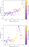 |
Fig. 13 Flow rates along the filaments in the active cube. The colour bar represents the velocity magnitude at that point. Top: 3D filament corresponding to filament 1 in Figure 3a. It feeds the central massive clump. Bottom: 3D filament representing filament 3 in Figure 3a. It feeds the non-central clump. Negative values represent positions leftwards of the clump, i.e., lower values of x and y. On the x-axis, 0 corresponds to the clump position. |
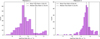 |
Fig. 14 Distributions of all the perpendicular flow rates measured at 0, π/2, π, and 3π/2 for the 3D filament spines in the active region. The dashed black and solid grey lines sit at the mean and median flow rate values, respectively, and the numbers are shown in the legend. Left: filament 1, which feeds the central massive clump. Right: filament 3, which feeds the non-central clump. |
6 Discussion
These results provide us with several key insights into the effect of the environment on the morphology and kinematics of filaments, and in particular, on the flow-rate trends we measured.
The highest flow rates of ∼10−1.5 M⊙yr−1 are found along the filaments in the quiet (less feedback-dominated) region (see Fig. 6). They are higher by over an order of magnitude (∼10−1.5 M⊙yr−1 vs. ∼10−3 M⊙yr−1) than the filamentary flow in filaments that are formed by the collision of superbubbles, which is characteristic of the active feedback-dominated region. This suggests that the spiral arms are more effective in funnelling material than the active region.
This is supported in Fig. 2, which plots the column densities of filaments in the two regions. The column density values are higher on average in the spiral arm (quiescent) region, suggesting higher flow rates. These higher column density regions are also more spatially extended from the clumps than the active region, where this intensity is concentrated in the clumps themselves. These two differences suggest that the dynamics of flows in spiral arms may play a more important role than stellar feedback in driving filament-aligned flow rates that feed gas into clumps and cluster-forming regions. Clearly, many more such regions, such as the central molecular zone (CMZ) or inter-arm regions, need to be examined before we can make firm conclusions and distinguish flows and structures in different galactic environments (see Pillsworth et al. 2025).
Several trends emerge from the measurements of the flow rates within the active and quiet cubes. The active cube exhibits a clear pattern in which the flow rates increase with the distance from the core, indicating that the flow dynamics are strongly affected by the feeder filaments near the hubs. These feeder filaments distribute the flow into multiple pathways, which reduces the flow rate in the central regions of the main filaments. Conversely, in the quiet cube, the flow rates are highest near the core and decrease with the distance, which suggests a more centralised accumulation of material. The distribution of feeder filaments along the main filaments in the quiet cube contributes to this pattern, as these feeders merge progressively and allow more material to reach the clump without significant distribution away from the central core.
The difference of about one order of magnitude in the median flow rates also suggests that a more dynamic process occurs closer to the central clumps in the active cube that is driven by multiple feeder filaments. In contrast, the higher median flow rate in the quiet cube indicates that even in regions of less feedback, a significant amount of material is still funnelled towards the central clumps.
Whilst we showed that using our observational method on the simulated data gives results that agree with the values derived directly from the models themselves, it is also important to compare the results with previous observational studies. Schneider et al. (2010) described the impact of filamentary structures on star formation with an in-depth study of the DR21 region and showed that flows onto the primary filaments can be enough to sustain them and their flow of material.
For a comparison to observational studies on similar scales to these simulations, we considered Beuther et al. (2020) and Rawat et al. (2024). Beuther et al. (2020) studied the flow rates in the cloud surrounding IRDC G28.3 at distances up to ~15 pc, similar to some of the filaments we studied. Their results are about 10−5 M⊙yr−1 and appear to be constant over the extent of the cloud. Rawat et al. (2024) identified and analysed six filaments in GMC G148.24+00.41. The lengths of the six filaments were 14–38 pc, and they calculated flow rates between 10−4 M⊙yr−1 and 10−5 M⊙yr−1.
Many other works included a flow-rate analysis along filaments or filamentary structures on different scales (e.g. Kirk et al. 2013; Henshaw et al. 2014; Wells et al. 2024) whose results agree with our observationally calculated results and simulation-based results.
Kumar et al. (2020) emphasised the role of hub-filament systems (HFSs) in star formation and concluded that hubs can trigger and drive longitudinal flows along the filaments in their systems. This fits the idea of feeder filaments and the two roles we detailed here well.
Zhang et al. (2024) studied filamentary sub-structure on much smaller scales than ours; ~0.17 pc. They reported flow rates at the higher end of our range, between ~1.8 × 10⁻⁴ M⊙yr−1 and ∼1.2 × 10⁻³ M⊙yr−1. The different scales of their filaments are a key factor here for the comparison with this work, which are about 20 pc in length. The authors also measured the flow rates within areas corresponding to the smallest scales covered by our simulations. Their values appear to lie at the upper end of our distributions, and additional small-scale effects, for instance, additional gravitational attraction, may increase their values.
These comparisons suggest that while broad trends and values are consistent in the studies, the detailed morphology and arrangement of filaments are key factors in the flow dynamics of star-forming regions, and it is of the upmost importance that we understand them. Future studies covering both larger and smaller spatial scales are needed to explore how these parameters vary with simulations and observations to shed further light on these issues.
7 Conclusions
Our analysis of the flow rates in different environmental conditions from a simulated Milky Way-type galaxy by Zhao et al. (2024) provided significant insights into the dynamics of filamentary structures in different star-forming environments. The use of FilFinder identification techniques allowed us to extract and analyse filaments. This revealed differences in the flow patterns between these regions. Overall, the flow rates were about 10−4 M⊙yr−1 and 10−5 M⊙yr−1, which agrees well with observations (e.g. Kirk et al. 2013; Henshaw et al. 2014; Beuther et al. 2020; Zhang et al. 2024; Wells et al. 2024). The key results are listed below:
The values for the observationally calculated flow rates along individual cuts onto the filaments are lower than those along the filament. The cumulative flow rates summed from these individual cuts along the filaments suffice to sustain the flow rates along the filaments;
In the active feedback-dominated region, the observational flow rates tend to increase with distance from the core. This pattern is explained by multiple feeder filaments within 1–2 pc of the central clump that distribute the flow into various paths onto the central clump;
The quiet more spiral-arm-like region displays higher observational flow rates towards the core. This suggests a more centralised accumulation of material. The progressive merging of feeder filaments into main filaments in these regions supports a sustained material flow towards the central clumps;
Radially around the clumps, we identified the primary filaments along with the presence or absence of feeder filaments, depending on the region. The primary filaments align with the directions of the largest radial contributions to the flow of material onto the clump;
Feeder filaments play distinct roles depending on the environment. In regions with higher feedback, they channel material from the primary filaments to feed the clumps. In contrast, in environments with less feedback, feeder filaments directly supply material from the surroundings to the primary filaments themselves;
Taking the average filament inclination for two of the filaments in the active region, we discussed that the observationally calculated values are slightly overestimated for filament 1, the filament that feeds the more massive clump, and they are underestimated by a factor of ∼72 for filament 3, which feeds the smaller clump in the region;
Our method for observationally estimating the flow rates produced results that agree with those directly from the simulation, with similar statistics and distributions. We are therefore confident in the values we were able to obtain using this method on observational data, but we note the effects of inclination and projection.
Finally, our findings agree numerically with observational studies. This highlights the critical role of filamentary structures in star formation. The differences in flow dynamics and filamentary structures underscore the importance of feeder filaments in shaping the star-forming environment. Future work should focus on refining simulations to match more observational scales and on exploring the effect of inclination on the observed flow rates.
Data availability
Interactive figures associated with Fig. 11 are available at https://www.aanda.org
Acknowledgements
The authors thank the referee for their helpful comments during the review of this manuscript. EWK acknowledges support from the Smithsonian Institution as a Submillimeter Array (SMA) Fellow. RP acknowledges support from an NSERC CGS-D scholarship. Some of the computational resources for this project were enabled by a grant to REP from Compute Canada/Digital Alliance Canada and carried out on the Cedar computing cluster. REP is supported with a Discovery grant from NSERC Canada.
References
- Alves, J., Zucker, C., & Goodman, A. 2020, Nature, 578 [Google Scholar]
- André, P., Men’shchikov, A., Bontemps, S., et al. 2010, A&A, 518, L102 [NASA ADS] [CrossRef] [EDP Sciences] [Google Scholar]
- André, P., Di Francesco, J., Ward-Thompson, D., et al. 2014, in Protostars and Planets VI, eds. H. Beuther, R.S. Klessen, C.P. Dullemond, & T. Henning, 27 [Google Scholar]
- Beuther, H., Wang, Y., Soler, J., et al. 2020, A&A, 638, A44 [NASA ADS] [CrossRef] [EDP Sciences] [Google Scholar]
- Bonnell, I. A., Bate, M. R., & Vine, S. G. 2003, MNRAS, 343, 413 [NASA ADS] [CrossRef] [Google Scholar]
- Bressert, E., Bastian, N., Gutermuth, R., et al. 2010, MNRAS, 409, L54 [NASA ADS] [Google Scholar]
- Chira, R. A., Kainulainen, J., Ibáñez-Mejía, J. C., Henning, T., & Mac Low, M. M. 2018, A&A, 610, A62 [NASA ADS] [CrossRef] [EDP Sciences] [Google Scholar]
- Clark, S. E., Peek, J. E. G., & Putman, M. E. 2014, ApJ, 789, 82 [NASA ADS] [CrossRef] [Google Scholar]
- Duan, X., & Guo, F. 2024, ApJ, 972, 41 [Google Scholar]
- Federrath, C., Rathborne, J. M., Longmore, S. N., et al. 2016, ApJ, 832, 143 [NASA ADS] [CrossRef] [Google Scholar]
- Fiege, J. D., & Pudritz, R. E. 2000, MNRAS, 311, 105 [NASA ADS] [CrossRef] [Google Scholar]
- Goldsmith, P. F., Heyer, M., Narayanan, G., et al. 2008, ApJ, 680, 428 [Google Scholar]
- Gómez, G. C., & Vázquez-Semadeni, E. 2014, ApJ, 791, 124 [Google Scholar]
- Grudić, M. Y., Kruijssen, J. M. D., Faucher-Giguère, C.-A., et al. 2021, MNRAS, 506, 3239 [NASA ADS] [CrossRef] [Google Scholar]
- Hacar, A., Tafalla, M., Forbrich, J., et al. 2018, A&A, 610, A77 [NASA ADS] [CrossRef] [EDP Sciences] [Google Scholar]
- Hacar, A., Clark, S. E., Heitsch, F., et al. 2023, in Astronomical Society of the Pacific Conference Series, 534, Protostars and Planets VII, eds. S. Inutsuka, Y. Aikawa, T. Muto, K. Tomida, & M. Tamura, 153 [Google Scholar]
- Hacar, A., Konietzka, R., Seifried, D., et al. 2025, A&A, 694, A69 [NASA ADS] [CrossRef] [EDP Sciences] [Google Scholar]
- Haid, S., Walch, S., Seifried, D., et al. 2019, MNRAS, 482, 4062 [NASA ADS] [CrossRef] [Google Scholar]
- Henshaw, J. D., Caselli, P., Fontani, F., Jiménez-Serra, I., & Tan, J. C. 2014, MNRAS, 440, 2860 [Google Scholar]
- Hillel, S., & Soker, N. 2020, ApJ, 896, 104 [Google Scholar]
- Jackson, J. M., Finn, S. C., Chambers, E. T., Rathborne, J. M., & Simon, R. 2010, ApJ, 719, L185 [Google Scholar]
- Kim, J.-h., Agertz, O., Teyssier, R., et al. 2016, ApJ, 833, 202 [NASA ADS] [CrossRef] [Google Scholar]
- Kirk, H., Myers, P. C., Bourke, T. L., et al. 2013, ApJ, 766, 115 [Google Scholar]
- Koch, E. W., & Rosolowsky, E. W. 2015, MNRAS, 452, 3435 [Google Scholar]
- Krumholz, M. R. 2014, Phys. Rep., 539, 49 [Google Scholar]
- Kumar, M. S. N., Palmeirim, P., Arzoumanian, D., & Inutsuka, S. I. 2020, A&A, 642, A87 [EDP Sciences] [Google Scholar]
- Lada, C. J., & Lada, E. A. 2003, ARA&A, 41, 57 [Google Scholar]
- Li, P. S., & Klein, R. I. 2019, MNRAS, 485, 4509 [NASA ADS] [CrossRef] [Google Scholar]
- Mullens, E., Zucker, C., Murray, C. E., & Smith, R. 2024, ApJ, 966, 127 [Google Scholar]
- Myers, P. C. 2009, ApJ, 700, 1609 [Google Scholar]
- Nunez-Iglesias, J., Blanch, A., Looker, O., Dixon, M., & Tilley, L. 2018, PeerJ, 6, 4312 [Google Scholar]
- Olivares, V., Salome, P., Combes, F., et al. 2019, A&A, 631, A22 [NASA ADS] [CrossRef] [EDP Sciences] [Google Scholar]
- Padoan, P., Pan, L., Juvela, M., Haugbølle, T., & Nordlund, Å. 2020, ApJ, 900, 82 [NASA ADS] [CrossRef] [Google Scholar]
- Pillsworth, R., & Pudritz, R. E. 2024, MNRAS, 528, 209 [NASA ADS] [CrossRef] [Google Scholar]
- Pillsworth, R., Roscoe, E., Pudritz, R. E., & Koch, E. W. 2025, arXiv e-prints [arXiv:2504.01099] [Google Scholar]
- Pineda, J. E., Arzoumanian, D., Andre, P., et al. 2023, in Astronomical Society of the Pacific Conference Series, 534, Protostars and Planets VII, eds. S. Inutsuka, Y. Aikawa, T. Muto, K. Tomida, & M. Tamura, 233 [Google Scholar]
- Ragan, S. E., Henning, T., Tackenberg, J., et al. 2014, A&A, 568, A73 [NASA ADS] [CrossRef] [EDP Sciences] [Google Scholar]
- Rawat, V., Samal, M. R., Walker, D. L., et al. 2024, MNRAS, 528, 2199 [NASA ADS] [CrossRef] [Google Scholar]
- Russell, H. R., McDonald, M., McNamara, B. R., et al. 2017, ApJ, 836, 130 [NASA ADS] [CrossRef] [Google Scholar]
- Schisano, E., Molinari, S., Elia, D., et al. 2020, MNRAS, 492, 5420 [Google Scholar]
- Schneider, N., Csengeri, T., Bontemps, S., et al. 2010, A&A, 520, A49 [CrossRef] [EDP Sciences] [Google Scholar]
- Svoboda, B. E., Shirley, Y. L., Traficante, A., et al. 2019, ApJ, 886, 36 [Google Scholar]
- Turk, M. J., Smith, B. D., Oishi, J. S., et al. 2011, ApJS, 192, 9 [NASA ADS] [CrossRef] [Google Scholar]
- Urquhart, J. S., König, C., Giannetti, A., et al. 2018, MNRAS, 473, 1059 [Google Scholar]
- Wells, M. R. A., Beuther, H., Molinari, S., et al. 2024, A&A, 690, A185 [NASA ADS] [CrossRef] [EDP Sciences] [Google Scholar]
- Xu, X., Li, D., Dai, Y. S., Goldsmith, P. F., & Fuller, G. A. 2020, ApJ, 898, 122 [Google Scholar]
- Xu, X., Wang, K., Gou, Q., et al. 2024, MNRAS, 535, 940 [Google Scholar]
- Zhang, S., Cyganowski, C. J., Henshaw, J. D., et al. 2024, MNRAS, 533, 1075 [Google Scholar]
- Zhao, B., Pudritz, R. E., Pillsworth, R., Robinson, H., & Wadsley, J. 2024, ApJ, 974, 240 [NASA ADS] [CrossRef] [Google Scholar]
- Zhou, J. W., Dib, S., & Davis, T. A. 2024, MNRAS, 534, 683 [NASA ADS] [CrossRef] [Google Scholar]
- Zinnecker, H. 1984, MNRAS, 210, 43 [Google Scholar]
- Zucker, C., & Chen, H. H.-H. 2018, ApJ, 864, 152 [NASA ADS] [CrossRef] [Google Scholar]
- Zucker, C., Battersby, C., & Goodman, A. 2015, ApJ, 815, 23 [NASA ADS] [CrossRef] [Google Scholar]
- Zucker, C., Goodman, A., Alves, J., et al. 2021, ApJ, 919, 35 [NASA ADS] [CrossRef] [Google Scholar]
The astro-analysis code is found here: https://github.com/yt-project/yt_astro_analysis
All Tables
All Figures
|
Fig. 1 Galaxy overview from Zhao et al. (2024). The central panels show the two snapshots of the galaxy we used, the top panel shows the location of the region with less feedback (quiet), and the bottom panel shows the location of the feedback-dominated region (active). The first zoom-in panels show the regions down to a few kiloparsec (top left and bottom right panels), followed by the close-ups of the regions in 100 × 100 pc boxes (bottom left and top right panels). |
| In the text | |
|
Fig. 2 Density projections of high-resolution zoom-in simulation data of Zhao et al. (2024). The white streamlines represent the magnetic field structure. The arrows show velocity direction and magnitude relative to the velocity of the central cores in each snapshot. |
| In the text | |
|
Fig. 3 Zeroth-moment maps of the column density cubes with the identified filamentary structure, colour-coded by velocity, are overlaid. The 2.85 pc scale bars are shown in the top right corners. |
| In the text | |
|
Fig. 4 Zeroth-moment map of the active column density cube with the identified filamentary structure, colour-coded by velocity, is overlaid. The green, red, and blue points indicate the different types of the flow rate. Green is along the filamentary structure, red is onto, and blue is polar around the clumps. The 2.85 pc scale bar is shown in the top right corner. |
| In the text | |
|
Fig. 5 Distributions of the flow rates. Left: along filaments. Right: onto the filaments in the active cube. |
| In the text | |
|
Fig. 6 Distributions of the flow rates. Left: along filaments. Right: onto the filaments in the quiet cube. |
| In the text | |
|
Fig. 7 Distance vs. flow rate in log space and relation for each filament in the active cube (filaments are labelled in Fig. 3a), colour-coded by velocity difference. |
| In the text | |
|
Fig. 8 Distance vs flow rate in log space, and relation for each filament in the quiet cube (filaments are labelled in Fig. 3a), colour-coded by the velocity difference. |
| In the text | |
|
Fig. 9 Relation of radial distance to the flow rate for eight different angles around each clump in the active region. Numbers from 0.5 to 3.5 represent the distance from the centre for each of the concentric circles in pc. The dashed red lines indicate the primary filaments, and the solid blue lines indicate the directions of the feeder filaments. |
| In the text | |
|
Fig. 10 Relation of the radial distance to the flow rate for eight different angles around each clump in the quiet region. Numbers from 0.5 to 3.5 represent the distance from the centre for each of the concentric circles in pc. The dashed red lines indicate the primary filaments, and the solid blue lines indicate the directions of the feeder filaments. |
| In the text | |
|
Fig. 11 3D projection of the filament spines for filaments 1 (top) and 3 (bottom) in the active cube. The colour bar shows the parallel flow rate at that point in the spine, and the grey markers depict the points for which the direction vector of the spine was null. The light purple plane surface shows the position of the galaxy midplane. An interactive version of this figure is available in the online version of this paper. |
| In the text | |
|
Fig. 12 Effect of the galactic inclination on the relation of distance vs. flow rate in log space for filament 1 from the active region. The results are shown for five different galactic inclinations of 0, 20, 45, 70, and 90 degrees. |
| In the text | |
|
Fig. 13 Flow rates along the filaments in the active cube. The colour bar represents the velocity magnitude at that point. Top: 3D filament corresponding to filament 1 in Figure 3a. It feeds the central massive clump. Bottom: 3D filament representing filament 3 in Figure 3a. It feeds the non-central clump. Negative values represent positions leftwards of the clump, i.e., lower values of x and y. On the x-axis, 0 corresponds to the clump position. |
| In the text | |
|
Fig. 14 Distributions of all the perpendicular flow rates measured at 0, π/2, π, and 3π/2 for the 3D filament spines in the active region. The dashed black and solid grey lines sit at the mean and median flow rate values, respectively, and the numbers are shown in the legend. Left: filament 1, which feeds the central massive clump. Right: filament 3, which feeds the non-central clump. |
| In the text | |
Current usage metrics show cumulative count of Article Views (full-text article views including HTML views, PDF and ePub downloads, according to the available data) and Abstracts Views on Vision4Press platform.
Data correspond to usage on the plateform after 2015. The current usage metrics is available 48-96 hours after online publication and is updated daily on week days.
Initial download of the metrics may take a while.