| Issue |
A&A
Volume 704, December 2025
|
|
|---|---|---|
| Article Number | A22 | |
| Number of page(s) | 12 | |
| Section | Stellar structure and evolution | |
| DOI | https://doi.org/10.1051/0004-6361/202555524 | |
| Published online | 26 November 2025 | |
Detailed theoretical analysis of core Helium-burning stars: Mixed mode patterns
I. Impact of the He-flash discontinuity and of induced semi-convection
1
STAR Institute, Université de Liège, Liège, Belgium
2
Department of Physics & Astronomy “Augusto Righi”, University of Bologna, Via Gobetti 93/2, 40129 Bologna, Italy
3
INAF-Astrophysics and Space Science Observatory of Bologna, Via Gobetti 93/3, 40129 Bologna, Italy
⋆ Corresponding author: This email address is being protected from spambots. You need JavaScript enabled to view it.
Received:
15
May
2025
Accepted:
2
October
2025
Abstract
Context. Recent space missions such as CoRoT, Kepler, and TESS have made asteroseismology a powerful tool for studying the internal structure of stars. Red giants, in particular, are central in these studies due to their rich oscillation spectra, which provide details of both their core and envelope through their mixed oscillation modes. Despite these advances, models of core helium-burning red giants struggle to reproduce the observed oscillation spectra, particularly because of uncertainties in the treatment of mixing processes such as overshooting and semi-convection. These discrepancies highlight the need for further asteroseismic constraints to improve stellar models.
Aims. We aim to identify the key structural features influencing asteroseismic observations and how seismic signatures relate to internal chemical composition by investigating the asteroseismic properties of core helium-burning stars with a consistent treatment of induced semi-convection and overshooting.
Methods. We use a new version of the Liège stellar evolution code and the Liège adiabatic oscillation code to compute and analyse the mixed-mode oscillation patterns of various models of core helium-burning stars.
Results. We find that sharp transitions in the chemical composition and overshooting in the central part of the models significantly affect the mixed-mode oscillation spectra of core helium-burning stars. Overshooting variations alter the size of the semi-convective zone, which locally modifies the Brunt–Väisälä frequency and, thereby, the observed period spacing. Notably, our models indicate that modifications in overshooting are balanced by adjustments in the semi-convective layers, maintaining a consistent total mixed-core size across models. Thus, stellar evolution is minimally affected by these internal adjustments, unlike the seismic signatures, as seen in the Brunt–Väisälä frequency profile. The semi-convective zone also introduces additional seismic trapping, although for advanced models, modes confined within this region are unlikely to be detectable due to their high energy density and minimal impact on surrounding modes.
Conclusions. We highlight the importance of detailed seismic studies to characterise mixing processes near the convective core in core helium-burning stars. This provides a first step towards constraining the chemical composition gradient. In addition, we notice a balance between the extension of overshooting and semi-convective zones, affecting the oscillation spectra.
Key words: asteroseismology / stars: evolution / stars: interiors
© The Authors 2025
 Open Access article, published by EDP Sciences, under the terms of the Creative Commons Attribution License (https://creativecommons.org/licenses/by/4.0), which permits unrestricted use, distribution, and reproduction in any medium, provided the original work is properly cited.
This article is published in open access under the Subscribe to Open model. This email address is being protected from spambots. You need JavaScript enabled to view it. to support open access publication.
1. Introduction
In recent decades, high-quality data from space missions such as CoRoT (Auvergne et al. 2009), Kepler (Borucki et al. 2010), and TESS (Ricker et al. 2014) have established asteroseismology as a powerful tool for probing the internal structure and dynamics of stars. It has been particularly efficient in analysing the rich seismic spectra of red giant (RGB) stars (see e.g. Chaplin & Miglio 2013; Hekker & Christensen-Dalsgaard 2017, and references therein). In RGBs, pressure modes (p modes) are acoustic waves that mainly propagate in the extended convective envelope, where pressure is the dominant restoring force. Gravity modes (g modes), on the other hand, are buoyancy-driven and propagate in the dense radiative core. Because RGBs have both a compact core and an extended envelope, some oscillations become mixed modes – behaving as g modes in the core and p modes in the envelope – which allows us to probe both regions. Red giant stars serve as laboratories for testing the theory of stellar structure and evolution, exposing several issues with theoretical models (Siess 2009; Lagarde et al. 2011; Mosser et al. 2012; Deheuvels et al. 2014; Pinçon et al. 2020). One major achievement of their seismic study has been the ability to distinguish between different evolutionary stages of RGBs, namely hydrogen-shell burning and core-helium burning (CHeB) stars (Montalbán et al. 2010; Bedding et al. 2011; Mosser et al. 2011). This distinction was made possible by the difference in the density contrast between the core and the average density. The onset of nuclear reactions reduces the central density in a CHeB star by almost a factor of 10 compared to that of an RGB star. This shifts the region that contributes the most to the Brunt–Väisälä frequency to larger radii, with a clear effect on the value of the period spacing (Montalbán et al. 2013). Moreover, this different density contrast modifies the coupling between the g- and p-mode cavities, affecting – among other things – the regularity of the spectrum (Montalbán et al. 2010).
Furthermore, a significant discrepancy of two orders of magnitude was revealed between the predicted core rotation of RGBs in both evolutionary stages and theoretical stellar models (Mosser et al. 2012, 2024a; Eggenberger et al. 2012; Marques et al. 2013; Deheuvels et al. 2015; Gehan et al. 2018). Theoretical models incorporating additional transport processes predict a spin-up of the core as CHeB proceeds (Moyano et al. 2022, 2023), contrary to recent observations by Mosser et al. (2024a).
In addition, numerous studies have highlighted the need for additional mixing at the border of convective regions, for example at the base of the convective zone in H-shell-burning RGB stars (Lagarde et al. 2012; Khan et al. 2018) or at the top of the convective core of main-sequence stars with masses higher than ≈1.2 M⊙ (Claret & Torres 2016, 2019; Deheuvels et al. 2016; Viani & Basu 2020; Noll et al. 2021; Noll & Deheuvels 2023; Lindsay et al. 2024, amongst others). During core helium burning, a similar situation occurs with the presence of a growing convective core, the evolution of which may be altered by additional mixing at its border (Montalbán et al. 2013; Bossini et al. 2015; Vrard et al. 2022; Dréau et al. 2022). Despite the importance of core helium-burning stars for understanding chemical mixing, since their cores are sites of convective motions, the complexity of their oscillation spectra has hindered detailed studies on these promising targets. Computing models suitable for detailed asteroseismic applications during this evolutionary phase is challenging, notably due to sharp variations in the structure of the inner core (Vrard et al. 2022), which create glitch signatures (see Cunha et al. 2015, 2019, 2024, for analytical developments and theoretical discussions on buoyancy glitches) in their seismic spectra, compounded by the problem of semi-convection (see e.g. Salaris & Cassisi (2017) and references therein). Some studies have even examined the seismic properties of stars undergoing “helium flashes” (Deheuvels & Belkacem 2018). Extracting valuable information from asteroseismic data requires advancing our understanding of the processes generating the observed signals and determining the most relevant seismic constraints to accurately infer the internal structure. Therefore, additional mixing processes such as convective overshooting and semi-convection have yet to be characterised for this evolutionary phase using detailed asteroseismic analyses.
In this context, we present theoretical asteroseismic applications of a new version of the Liège stellar evolution code (CLES, Scuflaire et al. 2008) for evolutionary models of CHeB stars with different initial parameters, where their mode frequencies are computed with the Liège adiabatic oscillation code (LOSC, Scuflaire et al. 2008). The evolution code provides a consistent treatment of semi-convection. It also ensures a high degree of consistency in verifying hydrostatic equilibrium and treating convective boundaries, enabling detailed asteroseismic analyses. Our aim is to establish a framework for a detailed asteroseismic analysis of CHeB stars, with the goal of providing additional insights into the theoretical models currently used in stellar evolution codes and hydrodynamical simulations (e.g. Mirouh et al. 2012; Cristini et al. 2016; Rizzuti et al. 2022; Blouin et al. 2024, amongst other). In particular, we aim to investigate how the asteroseismic properties of these stars are influenced by semi-convective and overshooting processes, focusing on the connection between seismic signatures and internal chemical composition. Notably, our study examines mode trapping caused by sharp structural variations. A trapping region is defined as a zone where an oscillation mode remains confined – with large amplitudes inside and rapidly decreasing outside – bounded by turning points where reflection occurs (see e.g. Takata 2016, for a discussion of dipolar mixed oscillation modes).
Modelling low-mass RGBs in the CHeB phase presents significant challenges due to their complex internal structure. These difficulties become particularly evident after the initial stage of CHeB, when a semi-convective layer emerges. The treatment of this region in stellar evolution computations requires us to manage the “semi-convection problem”. We recall that a region undergoing convective motions is characterised by the Schwarzschild criterion ∇ad < ∇rad, which expresses convective instability due to a high temperature gradient through the radiative and adiabatic gradients, defined in Sect. 3. To ensure a coherent model, the boundary of the convective core must satisfy the condition that the resulting force (hence acceleration) vanishes; that is, ∇ad = ∇rad on the convective side of the boundary. In CLES, we follow the prescriptions described in Gabriel et al. (2014). Beyond the location of the core boundary, an additional region affected by convective elements may appear. This so-called overshooting region is also a critical issue in modelling main sequence stars that exhibit a convective core. The challenge in modelling a CHeB star lies notably in handling the growth of the convective core and the appearance of the semi-convective zone (e.g. Castellani et al. 1985; Straniero et al. 2003; Serenelli & Weiss 2005; Noels 2013). As discussed in Salaris & Cassisi (2017) and analysed in the work of Castellani et al. (1971a), the initial phase of CHeB is characterised by a convective core, whose mass grows with time due to the increase in opacity as helium is transformed into carbon and oxygen. The radiative gradient develops a minimum located inside the fully mixed core, which lies at the root of the semi-convection problem. In practical terms, this minimum leads to an ambiguous boundary for the convective core, as the radiative gradient increases beyond the point of neutrality. Salaris & Cassisi (2017) provides a visualisation of the gradient profile in their Section 4.2, as well as in their Figs. 8 and 9. We also refer to Castellani et al. (1971b, 1972), Castellani & Tornambe (1982), Straniero et al. (2003), Giammichele et al. (2018) for additional references on the evolution of convective cores during CHeB and to Girardi (2016) for a recent review.
In Sect. 2, we present our stellar models as well as details on the formalism used in the stellar evolution code to cover this stage of evolution. We introduce the global asteroseismic parameters in Sect. 3 and present the seismic signatures of internal structural variations during the evolution, related to mixing processes such as convection and semi-convection. In the last section (Sect. 4), we analyse the oscillation spectra of various models to provide an overview of the expected asteroseismic signatures arising from our treatment of semi-convection and overshooting across the range of model parameters considered.
2. Stellar evolution models
2.1. Liège Stellar Evolution Code (CLES)
In CLES (Scuflaire et al. 2008), a semi-convective zone appears above the overshooting region (whenever overshooting of convective elements is considered). The base of the semi-convective region is located beyond the minimum of the radiative gradient at the point where it reaches the adiabatic gradient. By adjusting the chemical composition, this semi-convective region ensures that the neutrality condition ∇ad = ∇rad is satisfied from that point up to the discontinuity boundary, creating a chemically variable profile. This approach known as “induced semi-convection” is similar to the methods used in other stellar evolution codes (Ventura et al. 2008; Degl’Innocenti et al. 2008; Bressan et al. 2013) and is the one implemented in our code.
Since its original publication in 2008 (Scuflaire et al. 2008), the software has undergone numerous updates. In this new version, we adopted the same strategy for the helium-burning phase and developed a new branch dedicated to it. We did not include the descriptions of phenomena unlikely to alter our conclusions, such as mass loss and diffusion, so that we could focus our attention and efforts on convergence problems and describing the semi-convective zone. In this way, we were able to test different prescriptions for the composition and boundaries of the semi-convective zone.
Although the helium combustion reactions were coded in the original version of CLES, this version was not suitable for calculating these evolutionary phases, and the calculation was stopped as soon as helium combustion began. The rest of the evolution is based on two programs, ZAHB and HBevol. If the mass of the model is sufficient to avoid helium flash, the rest of the evolution is handled by the HBevol program. For smaller masses, we began just after the flash using ZAHB (zero age horizontal branch) to calculate an initial static model that would serve as the starting point for HBevol. These initial models were inspired by the properties of ATON evolutionary models (Ventura et al. 2008), which were used in the phases of initial development.
The ZAHB program computes a static stellar model intended to represent the star immediately after the helium flash. This approach is justified by the fact that, during the central helium-burning phase, the gravitational energy contribution is negligible compared to the nuclear term. The model is defined by the usual parameters – total mass, initial hydrogen and metal fractions (X, Z), convection, and overshooting – together with two core parameters that determine its internal properties: the helium core mass (mHe) and the carbon enrichment of the helium core (XCO) produced during the flash. In fully evolutionary computations, these parameters are direct outputs of stellar evolution, but here they are treated as free parameters defining the initial conditions for the CHeB phase.
The parameter mHe generally lies between 0.45 and 0.50 M⊙; as a first step, we fixed it to 0.50 M⊙, close to values found in evolutionary models (Girardi 2016). A later step in our work consists of calibrating this value from full evolutionary calculations. By keeping the mass of the helium core constant while varying the total mass, our approach essentially corresponds to physically altering the envelope mass of the models and computing their evolution right after they have undergone the flash. This approach allows us to reduce the complexity of the analysis and focus on the effects of the other free parameters. The second parameter, XCO, denotes the mass fraction of helium converted to carbon through the triple-alpha nuclear reaction. In our modelling approach, this results in a small discontinuity in chemical composition, located below the hydrogen-burning shell, attributed to the remnant of the “helium-flash” (Kippenhahn & Weigert 2013).
2.2. Models computation
The stellar models used in this study were computed with CLES using the FreeEOS equation of state (Irwin 2012). Their initial properties were as follows: The CHeB models we computed were at solar metallicity, taken from Asplund et al. (2009). The mass fraction of hydrogen and metallicity at the surface were fixed at 0.72 and 0.014, respectively. Inside the core, the mass fraction of carbon, determined by the parameter XCO, was set at 0.05 at the beginning of our computations.
The mass of the helium core is a free parameter initially fixed at mHe = 0.50 M⊙ for all our models; thereafter, CLES computes the evolution coherently. Opacities were taken from type II OPAL tables (Iglesias & Rogers 1996), supplemented at low temperature by the Wichita State University opacities (Ferguson et al. 2005). Our models exhibit a convective core surrounded by an overshooting layer, a semi-convective layer modelled using induced-convection, a hydrogen-burning shell, and a convective envelope modelled by means of the mixing length theory (Weiss et al. 2004) with a solar-calibrated mixing length of l = 1.8 HP, where  is the pressure scale height. The radial extent of the penetrative convection region (Zahn 1991), which undergoes instantaneous mixing and has the temperature gradient set to the adiabatic one (Maeder 1975), is initially set as d = αov HP, where αov denotes the overshooting parameter, a free parameter in the code. At the surface, the models have a grey Eddington atmosphere.
Discontinuity in the chemical composition due to the depletion of helium (XCO) associated with the helium-flash creates a sharp transition in the helium profile around 0.5 m/M, as illustrated in Fig. 1. We reiterate that XCO is a free parameter in our code but can be calibrated using consistent evolutionary computations. In our case, to maintain greater flexibility in our investigations, we keep it as a free parameter throughout the computations.
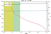 |
Fig. 1. Gradient profile as a function of mass fraction for a one-solar-mass CHeB star at solar metallicity and Yc = 0.90. The helium profile is shown in parallel (black). The convective zone is in yellow; the overshooting layer is in green; and the sharp variation left by the “He flash” is in grey with XCO = 5%. The radiative gradient ∇rad is in red, and the adiabatic gradient ∇ad in blue. The real gradient ∇ is defined as follows: ∇ = ∇ad in the COS zone, and ∇ = ∇rad in the radiative zone. We focus on the central part of the star for illustrative purposes. |
In the following sections, we refer to the three central zones (convective core, overshooting, and semi-convective layers) collectively as the “COS” zone, and the combination of the convective core and the overshooting layer as the “fully mixed” core. The evolutionary track of our models in the Hertzsprung–Russell diagram follows a similar pattern to that of CHeB star evolutionary models with masses ranging from 1 M⊙ to 1.5 M⊙1 (see e.g. Girardi 2016, for a review) as illustrated in the top panel of Fig. 2. The total luminosity gradually decreases on the horizontal branch, while the effective temperature remains almost constant. At around Yc = 0.40, a turn-around occurs in the track, and the luminosity begins to increase. This characteristic may be sensitive to the treatment of convective overshooting or other mixing processes. For comparison, it occurs at Yc ∼ 0.30 in Montalbán et al. (2013), and around Yc ∼ 0.75 in Constantino et al. (2015). These differences highlight the need for further investigation, especially given the uncertainties associated with the treatment of the mixed regions close to the helium-burning core and the way the Schwarzschild criterion is applied in various evolutionary computations (Gabriel et al. 2014). During this phase, luminosity originates from two main sources of energy: the H-burning shell surrounding the He core and the helium burning at the centre. As helium is transformed into carbon in the core, the opacity increases, which results in an increase in the radiative gradient and the convective core mass. The temperature sensitivity of the 3α reactions is so large that it imposes a decrease in density (Kippenhahn et al. 2012). The reactions are influenced by the production of oxygen, with the reaction 12C(α, γ)16O becoming progressively dominant. Simultaneously, the H shell fades away, causing a decrease in the surface luminosity. When Yc drops to around 0.40, the central density begins to increase, as shown in the ρc − Tc diagram in the bottom panel of Fig. 2. This turn-around is linked to the appearance of a semi-convective layer, since it limits the growth of the fully mixed core in our models. This changes the amount of mass incorporated into the convective core, which influences the nuclear reactions as modelled in CLES (Angulo et al. 1999; Kunz et al. 2002), thereby affecting the evolution of the core and the central density.
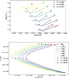 |
Fig. 2. Top panel: Evolutionary track in the Hertzsprung–Russell diagram of the sequence of models from 1 M⊙ to 1.5 M⊙ stellar masses at fixed He-core mass. The markers indicate the state of central helium abundance studied: Yc = 0.90, Yc = 0.40, and Yc = 0.10. Bottom panel: Central temperature as a function of the central density in logarithmic scale for the corresponding set of masses. |
The core contraction raises the temperature in the shell, increasing the nuclear rate of hydrogen burning and increasing both shell and surface luminosity. As the core attains a helium abundance of Yc = 0.10, the production of oxygen becomes increasingly important. Moreover, the contribution of the 3α reaction simultaneously decreases, causing the core to contract further and the envelope to expand.
The induced semi-convection method implemented in CLES imposes the chemical composition gradient to obtain the neutrality condition of the gradients ∇ad = ∇rad. This is done by allowing partial chemical mixing just enough to equalize the radiative gradient with the adiabatic value and imposing conservation of the total mass of each chemical element (apart from nuclear reactions). Although this provides a consistent framework for modelling the semi-convective regions in core-helium-burning stars, our understanding and modelling of the underlying physical processes remain incomplete. Various approaches, such as the 3D hydrodynamic simulations in Wood et al. (2013), may be considered to address this issue. More recent studies, such as Blouin et al. (2024), examine the stability of semi-convective layers, while Fuentes (2025) investigate the effects of rotation on semi-convective transport, specifically in the context of Jupiter. While these simulations provide insights into the dynamics of semi-convection, they remain subject to some limitations. They are not tested against observational constraints or carried out in fully stellar conditions (e.g. thermal relaxation over evolutionary timescales). Moreover, some might not include physical processes such as rotation and magnetism, which could alter mixing efficiency. These studies and their different conclusions regarding semi-convective regions highlight the need for further investigations into stellar interiors. A complementary approach involves using seismic constraints to extract detailed information about the internal structure and mixing processes in these regions, leveraging the information provided by individual oscillation modes – this being the primary focus of our study.
3. Global asteroseismic indicators
According to asymptotic theory, global seismic indicators can be defined for both p and g modes, see Shibahashi (1979), Tassoul (1980), and Takata (2016) for mixed oscillation modes. The large frequency separation is expressed as
 (1)
(1)
with c being the local sound speed; the integral representing the acoustic radius; and r and R denoting the local radial coordinate and the stellar radius, respectively. ℓ and n represent the degree of spherical harmonics and the radial overtone, respectively. The asymptotic large frequency separation, commonly used in RGBs, is a constant defined from radial modes, which are pure p modes corresponding to ℓ = 0 (see Mosser et al. 2013, for a discussion).
Gravity-dominated mixed modes are typically associated with quasi-equidistant periods, defined as the period spacing:
 (2)
(2)
with N, the Brunt-Väisälä frequency, defined as
 (3)
(3)
Here g is the local gravitational acceleration; and 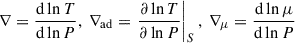 are the temperature gradient, the adiabatic temperature gradient, and the mean molecular weight, respectively. We compute the integral only in regions where N2 is higher than zero.
The large frequency separation of radial modes (ℓ = 0) does not vary in the asymptotic regime. Hereafter, we treat this asymptotic value as constant and denote it as Δν. Similar behaviour is expected from the period spacing of dipolar modes in the asymptotic regime; thus, we define an asymptotic period spacing of dipolar modes (ℓ = 1), denoted ΔΠ, which are used to study the properties of our models. Both quantities are global seismic indicators commonly used when studying RGBs, as they are often determined with a high degree of precision (typically of the order of 0.1 μHz for Δν and ≈3 s for ΔΠ as in Vrard et al. 2022; Mosser et al. 2024b). In our grid of models, these parameters can be analysed throughout the entire evolutionary sequence. Internal structural variations, particularly those affecting the chemical gradient, influence the gravity-mode cavity of mixed modes.
We begin by analysing the global asymptotic seismic parameters of a selected grid of models of mass 1 M⊙ with αov = 0.50 using the seismic diagram Δν − ΔΠ shown in Fig. 3a. Starting from early stages of the horizontal branch, where Yc is approximately 0.90, and continuing to a value around Yc = 0.40, the asymptotic period spacing ΔΠ increases significantly, consistent with previous studies using evolutionary models (see e.g. Montalbán et al. 2013; Bossini et al. 2015; Constantino et al. 2015). Beyond this state, a turn-around in the track appears where it begins to decrease until the end of the sequence. This is similar to what is observed in the evolutionary tracks in the top panel of Fig. 2 when the core contracts. In this case, the dependence on the radius r and the evolution of the Brunt-Väisälä frequency profile can explain this trend in the period-spacing. As mentioned in Eq. (3), N strongly depends on the factor ρg2/P that guides variations in period spacing as the core expands or contracts.
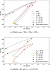 |
Fig. 3. Top panel: Diagram Δν − ΔΠ of three models of different stellar mass. Each point corresponds to a stage (Yc) in the evolution on the horizontal branch. The markers indicate the state of central helium abundance (Yc = 0.90, Yc = 0.40, and Yc = 0.10) and the appearance of the semi-convective layer. Bottom panel: Diagram Δν − ΔΠ of two models with different overshooting parameters αov. |
In the COS zone, ∇ is equal to the adiabatic gradient (∇ad = ∇) (see Fig. 4a for the gradient profile), and the chemical composition gradient vanishes in the fully mixed region due to efficient mixing, interpreted as a result of convection (∇μ = 0). Consequently, the Brunt-Väisälä frequency vanishes in the fully mixed core but maintains a non-zero profile throughout the semi-convective zone and radiative parts of the star. As the models evolve and the abundance reaches Yc = 0.40, the core slows its expansion and, at some point, contracts rapidly, as discussed above in relation to the increasing central density shown in the lower panel of Fig. 2. This trend change affects asymptotic period spacing as the factor ρg2/P increases and the radius r decreases. It draws a turn-around in the track around Yc = 0.40, as shown in Fig. 3.
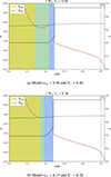 |
Fig. 4. Comparison of overshooting parameters αov = 0.50 (top panel) and αov = 0.15 (bottom panel) for 1 M⊙ through the gradient and helium profiles as a function of the mass fraction at the same age, compared to the helium profile (black). The convective zone is in yellow; the overshooting layer is in green; the semi-convective zone is in blue; and the sharp variation left by the He-flash is in grey. The radiative gradient ∇rad is in red, and the adiabatic gradient ∇ad is in blue. The real gradient ∇ is defined as follows: ∇ = ∇ad in the COS zone, and ∇ = ∇rad in the radiative zone. |
To analyse the impact on seismic indicators, we conduct our next investigation using a set of models with various stellar masses. The study of a slightly higher mass reveals the same general trend in period spacing as observed for 1 M⊙. In Fig. 3a, we select 1.1 and 1.2 M⊙ models as comparative examples and observe that their tracks exhibit roughly the same initial ΔΠ at a given Δν, reflecting the similar size of their helium cores. The central propagation cavities thus exhibit the same structure at this particular stage, resulting in similar N and Δν profiles. We also notice that during the evolution, the tracks diverge while the asymptotic period spacing increases. For a given value of Δν, a lower mass star exhibits higher ΔΠ, since the value of ρc − Tc is different for each mass. The tracks change direction at approximately the same central helium abundance, ∼Yc = 0.40, for each model. This corresponds to the same effect discussed in the evolutionary tracks of Fig. 2, where the change in temperature sensitivity of the central nuclear reactions leads to an increase in the central density.
Another stellar parameter that significantly impacts the global seismic indicators is the overshooting layer. It extends from the convective core, where ∇rad > ∇ad. Size variations in αov also affect the size of the semi-convective layer in the computed models. Interestingly, the semi-convective layer appears to compensate for variations in αov, such that a larger overshooting layer corresponds to a smaller semi-convective region, and vice versa. Fig. 4 illustrates this trend in parallel to the chemical composition profile. When the semi-convective layer appears, the Yc is also affected, with a delayed appearance in models with large overshooting. For models of the same age across the sequence, their helium central abundance is very similar. We observe that the total size of the mixed core remains relatively similar once the semi-convective parameter is present, even if the initial extent of overshooting is modified.
The profile of the Brunt-Väisälä frequency undergoes sharp transitions at the bottom and top of the semi-convective region (blue zone in Fig. 4), while it is zero in the convective core and in the overshooting region where ∇ = ∇ad. As a consequence, variations in the relative size of these regions affect the seismic parameters.
We studied the asymptotic period spacing ΔΠ by varying the overshooting parameter, as illustrated in Fig. 3b. The tracks are shifted but are similar in shape. This originates from variations in overshooting that modify the initial size of the fully mixed core. For a low-overshooting parameter (αov = 0.15), the region where N exhibits a non-zero profile is more extended and closer to the centre compared to the model with high overshooting (αov = 0.50). As a consequence, the asymptotic period spacing ΔΠ is smaller for a low-overshooting parameter and impacts the seismic diagram Δν − ΔΠ. As mentioned above, the semi-convective layer is also affected by this change. Small overshooting implies a larger semi-convective region.
The Brunt-Väisälä frequency profile of early models with Yc = 0.90 (Fig. 5) shows that the difference in overshooting changes the initial size of the fully mixed core. A model with a lower αov has a smaller fully mixed core. Therefore, N in the semi-convective layer is higher, explaining the lower-asymptotic period spacing (Eq. 2). A similar shift is also observable in the associated seismic spectrum, as illustrated in Appendix A, Fig. A.1. Note that this compensatory effect between the overshooting and semi-convective regions reduces the impact of overshooting on the seismic tracks – and even more so on the evolutionary tracks in the H-R diagram – where they are almost perfectly superimposed. Consequently, while overshooting has an evolutionary effect, its impact remains considerably smaller than during the main-sequence phase in our models. The seismic effect and signature, on the other hand, depend on the gradient within the overshooting zone, emphasising the potential of seismic data to constrain its modelling.
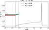 |
Fig. 5. Brunt-Väisälä frequency profile of two early models (Yc = 0.90) for 1 M⊙ with different values of the overshooting parameter, αov = 0.50 (blue) and αov = 0.15 (red). The vertical line indicates the fully mixed core boundary of each model. |
The result concerning the seismic parameters raises the question of a potential degeneracy between mass and overshooting (see Montalbán et al. 2013, for a detailed discussion of the degeneracy between period spacing and core overshooting during CHeB). Specifically, it suggests that the mass signature in the asymptotic period spacing can be replicated at fixed He-core mass by altering the extent of overshooting. We computed a model of 1 M⊙ with αov = 0.25, XCO = 5%, and 1.2 M⊙ with αov = 0.50, XCO = 5%. They exhibit this degeneracy where the track for one mass intersects that of another when the size of the overshooting region is adapted. For instance, the top panel of Fig. 6 illustrates that the track of the 1.2 M⊙ model with αov = 0.50 crosses the track of the 1 M⊙ model with αov = 0.25 several times, while their H-R diagram tracks are clearly distinct (bottom panel). This observation highlights the need for a more detailed analysis of such stars, as the ΔΠ − Δν diagram alone cannot reliably distinguish between mass and different mixing prescriptions because of this degeneracy. Given the valuable hidden information contained in transport processes such as convective overshooting, semi-convection, and potential rotational mixing at the border of the helium core, further investigation is required.
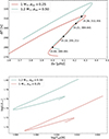 |
Fig. 6. Top panel: Asymptotic diagram Δν − ΔΠ of models 1.2 M⊙, αov = 0.50 and 1 M⊙, αov = 0.25. Markers indicate track crossings. Bottom panel: H-R diagram of corresponding models. |
4. Detailed analysis of the oscillation spectrum
In the previous section, we studied the potential impact of the internal structure and dynamics of a star on the global seismic parameters. In the following section, we analyse the oscillation spectra of our model grids at a specific stage of evolution on the horizontal branch to better grasp the impact of structural changes on the properties of individual oscillation modes. We begin with characterising their energy density to identify the effect on the seismic constraints related to the mixing zones near the core.
Using the eigenfunctions ξr and ξh, which respectively describe the radial and horizontal components of the displacement vector δr(r, θ, ϕ, t), we define the normalised inertia of a mode following Christensen-Dalsgaard (2004), as
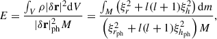 (4)
(4)
where the integration is over the volume of the star, and  is the squared norm of the displacement at the photosphere.
This approach allows us to identify the trapping properties of the modes and the parts of the star where the modes are confined, by analysing the variations in the energy density profile of the selected model alongside their seismic signatures in the spectrum. It is therefore helpful to characterise the regions contributing to mode trapping by extracting and analysing the specific modes exhibiting higher energies. This constitutes the first step in identifying relevant seismic features.
4.1. He-flash discontinuity
Core He-burning stars exhibit variations in their dynamics and structure depending on their evolutionary stage and the internal mixing processes acting in their core regions. For a solar mass CHeB star at an early stage Yc = 0.90, the internal structure is relatively simple, as the semi-convective layer has not yet appeared. We begin by examining the individual period-spacing ΔΠn, l of the computed l = 1 mode frequencies as a function of the frequency ν. A model without any “He-flash” signature (i.e. XCO = 0%) shows results similar to those of a typical shell hydrogen-burning RGB (Fig. 7 in red), where local minima correspond to modes trapped in the envelope and local maxima to modes trapped in the near-convective core regions, also called gravity-dominated mixed modes (Mosser et al. 2015). Since the chemical gradient ∇μ is responsible for mode trapping, it significantly impacts the seismic parameters (see Sect. 2 for a discussion), and the variation of overshooting in the model shows similar results to the global period spacing (see Sect. 3), where the spectrum of models with a larger overshooting zone is shifted towards higher asymptotic ΔΠ values.
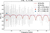 |
Fig. 7. Period spacing of computed ℓ = 1 mode frequencies for 1 M⊙, Yc = 0.90 models with differing carbon production from the He-flash. This figure compares models with XCO = 5% (grey dots) and XCO = 0% (red dots) along with the asymptotic value for the XCO = 0% model (solid violet line). |
As introduced earlier, the He-flash discontinuity at the end of the helium core corresponds to a sharp change in the chemical composition caused by the depletion of helium into carbon at the beginning of the core helium burning phase. This creates a sharp transition in the profile of N. By adding the sharp transition associated with the He-flash – where the parameter is denoted XCO = 5% – we observe a significant seismic impact. The expected location of this discontinuity, in terms of the normalised buoyancy radius (e.g. Miglio et al. 2008; Cunha et al. 2015; Bossini et al. 2015), is perfectly compatible with the periodicity of the glitch signature in the period spacing. The amplitude of this small discontinuity imparts its own signature and seems to act as an additional trapping cavity for the modes, as shown in the grey spectrum in Fig. 7, compared to the previous spectrum with XCO = 0% in red. Consequently, the model parameter associated with the He-flash – or any other mixing responsible for this sharp variation – seems relevant in the decomposition of the overall energy density profile.
The corresponding energy density profile associated with Fig. 7 displays two main characteristics. First, it exhibits a general pattern of local maxima and minima, typical of mixed modes and reminiscent of shell hydrogen-burning RGBs, where modes trapped in the deep g-mode cavity have higher inertia, and those trapped in the envelope p-mode cavity have lower inertia. Second, for the case of XCO = 5%, the profile features sawtooth patterns superimposed on the main trend. At low frequencies, the structure becomes even more complex, featuring a more intricate transition signature.
To analyse the origin of these sawtooth patterns, we examined the integrand of the energy density, defined in Eq. (4), for two successive sawtooth modes. The resulting profiles clearly indicate that the mode with a local maximum in energy is trapped within the intermediate radiative zone, which is characterised by the so-called He-flash discontinuity. We show an example of trapping in this specific zone for our 1 M⊙ and Yc = 0.90 model in Fig. 8, compared to the corresponding Brunt-Väisälä frequency profile. This figure presents two successive modes selected from the same 1 M⊙ model with Yc = 0.90 and XCO = 5%. These modes, also marked in blue and red in Fig. 7, are highlighted in the energy density profile of the same model (Fig. C.1) to illustrate that mode trapping is essentially a question of variations in mode inertia.
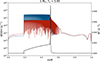 |
Fig. 8. Logarithmic-scale integrand of the energy density for two successive modes of the 1 M⊙, Yc = 0.90 model including the He-flash discontinuity, compared to the Brunt-Väisälä frequency profile (black line). Purple and green markers respectively indicate the sharp transitions of the Brunt-Väisälä frequency profile at the core and the He-flash discontinuity. |
The first marker on the Brunt-Väisälä frequency profile corresponds to the sharp boundary of the convective core, where the Brunt-Väisälä profile jumps due to the change to radiative stratification in the model. The second one is linked to the He-flash and hides a Dirac delta distribution in the Brunt-Väisälä frequency profile. The treatment of this discontinuity might not be fully representative of the actual signature of the evolution through the He-flash or the various associated “sub-flashes”; yet, it remains indicative of the impact on the seismic constraints by the sharp chemical gradients between the convective helium core and the hydrogen shell.
4.2. Transition sharpness
The sharp discontinuity included in CLES at one of the important transition zones in these stars, namely the helium flash discontinuity, is a prescription applied to simplify the initial conditions of this phase. However, as briefly mentioned above, this sharpness might not fully reflect the actual physical processes that occur in these stars. For example, the additional mixing of various physical origins (convective penetration, plumes, or rotational mixing) and forms (diffusive or convective) could be responsible for such signatures (Viallet et al. 2015). They could also smooth out – or even erase – the discontinuities potentially generated by sub-flashes over time, leading to more gradual transitions.
The question of how a smoother transition impacts the seismic properties of the star can be explored further, and to obtain a first look at how it could influence our seismic study, we implemented a post-treatment to our models to smooth out this transition. The discontinuous helium profile leads to a Brunt-Väisälä frequency, which exhibits a Dirac delta distribution at this location, since the Brunt-Väisälä frequency is directly linked to the density derivative (see Eq. 3). If we model the glitch in N using a Gaussian approximation, modifying the width and amplitude of the distribution changes the transition sharpness in the density profile. We do this within a defined radial interval Δr around the transition, where we apply the function  . Here a, b, and c2 denote the amplitude, position of the peak, and the variance, respectively. We applied this approach to the Brunt-Väisälä frequency (Eq. 3) and recalculated the other structural functions of interest (e.g. density, pressure, and Γ1) to obtain the theoretical spectrum of our smoothed models. We explored various width values for the parameter c, corresponding to different degrees of smoothing, ensuring that the density difference, denoted Δρ, in the region immediately before and after the transition remained constant by adjusting the amplitude a of the Gaussian function, accordingly.
Fig. 9 illustrates two examples of density sharp transition smoothing (smoothing A and B), derived from the corresponding Gaussian approximations of the Brunt–Väisälä frequency, alongside the resulting oscillation spectra before and after smoothing. As anticipated, a lower peak value in N2 leads to a smoother density transition. When extended to larger widths and lower amplitudes, the boundary is simply erased, eliminating mode trapping in this region (see Cunha et al. 2019, for details about Gaussian structural glitches). This explains why the spectrum reduces the amplitude of the additional peaks and reverts to the structure observed in Fig. 7 for the model XCO = 0%. In contrast, narrowing the peak to an extreme recreates a sharp boundary as the Gaussian converges to a Dirac delta distribution (Cunha et al. 2019). Another modification consists in altering the radial location of the transition to study its impact on the energy density profile and the modes spectrum. We modified our model by radially shifting the location of the transition, thereby reducing the size of the trapping zone between the boundary of the COS zone and the He-flash transition. This results in a decrease in the number of modes trapped inside this intermediate region. Given the precision of Kepler data, we expect to disentangle these various cases with high significance (see Mosser et al. 2024b, for a recent illustration). Finally, we also tested different resolutions to define the Gaussian function added to the Brunt-Väisälä profile to ensure that the main glitch signatures were not due to numerical issues.
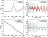 |
Fig. 9. Left panels: Density and Brunt-Väisälä frequency profiles of two smoothed 1 M⊙ models, A (Gaussian parameters: amplitude = 9e−10 s−2, width = 7e6 cm) and B (Gaussian parameters: amplitude = 6e−10 s−2, width = 2e7 cm) around the He-flash discontinuity, compared to the model with a sharp transition. Right panels: Period-spacing structure of mode frequencies for the smoothed models A and B (red dots), compared to the sharp transition model (grey dots). |
These comparisons show the sensitivity of asteroseismic constraints to the physical nature of the mixing processes acting in these regions, which may help calibrate in the future the prescriptions used in stellar evolution codes. As we demonstrated, a modification of the chemical gradient resulting from mixing processes, regardless of their origin, directly impacts the observed seismic signature displayed in the models and shows the diagnostic potential of detailed asteroseismic modelling of these stars.
4.3. Semi-convective zone
In our grid of models with an overshooting of αov = 0.50, the semi-convective layer emerges during an advanced evolutionary phase, around a central helium abundance of Yc ∼ 0.56. This is influenced by the convective overshooting implemented, where a different αov changes the Yc of the appearance of the semi-convective layer. The semi-convective layer, a region of partial mixing, affects both the chemical gradient and the Brunt-Väisälä frequency profiles, introducing distinct variations in the energy density profile. These signatures appear as sharp energy peaks detached from the main trend, producing a more complex oscillation spectrum, even in models where the He-flash discontinuity has been smoothed or removed. A detailed analysis of the energy density (Eq. 4) of the modes associated with these peaks reveals that they are confined within the semi-convective region, delimited by sharp variations in the Brunt-Väisälä frequency profile at the lower and upper boundaries of this zone, as illustrated in Fig. 10 for our model with Yc = 0.40. We recall that the internal structure and gradients of this model correspond to Fig. 4a in the simpler case with XCO = 0%. Another key observation comes from the associated spectrum in Fig. 11 in red. The local minima (red dots) correspond to the modes trapped in the semi-convective region, although most of these modes exhibit an exceptionally high energy density (Eq. 4), as shown in Fig. 12 with an order of magnitude 103 times higher.
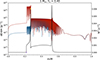 |
Fig. 10. Integrand of energy density in logarithmic scale of two successive modes for the 1 M⊙, Yc = 0.40 model, without He-flash discontinuity XCO = 0% and compared with the Brunt-Väisälä frequency profile (black line). Purple and yellow markers indicate the lower and upper semi-convective boundaries. |
 |
Fig. 11. Period spacing of computed ℓ = 1 mode frequencies, for 1 M⊙, Yc = 0.40 models with two different productions of carbon due to the He-flash, XCO = 5% (grey dots) and XCO = 0% (red dots), compared with the asymptotic value of the XCO = 0% model (solid violet line). |
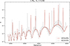 |
Fig. 12. Energy density of modes in 1 M⊙, Yc = 0.40 models for two sizes of He-flash discontinuity, corresponding to carbon production fractions of XCO = 5% (grey dots) and XCO = 0% (red dots). |
Their high energy density indicates that they are unlikely to be detected at the current level of data quality (see Grosjean et al. 2014 for a theoretical study of the detectability of the modes in RGBs). Removing them from the spectrum and computing again the difference in consecutive mode period shows little to no effect on the period spacing of the neighbouring modes. It suggests a strong decoupling between the cavities in the star, making it quite difficult to detect the influence of these modes, even indirectly through their interactions with their neighbours. This point is consistent with previous studies (Pinçon & Takata 2022), suggesting that larger and sharper transitions at the top of the semi-convective region enhance the decoupling between oscillation cavities.
In the grid of models studied, we explore the visibility of modes trapped in the semi-convective region by examining less evolved models, particularly those near the emergence of this region around Yc = 0.56. In these cases, one or two trapped modes do not exhibit such extreme jumps in their energies, possibly making them detectable in long-duration photometric observations. It is important to note that the visibility of these trapped modes could be influenced by other mixing prescriptions for the semi-convective zone or by varying mass regimes, presenting an interesting opportunity for further investigation. Indeed, hydrodynamical simulations currently predict diverse profiles, while we only tested here the classic induced semi-convection scheme used in other stellar evolution codes. Nevertheless, we show that, from a theoretical standpoint, mixed modes are strongly influenced by a semi-convective zone, the main issue being the detectability of the modes trapped in these very deep layers.
5. Conclusion
In this study, we examined the influence of internal mixing processes on seismic parameters of CHeB RGBs throughout their evolution sequence, focusing on how the helium-flash discontinuity, or other physical processes responsible for this transition, and the overshooting parameter impact mixed-modes oscillation spectra. As a first step towards further exploration of our models, we fixed the helium core mass mHe to 0.50 M⊙ to reduce analysis complexity and isolate the effects of other free parameters, such as the effect of the helium-flash remnants. We show that:
-
Sharp variations in chemical composition generate distinct mode-trapping effects, shaping the frequency structure and period-spacing patterns of oscillation modes.
-
Variations in overshooting influence the extent of the semi-convective region, modulating the Brunt–Väisälä frequency and the observed period spacing.
-
Adjustments in the overshooting parameter are compensated by changes in the relative size of the semi-convective layer, leading to a relatively constant COS zone size from the moment the semi-convective zone appears.
-
While the model evolution remains mostly unaffected, the seismic signature is highly sensitive to these internal changes because of their strong impact on the Brunt–Väisälä frequency profile, which directly affects the period spacing.
-
Detailed asteroseismic studies are essential for characterising mixing processes in the mixed core region of CHeB stars.
The seismic signatures notably seen in the Brunt–Väisälä frequency profile show the potential of asteroseismic observations for probing the dynamics of these regions. Constraining the mixing properties at the boundary of the helium core influence the amount of carbon and oxygen synthesised during CHeB. Moreover, mixing is shown to affect not only the properties of breathing pulses (Castellani et al. 1985) but also the duration of the asymptotic giant branch (AGB) phase and the properties of the AGB-bump (Bossini et al. 2015; Dréau et al. 2022). We refer to Matteuzzi et al. (2025) for a detailed description of the expected seismic signatures associated with different types of structural glitches in semi-analytical models of CHeB stars.
Recent 3D simulations (Blouin et al. 2024; Fuentes 2025) have provided additional perspectives on semi-convective mixing, with some studies emphasising the role of rotation in influencing semi-convective regions. These results suggest that rotational effects could be an important factor for exploration in future models.
Future work will expand on this framework by exploring various mixing prescriptions, as well as the treatment of mode coupling across multiple oscillation cavities (Pinçon & Takata 2022; Vrard et al. 2022; Mosser et al. 2024b). Starting from theoretical considerations and observations based on a consistent model with various mixing prescriptions, we will compare the observed seismic signatures to our theoretical predictions and aim at building a coherent picture of the oscillation spectrum of low-mass CHeB stars, similarly to the work by Farnir et al. (2021) for subgiants. Developing detailed seismic analysis techniques for CHeB stars will yield valuable seismic constraints on mixing processes acting in stellar interiors and allow for a deeper characterisation of their chemical properties throughout this evolutionary phase. Ultimately, the derivation of seismic indicators, complemented by their potential integration in detailed modelling strategies, contributes to the broader objective of understanding chemical and angular momentum transport processes in stellar interiors through asteroseismology. Further investigations will also be carried out using evolutionary models to calibrate more precisely the helium core mass parameter mHe, the XCO parameter, and the associated helium mass fraction profile between the convective core and the hydrogen shell.
TESS and Kepler have already observed more than 100 000 RGBs across the sky, including numerous CHeB stars, providing a rich dataset for seismic analysis. Additionally, the precise and accurate characterisation of CHeB stars is critical for Galactic archaeology, as it allows for the study of more evolved stellar populations and provides a better understanding of the properties of convective cores during this unique evolutionary phase, which strongly influences chemical yields at later stages (Herwig 2005). Applied in stellar clusters, a detailed characterisation of CHeB stars would also be key to quantify the properties of mass loss on the RGB (Howell et al. 2022, 2024, 2025; Tailo et al. 2022), while detailed studies of the coupling properties of mixed modes in this evolutionary stage might help characterise non-standard products of evolution (van Rossem et al. 2024). In this context, the future PLATO mission (Rauer et al. 2025) will play an important role for Galactic archaeology (Miglio et al. 2017), while other missions such as HAYDN (Miglio et al. 2021), will provide the necessary data to test the limitations of our models in single stellar populations. In this context, improving our asteroseismic analysis techniques is paramount to fully exploit the outputs of ongoing and future missions.
At higher masses, our input parameter representing the helium core mass must be adjusted in order for the models to remain consistent with the predictions of evolutionary computations.
Acknowledgments
We thank J. Montalbán for her contribution. L.P. is supported by the FNRS (“Fonds National de la Recherche Scientifique”) through a FRIA (“Fonds pour la Formation à la Recherche dans l’Industrie et l’Agriculture”) doctoral fellowship. G.B. acknowledges fundings from the Fonds National de la Recherche Scientifique (FNRS) as a postdoctoral researcher. M.M. and A.M. acknowledge support from the ERC Consolidator Grant funding scheme (project ASTEROCHRONOMETRY, https://www.asterochronometry.eu, G.A. n. 772293).
References
- Angulo, C., Arnould, M., Rayet, M., et al. 1999, Nucl. Phys. A, 656, 3 [Google Scholar]
- Asplund, M., Grevesse, N., Sauval, A. J., & Scott, P. 2009, Annu. Rev. Astron. Astrophys., 47, 481 [CrossRef] [Google Scholar]
- Auvergne, M., Bodin, P., Boisnard, L., et al. 2009, A&A, 506, 411 [NASA ADS] [CrossRef] [EDP Sciences] [Google Scholar]
- Bedding, T. R., Mosser, B., Huber, D., et al. 2011, Nature, 471, 608 [Google Scholar]
- Blouin, S., Herwig, F., Mao, H., Denissenkov, P., & Woodward, P. R. 2024, MNRAS, 527, 4847 [Google Scholar]
- Borucki, W. J., Koch, D., Basri, G., et al. 2010, Science, 327, 977 [Google Scholar]
- Bossini, D., Miglio, A., Salaris, M., et al. 2015, MNRAS, 453, 2290 [Google Scholar]
- Bressan, A., Marigo, P., Girardi, L., Nanni, A., & Rubele, S. 2013, Eur. Phys. J. Web Conf., 43, 03001 [Google Scholar]
- Castellani, V., & Tornambe, A. 1982, MNRAS, 198, 861 [Google Scholar]
- Castellani, V., Giannone, P., & Renzini, A. 1971a, Astrophys. Space Sci., 10, 355 [Google Scholar]
- Castellani, V., Giannone, P., & Renzini, A. 1971b, Ap&SS, 10, 340 [NASA ADS] [CrossRef] [Google Scholar]
- Castellani, V., Giannone, P., & Renzini, A. 1972, Ap&SS, 17, 80 [Google Scholar]
- Castellani, V., Chieffi, A., Tornambe, A., & Pulone, L. 1985, ApJ, 296, 204 [Google Scholar]
- Chaplin, W. J., & Miglio, A. 2013, ARA&A, 51, 353 [Google Scholar]
- Christensen-Dalsgaard, J. 2004, Sol. Phys., 220, 137 [Google Scholar]
- Claret, A., & Torres, G. 2016, A&A, 592, A15 [NASA ADS] [CrossRef] [EDP Sciences] [Google Scholar]
- Claret, A., & Torres, G. 2019, ApJ, 876, 134 [Google Scholar]
- Constantino, T., Campbell, S. W., Christensen-Dalsgaard, J., Lattanzio, J. C., & Stello, D. 2015, MNRAS, 452, 123 [Google Scholar]
- Cristini, A., Meakin, C., Hirschi, R., et al. 2016, Phys. Scr., 91, 034006 [Google Scholar]
- Cunha, M. S., Stello, D., Avelino, P. P., Christensen-Dalsgaard, J., & Townsend, R. H. D. 2015, ApJ, 805, 127 [NASA ADS] [CrossRef] [Google Scholar]
- Cunha, M. S., Avelino, P. P., Christensen-Dalsgaard, J., et al. 2019, MNRAS, 490, 909 [Google Scholar]
- Cunha, M. S., Damasceno, Y. C., Amaral, J., et al. 2024, A&A, 687, A100 [NASA ADS] [CrossRef] [EDP Sciences] [Google Scholar]
- Degl’Innocenti, S., Prada Moroni, P. G., Marconi, M., & Ruoppo, A. 2008, Ap&SS, 316, 25 [Google Scholar]
- Deheuvels, S., & Belkacem, K. 2018, A&A, 620, A43 [NASA ADS] [CrossRef] [EDP Sciences] [Google Scholar]
- Deheuvels, S., Doğan, G., Goupil, M. J., et al. 2014, A&A, 564, A27 [NASA ADS] [CrossRef] [EDP Sciences] [Google Scholar]
- Deheuvels, S., Ballot, J., Beck, P. G., et al. 2015, A&A, 580, A96 [NASA ADS] [CrossRef] [EDP Sciences] [Google Scholar]
- Deheuvels, S., Brandão, I., Silva Aguirre, V., et al. 2016, A&A, 589, A93 [NASA ADS] [CrossRef] [EDP Sciences] [Google Scholar]
- Dréau, G., Lebreton, Y., Mosser, B., Bossini, D., & Yu, J. 2022, A&A, 668, A115 [NASA ADS] [CrossRef] [EDP Sciences] [Google Scholar]
- Eggenberger, P., Montalbán, J., & Miglio, A. 2012, A&A, 544, L4 [NASA ADS] [CrossRef] [EDP Sciences] [Google Scholar]
- Farnir, M., Pinçon, C., Dupret, M.-A., Noels, A., & Scuflaire, R. 2021, A&A, 653, A126 [NASA ADS] [CrossRef] [EDP Sciences] [Google Scholar]
- Ferguson, J. W., Alexander, D. R., Allard, F., et al. 2005, ApJ, 623, 585 [Google Scholar]
- Fuentes, J. R. 2025, ArXiv e-prints [arXiv:2502.15111] [Google Scholar]
- Gabriel, M., Noels, A., Montalbán, J., & Miglio, A. 2014, A&A, 569, A63 [NASA ADS] [CrossRef] [EDP Sciences] [Google Scholar]
- Gehan, C., Mosser, B., Michel, E., Samadi, R., & Kallinger, T. 2018, A&A, 616, A24 [NASA ADS] [CrossRef] [EDP Sciences] [Google Scholar]
- Giammichele, N., Charpinet, S., Fontaine, G., et al. 2018, Nature, 554, 73 [NASA ADS] [CrossRef] [Google Scholar]
- Girardi, L. 2016, ARA&A, 54, 95 [Google Scholar]
- Grosjean, M., Dupret, M. A., Belkacem, K., et al. 2014, A&A, 572, A11 [CrossRef] [EDP Sciences] [Google Scholar]
- Hekker, S., & Christensen-Dalsgaard, J. 2017, A&ARv, 25, 1 [Google Scholar]
- Herwig, F. 2005, ARA&A, 43, 435 [NASA ADS] [CrossRef] [Google Scholar]
- Howell, M., Campbell, S. W., Stello, D., & De Silva, G. M. 2022, MNRAS, 515, 3184 [NASA ADS] [CrossRef] [Google Scholar]
- Howell, M., Campbell, S. W., Stello, D., & De Silva, G. M. 2024, MNRAS, 527, 7974 [Google Scholar]
- Howell, M., Campbell, S. W., Kalup, C., Stello, D., & De Silva, G. M. 2025, MNRAS, 536, 1389 [Google Scholar]
- Iglesias, C. A., & Rogers, F. J. 1996, ApJ, 464, 943 [NASA ADS] [CrossRef] [Google Scholar]
- Irwin, A. W. 2012, Astrophysics Source Code Library [record ascl:1211.002] [Google Scholar]
- Khan, S., Hall, O. J., Miglio, A., et al. 2018, ApJ, 859, 156 [NASA ADS] [CrossRef] [Google Scholar]
- Kippenhahn, R., & Weigert, A. 2013, Stellar Structure and Evolution (New York: Springer-Verlag) [Google Scholar]
- Kippenhahn, R., Weigert, A., & Weiss, A. 2012, Stellar Structure and Evolution, Astronomy and Astrophysics Library (Berlin Heidelberg: Springer) [Google Scholar]
- Kunz, R., Fey, M., Jaeger, M., et al. 2002, ApJ, 567, 643 [CrossRef] [Google Scholar]
- Lagarde, N., Charbonnel, C., Decressin, T., & Hagelberg, J. 2011, A&A, 536, A28 [NASA ADS] [CrossRef] [EDP Sciences] [Google Scholar]
- Lagarde, N., Decressin, T., Charbonnel, C., et al. 2012, A&A, 543, A108 [NASA ADS] [CrossRef] [EDP Sciences] [Google Scholar]
- Lindsay, C. J., Ong, J. M. J., & Basu, S. 2024, ApJ, 965, 171 [Google Scholar]
- Maeder, A. 1975, A&A, 43, 61 [NASA ADS] [Google Scholar]
- Marques, J. P., Goupil, M. J., Lebreton, Y., et al. 2013, A&A, 549, A74 [NASA ADS] [CrossRef] [EDP Sciences] [Google Scholar]
- Matteuzzi, M., Buldgen, G., Dupret, M.-A., et al. 2025, A&A, 700, A261 [NASA ADS] [CrossRef] [EDP Sciences] [Google Scholar]
- Miglio, A., Montalbán, J., Noels, A., & Eggenberger, P. 2008, MNRAS, 386, 1487 [Google Scholar]
- Miglio, A., Chiappini, C., Mosser, B., et al. 2017, Astron. Nachr., 338, 644 [Google Scholar]
- Miglio, A., Girardi, L., Grundahl, F., et al. 2021, Exp. Astron., 51, 963 [NASA ADS] [CrossRef] [Google Scholar]
- Mirouh, G. M., Garaud, P., Stellmach, S., Traxler, A. L., & Wood, T. S. 2012, ApJ, 750, 61 [NASA ADS] [CrossRef] [Google Scholar]
- Montalbán, J., Miglio, A., Noels, A., Scuflaire, R., & Ventura, P. 2010, ApJ, 721, L182 [Google Scholar]
- Montalbán, J., Miglio, A., Noels, A., et al. 2013, ApJ, 766, 118 [Google Scholar]
- Mosser, B., Belkacem, K., Goupil, M. J., et al. 2011, A&A, 525, L9 [CrossRef] [EDP Sciences] [Google Scholar]
- Mosser, B., Goupil, M. J., Belkacem, K., et al. 2012, A&A, 548, A10 [NASA ADS] [CrossRef] [EDP Sciences] [Google Scholar]
- Mosser, B., Michel, E., Belkacem, K., et al. 2013, A&A, 550, A126 [CrossRef] [EDP Sciences] [Google Scholar]
- Mosser, B., Vrard, M., Belkacem, K., Deheuvels, S., & Goupil, M. J. 2015, A&A, 584, A50 [NASA ADS] [CrossRef] [EDP Sciences] [Google Scholar]
- Mosser, B., Dréau, G., Pinçon, C., et al. 2024a, A&A, 681, L20 [NASA ADS] [CrossRef] [EDP Sciences] [Google Scholar]
- Mosser, B., Belkacem, K., Cunha, M. S., et al. 2024b, 8th TESS/15th Kepler Asteroseismic Science Consortium Workshop, 19 [Google Scholar]
- Moyano, F. D., Eggenberger, P., Meynet, G., et al. 2022, A&A, 663, A180 [NASA ADS] [CrossRef] [EDP Sciences] [Google Scholar]
- Moyano, F. D., Eggenberger, P., Mosser, B., & Spada, F. 2023, A&A, 673, A110 [NASA ADS] [CrossRef] [EDP Sciences] [Google Scholar]
- Noels, A. 2013, Lect. Notes Phys., 865, 209 [Google Scholar]
- Noll, A., & Deheuvels, S. 2023, A&A, 676, A70 [NASA ADS] [CrossRef] [EDP Sciences] [Google Scholar]
- Noll, A., Deheuvels, S., & Ballot, J. 2021, A&A, 647, A187 [EDP Sciences] [Google Scholar]
- Pinçon, C., & Takata, M. 2022, A&A, 661, A139 [NASA ADS] [CrossRef] [EDP Sciences] [Google Scholar]
- Pinçon, C., Goupil, M. J., & Belkacem, K. 2020, A&A, 634, A68 [Google Scholar]
- Rauer, H., Aerts, C., Cabrera, J., et al. 2025, Exp. Astron., 59, 26 [Google Scholar]
- Ricker, G. R., Winn, J. N., Vanderspek, R., et al. 2014, J. Astron. Telesc. Instrum. Syst., 1, 014003 [Google Scholar]
- Rizzuti, F., Hirschi, R., Georgy, C., et al. 2022, MNRAS, 515, 4013 [NASA ADS] [CrossRef] [Google Scholar]
- Salaris, M., & Cassisi, S. 2017, Roy. Soc. Open Sci., 4, 170192 [Google Scholar]
- Scuflaire, R., Théado, S., Montalbán, J., et al. 2008, Ap&SS, 316, 83 [Google Scholar]
- Serenelli, A., & Weiss, A. 2005, A&A, 442, 1041 [NASA ADS] [CrossRef] [EDP Sciences] [Google Scholar]
- Shibahashi, H. 1979, PASJ, 31, 87 [NASA ADS] [Google Scholar]
- Siess, L. 2009, A&A, 497, 463 [NASA ADS] [CrossRef] [EDP Sciences] [Google Scholar]
- Straniero, O., Dominguez, I., Imbriani, G., & Piersanti, L. 2003, ApJ, 583, 878 [NASA ADS] [CrossRef] [Google Scholar]
- Tailo, M., Corsaro, E., Miglio, A., et al. 2022, A&A, 662, L7 [NASA ADS] [CrossRef] [EDP Sciences] [Google Scholar]
- Takata, M. 2016, PASJ, 68, 109 [NASA ADS] [CrossRef] [Google Scholar]
- Tassoul, M. 1980, ApJS, 43, 469 [Google Scholar]
- van Rossem, W. E., Miglio, A., & Montalbán, J. 2024, A&A, 691, A177 [NASA ADS] [CrossRef] [EDP Sciences] [Google Scholar]
- Ventura, P., D’Antona, F., & Mazzitelli, I. 2008, Ap&SS, 316, 93 [CrossRef] [Google Scholar]
- Viallet, M., Meakin, C., Prat, V., & Arnett, D. 2015, A&A, 580, A61 [NASA ADS] [CrossRef] [EDP Sciences] [Google Scholar]
- Viani, L. S., & Basu, S. 2020, ApJ, 904, 22 [NASA ADS] [CrossRef] [Google Scholar]
- Vrard, M., Cunha, M. S., Bossini, D., et al. 2022, Nat. Commun., 13, 7553 [CrossRef] [Google Scholar]
- Weiss, A., Hillebrandt, W., Thomas, H.-C., & Ritter, H. 2004, Cox and Giuli’s Principles of Stellar Structure (Cambridge: Cambridge Scientific Publishers) [Google Scholar]
- Wood, T. S., Garaud, P., & Stellmach, S. 2013, ApJ, 768, 157 [NASA ADS] [CrossRef] [Google Scholar]
- Zahn, J. P. 1991, A&A, 252, 179 [Google Scholar]
Appendix A: Effect of overshooting on oscillation spectrum
As illustrated in Fig. A.1, the individual period-spacing is influenced by the overshooting length put in the model. A model with a lower αov has a smaller fully mixed core and the integral of the Brunt-Väisälä frequency in the semi-convective layer is higher. This explains the lower asymptotic period-spacing in this case.
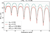 |
Fig. A.1. Period spacing of computed ℓ = 1 mode frequencies, for 1 M⊙, Yc = 0.90 models, with two different values of the overshooting parameter, αov = 0.50 (blue dots) and αov = 0.15 (red dots), compared with their asymptotic value ΔΠ (dashed lines). |
Appendix B: Kippenhahn diagrams
We show Kippenhahn diagrams (Fig. B.1) to illustrate the internal mixing processes during the core helium-burning phase of our models. Specifically, we present the models 1M⊙ with αov = 0.50 and 0.15. These diagrams provide a representation of the evolution of the convective core, overshooting, and semi-convective regions within the star.
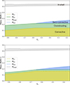 |
Fig. B.1. Top panel: Kippenhahn diagram showing the structural evolution of the 1M⊙ model with αov = 0.50, featuring the convective core, overshooting zone, semi-convective zone, and hydrogen-burning shell. Bottom panel: Kippenhahn diagram showing the structural evolution of the 1M⊙ model with αov = 0.15. |
Appendix C: Energy density profile of an early model
The energy density profile for a 1M⊙ model with Yc = 0.90 is shown for two cases: XCO 0% and XCO = 5%. The profiles display a sawtooth pattern corresponding to mode trapping caused by the discontinuity left by the helium flash, as illustrated in Fig. C.1. The blue and red markers indicate two selected modes, one of which is trapped in the cavity formed by this discontinuity.
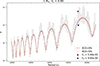 |
Fig. C.1. Energy density of the modes of 1 M⊙, Yc = 0.90 models for two sizes of the He-flash discontinuity (implying changes in the density jump at this location) corresponding to carbon production fractions of XCO = 5% (grey dots) and XCO = 0% (red dots). The red and blue markers indicate two selected modes. |
All Figures
|
Fig. 1. Gradient profile as a function of mass fraction for a one-solar-mass CHeB star at solar metallicity and Yc = 0.90. The helium profile is shown in parallel (black). The convective zone is in yellow; the overshooting layer is in green; and the sharp variation left by the “He flash” is in grey with XCO = 5%. The radiative gradient ∇rad is in red, and the adiabatic gradient ∇ad in blue. The real gradient ∇ is defined as follows: ∇ = ∇ad in the COS zone, and ∇ = ∇rad in the radiative zone. We focus on the central part of the star for illustrative purposes. |
| In the text | |
|
Fig. 2. Top panel: Evolutionary track in the Hertzsprung–Russell diagram of the sequence of models from 1 M⊙ to 1.5 M⊙ stellar masses at fixed He-core mass. The markers indicate the state of central helium abundance studied: Yc = 0.90, Yc = 0.40, and Yc = 0.10. Bottom panel: Central temperature as a function of the central density in logarithmic scale for the corresponding set of masses. |
| In the text | |
|
Fig. 3. Top panel: Diagram Δν − ΔΠ of three models of different stellar mass. Each point corresponds to a stage (Yc) in the evolution on the horizontal branch. The markers indicate the state of central helium abundance (Yc = 0.90, Yc = 0.40, and Yc = 0.10) and the appearance of the semi-convective layer. Bottom panel: Diagram Δν − ΔΠ of two models with different overshooting parameters αov. |
| In the text | |
|
Fig. 4. Comparison of overshooting parameters αov = 0.50 (top panel) and αov = 0.15 (bottom panel) for 1 M⊙ through the gradient and helium profiles as a function of the mass fraction at the same age, compared to the helium profile (black). The convective zone is in yellow; the overshooting layer is in green; the semi-convective zone is in blue; and the sharp variation left by the He-flash is in grey. The radiative gradient ∇rad is in red, and the adiabatic gradient ∇ad is in blue. The real gradient ∇ is defined as follows: ∇ = ∇ad in the COS zone, and ∇ = ∇rad in the radiative zone. |
| In the text | |
|
Fig. 5. Brunt-Väisälä frequency profile of two early models (Yc = 0.90) for 1 M⊙ with different values of the overshooting parameter, αov = 0.50 (blue) and αov = 0.15 (red). The vertical line indicates the fully mixed core boundary of each model. |
| In the text | |
|
Fig. 6. Top panel: Asymptotic diagram Δν − ΔΠ of models 1.2 M⊙, αov = 0.50 and 1 M⊙, αov = 0.25. Markers indicate track crossings. Bottom panel: H-R diagram of corresponding models. |
| In the text | |
|
Fig. 7. Period spacing of computed ℓ = 1 mode frequencies for 1 M⊙, Yc = 0.90 models with differing carbon production from the He-flash. This figure compares models with XCO = 5% (grey dots) and XCO = 0% (red dots) along with the asymptotic value for the XCO = 0% model (solid violet line). |
| In the text | |
|
Fig. 8. Logarithmic-scale integrand of the energy density for two successive modes of the 1 M⊙, Yc = 0.90 model including the He-flash discontinuity, compared to the Brunt-Väisälä frequency profile (black line). Purple and green markers respectively indicate the sharp transitions of the Brunt-Väisälä frequency profile at the core and the He-flash discontinuity. |
| In the text | |
|
Fig. 9. Left panels: Density and Brunt-Väisälä frequency profiles of two smoothed 1 M⊙ models, A (Gaussian parameters: amplitude = 9e−10 s−2, width = 7e6 cm) and B (Gaussian parameters: amplitude = 6e−10 s−2, width = 2e7 cm) around the He-flash discontinuity, compared to the model with a sharp transition. Right panels: Period-spacing structure of mode frequencies for the smoothed models A and B (red dots), compared to the sharp transition model (grey dots). |
| In the text | |
|
Fig. 10. Integrand of energy density in logarithmic scale of two successive modes for the 1 M⊙, Yc = 0.40 model, without He-flash discontinuity XCO = 0% and compared with the Brunt-Väisälä frequency profile (black line). Purple and yellow markers indicate the lower and upper semi-convective boundaries. |
| In the text | |
|
Fig. 11. Period spacing of computed ℓ = 1 mode frequencies, for 1 M⊙, Yc = 0.40 models with two different productions of carbon due to the He-flash, XCO = 5% (grey dots) and XCO = 0% (red dots), compared with the asymptotic value of the XCO = 0% model (solid violet line). |
| In the text | |
|
Fig. 12. Energy density of modes in 1 M⊙, Yc = 0.40 models for two sizes of He-flash discontinuity, corresponding to carbon production fractions of XCO = 5% (grey dots) and XCO = 0% (red dots). |
| In the text | |
|
Fig. A.1. Period spacing of computed ℓ = 1 mode frequencies, for 1 M⊙, Yc = 0.90 models, with two different values of the overshooting parameter, αov = 0.50 (blue dots) and αov = 0.15 (red dots), compared with their asymptotic value ΔΠ (dashed lines). |
| In the text | |
|
Fig. B.1. Top panel: Kippenhahn diagram showing the structural evolution of the 1M⊙ model with αov = 0.50, featuring the convective core, overshooting zone, semi-convective zone, and hydrogen-burning shell. Bottom panel: Kippenhahn diagram showing the structural evolution of the 1M⊙ model with αov = 0.15. |
| In the text | |
|
Fig. C.1. Energy density of the modes of 1 M⊙, Yc = 0.90 models for two sizes of the He-flash discontinuity (implying changes in the density jump at this location) corresponding to carbon production fractions of XCO = 5% (grey dots) and XCO = 0% (red dots). The red and blue markers indicate two selected modes. |
| In the text | |
Current usage metrics show cumulative count of Article Views (full-text article views including HTML views, PDF and ePub downloads, according to the available data) and Abstracts Views on Vision4Press platform.
Data correspond to usage on the plateform after 2015. The current usage metrics is available 48-96 hours after online publication and is updated daily on week days.
Initial download of the metrics may take a while.