| Issue |
A&A
Volume 704, December 2025
|
|
|---|---|---|
| Article Number | A6 | |
| Number of page(s) | 15 | |
| Section | Stellar structure and evolution | |
| DOI | https://doi.org/10.1051/0004-6361/202555600 | |
| Published online | 26 November 2025 | |
Calibration of binary population synthesis models using white dwarf binaries from APOGEE, GALEX, and Gaia
1
Max-Planck-Institut für Astrophysik, Karl-Schwarzschild-Str. 1, 85748 Garching b. München, Germany
2
Instituto de Astronomia, Geofísica e Ciências Atmosféricas, Universidade de São Paulo, Rua do Matão 1226, Cidade Universitária, 05508-900 São Paulo, SP, Brazil
3
Department of Physics, McWilliams Center for Cosmology and Astrophysics, Carnegie Mellon University, 5000 Forbes Avenue, Pittsburgh, PA 15213, USA
4
Department of Physics and Astronomy and Pittsburgh Particle Physics, Astrophysics and Cosmology Center (PITT PACC), University of Pittsburgh, 3941 O’Hara Street, Pittsburgh, PA 15260, USA
5
Department of Astronomy, California Institute of Technology, 1200 E. California Blvd., Pasadena, CA 91125, USA
6
Centro de Estudios de Física del Cosmos de Aragón (CEFCA), Plaza San Juan 1, 44001 Teruel, Spain
7
Department of Astronomy, University of Virginia, Charlottesville, VA 22904, USA
8
University of Wisconsin-Madison, 2535 Sterling Hall 475 N. Charter Street Madison, WI 53706, USA
9
Department of Physics and Astronomy, Vanderbilt University, Nashville, TN 37235, USA
10
Department of Physics, Fisk University, Nashville, TN 37208, USA
⋆ Corresponding author: This email address is being protected from spambots. You need JavaScript enabled to view it.
, This email address is being protected from spambots. You need JavaScript enabled to view it.
Received:
20
May
2025
Accepted:
18
September
2025
Abstract
The effectiveness and stability of mass transfer in a binary system are crucial for determining the final product of its evolution. Rapid binary population synthesis codes simplify the complex physics of mass transfer and common-envelope evolution by adopting parameterized prescriptions for the stability of mass transfer, accretion efficiency in stable mass transfer, and the efficiency of common-envelope ejection. Our goal is to calibrate these uncertain parameters by comparing binary population synthesis models with observational data. Binary systems composed of a white dwarf and main-sequence star are ideal for studying the effects of binary interaction, as they can be formed through stable or unstable mass transfer, or without any interaction. These different evolutionary paths affect the orbital period and masses of the present-day population. The APOGEE-GALEX-Gaia catalog (AGGC) provides a homogeneous sample of over 500 systems with well-measured radial velocities that can be used as a comparison baseline for population synthesis simulations of white dwarf–main-sequence binaries. We compare the distribution of the observed maximum radial velocity variation (ΔRVmax) in the AGGC to binary population models simulated with COSMIC, a publicly developed binary population synthesis code. Within these synthetic populations, we vary the mass transfer and common-envelope ejection efficiency, and the criteria for mass transfer stability at the first ascent, asymptotic, and thermally pulsing giant branch phases. We also compare our models to systems with orbital solutions and estimated stellar masses. The ΔRVmax comparison shows clear preference for models with a higher fraction of stars undergoing stable mass transfer during the first ascent giant branch phase, and for highly effective envelope ejection during common-envelope phases. For the few systems with estimated WD masses, a comparison to models shows a slight preference for nonconservative stable mass transfer. In COSMIC and similar codes, the envelope ejection efficiency and the envelope binding energy are degenerate parameters. Therefore, our result of a high ejection efficiency may indicate either that additional sources of energy (such as recombination energy from the expansion of the envelope) are required to eject the envelope, or that its binding energy is lower than traditionally assumed. Future comparisons to population synthesis simulations of WD binaries can be drawn for other datasets as they become available, such as upcoming Gaia data releases and the future LISA mission, and for binary systems in other evolutionary stages.
Key words: binaries : close / binaries: general / binaries: spectroscopic / white dwarfs
© The Authors 2025
 Open Access article, published by EDP Sciences, under the terms of the Creative Commons Attribution License (https://creativecommons.org/licenses/by/4.0), which permits unrestricted use, distribution, and reproduction in any medium, provided the original work is properly cited.
This article is published in open access under the Subscribe to Open model.
Open Access funding provided by Max Planck Society.
1. Introduction
White dwarfs (WDs) are the final stage of evolution for the majority of stars. While they are a straightforward end point for stars with masses below the threshold for central oxygen ignition (∼8 M⊙), WDs can also be formed via binary evolution and even be the result of mergers (Althaus et al. 2010). A binary system containing a WD can be formed through many different channels. Two stars can be born in a binary system but separate enough to never interact. As they evolve as single stars, the result can be a WD and a main sequence (MS), a giant, or another WD, depending mostly on their initial mass ratio and the age of the system. If the two stars are born close enough to interact, a WD can also be formed after a period of mass transfer, which can be stable or unstable. During mass transfer, the WD progenitor increases its radius and fills its Roche lobe. Depending on the stage of evolution of the two stars, their separation, and their mass ratio, this mass transfer can become unstable, leading to common envelope evolution (CEE), also resulting in a WD binary with closer orbital separations when compared to stable mass transfer (Ivanova et al. 2013; Toonen et al. 2017).
Regardless of the evolutionary path taken by each WD binary, the physical processes that mediate their formation should leave an imprint on the properties of the final population, such as their period and mass distributions. Thus, studies of large samples of WD binaries can provide information on binary stellar evolution, and in particular the still poorly understood CEE (e.g.,Zorotovic et al. 2010, 2011; De Marco et al. 2011; Postnov & Yungelson 2014; Scherbak & Fuller 2023). The two vital ingredients for this type of study are data and models that can be readily compared to each other, so that the stability and efficiency of mass transfer can be constrained. For instance, Zorotovic et al. (2010) used a sample of WD+MS binaries from SDSS to estimate the common envelope ejection efficiency, α, finding values in the range of 0.2 − 0.3 to represent the final parameters of most of their sample. The recent work of Scherbak & Fuller (2023) models the CEE of ten double WD binary systems using stellar evolution code MESA, finding a similar range for α, 0.2 − 0.4.
To understand the behavior of an entire population, however, the sample size of the data and the models must be large enough to be statistically relevant. The great multi-epoch surveys of the past decade have finally provided the community with larger, less biased datasets; combining such surveys allows for the assembly of curated catalogs of populations such as WD binaries. The recent APOGEE-Galex-Gaia catalog (AGGC – Anguiano et al. 2022) is one such effort to minimize biases, providing a sample of WD binaries selected with homogeneous, and relatively simple, criteria. On the modeling side, rapid binary population synthesis (BPS) codes, such as the BSE code from Hurley et al. (2002), can simulate large populations in a time- and resource-efficient fashion when compared to detailed stellar evolution modeling. These BPS codes use parametrized prescriptions for binary interactions at each step of the evolution of the system, following it from the zero-age MS to the final product. Thus, with observational and simulated populations in hand, the theoretical predictions can be compared to data, informing these widely used prescriptions and providing a better understanding of binary evolution.
In this work, we calibrate the mass transfer parameters in the BPS code COSMIC (Breivik et al. 2020) using a sample of WD+MS binaries from AGGC (Anguiano et al. 2022). In our COSMIC models, we explore different assumptions for the criteria for the onset of unstable mass transfer, limits on the accretion between stars during stable Roche-lobe overflow (RLOF), and the efficiency of envelope ejection in CEE. These models are compared to the WD+MS systems in the AGGC by their radial velocity shifts, orbital parameters, and stellar mass. Our results provide new estimates on the mass transfer parameters for WD+MS binaries, and are also applicable to other BPS codes that rely on the formalism of Hurley et al. (2002).
The rest of the paper is structured as follows. Section 2 describes the data contained in the AGGC, while Section 3 describes our BPS methodology. We discuss our results in Section 4 and compare them to previous work in Section 5. We finish with our conclusions in Section 6.
2. APOGEE-Gaia-Galex catalog (AGGC)
The catalog was compiled by (Anguiano et al. 2022) using near-infrared data from the 17th Data Release of the Apache Point Observatory Galactic Evolution Experiment (APOGEE data release 17) (Majewski et al. 2017; Abdurro’uf et al. 2022), ultraviolet (UV) data from GALEX (Bianchi et al. 2017), and optical data from the Gaia mission (Lindegren et al. 2021). With this combination, Anguiano et al. (2022) was able to identify WDs in systems with primary stars in a broad range of luminosities, from low-mass MS stars to giants. The APOGEE-Gaia-Galex catalog (AGGC) was compiled by cross-matching all the targets in APOGEE for which the APOGEE Stellar Parameters and Chemical Abundances Pipeline yielded valid atmospheric measurements with the GALEX (Bianchi et al. 2017) and WISE (Wright et al. 2010) databases. A full spectral energy distribution (SED) was derived for all the entries that had complete photometric information: two GALEX bands in the UV, four WISE bands in the mid infrared, plus the three Gaia bands in the optical and the three 2MASS bands in the near-infrared that are already part of the APOGEE database. Binary WD candidates were drawn from this sample by requiring an APOGEE Teff < 6000 K and a GALEX far-UV - near-UV measure of (FUV–NUV)° < 5. This cut is made to avoid contaminating the sample with RV variability that is due to pulsations rather than binary motion.
The contamination of the sample of WD binary candidates was reduced by removing known intruders (pulsating stars and variable stars) and performing two-component fits to the broadband SEDs, with a “cold” component fixed to a Kurucz model (Kurucz 1979) with the APOGEE stellar parameters (Teff, [M/H], and log g), and a “hot” component drawn from the Koester grid of atmospheric WD models (Koester 2010). The final sample of WD binary candidates in the AGGC was drawn by requiring that the equivalent radius of the WD, RWD, inferred from the SED fit be < 25R⊕. Below the limit of 5 R⊙ for the radius of the nondegenerate companion, the maximum RWD decreases following a slope of 0.7 + 6R of the nondegenerate stars (see the red lines in Figure 10 of Anguiano et al. 2022). In the upper left panel of Figure 1 we show the observational Hertzsprung-Russell diagram for the entire APOGEE sample in blue, with the 588 WD+MS binaries in the AGGC highlighted in orange. The black line defines our applied surface gravity cutoff for the MS companions (log g < 4). Figure 1 provides an overview of the observational data we use in this study, the candidate WD+MS binaries contained in the catalog.
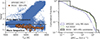 |
Fig. 1. Overview of the WD binaries in the APOGEE-Gaia-Galex catalog (AGGC). The left panel shows the full APOGEE dataset in blue and the companions of WDs in orange. The right panel shows the ΔRVmax distribution for different cuts in the data: MS+MS binaries from the full APOGEE dataset in blue, all WD binaries in the AGGC in green, and WD+MS binaries in black. The full APOGEE dataset contains 455796 targets; the MS binaries in that sample number 151266. The full AGGC has 1157 candidate WD binaries, while the WD+MS systems number 588. |
One key advantage of the AGGC is that the APOGEE data provides precise, multi-epoch radial velocities (ΔRV≈ 100 m s−1) for all objects in the sample. In most cases, the number of epochs available is not sufficient to derive a full orbital solution, but the maximum value of the RV variation (maximum minus minimum RV for each target), ΔRVmax, is a proxy for the orbital period, especially for ΔRVmax ≳ 10 km/s — see Badenes et al. (2018), Mazzola et al. (2020), and Anguiano et al. (2022) for discussions. These ΔRVmax measurements are an excellent figure of merit to single out short period binaries, as even accounting for random inclinations on the plane of the sky the highest ΔRVmax values will always be associated with the shortest orbital periods, and vice versa. Thus, statistically, ΔRVmax provides a noisy, but unbiased estimate for the orbital period distribution of a large population of binaries. In the right panel of Figure 1, we compare ΔRVmax values for all MS stars in APOGEE (dashed blue lines), the full AGGC sample (dotted green lines), and the WD+MS population in the AGGC (solid black lines). There is a stark difference in the shape of the cumulative distribution of ΔRVmax between the AGGC WD+MS binaries and the full APOGEE dataset. The fact that the AGGC WD+MS binaries have a ΔRVmax distribution skewed toward higher values indicates that the binaries in this sample have shorter periods than those of the APOGEE targets that show no evidence of a WD companion.
In addition to ΔRVmax, some systems in AGGC also have orbital information that we use in our analysis. Eleven WD+MS systems in AGGC have an orbital solution from Gaia data release 3, either from astrometry or from radial velocities (see Table 1). For the single-lined spectroscopic binaries (SB1), measurements of the semi-amplitude of the primary RV (K) are also available. These measurements can be combined with primary mass (MMS) estimates from the Bayesian isochrone-fitting code StarHorse (Queiroz et al. 2023) (also in Table 1) to estimate the minimum mass of the WD. For systems with only an astrometric solution, we can estimate K and consequently MWD using the Gaia estimates for the geometric Thiele-Innes elements (which relate to the classical elliptical orbital elements – see Appendix A of Halbwachs et al. 2023). The error on MWD is estimated using Monte Carlo (MC) error propagation. We also include two systems for which orbital parameters could be derived from their APOGEE RV curves (Corcoran et al. 2021).
Orbital parameters for AGGC systems with orbital solutions.
3. Binary population synthesis with COSMIC
Binary population synthesis codes are widely used in the study of populations of binary stars. The BPS calculations rely on tunable prescriptions to describe how the binary components and the orbit itself react to interactions via tides, wind mass loss, or RLOF, which can remain stable on radiative or thermal timescales or lead to dynamically unstable CEE. “Rapid" BPS codes implement single star evolution based on a grid of single star models computed by Pols et al. (1998) through a series of analytic formulae that are fit to the models (the “Hurley fits” —Hurley et al. 2000).
In this work, we use COSMIC1, a Python-based, open-developed BPS code that has been modified to incorporate several updates to binary interactions and contains modules for the creation and analysis of large binary populations (Breivik et al. 2020). While COSMIC has several parameters that control the evolution of binaries of all mass ranges, our main interest in this work are WD+MS binary systems. We explore three key binary evolution parameters in our COSMIC simulations, and otherwise apply the default assumptions as described in COSMIC v3.4.10:
-
β, which sets the fraction of the mass transferred from the donor that is accreted by the companion, with the rest being lost from the binary system (β = 0.5 assumes 50% accretion efficiency – Belczynski et al. 2008). It regulates the amount of mass accreted during stable RLOF and thus affects the masses of the MS stars in our simulated WD+MS binaries. Material that is not accreted is isotropically re-emitted from the vicinity of the accretor. Values range from 0 to 1.
-
α, the common envelope efficiency parameter, which scales the efficiency of transferring orbital energy to the envelope to eject it, as Ebind, i = α(Eorb, f − Eorb, i), (Eq. 71 of Hurley et al. 2002). α = 1 indicates that all of the change in orbital energy of the system was used to unbind the envelope; larger values imply that, in addition to the change in orbital energy, energy from another, unspecified source (e.g., recombination energy) was used.
-
qset, which selects the prescription used to determine critical mass ratios (qcrit, the ratio of donor mass/accretor mass) for the onset of unstable mass transfer and/or a common envelope during RLOF depending on the evolutionary state of the donor. The prescriptions we use are described in Table 2.
WD+MS systems can form via multiple evolutionary channels. Figure 2 illustrates these different evolutionary pathways. In our models, wide WD+MS systems can be formed without binary interactions, but the formation of close WD+MS binaries requires RLOF interactions to shrink the orbit. Systems that become WD+MS binaries with periods lower than ∼1000 days were likely subject to a mass transfer episode in their lifetime. A given binary will traverse a single path based on the chosen binary evolution model and initial binary properties, but large simulated populations allow us to map the most common pathways that are taken for different parts of the initial binary population under a given set of assumptions that make up our binary evolution model. Changing the binary evolution assumptions within COSMIC changes the recipes for the interactions that these systems go through, significantly modifying both specific evolutionary paths and the characteristics of the final simulated WD+MS population.
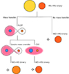 |
Fig. 2. Schematic of the possible evolutionary paths through which a binary system can go to become a WD+MS binary. The system can either not interact, or go through RLOF mass transfer, which can in turn be stable or unstable, leading to a common envelope phase. The imprints of their evolution can be seen in the final masses and orbital period of the systems. |
Whether a system goes through only stable mass transfer or through a phase of unstable mass transfer (such as CEE) depends not only on the initial separation of the system, but also on the amount of mass accreted during RLOF (β), the response of the orbit to the mass transfer, and the critical value for the mass ratio between the donor star and the accretor (qcrit). This critical value in turn depends on the evolutionary state of the donor at RLOF. We explore different values for qcrit for key evolutionary states, namely the first ascent, asymptotic, and thermally pulsing giant branch stages. We define the qset parameter to indicate which prescription a given model uses for its qcrit values. In COSMIC, there are different prescriptions for qcrit across the evolution of the star, as detailed in Table 2. The qset = 1 prescription follows Claeys et al. (2014), where Eq. 1 is
![Mathematical equation: $$ \begin{aligned} q_{\rm crit} = 2.13 \times \left[ 1.67 - x + 2\left( \frac{M_{c1}}{M_{1}}\right)^5\right]^{-1} , \end{aligned} $$](/articles/aa/full_html/2025/12/aa55600-25/aa55600-25-eq1.gif) (1)
(1)
with x ≈ 0.3 at solar metallicity (Hurley et al. 2002). The other prescriptions are the same, but vary the qcrit of key evolutionary states: qset = 2 has qcrit = 2.0 for asymptotic giant branch (AGB) stars, qset = 3 has qcrit = 2.0 for first ascent giant branch (FGB) stars, and qset = 4 has qcrit = 2.0 for thermally pulsing giant branch (TAGB) stars. For qset = 5, all giant stars (FGB, AGB and TAGB) have qcrit = 2.0. This setting makes RLOF initiated by these giant stars tend more toward stable mass transfer than CEE; the specific value of qcrit = 2.0 was chosen because it is a middle ground between the value used in the prescriptions of Hurley et al. (2002) and Belczynski et al. (2008).
If CEE happens, the fate of the system depends on the efficiency of the ejection of the envelope (α). COSMIC uses the αλ prescription of Hurley et al. (2002), where λ represents how bound the envelope is to its stellar core. Ebind is inversely proportional to λ, such that large values imply a less bound envelope. This parameter is calculated at each evolutionary state, following the description in Appendix A of Claeys et al. (2014). We do not explore different prescriptions for λ directly since the fits provided in Claeys et al. (2014) are drawn from the same stellar evolution models as the Hurley fits. Finally, we assume that the calculation of λ does not include recombination energy. However, α and λ are degenerate, and thus our parameter α can be interpreted as a conjugate parameter αλ. If ejection is very effective (α≥ 1), the system has higher chances of surviving without merging, forming binaries with wider orbital periods than compared to less effective ejection (α ≤ 1). The effects of α increasing or decreasing, however, could also be interpreted as increases or decreases in λ such that the envelope of a CEE donor is less or more bound to the core, respectively. In this work, we chose to vary α uniformly rather than explore various evolutionary state dependent prescriptions for λ.
We simulated several populations, each initialized with 5 × 10⁶ binary systems. These populations were initialized with primary masses drawn from the initial mass function from Kroupa (2001) between 0.08 and 150 M⊙, secondary masses drawn from a uniform distribution between M2 = 0.08 M⊙ and the primary mass, a uniform eccentricity distribution, and the period distribution from Raghavan et al. (2010). The populations all have solar metallicity and a uniform star formation history over the last 10 Gyr. Thiele et al. (2023) find that using a metallicity-dependent initial binary fraction in COSMIC can have a considerable effect on the size of the final population of WD binaries (in particular double WD systems). While this effect can be significant, we do not explore metallicity in this work since the impact of different assumptions for mass transfer far outweigh the incorporation of metallicity-specific close binary fractions.
We created 25 models varying α, β, and qset parameters according to Table 3. The models can be separated into three categories: low, middle, and high α. Models A and B have α = 0.3 and β = 0.0 and 1.0, respectively; model C has α = 1.0 and β = 1.0 (commonly assumed in population synthesis studies); and models D and E have α = 5.0 and β = 0.0 and 1.0, respectively. Within each family (A, B, C, D, and E), we also explored the five prescriptions of qset, labeled 1–5 for reference (see Table 2).
Values for qcrit used in the simulations.
Model names and parameters.
Table A.1 presents an overview of the number of systems in our simulations that end up as WD+MS binaries, double WDs (DWDs), and WD+non-MS stars; the remaining systems do not form a WD within the evolution time of the simulation (e.g., MS+MS), or merge before doing so. In this work, we focus only on the WD+MS population.
The result of each simulation, given our constant star formation history, is a “present-day” population of binaries, from which we gathered the WD+MS pairs and applied observational selection cuts to produce a synthetic catalog of WD+MS systems. As the AGGC has a UV magnitude cut, we imposed the same cut on our simulated populations We used the temperature of the two stars to estimate their combined black body emission in the far- and near-UV (FUV and NUV filters from GALEX) and removed systems with (FUV–NUV) < 5 from our synthetic catalogs (Anguiano et al. 2022). We also removed systems that are WD+MS binaries, but that are currently still interacting, as such systems are not expected to be present in the AGGC. Table A.1 shows the number of systems present in each COSMIC model before and after these criteria are imposed on the population.
The WD+MS sample of AGGC might be subject to contamination by nonbinary MS stars with strong chromospheric activity in the UV, particularly in the range (FUV–NUV) < 2. However, as the effects of chromospheric activity in the AGGC are not fully characterized, we do not include this magnitude cut in our modeling. There is also bias in both APOGEE and Gaia toward brighter MS targets; however, correcting our models for this bias is nontrivial and beyond the scope of our analysis since it would require assigning positions in the Galaxy and associated extinction and crowding. This choice leads to the inclusion of potential both lower- and higher-mass MS companions, where lower-mass companions may not be bright enough for APOGEE or Gaia to see, while higher-mass companions may be rarer and thus not present in the data. We discuss the impact of this choice below in Section 5.
To compare the COSMIC models directly to the AGGC data, we calculated the ΔRVmax distributions for each simulated population. The periods, mass ratios, and eccentricities of the binaries in each COSMIC model were used as the input to a MC code (Badenes et al. 2018; Mazzola et al. 2020) that generates random inclinations (in cosine space) and arguments of pericenter to project RV curves on the plane of the sky. From these RV curves, the MC code draws a random initial phase and samples RV values for a given number of epochs and distribution of cadences (i.e., the times at which these RV “measurements” were taken for each system). We used the cadence distribution from APOGEE data release 17 to accurately reflect the cadence in our simulated populations. Finally, the ΔRVmax was calculated for each sparsely sampled RV curve, resulting in a distribution of ΔRVmax for the synthetic catalog. As this is an MC code, the ΔRVmax distribution can be sampled many times, i.e., many sets of RVs can be obtained for the same system, given its inclination, argument of pericenter and time lag change at each realization. Thus, we can also estimate the uncertainty in the ΔRVmax distribution for our COSMIC models. For our comparison between data and models, we created 100 MC realizations of of the ΔRVmax distribution for each of our 25 COSMIC models.
4. Results
4.1. Period distribution in the COSMIC models
As an illustrative example of the way mass transfer affects orbital separations, Figure 3 shows the initial and final period distribution in models C[1,2,3,4,5] (α = 1.0 and fully conservative mass transfer, with different prescriptions for qcrit, following Table 2), for the systems that are present-day WD+MS binaries. The top row shows the initial orbital period distribution for the WD+MS progenitors colored by their evolutionary pathway. For illustrative purposes, we also show initial orbital period distribution for the entire population in dark gray, arbitrarily normalized. The period distribution of the WD+MS population is shown in the bottom row with the same color scheme. Although all models have the same initial orbital period distribution, the final WD+MS population period distribution varies widely from model to model. This indicates that different mass transfer stability assumptions have a significant impact in determining the post-interaction separation of WD+MS binaries.
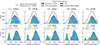 |
Fig. 3. Initial (top rows) and final (bottom rows) period distribution for the WD+MS binaries in models C1, C2, C3, C4 and C5 (α = 1.0 and fully conservative mass transfer, with different prescriptions for qcrit, following Table 2 – colored histograms). The colors indicate the type of interaction the system undergoes to end up as a WD+MS binary. The numbers in the bottom rows indicate the number of systems in the final distribution according to type of interaction. The dark gray line in the top plots shows the normalized period distribution for the entire simulated population (following Raghavan et al. 2010), including systems that do not end up as WD+MS binaries, but as double WDs, MS+MS binaries, mergers, and WD binaries with post-MS stars. All models are initialized with the same period distribution. The final period distribution of the WD+MS binaries are quite different between the models, indicating a strong dependence on mass transfer stability assumptions. |
Figure 3 also shows the relative number of systems in each COSMIC model broken down by evolutionary channel: no mass transfer, stable RLOF mass transfer, and CEE, with each channel colored by the type of interaction the system went through during its evolution. The majority of systems, for all models, become a WD+MS system without ever interacting (blue histogram); these systems have the longest orbital periods, as it is necessary that they be in wide orbits to avoid interaction in the first place. In all models, the systems that end up with the shortest periods are those that undergo CEE. Our choice of qset affects both the number of WD+MS binaries that undergo stable RLOF or CEE as well as their period distributions. Generally, stable mass transfer leads to longer periods. However, binaries that undergo CEE but have longer initial periods can have present day periods that are similar to binaries that go through stable mass transfer but originate with shorter periods.
Our models with qset = 1 follow the widely used prescription of critical mass ratio for unstable mass transfer (qcrit) from Claeys et al. (2014). In models with qset = 2, we explore a prescription where mass transfer occurring while the donor is in the AGB phase is more prone to stability, as the qcrit value for this evolutionary stage is higher. For models with qset = 3, mass transfer is more stable during the FGB phase, for models with qset = 4, during the TAGB phase, and finally for the entire GB in qset = 5 (see Table 2). As Figure 3 indicates, there is little variation in the WD+MS binary period distribution between models with qset = 1 and 2 within a given model family. This result is expected: low-mass stars (≤2 M⊙) are not expected to fill their RLs in the AGB phase, but in the FGB phase, where their cores become degenerate and their envelopes swell to much larger radii. Given the prevalence of low-mass stars in the initial mass function, systems undergoing mass transfer in the early AGB are expected to be less common, which likely explains the limited impact of increasing qcrit in this phase. Discrepancies between the models are more significant for qset = 3, 4 and 5. In particular, qset = 3 produces a much higher fraction of stable systems than the other prescriptions, and a lower mean orbital period. A value of qset = 4 also yields a larger number of stable systems in all model families, but the period distribution is wider, with a high density of systems around 1000 days, and some outliers with shorter periods, of the order of tens of days. This is because the WD+MS binary progenitors for qset = 3 that undergo stable mass transfer originate in shorter orbital periods compared to the stable mass transfer WD+MS binary progenitors in qset = 4. As expected, qset = 5 yields a larger number of stable systems, with a clear separation between the period regimes of stable RLOF and CEE products. The increased mass transfer stability in these models leads to a higher fraction of the population experiencing mass ratio reversal, particularly in models with fully conservative accretion (B, C and E). This reversal produces a gap in the ΔRVmax distribution in models B and C where there is no overlap between stable and unstable mass transfer products.
The accretion limit, β, has a limited impact on the final period distributions. There is a slight decrease in the number of systems that remain stable between the A and D models (β = 0.0 – i.e., nonconservative accretion) and the B, C and E models (β = 1.0 – i.e., fully conservative). The final period distribution of the interacting systems becomes less extended in all models with β = 1.0 compared to models with β = 0.0. Models C have a larger value for the common envelope ejection parameter (α = 1.0) than models A and B, meaning that all the change in orbital energy of the system is used to expel the envelope of the donor. Models D and E have α = 5.0, where an additional source of energy is used to remove the envelope. Because ejection is more easily achieved, more systems manage to avoid merging, increasing the overall size of the population of WD+MS binaries formed via CEE. The number of systems that merge in our COSMIC simulations increases the more conservative the mass transfer is, as the orbits shrink more effectively due to the conservation of angular momentum.
Figure 4 shows histograms of the period distribution for only the systems that undergo mass transfer (whether stable or unstable) in each model where the color indicates different model choices. The top panel shows the dependence of the period distribution on qset, keeping α and β fixed. There is a noticeable region with a low density of systems in the period distribution between ∼200 and ∼1000 days in all model families, with the clear exception of models A3 and A5. This absence of a gap is true for all models in families 3 and 5 and for models with high α (families D and E – see middle and bottom panels of Figure 3). The period gap is produced by the boundary between stable and unstable mass transfer. The systems that fall bellow this boundary have the necessary conditions (mass, radius and separation) to experience CEE, where mass and angular momentum transfer tighten the orbit of the system on a dynamical timescale. The differences in the size and exact position of the gap in period space depend, therefore, on the mass ratio threshold for unstable mass transfer, qcrit. In models with qset = 1, 2 and 4, FGB stars have a qcrit set by Eq. (1), which gives values in the range of 0.7–1.5. In contrast, models with qset = 3 and 5 have this value set to 2.0, allowing more systems to end mass transfer without going into CEE, pushing the mean period of these systems to lower values, and closing the gap in orbital period.
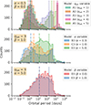 |
Fig. 4. Orbital period distribution of the WD+MS binaries that went through mass transfer, either stable or unstable, in our COSMIC models. The top panel shows the variation in the period distribution due to qcrit; middle panel shows the same, but due to α, and the bottom panel, due to β. The dashed lines show the median value of the period distribution considering only the stable mass transfer systems. The dash-dotted lines show the median period for the CEE systems. Values for the medians are shown in Table A.1. The largest changes in the period distribution occur when qset = 3, where the first ascension giant branch stars tend to have stable mass transfer, and qset = 5, where all giants are more stable. The main effect of increasing α is creating a post-CEE systems with larger periods, while the effect of β is nearly negligible. |
The vertical lines in Figure 4 represent the median of the period distributions for the products of stable mass transfer (dashed lines) and CEE (dash-dotted lines), with values shown in Table A.1. The median period does not change significantly for the products of CEE between models A and B. In model family C, the median of the final periods of systems that undergo CEE increases when compared to low-α models, with systems moving to wider periods in the 2–3 day range and populating the period gap, with the exception of model C2. This shows that the increased stability in the mass transfer during AGB phase (qset = 2) does not significantly impact the evolution of WD+MS binaries that form via CEE. High-α models D and E show an even clearer trend of CEE products with larger periods, with the mean for all qset jumping to tens of days, varying little among themselves, and closing the period gap present in lower α models. The middle panel of Figure 4 shows the dependence on α and clearly depicts this trend of increasing mean period of post-CEE systems. In the bottom panel of Figure 4 only β varies. Its effect is very limited, and the changes in the median of the period distributions are small.
For stable RLOF products, the effect of both α and β is not nearly as relevant as the effect of qset, with only slight variations in the median of the period distribution. Models A[1,2] and B[1,2] and models D[1,2] and E[1,2] show a trend of increasing median values indicating that their periods increase with β. Models [A,B]4 do not show the same behavior, with the median period instead decreasing slightly with β. The increase in period median is particularly noticeable between models D1 and E1, going from 92 to 1754 days. D1 has stable mass transfer binaries with short periods that are hidden in Figure 4, which skews the median to lower values. These systems originate from Hertzprung Gap donors that initiate mass transfer at short periods. Since β = 0.0 the final period is also short. E1 has β = 1.0, where during mass transfer, mass ratio reversal widens the binaries past 10 days.
The overall number of RLOF products increases greatly in model family 3. The period gap is filled up by the WD+MS binaries as stable mass transfer products for these models, which show only slight variations between each other, and thus do not seem to depend strongly on the value of either α or β. In models with qset = 5, the number of stable RLOF systems is the largest of all the models, and the median period of RLOF products is only higher than the median for qset = 3. For CEE products, the median period is larger than for other models when α = 0.3 (A and B), but decreases greatly for models with higher α (C, D, and E). This behavior of decreasing median period with α is the opposite of what we find for models with qset = 1, 2, 3, and 4 (see the values in Table 3). As the mass ratio threshold for CEE is higher in model family 5, there are fewer systems with lower-mass donors that initiate CEE. These lower-mass donors require smaller orbital energy changes, or alternatively lower envelope ejection efficiency, to survive CEE and retain larger orbits, as their envelopes are less massive. Thus, in model 5 there is a dearth of such CEE products. Instead, the higher-mass donors in model family 5 are more sensitive to changes in envelope ejection efficiency since there are more short-period post-CEE binaries that survive CEE without merging in the case of higher ejection efficiency. The combination of these effects pushes their median period to lower values as α increases for these models with higher stability.
4.2. Models versus observations: ΔRVmax distribution, periods, and WD masses
Our COSMIC models yield the final distributions of periods, eccentricities, and masses of the simulated systems. As is described in Section 3, we estimated the ΔRVmax distribution for each COSMIC model by supplying this information, plus a series of time lags, to an MC code. Figure 5 shows how the period distribution generated by a COSMIC model (in this case, model A3) translates into a ΔRVmax distribution using this method. The left panel shows the period distribution of model A3, colored by logarithmic period ranges. The stacked histogram on the right plot shows the ΔRVmax distribution resulting from 100 realizations of the MC code. The largest values of ΔRVmax correspond to the shortest period binaries, but the correlation between orbital period and ΔRVmax becomes less straightforward for lower ΔRVmax values, as ΔRVmax depends not only on period, but on the inclination of the system and on the timing of the observations: a system seen face-on will show no RV variation, and a system with a 50 day period will have a small ΔRVmax if its RV measurements are all taken within a span of only a couple of days.
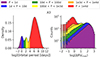 |
Fig. 5. Distribution of orbital periods (left panel) and ΔRVmax (right panel) for model A3, including systems that did not interact. There is an anti-correlation between period and ΔRVmax, but it is possible for short period systems to have small ΔRVmax, as ΔRVmax has a strong dependence on the inclination, eccentricity, and the time lag between radial velocity observations. Larger ΔRVmax are more unambiguously correlated with short period systems. |
4.2.1. Systems with orbital solutions from Gaia
Figure 6 shows the correspondence between orbital period and ΔRVmax for all models, overlaid with the values for the AGGC systems that have orbital solutions (large blue triangles for astrometric Gaia orbits, and large white inverted triangles for single line spectroscopic binaries, and large pink tilted triangles for systems with orbits derived from RV curves – see Table 1). The underlying 2D histograms show the log10-scaled spread of the ΔRVmax sampling over 100 MC realizations. The small symbols represent the mean ΔRVmax values for each of the binary systems, with the shape of the symbol indicating the type of mass transfer interaction (circles for RLOF, crosses for CEE, and squares for multiple RLOF phases). The region where ΔRVmax < 2 km/s is shaded gray in the plot. In this regime, individual ΔRVmax measurements can be affected by RV uncertainties (Badenes et al. 2018) that are not considered in our modeling (see Mazzola et al. 2020, Figure 3, Table 1 for a discussion). A version of this plot with all models is shown in Fig 6 in Appendix A.
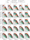 |
Fig. 6. Orbital periods and ΔRVmax for all models and observational data (triangles). Colors indicate the type of WD formed after mass transfer, and the markers indicate the type of mass transfer the system went through. Noninteracting systems are not shown. The shaded gray region indicates the region below ΔRVmax = 2km/s, where RV uncertainties dominate. The background squares show 2D log10-scaled histograms of all 100 MC realizations of the ΔRVmax distribution for each binary system in the model; the markers are the mean of the distribution for each binary. Models with qset = 3, models D and E and model A5 are the best matches to the data, showing more continuous period/ΔRVmax distributions. |
For values of ΔRVmax above a few kilometers per second the AGGC systems with Gaia orbital solutions show a continuous relation of periods and ΔRVmax. In contrast, as is discussed in Section 3 above, several COSMIC models show a gap (a region where no or only relatively few WD+MS systems are formed) in the orbital period distribution. As is seen in Figure 6, models [A,B,C]1 have a small gap around 1000 days, models [A,B,C] have a decrease around 300 days, and models [A,B,C]4 have a large gap between 100 and 1000 days. As already evidenced by the period distributions in Figure 4, the effect of qset is extremely relevant in determining the size, position, and intensity of this gap. In models with high α (D and E), only model D4 shows a gap, which is smaller than the one in models [A,B,C]4.
It is clear that models with qset = 3 and 5, and models in families D and E cover the same parameter space as the systems with Gaia orbits, while models [A,B,C][1,2,4] struggle to reproduce the data. We note that we have few systems with Gaia orbits, and that the 5 systems with ΔRVmax < 2 km/s had their ΔRVmax obtained from APOGEE observations taken within a few-day window, leading to a lower estimated ΔRVmax than expected from their periods.
Figure 6 also indicates the composition of the WD in our models. In COSMIC, whether the final WD is a helium (He), carbon/oxygen (CO), or oxygen/neon (ONe) WD is determined by its final mass as enforced by the amount of nuclear burning allowed in the stellar core, taking into account any mass transfer episodes. He WDs have masses lower than 0.45 M⊙, CO WDs between 0.45 and 1.05 M⊙, and ONe above 1.05 M⊙. A noted difference between models with qset = 3 and the rest is that in these models, the gap is filled with WDs of different origin and composition. For instance, in model C1 the only way the COSMIC simulations create systems with orbits of 100 to 1000 days is via CEE, and the resulting WD is always a CO WD; on the other hand, systems can form in that period space in models with qset = 3 via either RLOF or CEE, showing a mix of He and CO WDs. Thus, establishing the mass and composition of the WD in the observed systems in this region of the period/ΔRVmax plot could help determine which model provides the best description of the true WD+MS population.
The AGGC systems with orbital solutions from Gaia have estimates for the mass of MS star. Using these estimates and the RV semi-amplitude of the primary (K) measured by Gaia, we can infer the minimum mass of the WD companion. With this value, the composition of the WD can be estimated. While the correlation between WD mass and composition is not straightforward for products of binary interaction, we tentatively confront this estimated WD composition of the observed sample to the models.
Figure 7 compares the estimated mass of the MS star and period for the systems shown in Table 1 to models [A,B,C,D,E]3, favored by the ΔRVmax comparison (see Sect. 4.2). The colors represent the WD type (He, CO and ONe). As shown in Table 1, the estimate of the mass (and thus type) of the WD depends on the inclination of the orbit. As such, the WD types shown by the colors in Figure 7 relate to the minimum WD mass. Thus, systems that have a minimum WD mass corresponding to a He WD might not in fact have a He WD when the inclination is accounted for; these data are colored yellow in the Figure. Considering these effects, models A3 and D3 provide the best qualitative agreement with the data.
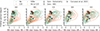 |
Fig. 7. Orbital period versus mass of the MS component of the WD+MS binary systems. The background KDE contours represent the model (from left to right, A3, B3, C3, D3, and E3). The triangles represent observational data from Table 1. The colors indicate the type of WD companion: teal for He, orange for CO, purple to ONe, and yellow for WDs that can be either He or CO depending on the inclination of the system. Models A3 and D3, both with β = 0.0, are the only models that can reproduce the large-period (P > 100 days), low-mass MS+He WD systems. |
There is a clear trend in the location of the He WD companions in the period range of 10-1000 days to shift to higher MS companion masses for increased β (A3 to B3, D3 to E3). The He WDs in this period range are all stable mass transfer products (see Figure 6). As the mass accretion becomes more efficient, less massive (He) WDs can only be formed if the MS donor does not lose too much of its mass in the mass transfer. Only models A3 and D3 (both with nonconservative mass accretion) can reproduce the He WDs in that period region found in the data. We note that the nature of these WDs as He WDs is an estimate based on the available data. Confirming the mass of these WDs will provide constraints to the mass transfer efficiency for these models.
Increasing the number of WD+MS systems with well-measured masses, orbital periods, and temperatures will facilitate a more robust statistical comparison between models and data in the future. For example, the WD binaries pathway survey, beginning in 2016 (Parsons et al. 2016), has confirmed both individual WD+MS binaries and populations obtained through both spectroscopic and astrometric survey data with spectroscopic follow-up studies.
4.2.2. Systems with only ΔRVmax from APOGEE
We also compared the ΔRVmax distributions predicted by our COSMIC models with the entire AGGC sample of WD+MS systems using histograms and cumulative distribution functions (CDF). Histograms can be complicated to interpret due to binning and cutoff effects (see Appendix B), but all models in families 1, 2, and 4 peak around 1.5 < log(ΔRVmax/(km/s)) < 1.8 and decrease as ΔRVmax increases, while models in family 3 have a flatter distribution after the peak. Figure A.1 shows the ΔRVmax histograms for the 100 MC realizations for all models (light green blocks) and the AGGC ΔRVmax data (dots) where the width of the blocks represents the 90% confidence region for each bin. The ΔRVmax distribution histograms cover the range from 5 to 1000 km/s. The low end cut on 5 km/s is motivated by uncertainties in the ΔRVmax measurements from APOGEE, and the fact that the large period systems present in our models that dominate in low ΔRVmax are likely not present in the AGGC data, as wider binaries are more difficult to detect. With this cut, the number of AGGC data points is 98. Thus, we divided the distribution in  log-spaced bins for our analysis. The data peaks close to log(ΔRVmax) = 2.0, suffers a decrease, and plateaus for log(ΔRVmax) < 1.5.
We used the Anderson-Darling (AD) statistical test on the ΔRVmax cumulative distributions of the models and data, comparing the data with the mean CDF of all MC realizations for each model. Figure 8 shows the results of the AD test for all COSMIC models. The null hypothesis that the data and models were sampled from the same underlying distribution is rejected by the AD test at the a certain significance level when the AD statistic is larger than a given critical value. If the AD statistic exceeds 0.325, the null hypothesis can be rejected at the 25% level; if it exceeds 1.226, at the 10% level; 1.961 at the 5% level, 2.718 at the 2.5% level, 3.752 at the 1% level, 4.592 at the 0.5% level, and finally 6.546 at the 0.1% level. Therefore, models with an AD statistic larger than 6.546 strongly reject the hypothesis that the two samples come from the same underlying distribution, while models with a statistic lower than 0.325 cannot reject the null-hypothesis. For models A[1,2,4], B[1,2,3,4,5] and C[2,4,5], the hypothesis can be rejected at the 0.1% level. Models C1 and A3 are rejected at the 0.5% level, and models C3 and A5 at the 2.5% level. Models [D,E][1,2,4] can be rejected only at the 10% level. Finally, models [D,E][3,5] cannot be rejected.
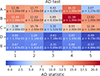 |
Fig. 8. AD statistics for the comparison of the ΔRVmax distribution of COSMIC models to data. Histograms are shown in Figure A.1. AD statistic lower than 6.546 cannot be discarded as being sampled from the same underlying distribution. Models with α = 5.0 (families D and E) and models [A,C]3 and A5 are the best matches to the data. |
In addition to the AD test, we also considered different measurements of statistical distance between the data and the models. We varied the number of bins and the lower end cutoff of the ΔRVmax distribution to guarantee that our results are independent of these factors. The results of these tests are shown in Appendix B, Figure B.1.
As the results of all statistical tests performed indicate, we conclude that the only models that cannot be outright rejected statistically are models with high α (families D and E), and models A[3,5] and C3, where the critical mass ratio for the onset of unstable mass transfer, qcrit, for FGB stars (in A3 and C3) or for the entire GB (A5) is fixed at 2.0. This value is higher than the one assumed in the widely used qcrit prescriptions of Hurley et al. (2002) and Claeys et al. (2014). Our higher value indicates that stars that fill the Roche-lobe in the FGB in particular are more prone to undergo stable mass transfer. We note, however, that a larger sample would be required to draw more robust statistical comparison to our BPS models.
5. Discussion
Determining the stability of mass transfer in binaries is crucial to understand the formation channels and subsequent evolution of post-RLOF systems. Given the complexity of this problem, the classical approach has been to estimate the response of mass transfer based on simplifications to the structure of the donor star and the assumption that its response to mass transfer is adiabatic. Thus, donors with radiative envelopes would tend toward stability, while giants with convective envelopes would quickly turn unstable (Hjellming & Webbink 1987). Many works in the past couple of decades have demonstrated that these simplifications underestimate the stability of mass transfer for many mass ranges. From the observational side, Leiner & Geller (2021), for instance, finds that the number of blue stragglers found in clusters on Gaia DR2 cannot be reproduced by COSMIC using the qcrit prescriptions of Hurley et al. (2002) or Hjellming & Webbink (1987).
Theoretical studies have also found indications that the instability criteria need to be reevaluated. Pavlovskii & Ivanova (2015)’s models of mass transfer find higher stability for giant donors when the response of the superadiabatic layers of the star to mass loss is considered in stellar evolution models. The mass loss sequences of Ge et al. (2010, 2020), based on more realistic models of stellar interiors, yield mass-radius relations that map the threshold of thermal to dynamical timescale mass loss for a wide range of mass ratios. Their results indicate that donors on the RGB and AGB tend to be more stable (i.e., harder to begin rapid mass transfer and go into CEE) than previous models indicated.
The work of Temmink et al. (2023) delves deep into the issue of mass transfer with post-MS donors. Using the stellar evolution code MESA (Paxton et al. 2011; Jermyn et al. 2023, and others), they follow the evolution of the donor until it fills its Roche lobe without imposing a fully adiabatic response on the star, which prevents a too-rapid expansion of the convective envelope. Their results indicate that giant donors undergo stable mass transfer for a wider range of mass ratios than the widely used prescription of Hurley et al. (2002). However, rapid BPS codes continue to use these prescriptions to determine the threshold of stability of their systems due to both software development lag times and lack of information on stellar interior structures due to the use of fitting formulae.
Comparing the ΔRVmax and period distributions of our COSMIC models with the AGGC data shows that several models are unable to reproduce the general trends seen in the data. In Figure 6, models [A,B,C][1,2,4] and [D,E]4 predict a gap in the period distribution that is not seen in the data. Models [B,C]5 show a less significant gap that only exists in ΔRVmax space; this is due to the larger mass ratios the stable RLOF products reach for β < 0.5 in contrast with CEE products with the same period. These models are disfavored as good representations of the population of WD+MS binaries of AGGC by the results of the ΔRVmax distribution (Figure A.1). On the other hand, models with qset = 3 and models with α = 5.0 appear to more accurately capture observed features in the data. While our findings rely on simple assumptions for the stability of mass transfer, our flexible approach arrives to the same conclusions found in detailed stellar evolution modeling. Similar tests applied to larger datasets in the future may be able to connect theoretical predictions to observations in order to apply constraints on mass transfer across a wide range of the binary population parameter space.
The distribution of WD and MS companion masses with period shown in Figure 7 offers even more insight, although the masses are more uncertain than the ΔRVmax and period estimates. Of the models favored by the ΔRVmax distribution, only A3 and D3 cover the same parameter space as the data in donor masses and period for He WDs with periods larger than 100 days. This result indicates a preference for low β, or less conservative mass transfer (Figure 7). By increasing α, binary systems with He WDs are formed in a wider range of periods, reaching as high 100 days, also creating an overall larger population of WD+MS binaries. Even so, the data show He WDs with periods on the order of several hundreds to nearly 1000 days, which can only be reproduced in our models by increasing qcrit for the onset of instability in first ascent giant stars (qset = 3).
High α, or extremely efficient envelope ejection in CEE, is preferred by our results, as it provides a ΔRVmax distribution that matches the high ΔRVmax end of the AGGC distribution (see Figure A.1). In practice, this means that the AGGC data require that a larger fraction of post-CEE systems (which dominate the high end of the ΔRVmax distribution – see Figure A.2) have larger periods. Since models with lower α over-predict the number of short periods, a large α is preferred. Still, α = 5.0 is significantly higher than the “standard” value of 0.3 (i.e., Zorotovic et al. 2010; Scherbak & Fuller 2023). An α > 1 requires that all of the change in orbital energy plus an additional source of energy be used to expel the envelope. This extra energy would likely come from thermal energy, recombination energy from the expansion of the envelope (Zorotovic et al. 2014; Nandez & Ivanova 2016; Ivanova 2018), and nuclear energy due to interaction between the two stars (Podsiadlowski et al. 2010).
Whether or not any additional energy is necessary to create post-CEE WD+MS binaries with periods on the order of tens of days is currently a matter of debate. The catalog of WD+MS candidate binaries compiled by Shahaf et al. (2023) from the third Gaia data release offers insight. Follow up work in Yamaguchi et al. (2024a) and Yamaguchi et al. (2024b) seek to validate the orbits of WD+MS binaries in these catalogs for massive ONe WDs (the former) and for more standard CO WDs (the latter). In both studies, the formation pathways for the observed systems are considered by simulating the evolution of single stars up to and through the thermal pulses on the AGB. Both papers find that the observed wide orbital periods, between 100 to 1000 days, can be produced by WD progenitors that initiate the CEE with low envelope binding energies due to the highly evolved donor star.
In the case of the ONe WD progenitors, the inclusion of recombination energy leads to the observed periods (Yamaguchi et al. 2024a). In the case of the CO WD progenitors, long period post-CEE WD+MS binaries can be formed without the need for the additional recombination energy, even for low values of α. However, while recombination energy is not strictly required to explain the long period post-CEE WD+MS binaries, their models show that it dominates the internal energy in the outer envelope of the donor during the TAGB phase, and therefore should play a significant role in the envelope ejection. Including recombination energy also produces long period binaries for a wider range of initial parameters.
Another important point is that the envelope-structure parameter, λ, changes significantly when recombination energy is included in the modeling. This is clearly illustrated by Figure 13e of Yamaguchi et al. (2024b), which shows the changes in λ during the TAGB phase for models with and without recombination energy. During the thermal pulses, λ oscillates around values near 0.5 for the model with no recombination, while the value goes from -1 (i.e., the envelope is unbound) up to 5 when recombination is considered.
In COSMIC, we used the αλ prescription for CEE. As in BSE, COSMIC sets λ based on the calculations of Claeys et al. (2014). While we only explored different values for α between our models, these two parameters are degenerate: the same effect could be achieved by modifying λ instead. Thus, it is more accurate to interpret our results for α as the combined effect of αλ as well as potential additional energy sources. Our results indicate that either CEE donors have much lower envelope binding energies or that recombination energy is necessary to explain the distribution of ΔRVmax. In particular the higher end, dominated by short period binaries, which are overpredicted by our low α models. This result is consistent with Yamaguchi et al. (2024b)’s interpretation that recombination energy does play a significant role in the TAGB phase, making them more efficient at forming WD+MS binaries with wider periods. The significant effect of the recombination energy on λ during the TAGB phase shown by Yamaguchi et al. (2024b)’s models indicates that its implementation in BPS codes are unlikely to capture the full range of λ values that occur during the late-stage evolution of WD progenitors. Given the degeneracy with α, it is possible that discrepancies between values of α found in different BPS studies are actually due to changes in λ between (and during) different evolutionary phases of the donor.
The recent work of Torres et al. (2025) uses inverse population synthesis techniques to reconstruct the evolution of WD+MS systems. Their modeling uses the αλ prescription, but they only use orbital energy to unbind the envelope, which implicitly enforces a null internal energy contribution. This means that α is limited to 1 in their results. Applying their algorithm to a sample of 30 eclipsing WD+MS binaries, they find a strong correlation between the mass of the WD progenitor and α, and that a single value of α cannot reconstruct all systems in their sample. We propose that this correlation in α is caused by the degeneracy between α, λ, and the mass of the WD progenitor, as these parameters are connected via the binding energy of the envelope and orbital separation at the onset of the first RLOF. The limitation of α ≤ 1 and assumed prescription for λ requires a change in the mass of the WD progenitor to account for the required changes in envelope binding energy. Our simulations choose the same prescription for λ, but do allow for α > 1 (and find a slight preference for α = 5). While we do not account for possible correlations between mass and α, the assumptions for λ do account changes in binding energy due to radial expansion of the WD progenitor. If, as suggested by Yamaguchi et al. (2024a,b), our applied assumptions for λ overpredict the envelope binding energy, the correlations found by Torres et al. (2025) may be accounted for naturally with upgraded assumptions to stellar physics.
In another study, Belloni et al. (2024) uses the population synthesis code BSE (Hurley et al. 2002) to simulate post-CEE binaries containing ONe WDs to compare with massive WD binaries reported in Yamaguchi et al. (2024a). Belloni et al. (2024) find that wide ONe WD binaries could be formed assuming only efficient envelope ejection, with no extra source of energy required. This is achieved by allowing the WD progenitors to enter CEE as a highly evolved TAGB star, where the donor star radius is larger and there has been significant mass loss due to winds than at the AGB phase. In this case, the amount of orbital energy required to eject the envelope is less due to lower binding energies. Future studies that consider larger simulations may be able to provide a more comprehensive comparison, but are currently outside the scope of this paper.
Finally, we consider two important caveats to this work. First, our results assume that AGGC contains a pure sample of WD+MS binaries. However, as was mentioned in Section 2, the catalog might be contaminated by single MS stars with high chromospheric activity, which are incorrectly assigned as WD+MS binaries by their excess in FUV. If indeed this is the case for a significant part of our dataset, it could significantly bias our results. Future studies using larger complementary datasets could either uncover this bias or help validate our findings.
We also note that we only considered one assumption for how mass that is not accreted in stable mass transfer is treated. Future studies could explore different angular momentum loss assumptions where higher rates of angular momentum loss would lead to shorter periods after RLOF, potentially increasing the effects of stable mass transfer in our model family 3. However, we expect this effect to be less dominant than our assumptions for the stability of mass transfer and CEE since the majority of the WD+MS population is formed through CEE.
6. Conclusion
In this work, we compare WD+MS binaries from the APOGEE-Galex-Gaia catalog with synthetic binary populations calculated with the BPS code COSMIC. Because the AGGC offers the distinct advantage of a large and homogeneous sample of WD+MS binaries with multiple high-quality RV measurements for each system, we used their ΔRVmax measurements (and the full orbital solutions for some systems) to calibrate the binary mass transfer parameters used in COSMIC. We explored a range of values for the common envelope ejection efficiency (α), the accretion limit (β), and the critical mass ratios that define the onset of unstable mass transfer (qcrit) used in COSMIC, which are also standard parameters in other BPS codes.
Overall, model D3 best describes both the ΔRVmax distribution (Figures 6 and A.1) and the measured WD masses in the AGGC data (Figure 7). This suggests a preference for qset = 3 (defined in Table 2) such that stable mass transfer during RLOF for FGB donor stars occurs for mass ratios up to qcrit = 2.0, α = 5.0, and β = 0.0. We summarize these preferences below.
-
More stable mass transfer on the FGB: We disfavor models in which FGB stars go into unstable mass transfer with qset other than 3 when α < 5. Such models either underestimate (see models [A,B,C][1,2,4]) or overestimate (models [A,B,C]5) the number of small ΔRVmax (long-period binaries –see histograms in Figure A.1). This result indicates that mass transfer from donor stars on the FGB is more stable than the widely used qcrit prescription of Claeys et al. (2014). It also corroborates recent studies that find increased mass transfer stability in giant stars in both data and models (i.e., Temmink et al. 2023).
-
High α: In the ΔRVmax comparison, there is a preference for models with a high common envelope ejection efficiency (α), but the statistical significance is low, and models with qset = 3 and lower α should not be completely excluded. The preference for high-α models indicates that the inclusion of some other energetic source during envelope ejection is necessary. However, the α parameter is degenerate with the envelope structure parameter, λ. It might be the case that our results suggest that donor envelopes are less bound than the assumptions in COSMIC. Following Yamaguchi et al. (2024b), this may be the case during the thermally pulsing AGB phase, where λ varies widely, and in a manner not accounted for in BPS codes.
-
Low mass transfer efficiency: When information on the minimum WD mass drawn from full orbital solutions is considered, models with a low mass transfer efficiency (β) are preferred, as they are the only models that produce He WDs in the same parameter region as the data.
We require more precise orbital solution and mass estimates to draw more robust conclusions on the mass transfer parameters of the population of WD+MS binaries. Comparing ΔRVmax distributions provides a general idea of the trends of the distribution in period space, but the addition of precisely measured orbital periods of these observed systems to compare with the COSMIC models will allow direct constraints to be imposed on mass transfer assumptions. More accurate WD mass estimates will also further constrain these assumptions. At present, the ΔRVmax distribution is the most effective indicator of the effect of CEE assumptions for our sample, but it is dominated by changes to our assumptions for mass transfer stability. Additional precise measurements for the periods and masses of WD binaries will allow for more precise constraints that can help discriminate between values of β (Figure 7).
Our results showcase that large, homogeneous datasets can be used to constrain parameters in rapid BPS codes that can be directly connected theoretical models for binary evolution. They also show that certain commonly used prescriptions, such as the αλ for CEE and the qcrit of Hurley et al. (2002), should be revised to take into account the most recent results of stellar evolution modeling. In particular, careful treatment of envelope binding energies rather than variable envelope ejection efficiencies may be a direct route to understanding post-CEE WD binaries.
The release of Gaia DR4 will provide orbital solutions for many more WD+MS binaries, and for other post-mass transfer systems as well. When these data are available, our comparison to BPS models can be reassessed for more accurate limits on the mass transfer parameters. In the longer term, the Laser Interferometer Space Antenna (LISA) mission will lead to the detection and characterization of thousands of Galactic gravitational wave sources including close double WD binaries and other post-interaction compact binaries. Comparing these data with BPS models will produce constraints on the mass transfer parameters for a wider range of initial conditions (e.g., Thiele et al. 2023; Delfavero et al. 2025).
Acknowledgments
This work was initiated at the Kavli Summer Program in Astrophysics 2023, hosted at the Max Planck Institute for Astrophysics. We thank the Kavli Foundation and the MPA for their support. ACR acknowledges support from ESO and its studentship program. ACR is grateful to Selma de Mink and Stephen Justham for helpful comments and discussion during the development of this project, and Alex Carciofi for continued support. ACR, KB and CB are also grateful to the AGGC collaboration for useful discussions on the manuscript. CB, BA, and SM acknowledge support from NSF-AST grant 2307865. KE acknowledges support from NSF grant AST-2307232.
References
- Abdurro’uf, Accetta, K., Aerts, C., et al. 2022, ApJS, 259, 35 [NASA ADS] [CrossRef] [Google Scholar]
- Althaus, L. G., Córsico, A. H., Isern, J., & García-Berro, E. 2010, A&ARv, 18, 471 [NASA ADS] [CrossRef] [Google Scholar]
- Anguiano, B., Majewski, S. R., Stassun, K. G., et al. 2022, AJ, 164, 126 [CrossRef] [Google Scholar]
- Badenes, C., Mazzola, C., Thompson, T. A., et al. 2018, ApJ, 854, 147 [NASA ADS] [CrossRef] [Google Scholar]
- Belczynski, K., Kalogera, V., Rasio, F. A., et al. 2008, ApJS, 174, 223 [Google Scholar]
- Belloni, D., Zorotovic, M., Schreiber, M. R., et al. 2024, A&A, 686, A61 [NASA ADS] [CrossRef] [EDP Sciences] [Google Scholar]
- Bianchi, L., Shiao, B., & Thilker, D. 2017, ApJ, 230, 24 [NASA ADS] [Google Scholar]
- Breivik, K., Coughlin, S., Zevin, M., et al. 2020, ApJ, 898, 71 [Google Scholar]
- Claeys, J. S. W., Pols, O. R., Izzard, R. G., Vink, J., & Verbunt, F. W. M. 2014, A&A, 563, A83 [NASA ADS] [CrossRef] [EDP Sciences] [Google Scholar]
- Corcoran, K. A., Lewis, H. M., Anguiano, B., et al. 2021, AJ, 161, 143 [Google Scholar]
- De Marco, O., Passy, J.-C., Moe, M., et al. 2011, MNRAS, 411, 2277 [CrossRef] [Google Scholar]
- Delfavero, V., Breivik, K., Thiele, S., O’Shaughnessy, R., & Baker, J. G. 2025, ApJ, 981, 66 [Google Scholar]
- Ge, H., Hjellming, M. S., Webbink, R. F., Chen, X., & Han, Z. 2010, ApJ, 717, 724 [NASA ADS] [CrossRef] [Google Scholar]
- Ge, H., Webbink, R. F., Chen, X., & Han, Z. 2020, ApJ, 899, 132 [NASA ADS] [CrossRef] [Google Scholar]
- Halbwachs, J.-L., Pourbaix, D., Arenou, F., et al. 2023, A&A, 674, A9 [NASA ADS] [CrossRef] [EDP Sciences] [Google Scholar]
- Hjellming, M. S., & Webbink, R. F. 1987, ApJ, 318, 794 [Google Scholar]
- Hurley, J. R., Pols, O. R., & Tout, C. A. 2000, MNRAS, 315, 543 [Google Scholar]
- Hurley, J. R., Tout, C. A., & Pols, O. R. 2002, MNRAS, 329, 897 [Google Scholar]
- Ivanova, N. 2018, ApJ, 858, L24 [NASA ADS] [CrossRef] [Google Scholar]
- Ivanova, N., Justham, S., Chen, X., et al. 2013, A&ARv, 21, 59 [Google Scholar]
- Jermyn, A. S., Bauer, E. B., Schwab, J., et al. 2023, ApJS, 265, 15 [NASA ADS] [CrossRef] [Google Scholar]
- Koester, D. 2010, Mem. Soc. Astron. It., 81, 921 [NASA ADS] [Google Scholar]
- Kroupa, P. 2001, MNRAS, 322, 231 [NASA ADS] [CrossRef] [Google Scholar]
- Kurucz, R. L. 1979, ApJS, 40, 1 [NASA ADS] [CrossRef] [Google Scholar]
- Leiner, E. M., & Geller, A. 2021, ApJ, 908, 229 [Google Scholar]
- Lindegren, L., Klioner, S. A., Hernández, J., et al. 2021, A&A, 649, A2 [EDP Sciences] [Google Scholar]
- Majewski, S. R., Schiavon, R. P., Frinchaboy, P. M., et al. 2017, AJ, 154, 94 [NASA ADS] [CrossRef] [Google Scholar]
- Mazzola, C. N., Badenes, C., Moe, M., et al. 2020, MNRAS, 499, 1607 [CrossRef] [Google Scholar]
- Nandez, J. L. A., & Ivanova, N. 2016, MNRAS, 460, 3992 [Google Scholar]
- Parsons, S. G., Rebassa-Mansergas, A., Schreiber, M. R., et al. 2016, MNRAS, 463, 2125 [Google Scholar]
- Pavlovskii, K., & Ivanova, N. 2015, MNRAS, 449, 4415 [Google Scholar]
- Paxton, B., Bildsten, L., Dotter, A., et al. 2011, ApJS, 192, 3 [Google Scholar]
- Podsiadlowski, P., Ivanova, N., Justham, S., & Rappaport, S. 2010, MNRAS, 406, 840 [NASA ADS] [Google Scholar]
- Pols, O. R., Schröder, K.-P., Hurley, J. R., Tout, C. A., & Eggleton, P. P. 1998, MNRAS, 298, 525 [Google Scholar]
- Postnov, K. A., & Yungelson, L. R. 2014, Liv. Rev. Relativity, 17, 3 [NASA ADS] [CrossRef] [Google Scholar]
- Queiroz, A. B. A., Anders, F., Chiappini, C., et al. 2023, A&A, 673, A155 [NASA ADS] [CrossRef] [EDP Sciences] [Google Scholar]
- Raghavan, D., McAlister, H. A., Henry, T. J., et al. 2010, ApJS, 190, 1 [Google Scholar]
- Scherbak, P., & Fuller, J. 2023, MNRAS, 518, 3966 [Google Scholar]
- Shahaf, S., Bashi, D., Mazeh, T., et al. 2023, MNRAS, 518, 2991 [Google Scholar]
- Temmink, K. D., Pols, O. R., Justham, S., Istrate, A. G., & Toonen, S. 2023, A&A, 669, A45 [NASA ADS] [CrossRef] [EDP Sciences] [Google Scholar]
- Thiele, S., Breivik, K., Sanderson, R. E., & Luger, R. 2023, ApJ, 945, 162 [NASA ADS] [CrossRef] [Google Scholar]
- Toonen, S., Hollands, M., Gänsicke, B. T., & Boekholt, T. 2017, A&A, 602, A16 [NASA ADS] [CrossRef] [EDP Sciences] [Google Scholar]
- Torres, S., Gili, M., Rebassa-Mansergas, A., et al. 2025, A&A, 698, A173 [NASA ADS] [CrossRef] [EDP Sciences] [Google Scholar]
- Wright, E. L., Eisenhardt, P. R. M., Mainzer, A. K., et al. 2010, AJ, 140, 1868 [Google Scholar]
- Yamaguchi, N., El-Badry, K., Fuller, J., et al. 2024a, MNRAS, 527, 11719 [Google Scholar]
- Yamaguchi, N., El-Badry, K., Rees, N. R., et al. 2024b, PASP, 136, 084202 [Google Scholar]
- Zorotovic, M., Schreiber, M. R., Gänsicke, B. T., & Nebot Gómez-Morán, A. 2010, A&A, 520, A86 [NASA ADS] [CrossRef] [EDP Sciences] [Google Scholar]
- Zorotovic, M., Schreiber, M. R., & Gänsicke, B. T. 2011, A&A, 536, A42 [NASA ADS] [CrossRef] [EDP Sciences] [Google Scholar]
- Zorotovic, M., Schreiber, M. R., García-Berro, E., et al. 2014, A&A, 568, A68 [NASA ADS] [CrossRef] [EDP Sciences] [Google Scholar]
Appendix A: Summary table and figures of full model set of COSMIC simulations
Figure A.1 shows the histograms for all COSMIC models compared to the ΔRVmax measurements from the AGGC. Models in families 1, 2, and 4 cannot reproduce the low ΔRVmax plateau. The low and middle α models, [A,B,C][1,2], are able to reproduce the rapid rise in the in log(ΔRVmax) between 2 and 3 km/s, which high-α models [D,E][1,2] underestimate. Models with qset = 4 behave similarly, but only model C4 captures the behavior of the high ΔRVmax peak; models [A,B]4 overestimate the number of systems, while models [D,E]4 underestimate them. Models [A,B,C]5, on the other hand, overestimate the number of low ΔRVmax systems, and predict a drop in the number of intermediate ΔRVmax that is not seen in the data. Undoubtedly, models with qset = 3 are the ones that best describe the data, corroborating the results shown in Section 4.2.1, where these models are shown to reproduce the periods, ΔRVmax, and WD masses of the sample of WD+MS with Gaia orbital solutions.
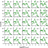 |
Fig. A.1. ΔRVmax histograms for 100 MC realizations for all 25 COSMIC models (light green blocks) and the AGGC ΔRVmax data (dots); the width of the blocks represents the 90% confidence region for each bin. The ΔRVmax distribution histograms cover the range from 5 to 1000 km/s, with 10 bins. Models with low α and qset ≠ [3,5] ([A,B,C][1,2,4]) tend to underestimate the number os systems with lower ΔRVmax, and overestimate the systems with high ΔRVmax; models with low α and qset = 5 greatly overestimate the number of systems with low ΔRVmax. |
Figure A.2 shows the mean ΔRVmax distribution of all models (same as the full line in the histograms of Figure 6), colored by the type of interaction. The shaded gray region is our chosen ΔRVmax cutoff of 5km/s. The post-CEE systems dominate the distribution, as expected. This explains the strong dependence of our results on CEE parameters α and qset, and the much weaker effect exerted by β. The larger RV errors in the low ΔRVmax regime make the region dominated by stable mass transfer WD+MS binaries difficult to probe with only ΔRVmax.
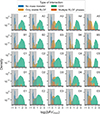 |
Fig. A.2. ΔRVmax distribution for all 25 COSMIC models, colored by the type of interaction the system suffered. The shaded gray region is the 5km/s cut. The ΔRVmax > 5km/s region is dominated by post-CEE WD+MS binaries. |
Table A.1 offers more detailed information on the outcomes of the binaries in each of our COSMIC models. The table shows the number of systems that end up as WD+MS binaries, WD+non-MS star, double WD (DWD), mergers, and other configurations (such as MS+MS binaries). We also show the number of WD+MS binaries that form our sample once the cuts in UV magnitude are applied. The last two columns show the values of the median of the period distribution of the final sample, separated by the time of mass transfer the system undergoes. These values are shown as the dotted and dashed lines in Figure 4. The table is discussed in Sect. 4.
Additional information on COSMIC models.
Appendix B: Statistical tests, cutoff and binning effects
We performed several statistical tests to quantitatively compare the ΔRVmax distributions of the AGGC data and our COSMIC populations. When comparing the histograms, we calculated a Poisson likelihood (as the sum of the log of the Poisson probability mass function in each bin); the total variation distance, defined as
 (B.1)
(B.1)
where D and M are the counts of systems in each bin, i; and the Hellinger distance,
 (B.2)
(B.2)
We further consider the Manhattan, or city block distance,
 (B.3)
(B.3)
and the Euclidean distance
 (B.4)
(B.4)
We also explore different cutoff choices for low ΔRVmax and binning for the histograms. A summary of these choices for all metrics is shown in Figure B.1. All metrics, regardless of cutoff and binning choice, appear to slightly prefer models with qset = 3 as the most similar to the AGGC ΔRVmax distribution.
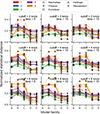 |
Fig. B.1. Normalized statistical distances between our COSMIC models and the AGGC ΔRVmax distribution, with varying cutoff values for the minimum ΔRVmax and number of bins in the compared histograms (histograms shown in Figure 6). The colors indicate the qset value, while the markers indicate different statistical measures. Models with qset = 3 and models with α = 5.0 (D and E) consistently show lower distances to the observational data, which corroborates our finding that these models are better matched to the available data. |
All Tables
All Figures
|
Fig. 1. Overview of the WD binaries in the APOGEE-Gaia-Galex catalog (AGGC). The left panel shows the full APOGEE dataset in blue and the companions of WDs in orange. The right panel shows the ΔRVmax distribution for different cuts in the data: MS+MS binaries from the full APOGEE dataset in blue, all WD binaries in the AGGC in green, and WD+MS binaries in black. The full APOGEE dataset contains 455796 targets; the MS binaries in that sample number 151266. The full AGGC has 1157 candidate WD binaries, while the WD+MS systems number 588. |
| In the text | |
|
Fig. 2. Schematic of the possible evolutionary paths through which a binary system can go to become a WD+MS binary. The system can either not interact, or go through RLOF mass transfer, which can in turn be stable or unstable, leading to a common envelope phase. The imprints of their evolution can be seen in the final masses and orbital period of the systems. |
| In the text | |
|
Fig. 3. Initial (top rows) and final (bottom rows) period distribution for the WD+MS binaries in models C1, C2, C3, C4 and C5 (α = 1.0 and fully conservative mass transfer, with different prescriptions for qcrit, following Table 2 – colored histograms). The colors indicate the type of interaction the system undergoes to end up as a WD+MS binary. The numbers in the bottom rows indicate the number of systems in the final distribution according to type of interaction. The dark gray line in the top plots shows the normalized period distribution for the entire simulated population (following Raghavan et al. 2010), including systems that do not end up as WD+MS binaries, but as double WDs, MS+MS binaries, mergers, and WD binaries with post-MS stars. All models are initialized with the same period distribution. The final period distribution of the WD+MS binaries are quite different between the models, indicating a strong dependence on mass transfer stability assumptions. |
| In the text | |
|
Fig. 4. Orbital period distribution of the WD+MS binaries that went through mass transfer, either stable or unstable, in our COSMIC models. The top panel shows the variation in the period distribution due to qcrit; middle panel shows the same, but due to α, and the bottom panel, due to β. The dashed lines show the median value of the period distribution considering only the stable mass transfer systems. The dash-dotted lines show the median period for the CEE systems. Values for the medians are shown in Table A.1. The largest changes in the period distribution occur when qset = 3, where the first ascension giant branch stars tend to have stable mass transfer, and qset = 5, where all giants are more stable. The main effect of increasing α is creating a post-CEE systems with larger periods, while the effect of β is nearly negligible. |
| In the text | |
|
Fig. 5. Distribution of orbital periods (left panel) and ΔRVmax (right panel) for model A3, including systems that did not interact. There is an anti-correlation between period and ΔRVmax, but it is possible for short period systems to have small ΔRVmax, as ΔRVmax has a strong dependence on the inclination, eccentricity, and the time lag between radial velocity observations. Larger ΔRVmax are more unambiguously correlated with short period systems. |
| In the text | |
|
Fig. 6. Orbital periods and ΔRVmax for all models and observational data (triangles). Colors indicate the type of WD formed after mass transfer, and the markers indicate the type of mass transfer the system went through. Noninteracting systems are not shown. The shaded gray region indicates the region below ΔRVmax = 2km/s, where RV uncertainties dominate. The background squares show 2D log10-scaled histograms of all 100 MC realizations of the ΔRVmax distribution for each binary system in the model; the markers are the mean of the distribution for each binary. Models with qset = 3, models D and E and model A5 are the best matches to the data, showing more continuous period/ΔRVmax distributions. |
| In the text | |
|
Fig. 7. Orbital period versus mass of the MS component of the WD+MS binary systems. The background KDE contours represent the model (from left to right, A3, B3, C3, D3, and E3). The triangles represent observational data from Table 1. The colors indicate the type of WD companion: teal for He, orange for CO, purple to ONe, and yellow for WDs that can be either He or CO depending on the inclination of the system. Models A3 and D3, both with β = 0.0, are the only models that can reproduce the large-period (P > 100 days), low-mass MS+He WD systems. |
| In the text | |
|
Fig. 8. AD statistics for the comparison of the ΔRVmax distribution of COSMIC models to data. Histograms are shown in Figure A.1. AD statistic lower than 6.546 cannot be discarded as being sampled from the same underlying distribution. Models with α = 5.0 (families D and E) and models [A,C]3 and A5 are the best matches to the data. |
| In the text | |
|
Fig. A.1. ΔRVmax histograms for 100 MC realizations for all 25 COSMIC models (light green blocks) and the AGGC ΔRVmax data (dots); the width of the blocks represents the 90% confidence region for each bin. The ΔRVmax distribution histograms cover the range from 5 to 1000 km/s, with 10 bins. Models with low α and qset ≠ [3,5] ([A,B,C][1,2,4]) tend to underestimate the number os systems with lower ΔRVmax, and overestimate the systems with high ΔRVmax; models with low α and qset = 5 greatly overestimate the number of systems with low ΔRVmax. |
| In the text | |
|
Fig. A.2. ΔRVmax distribution for all 25 COSMIC models, colored by the type of interaction the system suffered. The shaded gray region is the 5km/s cut. The ΔRVmax > 5km/s region is dominated by post-CEE WD+MS binaries. |
| In the text | |
|
Fig. B.1. Normalized statistical distances between our COSMIC models and the AGGC ΔRVmax distribution, with varying cutoff values for the minimum ΔRVmax and number of bins in the compared histograms (histograms shown in Figure 6). The colors indicate the qset value, while the markers indicate different statistical measures. Models with qset = 3 and models with α = 5.0 (D and E) consistently show lower distances to the observational data, which corroborates our finding that these models are better matched to the available data. |
| In the text | |
Current usage metrics show cumulative count of Article Views (full-text article views including HTML views, PDF and ePub downloads, according to the available data) and Abstracts Views on Vision4Press platform.
Data correspond to usage on the plateform after 2015. The current usage metrics is available 48-96 hours after online publication and is updated daily on week days.
Initial download of the metrics may take a while.