| Issue |
A&A
Volume 704, December 2025
|
|
|---|---|---|
| Article Number | A334 | |
| Number of page(s) | 20 | |
| Section | Extragalactic astronomy | |
| DOI | https://doi.org/10.1051/0004-6361/202555691 | |
| Published online | 18 December 2025 | |
Deriving accurate galaxy cluster masses using X-ray thermodynamic profiles and graph neural networks
1
Univ. Lille, Univ. Artois, Univ. Littoral Côte d’Opale, ULR 7369 – URePSSS – Unité de Recherche Pluridisciplinaire Sport Santé Société, F-59000 Lille, France
2
Tata Institute of Fundamental Research, 1 Homi Bhabha Road, Colaba, Mumbai 400005, India
3
INAF – Osservatorio Astronomico di Trieste, Via Tiepolo 11, I-34131 Trieste, Italy
4
IFPU, Via Beirut, 2, 3I-4151 Trieste, Italy
5
Department of Physics; University of Michigan, Ann Arbor, MI 48109, USA
6
Université Paris-Saclay, Université Paris Cité, CEA, CNRS, AIM, 91191 Gif-sur-Yvette, France
7
Nonlinear Dynamics, Chaos and Complex Systems Group, Departamento de Biología y Geología, Física y Química Inorgánica, Universidad Rey Juan Carlos, Tulipán s/n, 28933 Móstoles, Madrid, Spain
8
Université Paris-Saclay, CEA, Département de Physique des Particules, 91191 Gif-sur-Yvette, France
9
Departamento de Física Teórica, Módulo 15 Universidad Autónoma de Madrid, 28049 Madrid, Spain
★ Corresponding authors: This email address is being protected from spambots. You need JavaScript enabled to view it.
; This email address is being protected from spambots. You need JavaScript enabled to view it.
Received:
27
May
2025
Accepted:
29
September
2025
Abstract
The precise determination of galaxy cluster masses is crucial for establishing reliable mass-observable scaling relations in cluster cosmology. We employed graph neural networks (GNNs) to estimate galaxy cluster masses from radially sampled profiles of the intra-cluster medium (ICM) inferred from X-ray observations. GNNs naturally handle inputs of variable length and resolution by representing each ICM profile as a graph, enabling accurate and flexible modelling across diverse observational conditions. We trained and tested the GNN model using state-of-the-art hydrodynamical simulations of galaxy clusters from THE THREE HUNDRED PROJECT. The mass estimates using our method exhibit no systematic bias compared to the true cluster masses in the simulations. Additionally, we achieved a scatter in recovered mass versus true mass of about 6%, which is a factor of six smaller than obtained from a standard hydrostatic equilibrium approach. Our algorithm is robust to both data quality and cluster morphology, and it is capable of incorporating model uncertainties alongside observational uncertainties. Finally, we applied our technique to XMM-Newton observed galaxy cluster samples and compared the GNN derived mass estimates with those obtained with YSZ-M500 scaling relations. Our results provide strong evidence, at the 5σ level, of a mass-dependent bias in SZ derived masses: higher-mass clusters exhibit a greater degree of deviation. Furthermore, we find the median bias to be (1−b) = 0.85−0.14+0.34, albeit with significant dispersion due to its mass dependence. This work takes a significant step towards establishing unbiased observable mass scaling relations by integrating X-ray, SZ, and optical datasets using deep learning techniques, thereby enhancing the role of galaxy clusters in precision cosmology.
Key words: galaxies: clusters: general / galaxies: clusters: intracluster medium / cosmological parameters / dark matter
© The Authors 2025
 Open Access article, published by EDP Sciences, under the terms of the Creative Commons Attribution License (https://creativecommons.org/licenses/by/4.0), which permits unrestricted use, distribution, and reproduction in any medium, provided the original work is properly cited.
This article is published in open access under the Subscribe to Open model. This email address is being protected from spambots. You need JavaScript enabled to view it. to support open access publication.
1. Introduction
Galaxy clusters serve as crucial probes for understanding the overall dynamics and evolution of the cosmic web (Frenk et al. 1985). A significant fraction of their mass resides in the enigmatic form of dark matter, an invisible and non-luminous quantity that constitutes approximately 80–90% of the total matter content in these objects. The second most important component by mass is the intra-cluster medium (ICM), a hot ionised gas that emits in the X-ray via bremsstrahlung emission. The interplay between the visible and invisible components plays a pivotal role in shaping the cosmic web and in influencing the evolution of galaxies (Kravtsov & Borgani 2012; Pratt et al. 2019).
Precise galaxy cluster mass estimates allow us to calibrate scaling relations, such as the mass–luminosity and mass–temperature relations derived using X-rays lov22; (Kay & Pratt 2022), which are essential for leveraging the cluster population and its evolution to infer the properties of the underlying cosmological model (Vikhlinin et al. 2009; Mantz et al. 2010; Pratt et al. 2019). These measurements contribute to improving the accuracy of cosmological parameters, such as the cosmological density of dark matter and dark energy, which in turn refine our understanding of the expansion history of the Universe and the associated formation of structure (Majumdar & Mohr 2004; Allen et al. 2011; Fumagalli et al. 2024).
Galaxy cluster masses can be estimated in several ways: using galaxy orbits; via X-ray observations or the Sunyaev-Zeldovich effect, assuming hydrostatic equilibrium; or through the gravitational lensing of background galaxies. Each of these methods has its own set of challenges and limitations (see e.g. Pratt et al. 2019, for a review). The hydrostatic equilibrium approach, for instance, assumes that the ICM is in perfect hydrostatic balance, which may not always be the case, due to complex cluster dynamics and non-thermal pressure support; moreover, the associated X-ray measurements can be biased due to the presence of substructures and multi-temperature gas (Rasia et al. 2012; Nelson et al. 2014). Gravitational lensing provides a more direct measure of the (projected) total mass, including dark matter, but requires high-quality data and sophisticated modelling to accurately interpret the lensing signals (Hoekstra 2014; Umetsu et al. 2014), in particular considering the triaxiality of the halo shape (e.g. Euclid Collaboration: Giocoli et al. 2024).
Different approaches have been used to estimate the potential mass bias due to the hydrostatic approximation. For example, Eckert et al. (2019) used a radial functional form for the non-thermal pressure along with a universal baryonic fraction approximation, found a mass bias1 of (1 − b) = 0.87 ± 0.05 for the Planck SZ masses with a slight mass dependence. Aymerich et al. (2024) reported a bias of (1 − b) = 0.76 ± 0.04 and 0.89 ± 0.04, obtained by comparing weak lensing data with mass estimates from XMM-Newton and Chandra X-ray datasets, respectively, illustrating the dependence of the measured hydrostatic bias on X-ray satellite calibration. Similarly, Muñoz-Echeverría et al. (2024) compared mass profiles extracted from the X-ray and lensing data, and found a hydrostatic-to-lensing mass bias of (1 − b) = 0.73 ± 0.07. Considering cosmic microwave background (CMB) cosmology, Bolliet et al. (2018) used a SZ power spectrum analysis, and estimated a mass bias of (1 − b) = 0.58 ± 0.06. Similarly, Salvati et al. (2019) found hints of a redshift-dependent bias of (1 − b) = 0.62 ± 0.05.
In recent years, machine learning techniques have emerged as powerful tools for advancing the precision of galaxy cluster mass measurements. Ntampaka et al. (2015) introduced an algorithm based on support distribution machines to reconstruct dynamical cluster masses. Similarly, Ho et al. (2019), Ramanah et al. (2020), Ho et al. (2021), and Ho et al. (2022) employed convolutional neural networks (CNNs) to infer cluster masses using relative line-of-sight velocities and projected radial distances of galaxy pairs. de Andres et al. (2022) applied a CNN model, trained on THE THREE HUNDRED PROJECT simulations, to estimate M500 for Planck SZ maps, while Ferragamo et al. (2023) adopted a hybrid approach combining autoencoders and random forest regression; both these studies achieved approximately 10% scatter in reconstructing 3D gas mass profiles and total cluster mass. Ho et al. (2023) developed convolutional deep-learning models to infer galaxy-cluster masses from mock eROSITA X-ray photon maps, and achieved a mass scatter of 17.8% with single-band data, improved to 16.2% when using multi-channel energy bands, and further reduced to 15.9% by incorporating dynamical information. Using multi-wavelength maps, de Andres et al. (2024) applied a U-Net architecture to predict projected total mass density maps from hydrodynamical simulations. Additionally, Ntampaka et al. (2019) and Krippendorf et al. (2024) developed CNN-based models to estimate galaxy cluster masses directly from X-ray photon data. Such machine learning innovations hold great promise for tackling the challenges of cluster mass estimation and pushing the boundaries of cosmological research.
In this work, we propose a novel approach that leverages graph neural networks (GNNs) (Kipf & Welling 2016) to estimate galaxy cluster masses, M5002, from X-ray-derived spherically symmetric radial thermal profiles of the ICM. By using GNNs, we effectively modelled the X-ray-derived ICM quantities data as a graph, which allowed us to capture the intricate spatial relationships and hierarchical structures within the data. While de Andres et al. (2022, 2024) and Krippendorf et al. (2024) used direct observational images such as X-ray, SZ, and optical maps to estimate mass maps and consequently M500 using a deep learning approach, our method adopts an indirect approach. In our case, our model relies on processed X-ray data, specifically the 3D deprojected radial profiles of density, temperature, and pressure. GNNs provide an advantage by being agnostic to the dimensionality of the input data, allowing them to seamlessly handle diverse input formats and shapes.
Our method uses state-of-the-art hydrodynamical simulations from THE THREE HUNDRED PROJECT, which provide a realistic and comprehensive dataset for training and testing our model (Cui et al. 2018). Previously, we showed that this dataset matched real observations, and it was used to develop a deep learning technique for the deprojection and deconvolution of observed (projected) temperature profiles (Iqbal et al. 2023a). For this work, after calibrating our deep learning technique on simulations, we applied it to a sample of objects observed with XMM-Newton, highlighting its potential for real-world applications. Finally, we compared the M500 values derived from the GNN with those determined using X-ray and SZ scaling relations, paying particular attention to insights gained from the application of our method to the biases in the mass estimates.
The remainder of this paper is organised as follows. In Sect. 2 we describe the data and simulation set-up. In Sect. 3 we detail the GNN model and training procedure. In Sect. 4 we present the results of our mass estimation method and compare it with traditional approaches. In Sect. 5 we apply our GNN model to two X-ray samples of galaxy clusters, and in Sect. 6 we discuss the implications of our findings and suggest future directions for research. Throughout this work, we assume a flat ΛCDM model with H0 = 67.7 km s−1 Mpc−1, Ωm = 0.3, and ΩΛ = 0.7. Additionally, E(z) represents the ratio of the Hubble constant at redshift z to its present value, H0.
2. Simulations
For this study, we trained the neural network using the gas and dark matter radial profiles of galaxy clusters from the THE THREE HUNDRED PROJECT dataset (Cui et al. 2018; Ansarifard et al. 2020). In Section 2.1 we provide a brief overview of the THE THREE HUNDRED PROJECT, and in Section 2.2 we discuss the dynamical state of the galaxy clusters. The masses derived from our GNN model are compared to the hydrostatic masses, which are computed in Section 2.3.
2.1. Simulated cluster sample
The cluster samples used in this study were simulated using the GADGET-X code (Beck et al. 2016), and are based on 324 Lagrangian regions centered on the most massive galaxy clusters at z = 0 selected from the MultiDark dark-matter-only MDPL2 simulation (Klypin et al. 2016). Both the parent box and resimulations assumed the cosmological parameters from the Planck mission (Planck Collaboration XIII 2016). The MDPL2 simulation is a periodic cube with a comoving size of 1.48 Gpc containing 38403 dark matter particles. The selected regions were resimulated with the inclusion of baryons and consider the following processes for the baryonic physics: metallicity-dependent radiative cooling, the effect of a uniform time-dependent UV background, a sub-resolution model for star formation from a multi-phase interstellar medium, kinetic feedback driven by supernovae, metal production from SN-II, SN-Ia, and asymptotic-giant-branch stars, and AGN feedback (Rasia et al. 2015).
We analysed three samples of galaxy clusters identified at z = 0.07, z = 0.33, and z = 0.95. The clusters were selected within a mass range of 1 × 10¹⁴ M⊙ ≲ M500 ≲ 2 × 10¹⁵ M⊙. We included both the central clusters and any other object, in the resimulated regions, whose mass falls in this range. This leads to a total sample size of 1655 clusters, distributed as follows: 463 clusters at z = 0.07, 639 clusters at z = 0.33, and 553 clusters at z = 0.95.
We considered spherically symmetric 3D thermal profiles of the ICM, specifically the density (ρ) and temperature (T), and the derived quantities which can be obtained through X-ray observations, to train the deep learning model. The radial profiles were defined on a logarithmic fixed grid of 48 points, centred on maximum of the density field, spanning from 0.02 R500 to 2 R500. We stress that in the analysis, the radius is not expressed as a function of R500, even though we show the profiles with the normalised radius for clarity.
2.2. Dynamical state of the simulated sample
The clusters were categorised based on their intrinsic dynamical state, which was assessed as either relaxed or disturbed, using various estimators as detailed in Rasia et al. (2013). The key intrinsic estimators employed were fs = Msub/M500, representing the fraction of M500 accounted for substructures (Msub), and Δr = |rδ − rcm|/R500, indicating the offset between the central density peak (rδ) and the center of mass (rcm) normalised to the aperture radius of R500. To classify relaxed objects, we required that both fs and Δr were lower than 0.1, as indicated by previous studies (e.g. Cui et al. 2017; Cialone et al. 2018; De Luca et al. 2021).
These two dynamical parameters, fs and Δr, were combined as in Iqbal et al. (2023a), resulting in the relaxation parameter χ:
 (1)
(1)
Here, Δr, med and fs, med represent the medians of the distributions of Δr and fs, respectively, while Δr, quar and fs, quar denote the first or third quartiles, depending on whether the parameters of a specific cluster are smaller or larger than the median. According to this formulation, clusters with χ < 0 are categorised as relaxed, whereas those with χ > 0 are classified as disturbed (Rasia et al. 2013). It is worth noting that, by construction, the relaxation parameter χ tends to approximately divide the cluster sample into two equally sized subsets of relaxed and unrelaxed systems. Since there is no clear expectation for the exact fraction of objects in one or the other class, nor an established consensus on the parameter or set of parameters or on the thresholds that would define a cluster as relaxed or disturbed, in this work we focus on the most extreme objects and, thus, on the 30 or 50 clusters with the lowest and highest values of χ (for further discussion, see e.g. Zhang et al. 2022 and Haggar et al. 2020). Figure A.1 in Appendix A shows the temperature and density profiles of 100 randomly drawn objects from THE THREE HUNDRED PROJECT sample. Also shown are the 30 most relaxed and the 30 most disturbed clusters.
2.3. Hydrostatic mass estimates
We derived the total 3D mass profiles using the hydrostatic equilibrium (HSE) assumption, which relates the 3D pressure gradient and density of the ICM to the gravitational mass enclosed within a given radius. To estimate the pressure gradients, parametric modelling of 3D ICM profiles may be inadequate for capturing the complexity of thermodynamic structures. For example, Gianfagna et al. (2021) found that when applying parametric models to their simulated cluster sample, 50% resulted in poor fits (chi-square value of > 10), which can result in inaccurate estimates of the derivatives. To address this, we adopt a model-agnostic, non-parametric framework that avoids restrictive assumptions concerning the underlying physical trends. In such approaches, 3D profiles are typically smoothed to suppress noise and irregularities while preserving genuine physical gradients. We use the algorithm adapted from Cappellari et al. (2013), which implements one-dimensional locally linear weighted regression (Cleveland 1979)3 to compute the pressure derivatives. In this approach, we minimise the weighted least-squares error at each point Rn as
![Mathematical equation: $$ \begin{aligned} \min _{\beta _0, \beta _1} \sum _{n=1}^N \omega _n \left[ \text{ P}_{n} - (\beta _0 + \beta _1 (\text{ R}_{n}-\text{ R}) ) \right]^2, \quad \big |\, \beta _1 \le 0 \end{aligned} $$](/articles/aa/full_html/2025/12/aa55691-25/aa55691-25-eq3.gif) (2)
(2)
where N is the number of points considered in the local neighbourhood, Pn is the pressure value at the nth neighbourhood radial bin corresponding to the radial position Rn, and β0, β1 (conditioned as β1 ≤ 0) are the best-fitting coefficients of the local linear model at radius R representing the predicted best-fitting smooth pressure and pressure slope respectively. The weights ωn assigned to each data point are computed using a tri-cube weighting function as
 (3)
(3)
where un is the normalised distance of the data point Rn from the local radial point R, and d is the maximum distance considered for the local neighbourhood (i.e. d = RN − Rn). The smoothing parameter f controls the fraction of total data points included in the local regression neighbourhood (i.e. N = f × 48, where 48 is the total number of radial bins). It governs the smoothness of the fitted curve; smaller values of f emphasise local variations, while larger values lead to a smoother profile. Since, in our case, the profiles are logarithmically binned (with a higher density of points at lower radii), we consider f as a dynamic parameter, which changes from 0.07 to 0.10 from outer to inner regions logarithmically. This ensures adaptive smoothing across different scales.
After performing the fit, we observed that a few points, particularly at small radii (where the profiles are relatively more irregular), resulted in best-fitting β1 values of zero (the upper bound of the fit). This suggests that at these points, the fit actually favours positive values of β1, which is inconsistent with the hydrostatic equilibrium assumption. To address this, we undertook the fit again after removing these problematic points.
Given the smooth 3D pressure derivatives from the above regression and 3D density profiles, the hydrostatic mass within a radial distance R from the center of the clusters is then computed as
 (4)
(4)
Finally, we extracted the hydrostatic mass within  , (i.e.
  ) using these derived mass profiles. In Fig. 1, we show the relationship between the hydrostatic mass
  and the true mass
  with a best-fitting line given by
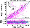 |
Fig. 1. Comparison of the hydrostatic mass estimates |


 (5)
(5)
We find a median fractional residual at R500,  , and its associated 1σ dispersion (16th–84th percentile range) to be equal to −0.24 ± 0.23. This corresponds to an average hydrostatic bias of (1 − b) = 0.75 ± 0.23, consistent with previous results by Ansarifard et al. (2020) and Gianfagna et al. (2023), both of which were also derived using data from THE THREE HUNDRED PROJECT. The scatter between the true mass and the hydrostatic mass is σscatter = 0.158 dex, reflecting the intrinsic variation beyond the mean bias.
To better understand the dispersion, we present in Fig. 2 the reconstructed pressure profiles obtained using local polynomial fitting for the 50 clusters with the lowest (left-panel) and highest (right-panel) mass bias, corresponding to the sets with the lowest and highest absolute value (modulus) of dispersion, respectively. These profiles are scaled by self-similar parameter  . For the least biased cluster set, the ratio between the true and reconstructed profiles remains very low, with deviations typically below 5% around R500. Similarly, the dispersion in the highest biased set increases beyond R500 but remains mostly below 10% around R500. The figures in the inset further reveal that the regular clusters predominantly belong to the relaxed category (χ < 0), whereas the outlier clusters are mainly disturbed objects (χ > 0). These results suggest that the large discrepancies in mass estimates for the outlier clusters can be attributed to their intrinsic dynamical state. Furthermore, in the central region and up to 0.6 R500, we find that the median pressure profile of the most biased set is approximately half that of the least biased set. This suggests that the highly biased clusters are predominantly composed of disturbed, non-cool-core systems, whereas the low-bias clusters are primarily relaxed cool-core clusters.
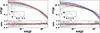 |
Fig. 2. Pressure profiles of clusters with low and high fractional dispersions in M500 derived using hydrostatic equilibrium. The grey lines show the pressure profiles of the 50 clusters having the lowest (left panel) and highest (right panel) fractional dispersions. The thick red lines indicate the corresponding median profiles. The bottom panel displays the ratio of reconstructed to true pressure profiles. In the right panel, we have also plotted the median profile for the lowest dispersion set with a thick blue line for comparison. The insets illustrates the distribution of the relaxation parameter χ for the same clusters. |
2.4. Training and testing samples
To enhance the dataset and improve model training, we augmented the sample by randomly placing simulated galaxy clusters at various redshifts within the range 0 ≤ z ≤ 1.2. For each placement, we recomputed the corresponding M500, accounting for its dependence on redshift through the critical density. Specifically, clusters originally at redshifts z = 0.07, 0.33 and 0.95 were randomly reassigned to the redshift bins [0.00 − 0.16], [0.16 − 0.65] and [0.65 − 1.2], respectively. These bins were chosen to preserve any potential redshift-dependent trends present in the original cluster samples, while allowing for variability within each bin. This approach enabled the same cluster to appear at different redshifts, thus incorporating redshift-dependent effects into the augmented sample. Furthermore, to explore the impact of radial coverage and binning – factors relevant to observational limitations (e.g. Chen et al. 2024) – we also modified the high-resolution simulated profiles, originally defined at 48 grid points across [0.02 − 2] R500. The number of radial bins was reduced (with a minimum of 7), and both the inner and outer radial boundaries were randomly varied to allow profiles of different radial ranges. The first radial bin was selected within [0.02 − 0.3] R500 and the last bin within [0.75 − 2] R500, resulting in a diverse set of profiles that more realistically reflect observational data quality. Importantly, care was taken to ensure that training and testing samples remained disjoint throughout the augmentation process. The original dataset was first divided into 1305 training and 350 testing clusters and each subset was then independently expanded to 9305 and 1950 clusters, respectively. Figure 3 shows the distribution of cluster masses across the different samples.
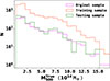 |
Fig. 3. Number distribution of galaxy clusters in the THE THREE HUNDRED PROJECT as a function of |

3. Graph neural networks
In this Section, we present an overview of Graph Neural Networks (GNNs). GNNs have already been applied to different astrophysical and cosmological studies (Makinen et al. 2022; Cranmer et al. 2021; Villanueva-Domingo et al. 2022; Jagvaral et al. 2022; Villanueva-Domingo & Villaescusa-Navarro 2022; Jespersen et al. 2022; Wu & Kragh Jespersen 2023; Lemos et al. 2023; Wu et al. 2024; Chuang et al. 2024). GNNs offer several advantages over CNNs, particularly when dealing with irregular data. While CNNs rely on predefined grid structures, GNNs can handle data of varying sizes and resolutions, making them well-suited for profiles or maps with different levels of granularity.
3.1. General concepts on graphs
A graph is represented as a combination of a set of nodes, V, and a set of edges, E, connecting these nodes: G = (V,E). In the context of GNNs, each node i ∈ V is characterised by a feature vector that encodes relevant information specific to that node. The edges (i,j) ∈ E indicate relationships between the nodes i and j. The structure of the graph is captured by an adjacency matrix A, where Aij = 1 if nodes i and j are connected by an edge, and Aij = 0 otherwise. The properties of the adjacency matrix depend on whether the graph is undirected or directed. In an undirected graph, the edge between nodes indicates a bidirectional connection, which results in a symmetric adjacency matrix Aij = Aji. In cases where there are no reciprocal directional relationships in the nodes, Aij is not symmetric. Since each node is connected exclusively to its neighbouring nodes, the neighbourhood of a node i, denoted  , consists of all nodes j that are directly connected to node i. Formally, this is expressed as
 (6)
(6)
3.2. Graphs from ICM profiles
In our approach, the radial profiles of the ICM are represented as graphs, where each node corresponds to a radial grid point, and the edges capture the physical relationships between neighbouring points, such as spatial proximity. Each node in the graph is assigned features representing the 3D physical properties of the ICM: temperature, density, pressure, total gas mass, and the corresponding radius. In this approach, xi represents the feature vector of the grid point i, where  contains the following five features: radius (Ri), density (ρi), temperature (Ti), pressure (Pi) and gas mass (Mg, i) as
 (7)
(7)
where R is in physical units and not in units of R500. Including derived pressure and gas mass as input features alongside the density and temperature could enhance the model’s robustness by providing additional physical context, allowing the neural network to learn relationships without predefined equations. For instance, the gas mass, as a cumulative property, will help to capture large scale spatial information, stabilising local variations and offering a global perspective on the ICM structure. We represent the complete set of feature vectors of all nodes of a given cluster as a matrix X, where  . Here, n represents the total number of nodes in the graph, which vary between 7 − 48, corresponding to the number of radial grid points and each row of the X corresponds to the feature vector of a specific node, thereby capturing the physical properties of the ICM across the entire grid. The set of edges E is constructed based on the spatial relationships between grid points. Specifically, in our model, each node i is assumed to be connected with every other node j4. Furthermore, nodes are assumed to be connected symmetrically, so the adjacency matrix satisfies, Aij = Aji, enabling bidirectional information flow. The graph-based representations are then processed by the GNN described in the following subsections.
3.3. Message passing in GNNs
Unlike traditional neural networks, which are tailored for structured data such as images (grids) or sequences (ordered tokens), GNNs are designed to handle graph-structured data, where the underlying topology can be irregular and non-Euclidean. The key operations in GNNs are neighbourhood aggregation and feature update, where a node’s feature vector is aggregated from the features of its neighbouring nodes and then updated through a learnable transformation. The forward propagation in a GNN layer can be generally described using the message-passing framework as
 (8)
(8)
where hv(k) is node v’s feature vector at layer k and 𝒩(v) denotes its neighbours. The message function ψ computes interactions between nodes, ⨁ aggregates neighbour messages (using sum, mean, max, or attention), and ϕ updates the node state (typically a neural network with non-linearity).
For instance, Graph Convolutional Networks (GCNs) (Kipf & Welling 2016) update the node features using a sum of normalised neighbourhood embeddings, by combining each node’s feature with those of its neighbours after normalising them by their degrees, and thus effectively applying convolutional filters on the graph. Graph Attention Networks (GATs) (Veličković et al. 2017), on the other hand, employ attention mechanisms to assign varying weights to neighbouring nodes, capturing their differing influences through learnable attention coefficients. While GCN or GAT typically operate in a transductive setting – learning node embeddings based on the fixed graph structure seen during training – GraphSAGE networks (Hamilton et al. 2017) introduces an explicitly inductive approach by learning parameterised aggregation functions (e.g. mean, LSTM, pooling) that can be applied to the features of sampled neighbours, allowing it to generate embeddings for unseen nodes or entirely new graphs at inference time. Similarly, Graph Transformer networks (Shi et al. 2020) extend the inductive capabilities by incorporating multi-head self-attention mechanisms over a node neighbours, enabling more expressive and flexible neighbourhood aggregation that can generalise to unseen nodes or graphs. Another approach is that of the Gated Graph Neural Networks (GGNNs) (Li et al. 2015) that incorporate recurrent units such as Gated Recurrent Units (GRUs) to iteratively update the node states, enabling the capture of more complex and long-term dependencies within the graph. Each of these models showcases a different strategy for refining the node representations based on their neighbourhood information, enabling GNNs to extract intricate patterns from graph-structured data.
3.4. Model architecture
We implement our graph neural network (GNN) architecture using the PyTorch Geometric library, which provides a wide range of message-passing layers. We consider several types of of message-passing layers: Graph Convolutional Network (GCNConv), Graph Attention Network (GATConv), GraphSAGE (SAGEConv), and Graph Transformer (TransformerConv). As discussed in the previous Section, these layers enable the network to aggregate information from neighbouring nodes based on different mechanisms, allowing it to capture both local and global structural patterns within the graph. In the current implementation, we do not use multi-head attention for the Transformer GNN; the layer is applied with a single attention head to maintain a fixed embedding size and simplicity.
Following the message-passing layers, we apply one of several global pooling operations to aggregate the node-level features into a fixed-size graph-level representation. Specifically, we consider global mean pooling, global sum pooling, global max pooling and an attention-based pooling strategy. In the attention-based variant, learnable attention weights are used to highlight the most informative nodes during the pooling operation. Specifically, a linear layer computes a score for each node, which is then normalised and used to weight the node features during aggregation, allowing the network to focus on key nodes that contribute most to the overall graph representation.
The first message-passing layer receives node features of size 5, which correspond to the temperature, density, pressure, gas mass of the ICM, and the radius associated with each node. These features are projected into a higher-dimensional embedding space. Subsequent message-passing layers refine these embeddings while maintaining the same dimensionality, enabling the network to learn rich, hierarchical representations of the graph. Each layer is followed by batch normalisation and a ReLU activation function to stabilise training and introduce non-linearity, improving the model’s capacity to capture complex relationships between node features.
To incorporate external redshift information, we concatenate the redshift value to the pooled graph embedding, forming a combined representation that captures both structural and redshift-dependent information. This combined embedding is then passed through a series of fully connected linear layers. These layers are followed by batch normalisation and ReLU activation. The final linear layer outputs a single scalar prediction, representing the cluster mass M500, which is the target variable of the model.
3.5. Model training
Before training the model with the sample described in Sect. 2.4, we first normalised the pressure, gas mass, radius, and total mass respectively by 10−10 erg cm−3, 1014 M⊙, 103 kpc, and 1015 M⊙, so that their maximum value is close to unity. The ICM density (in cm−3) and temperature (in KeV) profiles were not normalised since their values are already within a manageable scale and do not present issues of large magnitude that could destabilise gradient descent during training. Thereafter, all quantities were transformed to base-10 logarithmic space to further stabilise the training and better capture multiplicative relationships between variables. We employed the mean absolute error (MAE) as a loss function, defined as
 (9)
(9)
where  and
and  are the true and predicted values of 3D M500 for the galaxy cluster l, and N is the number of clusters in the sample (training or testing set).
The optimal values of hyper-parameters discussed in the next paragraph were obtained using Optuna5 (Akiba et al. 2019), which efficiently searches for the best combinations by minimising the average test loss utilising the Tree-structured Parzen Estimator (Watanabe 2023).
The Adam optimiser was used with an initial learning rate of 9.9 × 10⁻⁴ and weight decay set to 2 × 10⁻³ to mitigate overfitting. We used the ReduceLROnPlateau scheduler, which adaptively lowers the learning rate when validation loss plateaus to improve convergence. The reduction scale was controlled by the lr factor of 0.5, with smaller values enabling finer adjustments. The training set was divided into a batch size of 128 graphs. Gradients were calculated through backpropagation, and the optimiser updates the model parameters. After each epoch, the model was evaluated on the training and testing sets to assess performance. At round 500 iterations, we find the value of the loss function is well flattened, indicating minimal further improvement. At this point, we considered the training to have sufficiently converged and stopped the process. We used three TransformerConv layers with an embedding size of 128 along with global max pooling. The graph-level embedding was followed by three fully connected linear layers: the first reduced the dimensionality from 129 to 60, the second from 60 to 30, and the final output layer produced a scalar prediction.
Table B.1 in Appendix B lists the hyper-parameters used in this work. Table B.2 in Appendix B presents a comprehensive overview of our GNN architecture, detailing the type, input size, output size, and function of each layer.
To account for the effects of random initialisation, we trained a total of 50 individual models, each initialised with different random weights. By aggregating the predictions from these models, we aim to mitigate the risk of any specific initialisation, thereby improving the overall robustness and generalisation capability of our ensemble. Each model was weighted according to its validation loss, allowing us to give greater importance to models that perform better. The final predicted mass, given the input X, is defined by the weighted mean over the ensemble. The final loss values showed minimal variation across different models. In Fig. 4, we plot the training and testing losses for one of the models. The gradual decline in both losses indicates stable learning, converging to final values.
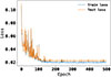 |
Fig. 4. Train and test loss in the evaluation mode over epochs for one of the ensemble models. Both train and test losses indicate consistent learning, with the final loss at around 0.02 for the training and testing sets. |
4. Model evaluation
In this Section, we evaluate the performance of our model in predicting galaxy cluster masses, specifically the characteristic mass M500. We examine the model’s robustness to observational constraints, analyse its sensitivity to cluster dynamical states, and compare its performance to the traditional hydrostatic mass estimation method. Finally, we use interpretability tools to understand the contributions of various radial thermal profile features to the model’s predictions.
4.1. Performance of the GNN model
To evaluate the generalisability of our GNN model, we tested it on a reserved dataset spanning radial profiles which have an extent up to [0.75–2] R500. This dataset covers an extensive range of ICM properties across radii, allowing us to rigorously assess the model’s capacity to perform accurately on unseen data. Figure 5 displays the distribution of GNN predicted masses,  , versus true cluster masses,
  , for both the testing (right panel) and training (left panel) samples, illustrating the model’s ability to align its predictions closely with true values. This strong alignment confirms that the GNN effectively captures the patterns of the mass distribution across various scales, demonstrating robust generalisability beyond the training set. In particular, we observe that the median fractional residuals,
  , remain near zero throughout the mass range. We find the fractional residual to be 0.00 ± 0.06 and 0.00 ± 0.05 for the testing and training samples, respectively. Similarly, the mass bias, (1 − b), is equal to 1.00 ± 0.06 for the testing sample and 1.00 ± 0.05 for the training sample. Finally, we find the scatter between the true and predicted mass to be 0.026 dex and 0.023 dex for testing and testing samples, respectively. In terms of mass estimation accuracy, the model achieves an R2 score of 0.99 on both testing and training samples, reflecting its high fidelity in reproducing true masses with minimal error. This level of accuracy suggests that the GNN can reliably estimate masses across diverse radial profiles, underlining its potential for applications requiring accurate mass distribution predictions.
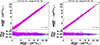 |
Fig. 5. Distribution of GNN predicted masses, |


To our knowledge, this is the first model to attain lower than 7% scatter using only low-dimensional spherically symmetric radial profiles as input, providing a robust and efficient alternative to image-based methods. Green et al. (2019) employed ensemble regressors on morphological features extracted from simulated X-ray maps and reported a mass scatter of ∼16%. Similarly, Ntampaka et al. (2019) and Yan et al. (2020) achieved scatters of ∼12% and ∼16%, respectively, using neural networks trained on Chandra-like mocks generated from simulations. On the other hand, de Andres et al. (2022) demonstrated that CNN-based estimators using SZ observations can achieve ∼10% scatter which is comparable to the accuracy achieved in our work using X-ray data. Krippendorf et al. (2024) applied CNNs to multi-band eROSITA mocks and reported a scatter of ∼19%, meanwhile, Ho et al. (2023) using similar architecture achieved a best-case scatter of about 16%. Despite using richer, higher-dimensional inputs, both studies report higher scatter than our GNN model trained solely on single-band radial profiles, which attains substantially lower scatter by utilising lower-dimensional physically interpretable features.
While direct, one-to-one comparisons between these studies remain inherently difficult due to differences in simulation suites, input representations, model architectures, training objectives, and sample selection, our comparisons should be viewed as indicative rather than definitive. A standardised benchmark using consistent simulation and observation pipelines will be crucial for a robust comparison of future machine learning-based mass estimators and will be performed in the future studies.
To assess the impact of core regions on mass estimation, we also trained a GNN model on core-excised profiles, as discussed in Appendix C. By excluding the AGN-dominated central ICM (within ∼0.1, R500), we observe a slight improvement in the scatter of predicted masses (0.025 dex in testing sample). In Appendix D, we trained two additional variants of our fiducial model. The first variant used only three features – radius, density, and temperature – while the second included six features, incorporating entropy in addition to those used in the fiducial model. For the three feature model, the bias and fractional residuals are unbiased, but the scatter in the testing sample is about 1.5 times larger than for the fiducial model. For the six-feature model, we observe no reduction in scatter compared to our fiducial model. Moreover, the inclusion of entropy as a feature does not necessarily translate to more physically robust predictions. From an observational standpoint, entropy measurements are known to be significantly affected by gas clumping, which can introduce systematic uncertainties.
Similarly, in Appendix E, we investigated the impact of a redshift dependence on model training by using distinct redshift bins for the training and testing samples. We find that when the model is trained on low-redshift (z = 0.06) and intermediate-redshift (z = 0.33) samples – both augmented within the redshift range 0 ≤ z ≤ 1.2 (with random binning sizes as done for the main case) – and then tested on a high-redshift sample at z = 0.96 (also augmented over the same redshift range and binning). We find that the fractional dispersion for the testing sample has a median of −0.04 ± 0.07, with a median bias of 0.96 ± 0.08 and a scatter of 0.061 dex. In contrast, for the training sample, the fractional dispersion and bias are 0.00 ± 0.05 and 1.00 ± 0.06, respectively, with a scatter of 0.025 dex. The larger dispersion and bias on the testing sample compared to the training sample suggest that the model may be overfitting to the lower-redshift training data. This comparison illustrates that the redshift distribution of the training data plays an important role. In particular, the underrepresentation of high-z clusters in the training set limits the model’s ability to capture the evolving thermodynamic and structural properties of the ICM, leading to a mild systematic bias and increased scatter in the predictions.
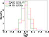 |
Fig. 6. Histogram of residual distributions for the entire unaugmented test sample of 350 galaxy clusters, and for the 50 most relaxed and 50 most disturbed clusters within this sample. The vertical dashed lines show the corresponding median of distributions. We find comparable performance of the GNN model across different dynamical states. |
4.2. Impact of cluster dynamical state on model performance
To assess how the dynamical state influences the model performance, we evaluated the GNN separately on relaxed and disturbed clusters in the original, unaugmented testing sample of 350 clusters. Figure presents the histogram of residual distributions for the entire unaugmented test sample, as well as for the 50 most relaxed and 50 most disturbed clusters within this sample. Our results indicate that the residuals are comparable across these subsamples. Across the test set, the median residuals (with 1σ dispersions) are 0.00 ± 0.05 (scatter 0.023 dex), 0.02 ± 0.05 (scatter 0.017 dex) and −0.01 ± 0.04 (scatter 0.023 dex) for the unaugmented high-resolution test sample of 350 clusters, the 50 most relaxed clusters and the 50 most disturbed clusters, respectively. In all cases, the scatter is less than 7%, demonstrating that the GNN model maintains consistent performance for both relaxed and disturbed morphologies.
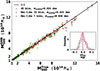 |
Fig. 7. Comparison of predicted and true galaxy cluster masses for an unaugmented test sample of 350 clusters. The black line represents a 1-to-1 relation. The magenta, orange, and green points represent predictions using ICM profiles truncated respectively at 2R500, R500, and 0.75 R500, with 48, 15, and 7 bins. The inset shows the corresponding fractional residuals; the vertical lines represent the medians. |
4.3. Performance with respect to observational-like profiles
To simulate observational constraints, we truncated the ICM profiles to R500 and 0.75 R500, assigning 15 and 7 observational bins, respectively. These truncations mimic the radial limits of current X-ray observations, approximating the depth of XMM-Newton’s deep and shallow observations. This approach tests the GNN’s robustness when spatial information is limited. Despite the reduced radial coverage, the GNN achieves a robust mass estimation accuracy with a precision of better than 10% on average, with respect to the true mass. Figure compares predicted and true cluster masses in the observational-like profile datasets, using the original testing sample of 350 galaxy clusters. The model captures the overall mass distribution well, even with restricted radial data. The median fractional residual error and the associated 1σ dispersion are consistent with zero, with values of 0.00 ± 0.05 (scatter 0.024 dex), 0.01 ± 0.06 (scatter 0.025 dex) and 0.00 ± 0.08 (scatter 0.036 dex) for the 48 (fine bining), 15 bin and 7 bin cases, respectively. These results highlight the model’s adaptability to incomplete data while maintaining strong predictive performance. In Table 1, we give the best-fit linear relation between the GNN derived masses versus true masses. Finally, we tested a model in which the central region (< 0.1 R500) of the input profiles was excluded from the mass estimation using our fiducial model. The model performance remains very similar across all three cases – fine binning and coarse binning with 15 and 7 bins – with scatters of 0.024, 0.025 and 0.027 dex, respectively. This performance is similar to the results obtained with the core-excised model where the model was trained with input profiles having radii > 0.1 R500. This reaffirms that feedback processes, which dominate in the central region, diminish its constraining power, thereby limiting the impact of its exclusion on the model’s accuracy.
4.4. Model variance estimation
To quantify model (epistemic) uncertainty in the inference of cluster masses, we adopt a simulation-based inference (SBI) framework Kodi Ramanah et al. (2021). Following the approach of de Andres et al. (2022), we employ a kernel density estimation (KDE)-based SBI method in which the posterior distribution over the true cluster mass θ (i.e.  ) is inferred from the predicted mass
  (i.e.
(i.e.  ) via a trained ensemble of GNNs. From the training set, we collect pairs of predicted and true masses
  , and use them to estimate the joint distribution
  via a two-dimensional Gaussian KDE.
For a test sample with GNN predicted mass  , we obtain the conditional posterior
  by evaluating and normalising the joint distribution at
  . The posterior mean (θpost) and variance (σ2) are then given by
 (10)
(10)
This non-parametric approach avoids explicit likelihood modelling and enables flexible posterior estimation over cluster masses, grounded in the relationship between GNN predictions and true target values.
Figure 8 shows the predicted model uncertainty σGNN versus the true cluster mass  for the test sample. We observe a clear trend of increasing uncertainty with increasing mass, suggesting that the model is less confident in its predictions for higher-mass clusters. This may be attributed to limited training examples at the high-mass end, or to more complex feature–target relationships in massive systems. However, the fractional percentage errors remain approximately 5% for most clusters, increasing to about 10% for clusters with masses below 2 × 10^{14} M⊙. The plot in the inset shows that posterior means closely match the GNN point estimates, indicating that the model is well-calibrated and that its predictions lie in regions of the input space well-supported by the training set. In later Sections, where observed data with errors are considered, we also incorporate aleatoric (data) uncertainty by performing Monte Carlo simulations to propagate these uncertainties through the model.
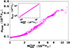 |
Fig. 8. 1σ GNN model uncertainty, σGNN, estimated using KDE-based SBI, as a function of the true cluster mass |

Finally, we note that probabilistic neural networks (e.g. evidential and Bayesian neural networks) were not employed in this work. First, these models often require strong parametric assumptions regarding the uncertainty structure and prior distributions. Second, our training sample is relatively small, particularly in the high-mass regime, which may hinder the precise estimation of model variance. Nonetheless, we plan to implement a full Bayesian formalism in future work with larger training datasets.
4.5. Model extrapolation ability
To evaluate the extrapolation capabilities of our GNN model trained on ICM graph data spanning the radial range from 0.75 R500 to 2 R500, we conducted additional checks using ICM profiles restricted to smaller inner radial ranges using unagumented testing sample of 350 galaxy clusters. Specifically, we tested the model’s performance when provided with data only up to 0.5 R500 (case A), 0.4 R500 (case B) and 0.3 R500 (case C) with 7, 5 and 5 bins respectively. Figure 9 summarises the model predictions, while Table 2 reports the best-fit linear relations between predicted and true masses for these cases. The median fractional residuals are 0.00 ± 0.13, 0.01 ± 0.18 and 0.06 ± 0.25 for cases A, B, and C, respectively. We observe an increasing scatter and a progressive bias in the recovered masses as the radial range decreases, indicating that the model’s performance degrades when extrapolating to the inner regions not covered during training.
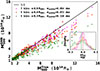 |
Fig. 9. Extrapolation performance of the GNN model when evaluated with input data restricted to the inner regions. The plot shows predicted vs. true cluster masses for three cases where the available ICM data extends only up to 0.5 R500, 0.4 R500, and 0.3 R500, corresponding to Case A, B, and C in the text and 7, 5, and 5 radial bins, respectively. |
4.6. Comparison to traditional hydrostatic masses
The hydrostatic method, which assumes equilibrium within the ICM, typically relies on density and temperature (or pressure) measurements at a specific radius, R, to estimate the cluster mass within that radius. This approach, therefore, emphasises local indicators of mass, assuming a smooth, stable distribution of gas within the cluster. However, this assumption may not hold in clusters that have undergone significant dynamical interactions and in galaxy cluster groups, which may experience strong AGN-driven outflows to larger radii, leading to inaccuracies and increased scatter in mass estimates.
In contrast, the GNN model is more expansive, using both core and outer radial features in its mass predictions. The graph-based approach allows the GNN to capture the complex, non-local dependencies between different regions of the cluster, making it more robust to dynamical processes that can disrupt the ICM equilibrium. This capability allows the GNN to better capture the intricate dynamics of disturbed clusters, adapting to varying physical conditions. As shown in Fig. 10, the scatter in M500 estimates, in the unaugmented test sample, is larger for the hydrostatic method compared to the GNN model. We find that for the unaugmented test sample of 350 galaxy clusters, the median fractional dispersion in M500 is biased by −0.27 ± 0.21 and has a scatter that is about six times larger than that for the GNN-derived results.
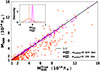 |
Fig. 10. Comparison of GNN and hydrostatic equation predictions for M500 using an unaugmented test sample of 350 galaxy clusters. The black line represents a 1-to-1 relation. The magenta and orange points respectively compare the GNN predictions and the hydrostatic predictions with the true masses. The inset shows the distribution of residuals for both approaches; the vertical lines show the median of the distributions. |
4.7. Model interpretability: feature importance analysis
We use integrated gradients to identify which features contribute most to the GNN mass predictions. This approach helps understand model behaviour in complex astrophysical data, where feature contributions are not always clear. Integrated gradients calculate the gradients of the loss function with respect to each input feature by interpolating between a baseline (average feature profile) and the actual inputs. These gradients are tracked and averaged across batches, providing a measure of feature importance. Higher values indicate features that are more important for predicting galaxy cluster mass.
Figure 11 presents the feature importance for each input quantity in determining the total mass of galaxy clusters. The relative importance values are [R, ρ, T, P, Mg] = [0.29, 0.20, 0.06, 0.10, 0.34], highlighting that the model places the greatest emphasis on the integrated gas mass and radius features. This outcome is physically motivated: the gas mass profile, being a cumulative quantity, is a direct tracer of the gravitational potential. Moreover, since the gas mass is derived from the integral of the gas density profile, it effectively encodes information regarding both the density normalisation and slope, which are key to determining the total mass distribution. The radius defines the spatial scale over which all other quantities (e.g. density, temperature) are evaluated, thus implicitly contributing to how gradients are computed.
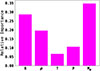 |
Fig. 11. Average feature importance for predicting M500 as a function of input features. Shown are the relative importance of the five features, i.e. density (ρ), temperature (T), pressure (P), gas mass (Mg), and radius (R). |
To test the relative importance of these features, we trained a model using only the radius and gas mass as inputs. Remarkably, the model performance showed a negligible decrease compared to when using the set of thermodynamic profiles used for the fiducial five feature model with dispersion and scatter of 0.00 ± 0.07 and 0.030 dex, respectively. This result supports the physical interpretation with the integrated gradients analysis. However, its extrapolation capability is significantly compromised. When applied to clusters with limited radial coverage – as in the extrapolation tests described previously – the model performance, already poor in the fiducial case, deteriorates even further with scatter equal to 0.065, 0.090 and 0.130 dexs for the cases A, B and C, respectively. This suggests that the additional thermodynamic features, though not critical for performance within the training range, provide contextual information that is important for reliable generalisation beyond it.
In contrast, density, temperature, and pressure features – while central to understanding the thermodynamic state of the ICM – do not provide as direct a constraint on the cluster mass if gas mass is taken into account. Their local values are sensitive to small scale fluctuations or non-thermal processes, making them less important predictors compared to gas mass. Therefore, the model naturally learns to prioritise integrative or structurally representative features – Mg and R – which carry global information about the cluster mass distribution. However, as seen in Appendix D, if the gas mass feature is ignored and the model is trained with the feature set consisting of radius, density, and temperature only, then density and radius become crucial, albeit with a larger scatter, i.e. 0.038 dex for the testing sample.
5. Application to observed data
In this section, we apply the GNN model to galaxy cluster data obtained from XMM-Newton X-ray observations. The X-ray observations that we used, and describe below, provide all the features required by the GNN model, including the deprojected (3D) profiles that we have tested in the previous Sections. This comparison provides insights into the potential improvements from machine learning models like GNN, and the need for corrections in mass scaling relations.
The SZ cluster mass, M , is derived from the SZ effect, which measures the interaction of high-energy electrons in the ICM with the CMB photons. This interaction distorts the CMB spectrum, with the SZ observable,
  , representing the volume-integrated pressure of the ICM. The SZ effect, being independent of redshift, provides a direct and robust probe of cluster properties across cosmic epochs. The SZ scaling relation is established by calibrating these SZ and X-ray observables against hydrostatic mass estimates, MHSE, derived from detailed modelling of pressure and density profiles (Arnaud et al. 2010). Such scaling relations are indispensable for cluster-based cosmological studies, enabling robust constraints on dark energy and structure formation. For cluster cosmology using the Planck SZ derived masses as reference cluster masses (Planck Collaboration Int. III 2013), it has been demonstrated that the SZ and X-ray derived masses are generally consistent within expected uncertainties (Planck Collaboration Int. V 2013)6. In Appendix F and Appendix G, we also compare the X-ray derived masses with the GNN masses.
For our analysis, we consider two well-known cluster samples. We first consider the REXCESS (Representative XMM-Newton Cluster Structure Survey) sample, which consists of a carefully selected set of 31 galaxy clusters from the REFLEX catalogue, having redshifts between z = 0.055 and 0.183. These clusters were chosen to provide a statistically representative view of cluster properties across a range of masses and morphologies. Using high-quality X-ray observations from XMM-Newton has resulted in in-depth analysis of the ICM in these clusters (Böhringer et al. 2007; Croston et al. 2008; Pratt et al. 2007, 2010; Arnaud et al. 2010). This analysis includes deriving radial profiles of density, temperature, and entropy, which are crucial for understanding the thermodynamic state and structural characteristics of the clusters. Studying these profiles and establishing scaling relations, such as those between X-ray luminosity and temperature, has led to valuable insights into the physics governing galaxy clusters and aids in cosmological studies that use clusters as probes of large-scale structure and cosmic evolution. In our previous work, we used this sample to study the non-gravitational feedback in galaxy clusters (Iqbal et al. 2018).
We also consider the X-COP (XMM-Newton Cluster Outskirts Project) sample which is an X-ray (XMM-Newton) follow-up project of a Planck SZ-selected set of 12 galaxy clusters in the redshift range of 0.04 < z< 0.1, chosen to facilitate a detailed study of cluster properties extending into their outer regions (Eckert et al. 2017). The selection criteria leverage the SZ effect’s sensitivity to gas pressure and the X-ray emission’s dependence on gas density, enabling comprehensive measurements of density, pressure, temperature, and entropy profiles from the cluster core to the outskirts (Ghirardini et al. 2019; Eckert et al. 2019). The X-COP sample’s findings contribute to a better understanding of galaxy cluster formation, as well as refining cluster-based cosmological constraints by reducing biases associated with mass estimates (Eckert et al. 2019, 2022). In particular, Eckert et al. (2019) not only estimated the hydrostatic mass but also proposed a method to estimate the total mass, which includes the contribution from non-thermal pressure using hydrodynamical simulations (Nelson et al. 2014).
5.1. Estimation of GNN masses (M )
)
We use the ICM profiles of the REXCESS sample derived in Böhringer et al. (2007), Croston et al. (2008), Pratt et al. (2010), Arnaud et al. (2010) to estimate M500 using the GNN model. Similarly, for the X-COP sample, thermal profiles derived in Ghirardini et al. (2019) were used to estimate GNN masses. As the GNN model output is predominantly influenced by the gas mass, we employ density-defined radial annuli at the node points and interpolate the temperature profile to estimate its values at these nodes. However, only the nodes whose radii fall within the observed range of the temperature profile are taken into account. Moreover, the innermost 50 kpc of the profiles were excluded, since this region is dominated by feedback processes. To obtain an estimate of the uncertainty in the GNN masses, we simulated 100 observed ICM profiles by assuming log-normal distribution for density and temperature profiles (Kawahara et al. 2007), with the standard deviation taken as the observed uncertainties. For each cluster, we computed GNN derived mass, M , as the mean output of these 100 simulations. Two contributions to the total uncertainty were then considered. The first is the variance of the predicted masses across the 100 realisations, which reflects the sensitivity of the GNN predictions to observational uncertainties in the input profiles. The second is the mean of the SBI predicted variances from the GNN model for each realisation, which represents the intrinsic uncertainty of the model predictions. Tables F.1 and G.1 in Appendices F and G provides the GNN mass for the REXCESS and X-COP samples, respectively, along with other mass proxies. We emphasise that the uncertainties in the GNN derived cluster masses are primarily driven by model variance, rather than by the observational uncertainties of the input X-ray profiles.
5.2. Estimation of SZ masses (M )
)
Out of the 31 clusters in the REXCESS sample, 23 are included in the PSZ2 cluster catalogue (Planck Collaboration XXVII 2016), meaning the rest are below the PSZ2 catalogue detection threshold corresponding to a signal-to-noise of 4.5. We thus lacked published SZ mass estimates for a large fraction of the sample. To overcome this problem, we performed a targeted, unblind extraction of the REXCESS sample in the Planck data, fixing the position to that of the REXCESS catalogue. We also performed the same extraction for the twelve X-COP clusters to obtain fully homogeneous SZ mass estimates of the REXCESS + X-COP sample.
In practice, we worked with the six all-sky maps of the High Frequency Instrument of Planck (Planck Collaboration VIII 2016). We used the MMF3 algorithm based on multi-frequency matched filters developed for the Planck analysis (Melin et al. 2006, 2012). The MMF3 algorithm produces cutouts (10 × 10 deg2) of the Planck maps centered on each cluster and combines them optimally to extract the cluster flux. The algorithm assumes a fixed spatial profile for the SZ signal, specifically, the universal pressure profile of Arnaud et al. (2010) while leaving the amplitude as a free parameter. The SZ spectral dependence was also modelled using the non-relativistic limit. The MMF3 algorithm scans over a grid of 32 logarithmically spaced θ5007 from 0.94 to 35.32 arcmin. For each cluster, we extracted its SZ flux Y500 as a function of the size θ500 and the associated signal-to-noise ratio S/N. Following the method described in Sect. 7.2.2 of Planck Collaboration XXIX (2014), we broke the Planck flux–size degeneracy by applying an X-ray prior based on the scaling relation given in Eq. (5) of Planck Collaboration XXIX (2014), which links the SZ flux to the cluster size, assuming the redshift is known. This allowed us to derive the Planck flux and, subsequently, the SZ mass M of the cluster. The corresponding 68% confidence intervals on the flux were estimated using the same approach, by calculating
  . We were able to extract homogeneous flux and masses for all the clusters but one, RXC J1236.7–3354, from REXCESS, whose signal to noise was S/N = 0.2, resulting in a measured flux consistent with zero.
5.3. Comparison of SZ masses with GNN masses
To analyse the comparison between masses derived from the GNN model and those obtained from the SZ scaling relation, we can focus on the bias and the fractional residuals as key metrics. Figure 12 shows the comparison of GNN masses to the SZ masses and the relative bias (M /M
/M ) for the combined REXCESS and X-COP sample. Assuming M
 to be the ‘true’ unbiased cluster masses, we find a bias (1 − b) and fractional residuals of
  and
and  respectively for M
 masses. However, if we only consider the X-COP sample we find the bias and fractional residuals to be
  and
and  respectively. The significantly tighter constraints observed in the X-COP sample could be attributed to its better data quality and to the sample’s extended coverage into the cluster outskirts. In contrast, the REXCESS sample comprises relatively low-mass clusters, as seen in Fig. 12, and tends to exhibit smaller mass biases; in fact, a bias of > 1 is observed for many low-mass clusters. This contributes to the broader dispersion observed in the combined sample. We find the best-fitting linear relation for the combined sample by employing the Gaussian mixture model LinMix (Kelly 2007)
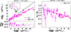 |
Fig. 12. Left panel: Comparison of masses derived from the GNN model with those obtained from the SZ scaling relation. The black line represents the ideal 1-to-1 relation. The inset shows the distribution of fractional residuals. The right panel shows the bias in the SZ determined mass (M |


 (11)
(11)
In particular, if the intercept is fixed to zero, we find a best-fitting slope (bias) to be 0.81 ± 0.02.
The right panel of Fig. 12 shows the relation between the bias and cluster mass. We quantify the bias-mass relationship by the following power-law fit
 (12)
(12)
This relation reveals a strong trend, at 5σ significance, of decreasing 1 − b (i.e. increasing bias) with increasing cluster mass, indicating that more massive clusters exhibit stronger biases in SZ derived masses. This trend is physically consistent with the expectation that non-thermal pressure support arising from bulk motions, turbulence, and ongoing merger activity becomes increasingly important in massive systems.
de Andres et al. (2022) also found that less massive clusters exhibit a smaller bias when comparing Planck masses to those estimated with a deep learning technique using the THE THREE HUNDRED PROJECT simulation. They further argued that the derived bias could be potentially explained due to differences in the slopes of Y-M scaling relations between the observations and THE THREE HUNDRED PROJECT simulations. This explanation aligns with the positive bias found in some of the low-mass clusters in our work.
A comprehensive assessment that incorporates additional non-SZ mass proxies – such as weak lensing, galaxy dynamics, or refined hydrostatic mass estimates which incorporate no-thermal pressure – would provide a more robust cross-validation of our results. Each of these methods probes different physical aspects of the cluster potential: weak lensing directly traces the total matter distribution without assumptions about the dynamical state, galaxy dynamics capture the kinematic imprint of the gravitational potential, and hydrostatic masses constrain the thermodynamic equilibrium of the ICM. By jointly considering these complementary techniques, one could better quantify systematic uncertainties (e.g. non-thermal pressure support, line-of-sight projection effects, or sample selection biases) and isolate potential deviations from the self-similar scaling expectations. However, such an analysis requires careful homogenisation of datasets and treatment of selection effects, which is beyond the scope of the present work. We therefore defer this more detailed, multi-probe study to future work.
6. Discussion and conclusions
Hydrodynamical simulations of galaxy clusters are essential for interpreting X-ray observations as they model the complex distribution and behaviour of the hot and diffuse ICM. These simulations enable the prediction and comparison of projected quantities such as temperature, density, pressure, and entropy profiles, which are critical for analysing the physical conditions within clusters. By matching these projections to the observed X-ray data, we can gain insights into key processes, such as gas cooling, shock heating, turbulence, and feedback from AGN. Recent advances in hydrodynamical simulations have led to increasingly realistic models that closely match observations in both large-scale structures and finer intra-cluster features (Cui et al. 2018; Braspenning et al. 2024; Lehle et al. 2024; Riva et al. 2024). On the other hand, deep learning techniques have become increasingly important for revealing complex non-linearities in astrophysical data. While traditional methods may struggle to capture the intricate relationships between different physical quantities, especially when dealing with large noisy observations or when attempting to model highly non-linear processes, deep learning models have shown great promise in learning these complex relationships directly from observational data without relying heavily on pre-defined physical assumptions (Alzubaidi et al. 2021).
Departing from traditional methods that rely on the hydrostatic equilibrium assumption, our approach incorporates high-resolution thermal profiles of the ICM and total dark matter profiles from hydrodynamical simulations and a deep-learning approach to uncover the intricate nature of the ICM and cluster mass (M500) relationship using X-ray observations, implicitly accommodating the effects of non-thermal pressure components. While the estimates of integrated mass, M(< R), at a given radius, R, in the hydrostatic framework rely heavily on data around R and are sensitive to noisy derivatives, our approach learns the overall structure of the data to yield robust estimates of M500. We find that, in general, our GNN model can accurately recover M500. We summarise our results and the performance of the GNN model in estimating the mass of galaxy clusters as follows:
-
The performance of the trained GNN model is consistent across the training sets and the testing sets, with a bias in M500 equal to zero and a median fractional dispersion of around 6% within the mass range 1 × 10¹⁴ M⊙ ≤ M500 ≤ 2 × 10¹⁵ M⊙. Additionally, our model outperforms classical hydrostatic modelling, which shows a bias of approximately 20% as well as scatter that is about six times larger than that of our GNN-based approach.
-
We evaluated the GNN performance on the most relaxed and disturbed clusters in the test sample to understand how the cluster dynamical state affects model adaptability. The GNN achieves consistent adaptability across these morphological states, with comparable error distributions between relaxed and disturbed clusters. This suggests that the model effectively captures key structural features of the ICM, maintaining stable performance despite variations in cluster dynamical states.
-
We tested the model using observational binning, truncating the profiles at R500 and 0.75 R500 (15 and 7 bins). Despite the reduced radial coverage, the GNN estimates cluster masses with high accuracy, yielding scatter of 5.6%, 5.9%, and 9.1% for the 48, 15, and 7 bin cases, respectively. Moreover, if the core input profiles are excluded (< 0.1R500), the scatter in the seven-bin case is reduced to 6.4%
-
We used integrated gradients to reveal which features most influence the GNN’s mass predictions. We find that ICM gas mass and radius are the most influential features, as they directly correlate (increasing profiles) with the galaxy cluster’s mass. Other features, such as temperature and pressure, play supporting roles but have a less direct impact on mass prediction.
-
We applied the GNN model to the joint REXCESS and X-COP X-ray sample. Our findings indicate a strong mass dependent bias, at 5σ confidence, with high-mass clusters exhibiting a greater degree of bias.
-
The significant detection of a mass-dependent bias could introduce a crucial refinement to the use of galaxy clusters as cosmological probes. Such a trend implies that high-mass clusters typically used as anchors in cosmological analyses may be more strongly biased, potentially leading to a reduction in the tension in σ8 between the CMB cosmology and SZ cluster counts.
Our results align with recent neural network models developed in de Andres et al. (2022), Ferragamo et al. (2023), de Andres et al. (2024), which successfully learn the connections between observed maps and total mass maps or profiles, thus providing unbiased estimates of total mass. However, the GNN approach introduced in this work significantly diverges from these methodologies. While the studies mentioned rely on fixed-grid image-based deep learning techniques such as CNNs and U-Net to estimate mass proxies or project total mass density maps from multi-wavelength hydrodynamic simulations having a fixed grid (with de Andres et al. 2022 exclusively using SZ maps to estimate M500), the GNN model processes 3D deprojected radial profiles of the intracluster medium obtained in X-rays. This is achieved by learning the spatial and hierarchical structure of data encoded as a graph. Although the GNN approach assumes a simplified spherical symmetry and uses 3D profiles that are not directly observable, it achieves better accuracy while offering the flexibility to handle input data of varying sizes.
Our models used 3D profiles from simulations and are tested on deprojected profiles from observations. Potentially, one could use 2D features, i.e. the projected observational profiles. However, this would require training separate models, which we aim to explore in the future, even extending the work to different instruments, thus changing the response matrices and point-spread functions.
The choice of simulation suite can have an impact on the model’s ability (which is likely the main source of uncertainty in our results) to accurately predict cluster masses as different simulation codes may incorporate varying physical models, resolution, and assumptions about dark matter, baryons, and feedback mechanisms (Villaescusa-Navarro et al. 2021; Wadekar et al. 2023). Cross-simulation testing – where a model trained on one simulation (e.g. GADGET-X) is validated on another (e.g. GIZMO-SIMBA (Cui et al. 2022) – can help identify systematic biases introduced by simulation-specific physical prescriptions. Additionally, integrating weak gravitational lensing mass estimates as a complementary observational tool can be invaluable in mitigating simulation-related biases. This type of comparison can also guide improvements in the simulation models and in the machine learning models, thus ensuring more accurate mass predictions for cosmological studies and cluster-based cosmology.
Our future goal is to develop a more robust GNN model by incorporating a larger simulated dataset and integrating multi-wavelength observations. While a comprehensive comparison across multiple simulation sets is beyond the scope of the present study, we acknowledge the importance of this factor and plan to address it in future work by applying our method to alternative simulation suites with different physical prescriptions. Furthermore, de Andres et al. (2024) demonstrated that including stellar mass maps significantly improves the estimates of projected total mass profiles in galaxy clusters. We aim to enhance our model by incorporating Compton-y and stellar mass profiles as well as test the impact of other features such as X-ray luminosity and photon count profiles. Another important extension of our project will be to explore the capability of the GNN model to estimate the radial total mass profiles in galaxy clusters instead of estimating just M500.
Advanced techniques such as the deep learning approach proposed in this paper are useful to account for and mitigate the impact of the biases arising from the hydrostatic equilibrium assumption and the scaling relations derived from this assumption. In the future, we expect such approaches to offer a powerful tool for accurately determining galaxy cluster masses, and hence to contribute towards a more robust cluster cosmology.
Data availability
The GNN model developed in this work is available on request from the corresponding author. The simulations used to train the model are part of THE THREE HUNDRED PROJECT (https://www.nottingham.ac.uk/astronomy/The300/index.php). Results from the REXCESS project, including detailed X-ray observation profiles, are published in Böhringer et al. (2007), Croston et al. (2008), Pratt et al. (2010), Arnaud et al. (2010) and were kindly provided by the project team. The X-COP results, which focus on combined X-ray and SZ observations of massive galaxy clusters, are publicly accessible online (https://dominiqueeckert.wixsite.com/xcop/about-x-cop).
Following the usual convention, we define mass bias as MHSE/MTrue = (1 − b), where MHSE and MTrue are the hydrostatic and true masses of galaxy clusters, respectively.
M500 represents the total mass within the radius R500 of the sphere, whose average density is 500 times the critical density of the universe. Mathematically, M , where ρcrit is the critical density of the universe at the cluster redshift z.
We also considered as case where each node i is connected only to its immediate neighbours only, i−1 and i+1. This resulted in about a 2–4% increase in the scatter of the recovered masses.
These observed M500 are computed with H0 = 70 km s−1 Mpc−1. Consequently, for the same profiles, the masses derived from the GNN model, which assumes H0 = 67.7 km s−1 Mpc−1 cosmology, are expected about 1% larger than M and M
and M values, assuming no bias.
Projected cluster radius enclosing the mass M500.
The entropy of the ICM is defined as  , where T is the temperature, kb is the Boltzmann’s constant and ne is the electron density.
Acknowledgments
The simulations were performed at the MareNostrum Supercomputer of the BSC-CNS through The Red Española de Supercomputación grants (AECT-2022-3- 0027, AECT-2023-1-0013), and at the DIaL – DiRAC machines at the University of Leicester through the RAC15 grant: Seedcorn/ACTP317. DA thanks the Ministerio de Ciencia e Innovación (Spain) for financial support under Project grant PID2021-122603NB-C21 and Atracción de Talento Contract no. 2020-T1/TIC-19882 granted by the Comunidad de Madrid in Spain. WC gratefully thanks Comunidad de Madrid for the Atracción de Talento fellowship No. 2020-T1/TIC19882 and Agencia Estatal de Investigación (AEI) for the Consolidación Investigadora Grant CNS2024-154838. He further acknowledges the Ministerio de Ciencia e Innovación (Spain) for financial support under Project grant PID2021-122603NB-C21, ERC: HORIZON-TMA-MSCA-SE for supporting the LACEGAL-III (Latin American Chinese European Galaxy Formation Network) project with grant number 101086388 and the support by the China Manned Space Program with grant no. CMS-CSST-2025-A04. SM and AI acknowledge support of the Department of Atomic Energy, Government of India, under project no. 12-R&D-TFR-5.02-0200. GWP acknowledges long-term supports from CNES, the French space agency. We gratefully acknowledge the support of the GPU-equipped High-Performance Computing resources at the University of Lille for enabling the computational aspects of this research. The authors thank the anonymous referee for their careful reading of the manuscript and insightful comments, which significantly improved the clarity and quality of this work.
References
- Akiba, T., Sano, S., Yanase, T., Ohta, T., & Koyama, M. 2019, The 25th ACM SIGKDD International Conference on Knowledge Discovery& Data Mining, 2623 [Google Scholar]
- Allen, S. W., Evrard, A. E., & Mantz, A. B. 2011, ARA&A, 49, 409 [Google Scholar]
- Alzubaidi, L., Zhang, J., Humaidi, A. J., et al. 2021, J. Big Data, 8 [Google Scholar]
- Ansarifard, S., Rasia, E., Biffi, V., et al. 2020, A&A, 634, A113 [NASA ADS] [CrossRef] [EDP Sciences] [Google Scholar]
- Arnaud, M., Pratt, G. W., Piffaretti, R., et al. 2010, A&A, 517, A92 [CrossRef] [EDP Sciences] [Google Scholar]
- Aymerich, G., Douspis, M., Pratt, G. W., et al. 2024, A&A, 690, A238 [NASA ADS] [CrossRef] [EDP Sciences] [Google Scholar]
- Beck, A. M., Murante, G., Arth, A., et al. 2016, MNRAS, 455, 2110 [Google Scholar]
- Böhringer, H., Schuecker, P., Pratt, G. W., et al. 2007, A&A, 469, 363 [NASA ADS] [CrossRef] [EDP Sciences] [Google Scholar]
- Bolliet, B., Comis, B., Komatsu, E., & Macías-Pérez, J. F. 2018, MNRAS, 477, 4957 [NASA ADS] [CrossRef] [Google Scholar]
- Braspenning, J., Schaye, J., Schaller, M., et al. 2024, MNRAS, 533, 2656 [NASA ADS] [CrossRef] [Google Scholar]
- Cappellari, M., McDermid, R. M., Alatalo, K., et al. 2013, MNRAS, 432, 1862 [NASA ADS] [CrossRef] [Google Scholar]
- Chen, C. M. H., Arnaud, M., Pointecouteau, E., Pratt, G. W., & Iqbal, A. 2024, A&A, 688, A219 [NASA ADS] [CrossRef] [EDP Sciences] [Google Scholar]
- Chuang, C.-Y., Jespersen, C. K., Lin, Y.-T., Ho, S., & Genel, S. 2024, ApJ, 965, 101 [Google Scholar]
- Cialone, G., De Petris, M., Sembolini, F., et al. 2018, MNRAS, 477, 139 [Google Scholar]
- Cleveland, W. S. 1979, J. Am. Stat. Assoc., 74, 829 [Google Scholar]
- Cranmer, M., Melchior, P., & Nord, B. 2021, in NeurIPS 2020 Workshop on Pre-registration in Machine Learning, eds. L. Bertinetto, J. F. Henriques, S. Albanie, M. Paganini, & G. Varol (PMLR), PMLR, 148, 272 [Google Scholar]
- Croston, J. H., Pratt, G. W., Böhringer, H., et al. 2008, A&A, 487, 431 [NASA ADS] [CrossRef] [EDP Sciences] [Google Scholar]
- Cui, W., Power, C., Borgani, S., et al. 2017, MNRAS, 464, 2502 [NASA ADS] [CrossRef] [Google Scholar]
- Cui, W., Knebe, A., Yepes, G., et al. 2018, MNRAS, 480, 2898 [Google Scholar]
- Cui, W., Dave, R., Knebe, A., et al. 2022, MNRAS, 514, 977 [NASA ADS] [CrossRef] [Google Scholar]
- de Andres, D., Cui, W., Ruppin, F., et al. 2022, Nat. Astron., 6, 1325 [NASA ADS] [CrossRef] [Google Scholar]
- de Andres, D., Cui, W., Yepes, G., et al. 2024, MNRAS, 528, 1517 [Google Scholar]
- De Luca, F., De Petris, M., Yepes, G., et al. 2021, MNRAS, 504, 5383 [NASA ADS] [CrossRef] [Google Scholar]
- Eckert, D., Ettori, S., Pointecouteau, E., et al. 2017, Astron. Nachr., 338, 293 [Google Scholar]
- Eckert, D., Ghirardini, V., Ettori, S., et al. 2019, A&A, 621, A40 [NASA ADS] [CrossRef] [EDP Sciences] [Google Scholar]
- Eckert, D., Ettori, S., Pointecouteau, E., van der Burg, R. F. J., & Loubser, S. I. 2022, A&A, 662, A123 [NASA ADS] [CrossRef] [EDP Sciences] [Google Scholar]
- Euclid Collaboration (Giocoli, C., et al.) 2024, A&A, 681, A67 [NASA ADS] [CrossRef] [EDP Sciences] [Google Scholar]
- Ferragamo, A., de Andres, D., Sbriglio, A., et al. 2023, MNRAS, 520, 4000 [NASA ADS] [CrossRef] [Google Scholar]
- Frenk, C. S., White, S. D. M., Efstathiou, G., & Davis, M. 1985, Nature, 317, 595 [NASA ADS] [CrossRef] [Google Scholar]
- Fumagalli, A., Costanzi, M., Saro, A., Castro, T., & Borgani, S. 2024, A&A, 682, A148 [NASA ADS] [CrossRef] [EDP Sciences] [Google Scholar]
- Ghirardini, V., Eckert, D., Ettori, S., et al. 2019, A&A, 621, A41 [NASA ADS] [CrossRef] [EDP Sciences] [Google Scholar]
- Gianfagna, G., De Petris, M., Yepes, G., et al. 2021, MNRAS, 502, 5115 [NASA ADS] [CrossRef] [Google Scholar]
- Gianfagna, G., Rasia, E., Cui, W., et al. 2023, MNRAS, 518, 4238 [Google Scholar]
- Green, S. B., Ntampaka, M., Nagai, D., et al. 2019, ApJ, 884, 33 [NASA ADS] [CrossRef] [Google Scholar]
- Haggar, R., Gray, M. E., Pearce, F. R., et al. 2020, MNRAS, 492, 6074 [NASA ADS] [CrossRef] [Google Scholar]
- Hamilton, W., Ying, Z., & Leskovec, J. 2017, Adv. Neural Inf. Process. Syst., 30 [Google Scholar]
- Ho, M., Rau, M. M., Ntampaka, M., et al. 2019, ApJ, 887, 25 [NASA ADS] [CrossRef] [Google Scholar]
- Ho, M., Farahi, A., Rau, M. M., & Trac, H. 2021, ApJ, 908, 204 [NASA ADS] [CrossRef] [Google Scholar]
- Ho, M., Ntampaka, M., Rau, M. M., et al. 2022, Nat. Astron., 6, 936 [NASA ADS] [CrossRef] [Google Scholar]
- Ho, M., Soltis, J., Farahi, A., et al. 2023, MNRAS, 524, 3289 [NASA ADS] [CrossRef] [Google Scholar]
- Hoekstra, H. 2014, New Horizons for Observational Cosmology (IOS Press), 59 [Google Scholar]
- Iqbal, A., Kale, R., Nath, B. B., & Majumdar, S. 2018, MNRAS, 480, L68 [NASA ADS] [CrossRef] [Google Scholar]
- Iqbal, A., Pratt, G. W., Bobin, J., et al. 2023a, A&A, 679, A51 [NASA ADS] [CrossRef] [EDP Sciences] [Google Scholar]
- Iqbal, A., Majumdar, S., Nath, B. B., & Roychowdhury, S. 2023b, MNRAS, 518, 2735 [Google Scholar]
- Jagvaral, Y., Mandelbaum, R., Lanusse, F., et al. 2022, Machine Learning for Astrophysics, 19 [Google Scholar]
- Jespersen, C. K., Cranmer, M., Melchior, P., et al. 2022, ApJ, 941, 7 [NASA ADS] [CrossRef] [Google Scholar]
- Kawahara, H., Suto, Y., Kitayama, T., et al. 2007, ApJ, 659, 257 [NASA ADS] [CrossRef] [Google Scholar]
- Kay, S. T., & Pratt, G. W. 2022, Handbook of X-ray and Gamma-ray Astrophysics. Edited by Cosimo Bambi and Andrea Santangelo, 100 [Google Scholar]
- Kelly, B. C. 2007, ApJ, 665, 1489 [Google Scholar]
- Kipf, T. N., & Welling, M. 2016, ArXiv e-prints [arXiv:1609.02907] [Google Scholar]
- Klypin, A., Yepes, G., Gottlöber, S., Prada, F., & Heß, S. 2016, MNRAS, 457, 4340 [Google Scholar]
- Kodi Ramanah, D., Wojtak, R., & Arendse, N. 2021, MNRAS, 501, 4080 [NASA ADS] [CrossRef] [Google Scholar]
- Kravtsov, A. V., & Borgani, S. 2012, ARA&A, 50, 353 [Google Scholar]
- Krippendorf, S., Baron Perez, N., Bulbul, E., et al. 2024, A&A, 682, A132 [NASA ADS] [CrossRef] [EDP Sciences] [Google Scholar]
- Lehle, K., Nelson, D., Pillepich, A., Truong, N., & Rohr, E. 2024, A&A, 687, A129 [NASA ADS] [CrossRef] [EDP Sciences] [Google Scholar]
- Lemos, P., Jeffrey, N., Cranmer, M., Ho, S., & Battaglia, P. 2023, Mach. Learn.: Sci. Technol., 4, 045002 [NASA ADS] [CrossRef] [Google Scholar]
- Li, Y., Tarlow, D., Brockschmidt, M., & Zemel, R. 2015, ArXiv e-prints [arXiv:1511.05493] [Google Scholar]
- Lovisari, L., & Maughan, B. J. 2022, Handbook of X-ray and Gamma-ray Astrophysics, 65 [Google Scholar]
- Majumdar, S., & Mohr, J. J. 2004, ApJ, 613, 41 [NASA ADS] [CrossRef] [Google Scholar]
- Makinen, T. L., Charnock, T., Lemos, P., et al. 2022, Open J. Astrophys., 5, 18 [NASA ADS] [CrossRef] [Google Scholar]
- Mantz, A., Allen, S. W., Rapetti, D., & Ebeling, H. 2010, MNRAS, 406, 1759 [NASA ADS] [Google Scholar]
- Melin, J. B., Bartlett, J. G., & Delabrouille, J. 2006, A&A, 459, 341 [NASA ADS] [CrossRef] [EDP Sciences] [Google Scholar]
- Melin, J. B., Aghanim, N., Bartelmann, M., et al. 2012, A&A, 548, A51 [NASA ADS] [CrossRef] [EDP Sciences] [Google Scholar]
- Muñoz-Echeverría, M., Macías-Pérez, J. F., Pratt, G. W., et al. 2024, A&A, 682, A147 [NASA ADS] [CrossRef] [EDP Sciences] [Google Scholar]
- Nelson, K., Lau, E. T., & Nagai, D. 2014, ApJ, 792, 25 [NASA ADS] [CrossRef] [Google Scholar]
- Ntampaka, M., Trac, H., Sutherland, D. J., et al. 2015, ApJ, 803, 50 [NASA ADS] [CrossRef] [Google Scholar]
- Ntampaka, M., ZuHone, J., Eisenstein, D., et al. 2019, ApJ, 876, 82 [NASA ADS] [CrossRef] [Google Scholar]
- Planck Collaboration XXIX. 2014, A&A, 571, A29 [NASA ADS] [CrossRef] [EDP Sciences] [Google Scholar]
- Planck Collaboration VIII. 2016, A&A, 594, A8 [NASA ADS] [CrossRef] [EDP Sciences] [Google Scholar]
- Planck Collaboration XIII. 2016, A&A, 594, A13 [NASA ADS] [CrossRef] [EDP Sciences] [Google Scholar]
- Planck Collaboration XXVII. 2016, A&A, 594, A27 [NASA ADS] [CrossRef] [EDP Sciences] [Google Scholar]
- Planck Collaboration Int. III. 2013, A&A, 550, A129 [NASA ADS] [CrossRef] [EDP Sciences] [Google Scholar]
- Planck Collaboration Int. V. 2013, A&A, 550, A131 [NASA ADS] [CrossRef] [EDP Sciences] [Google Scholar]
- Pratt, G. W., Böhringer, H., Croston, J. H., et al. 2007, A&A, 461, 71 [NASA ADS] [CrossRef] [EDP Sciences] [Google Scholar]
- Pratt, G. W., Arnaud, M., Piffaretti, R., et al. 2010, A&A, 511, A85 [NASA ADS] [CrossRef] [EDP Sciences] [Google Scholar]
- Pratt, G. W., Arnaud, M., Biviano, A., et al. 2019, Space Sci. Rev., 215, 25 [Google Scholar]
- Pratt, G. W., Arnaud, M., Maughan, B. J., & Melin, J. B. 2022, A&A, 665, A24 [NASA ADS] [CrossRef] [EDP Sciences] [Google Scholar]
- Ramanah, K. D., Wojtak, R., Ansari, Z., Gall, C., & Hjorth, J. 2020, MNRAS, 499, 1985 [NASA ADS] [CrossRef] [Google Scholar]
- Rasia, E., Meneghetti, M., Martino, R., et al. 2012, New J. Phys., 14, 055018 [Google Scholar]
- Rasia, E., Meneghetti, M., & Ettori, S. 2013, Astron. Rev., 8, 40 [Google Scholar]
- Rasia, E., Borgani, S., Murante, G., et al. 2015, ApJ, 813, L17 [Google Scholar]
- Riva, G., Pratt, G. W., Rossetti, M., et al. 2024, A&A, 691, A340 [NASA ADS] [CrossRef] [EDP Sciences] [Google Scholar]
- Salvati, L., Douspis, M., Ritz, A., Aghanim, N., & Babul, A. 2019, A&A, 626, A27 [NASA ADS] [CrossRef] [EDP Sciences] [Google Scholar]
- Shi, Y., Huang, Z., Feng, S., et al. 2020, ArXiv e-prints [arXiv:2009.03509] [Google Scholar]
- Umetsu, K., Medezinski, E., Nonino, M., et al. 2014, ApJ, 795, 163 [NASA ADS] [CrossRef] [Google Scholar]
- Veličković, P., Cucurull, G., Casanova, A., et al. 2017, Stat, 1050, 10 [Google Scholar]
- Vikhlinin, A., Burenin, R. A., Ebeling, H., et al. 2009, ApJ, 692, 1033 [Google Scholar]
- Villaescusa-Navarro, F., Anglés-Alcázar, D., Genel, S., et al. 2021, ApJ, 915, 71 [NASA ADS] [CrossRef] [Google Scholar]
- Villanueva-Domingo, P., & Villaescusa-Navarro, F. 2022, ApJ, 937, 115 [NASA ADS] [CrossRef] [Google Scholar]
- Villanueva-Domingo, P., Villaescusa-Navarro, F., Anglés-Alcázar, D., et al. 2022, ApJ, 935, 30 [NASA ADS] [CrossRef] [Google Scholar]
- Wadekar, D., Thiele, L., Hill, J. C., et al. 2023, MNRAS, 522, 2628 [NASA ADS] [CrossRef] [Google Scholar]
- Watanabe, S. 2023, ArXiv e-prints [arXiv:2304.11127] [Google Scholar]
- Wu, J. F., & Kragh Jespersen, C. 2023, ArXiv e-prints [arXiv:2306.12327] [Google Scholar]
- Wu, J. F., Jespersen, C. K., & Wechsler, R. H. 2024, ApJ, 976, 37 [Google Scholar]
- Yan, Z., Mead, A. J., Van Waerbeke, L., Hinshaw, G., & McCarthy, I. G. 2020, MNRAS, 499, 3445 [NASA ADS] [CrossRef] [Google Scholar]
- Zhang, B., Cui, W., Wang, Y., Dave, R., & De Petris, M. 2022, MNRAS, 516, 26 [NASA ADS] [CrossRef] [Google Scholar]
Appendix A: Simulated ICM profiles in THE THREE HUNDRED PROJECT
Figure A.1 presents the ICM temperature and density profiles for a subset of 100 randomly selected simulated galaxy clusters in THE THREE HUNDRED PROJECT dataset.
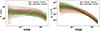 |
Fig. A.1. ICM temperature (left) and density (right) profiles of 100 randomly selected simulated galaxy clusters in THE THREE HUNDRED PROJECT. The grey lines show individual profiles, and the green and orange lines show the 30 most relaxed and disturbed clusters, respectively, according to criteria given by χ (see text for details). The solid black line shows the median of the full simulated sample. |
Appendix B: Summary of GNN model architecture and training hyper-parameters
Here we provide additional details on the GNN architecture and the hyper-parameters used for training. Table B.2 outlines the full architecture of the GNN model, including the type of each layer, the dimensionality of its input and output, and a brief description of its role in the pipeline. Table B.1 lists the optimised hyper-parameters used during training, including the learning rate, regularisation settings, and training schedule.
Optimised hyper-parameters for our fiducial five-feature GNN model.
Summary of the GNN architecture for our fiducial five-feature model used in this work, with matrix dimensions for each layer.
Appendix C: Core-excised GNN modelling
Core-excised regions in galaxy clusters are defined by excluding the innermost areas, typically within 0.15 R500, to minimise the impact of non-gravitational processes such as radiative cooling, AGN feedback, and mergers. Pratt et al. (2022) showed that these central processes introduce significant variability in the gas density, leading to a large intrinsic scatter of approximately 40%. Moreover, beyond the core, they found that thermal profiles evolve more self-similarly under the influence of gravity, resulting in a reduced scatter of around 20% at intermediate radii [0.5–0.7] R500. For example, the core-excised X-ray luminosity (LXc), measured within the [0.15–1] R500 annulus, exhibits a tight correlation with cluster mass, with a low logarithmic scatter of ∼13%. Similarly, Iqbal et al. (2023b) demonstrated that the AGN luminosity required to significantly influence the ICM out to ∼[0.1 − 0.2] R500 is comparable to the observed radio jet power, reinforcing the view that AGN feedback is the dominant heating mechanism in cluster cores.
To investigate the effect of core exclusion on mass estimation using machine learning, we also trained a GNN model without the core regions. In the core-excised setting, input features were chosen randomly such that the first data point is within the radial range [0.1-0.2] R500 and the last data point is within [0.75-2] R500, effectively excluding the central ICM region. Our results suggest that removing the core profiles only leads to a slight reduction in scatter for the high-resolution profiles (i.e. 48 bins input radial profiles). We find for the unaugmented testing sample (350 clusters), the median bias and fractional residuals to be 1.00 ± 0.06 and 0.00 ± 0.05 respectively and a scatter of 0.022 dex. However, for the observationally motivated 15 bin and 7 bin cases, for this sample, we find improved scatters of 0.023 dex and 0.024 dex, respectively, compared to the fiducial model, where the scatter for the 7 bin case was 0.036 dex. Finally, we find for this case, feature importance values to be [R, ρ, T, P, Mg]=[0.28, 0.19, 0.06, 0.1, 0.37].
Appendix D: Variants of GNN model having different feature sets
Here, we present two variants of the GNN models, differing in the number of input features. The lower-dimensional model incorporates only the density and temperature of the ICM, along with the associated radius, providing a simpler representation of the system. In contrast, the higher-dimensional model includes entropy as an additional feature, alongside the five other features considered in the fiducial model.8
Figure D.1 shows the performances of both models using the testing sample. We find that for the lower-dimensional model, the fractional residuals and mass bias to be 0.00 ± 0.06 and 1.00 ± 0.07, respectively, for the testing sample. However, here the scatter is approximately 1.5 times that of our fiducial model. Moreover, for the training sample, we have dispersion comparatively much smaller at 3% and a scatter of 0.018 dex, indicating overfitting. From the feature importance analysis, we find the relative importance as [R, ρ, T]=[0.54, 0.28, 0.17].
In contrast, the higher-dimensional model yields no improved constraints compared to the fiducial case, with a fractional residual of 0.00 ± 0.06 and a mass bias of 1.00 ± 0.05 for the testing sample. The feature importance distribution for this model is [R, ρ, T, P, K, Mg] = [0.25, 0.13, 0.03, 0.11, 0.07, 0.39], highlighting that gas mass is still the significant predictor and temperature is the least influential. Even though entropy radially increases, which parallels that of the gas mass, its ability to capture the underlying mass is still poor. Moreover, it should also be noted that the addition of entropy as a feature does not necessarily improve the model’s physical reliability as it is susceptible to observational systematics. In particular, it is known to be strongly affected by gas clumping and small-scale inhomogeneities, which can result in entropy flattening.
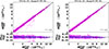 |
Fig. D.1. Performance comparison of the lower-dimensional three-feature model (left) and the higher-dimensional six-feature model (right) using the testing sample. The two subpanels show the fractional residual distributions; the solid blue line and the shaded regions represent the median and 1σ dispersion, respectively. The lower-dimensional model yields a relatively large scatter of 0.038 dex for the testing sample. In contrast, the higher-dimensional model shows no improved constraints compared to the fiducial model, with a scatter of 0.026 dex for the testing sample. |
Appendix E: Redshift dependence on model training
In this Appendix, we investigate the impact of incorporating redshift information during the model training process. Specifically, the model was trained using two distinct redshift snapshots: z = 0.33 and z = 0.06, and evaluated on an independent snapshot at z = 0.95. This set-up enabled an assessment of the model’s ability to generalise across different epochs of cosmic time.
A data augmentation strategy, similar to that employed in the development of the fiducial model, was also applied. In this case, however, both the unaugmented training and testing samples were randomly assigned redshifts within the range 0 ≤ z ≤ 1.2. By systematically using different redshift bins for the unaugmented samples during training and testing, we explored the model’s sensitivity to cosmic evolution and examined its implications for astrophysical interpretation.
Figure E.1 presents the distribution of GNN predicted cluster masses versus the true cluster masses for both the training and testing samples. We note that since the testing sample is at high redshift, it contains fewer massive clusters compared to the training sample. As expected, the model’s predictions for the training sample remain effectively unbiased, with predicted values closely following the true cluster masses with a scatter of 0.025 dex. For the testing sample, we observe a bias of (1 − b) = 0.96 ± 0.08 and a scatter of 0.061 dex. While this bias is statistically consistent with unity, it suggests a slight underestimation of cluster masses on average. This also shows that there is a significant over-fitting during the training stage. These findings highlight the importance of incorporating redshift-specific information during training to improve model generalisation and ensure accurate mass predictions across a wide span of cosmic time.
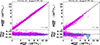 |
Fig. E.1. GNN predicted masses, |


Appendix F: Comparison of the M with M
 and M
and M masses for REXCESS sample
The X-ray derived mass, M , is derived from observations linked to the thermal bremsstrahlung emission of the ICM. Here, the observable YX= Mg× T is linked to M
 . For our work, we consider M500 values derived from Pratt et al. (2022). The cluster masses were estimated using the YX mass proxy. This proxy is based on the assumption of hydrostatic equilibrium and has been shown to correlate tightly with the total cluster mass. Using XMM-Newton observations of 93 SZE-selected galaxy clusters, they also derived a scaling relation between the core-excised X-ray luminosity (LXc) and the total mass proxy M
 , finding a logarithmic intrinsic scatter of approximately 0.13 dex. Table F.1 summarises the results of our analysis using the REXCESS sample.
Results with REXCESS sample. Columns: (1) Cluster name, (2) Redshift, (3) Mass obtained using from YX-M ,(4) GNN estimated mass, M
 (this work).
For the REXCESS sample, we find the following best-fitting relations for the M and M
and M biases with respect to the GNN masses
 (F.1)
(F.1)
We also quantify the mass bias (1 − b) as a function of M , yielding
 (F.2)
(F.2)
We find a mass dependence of bias at around 3σ for M -M
-M relation.
Appendix G: Comparison of the M with hydrostatic and M
 masses for X-COP sample
Eckert et al. (2019) not only estimated the hydrostatic masses (M ) but also proposed a method to estimate the total mass which includes the contribution from non-thermal pressure (Nelson et al. 2014) (M
 ). They considered a functional form for the non-thermal pressure derived from hydrodynamical simulations along with the hydrostatic approximation while assuming a universal gas mass fraction at the varial radius. Table G.1 summarises the comparison of cluster mass estimates for the X-COP sample derived using various methodologies.
Results with X-COP sample. Columns: (1) Cluster name, (2) Redshift, (3) Mass obtained using from YSZ-M , (4) Hydrostatic mass, M
 , (5) Hydrostatic mass corrected with non-thermal pressure, M
 , (6) GNN estimated mass, M
 (this work).
For the X-COP sample, we find the following best-fitting relations for the M , M
, M and M
and M biases with respect to the GNN masses
 (G.1)
(G.1)
The mass bias (1 − b) as a function of M for the X-COP sample gives
 (G.2)
(G.2)
For the X-COP sample, we find weak evidence, at the 2σ level, for a mass dependent bias in the SZ masses relative to the GNN masses.
All Tables
Summary of the GNN architecture for our fiducial five-feature model used in this work, with matrix dimensions for each layer.
Results with REXCESS sample. Columns: (1) Cluster name, (2) Redshift, (3) Mass obtained using from YX-M,(4) GNN estimated mass, M (this work).
Results with X-COP sample. Columns: (1) Cluster name, (2) Redshift, (3) Mass obtained using from YSZ-M, (4) Hydrostatic mass, M, (5) Hydrostatic mass corrected with non-thermal pressure, M, (6) GNN estimated mass, M (this work).
All Figures
|
Fig. 1. Comparison of the hydrostatic mass estimates |
| In the text | |
|
Fig. 2. Pressure profiles of clusters with low and high fractional dispersions in M500 derived using hydrostatic equilibrium. The grey lines show the pressure profiles of the 50 clusters having the lowest (left panel) and highest (right panel) fractional dispersions. The thick red lines indicate the corresponding median profiles. The bottom panel displays the ratio of reconstructed to true pressure profiles. In the right panel, we have also plotted the median profile for the lowest dispersion set with a thick blue line for comparison. The insets illustrates the distribution of the relaxation parameter χ for the same clusters. |
| In the text | |
|
Fig. 3. Number distribution of galaxy clusters in the THE THREE HUNDRED PROJECT as a function of |
| In the text | |
|
Fig. 4. Train and test loss in the evaluation mode over epochs for one of the ensemble models. Both train and test losses indicate consistent learning, with the final loss at around 0.02 for the training and testing sets. |
| In the text | |
|
Fig. 5. Distribution of GNN predicted masses, |
| In the text | |
|
Fig. 6. Histogram of residual distributions for the entire unaugmented test sample of 350 galaxy clusters, and for the 50 most relaxed and 50 most disturbed clusters within this sample. The vertical dashed lines show the corresponding median of distributions. We find comparable performance of the GNN model across different dynamical states. |
| In the text | |
|
Fig. 7. Comparison of predicted and true galaxy cluster masses for an unaugmented test sample of 350 clusters. The black line represents a 1-to-1 relation. The magenta, orange, and green points represent predictions using ICM profiles truncated respectively at 2R500, R500, and 0.75 R500, with 48, 15, and 7 bins. The inset shows the corresponding fractional residuals; the vertical lines represent the medians. |
| In the text | |
|
Fig. 8. 1σ GNN model uncertainty, σGNN, estimated using KDE-based SBI, as a function of the true cluster mass |
| In the text | |
|
Fig. 9. Extrapolation performance of the GNN model when evaluated with input data restricted to the inner regions. The plot shows predicted vs. true cluster masses for three cases where the available ICM data extends only up to 0.5 R500, 0.4 R500, and 0.3 R500, corresponding to Case A, B, and C in the text and 7, 5, and 5 radial bins, respectively. |
| In the text | |
|
Fig. 10. Comparison of GNN and hydrostatic equation predictions for M500 using an unaugmented test sample of 350 galaxy clusters. The black line represents a 1-to-1 relation. The magenta and orange points respectively compare the GNN predictions and the hydrostatic predictions with the true masses. The inset shows the distribution of residuals for both approaches; the vertical lines show the median of the distributions. |
| In the text | |
|
Fig. 11. Average feature importance for predicting M500 as a function of input features. Shown are the relative importance of the five features, i.e. density (ρ), temperature (T), pressure (P), gas mass (Mg), and radius (R). |
| In the text | |
|
Fig. 12. Left panel: Comparison of masses derived from the GNN model with those obtained from the SZ scaling relation. The black line represents the ideal 1-to-1 relation. The inset shows the distribution of fractional residuals. The right panel shows the bias in the SZ determined mass (M |
| In the text | |
|
Fig. A.1. ICM temperature (left) and density (right) profiles of 100 randomly selected simulated galaxy clusters in THE THREE HUNDRED PROJECT. The grey lines show individual profiles, and the green and orange lines show the 30 most relaxed and disturbed clusters, respectively, according to criteria given by χ (see text for details). The solid black line shows the median of the full simulated sample. |
| In the text | |
|
Fig. D.1. Performance comparison of the lower-dimensional three-feature model (left) and the higher-dimensional six-feature model (right) using the testing sample. The two subpanels show the fractional residual distributions; the solid blue line and the shaded regions represent the median and 1σ dispersion, respectively. The lower-dimensional model yields a relatively large scatter of 0.038 dex for the testing sample. In contrast, the higher-dimensional model shows no improved constraints compared to the fiducial model, with a scatter of 0.026 dex for the testing sample. |
| In the text | |
|
Fig. E.1. GNN predicted masses, |
| In the text | |
Current usage metrics show cumulative count of Article Views (full-text article views including HTML views, PDF and ePub downloads, according to the available data) and Abstracts Views on Vision4Press platform.
Data correspond to usage on the plateform after 2015. The current usage metrics is available 48-96 hours after online publication and is updated daily on week days.
Initial download of the metrics may take a while.