| Issue |
A&A
Volume 704, December 2025
|
|
|---|---|---|
| Article Number | A152 | |
| Number of page(s) | 18 | |
| Section | Extragalactic astronomy | |
| DOI | https://doi.org/10.1051/0004-6361/202555928 | |
| Published online | 05 December 2025 | |
Semiempirical constraints on the HI mass function of star-forming galaxies and ΩHI at z∼ 0.37 from interferometric surveys
1
Département d’Astronomie, Université de Genève, Chemin Pegasi 51, CH-1290 Versoix, Switzerland
2
Department of Astrophysics, University of Zurich, Winterthurerstrasse 190, CH-8057 Zürich, Switzerland
3
Department of Physics and Astronomy, Università degli Studi di Padova, Vicolo dell’Osservatorio 3, I-35122 Padova, Italy
4
INAF – Osservatorio Astronomico di Padova, Vicolo dell’Osservatorio 5, I-35122 Padova, Italy
5
Department of Physics and Astronomy, University of the Western Cape, Robert Sobukwe Rd, 7535 Bellville, Cape Town, South Africa
6
Inter-university Institute for Data Intensive Astronomy, Department of Astronomy, University of Cape Town, 7701 Rondebosch, Cape Town, South Africa
7
Inter-university Institute for Data Intensive Astronomy, Department of Physics and Astronomy, University of the Western Cape, 7535 Bellville, Cape Town, South Africa
8
INAF – Istituto di Radioastronomia, Via Gobetti 101, 40129 Bologna, Italy
9
Astrophysics, University of Oxford, Denys Wilkinson Building, Keble Road, Oxford OX1 3RH, UK
10
Department of Physics and Astronomy, University of the Western Cape, Cape Town 7535, South Africa
⋆ Corresponding author: This email address is being protected from spambots. You need JavaScript enabled to view it.
Received:
12
June
2025
Accepted:
15
September
2025
Abstract
Context. The H I mass function (HIMF) is a crucial tool for understanding the evolution of the H I content in galaxies over cosmic time and, hence, to constraining both the baryon cycle in galaxy evolution and the reionization history of the Universe.
Aims. We aim to derive semiempirical constraints at z ∼ 0.37 by combining literature results on the stellar mass function from optical surveys with recent findings on the MHI − M⋆ scaling relation derived via spectral stacking analysis applied to 21 cm line interferometric data from the MIGHTEE and CHILES surveys, conducted with the MeerKAT and VLA radio telescopes, respectively.
Methods. We drew synthetic stellar mass samples directly from the publicly available results underlying the analysis of the COSMOS2020 galaxy photometric sample. We then converted M⋆ into MHI using analytical fitting functions to the data points from H I stacking. We next fit a Schechter function to the median HIMF from all the samples via Monte Carlo Markov chains. We finally derived the posterior distribution for ΩHI by integrating the models for the HIMF built from the posteriors samples of the Schechter parameters.
Results. We find a deviation of the HIMF at z ∼ 0.37 from the results at z ∼ 0 from the ALFALFA survey and at z ∼ 1 from uGMRT data. Our results for ΩHI are in broad agreement with other literature results and follow the overall trend on ΩHI as a function of redshift. The derived value ΩHI = (7.02+0.59−0.52) × 10−4 at z ∼ 0.37 from the combined analysis deviates by ∼2.9σ from the ALFALFA result at z ∼ 0.
Conclusions. Our findings regarding the HIMF and ΩHI derived from deep, state-of-the-art interferometric surveys differ from previous literature results at z ∼ 0 and z ∼ 1. We are unable to confirm at this stage whether these differences are due to cosmic evolution consistent with a smooth transition of the H I content of galaxies over the last 8 Gyr or due to selection biases and systematics.
Key words: galaxies: evolution / galaxies: ISM
© The Authors 2025
 Open Access article, published by EDP Sciences, under the terms of the Creative Commons Attribution License (https://creativecommons.org/licenses/by/4.0), which permits unrestricted use, distribution, and reproduction in any medium, provided the original work is properly cited.
This article is published in open access under the Subscribe to Open model. This email address is being protected from spambots. You need JavaScript enabled to view it. to support open access publication.
1. Introduction
Neutral atomic hydrogen (hereafter H I) plays a key role in astrophysics and cosmology. The distribution of H I in the Universe is driven by the complex interplay of astrophysical and cosmological effects. The abundance of H I in the large-scale structure is regulated by the nonlinear formation and evolution of the cosmic web (e.g., Martizzi et al. 2019; Galárraga-Espinosa et al. 2021; Sinigaglia et al. 2021, 2024). Once galaxies form within dark matter haloes due to the conversion of the intra-halo H I to molecular hydrogen and gravitational collapse (e.g., Somerville & Davé 2015; Vogelsberger et al. 2020; Primack 2024), the H I constitutes the main raw fuel for star formation and is one of the major ingredients contributing to the baryon cycle and in regulating the galaxy mass assembly (e.g., Blitz & Rosolowsky 2006; Bigiel et al. 2008; Sternberg et al. 2014). For these reasons, constraining the H I cosmic density parameter (ΩHI) and the H I mass function (HIMF) over cosmic time is of paramount importance to answering profound questions about the Universe regarding cosmic reionization (e.g., Koopmans et al. 2015; DeBoer et al. 2017), galaxy mass assembly, and the time evolution of the star formation rate density (e.g., Huang et al. 2012; Maddox et al. 2015; Catinella et al. 2018; Sinigaglia et al. 2022; Bianchetti et al. 2025). H I can even be used to infer cosmological information such as the nature of dark matter (e.g., Pinetti et al. 2020; Bauer et al. 2021; Bañares-Hernández et al. 2023) and dark energy (e.g., Santos et al. 2015; Zhang et al. 2023; Berti et al. 2024), as well as to test the Λ cold dark matter model and other alternative theories of gravity with resolved galaxy rotation curves (e.g., O’Brien et al. 2018).
Measuring ΩHI and the HIMF is, however, a challenging task. Due to the intrinsic faintness of the 21 cm line and the limited sensitivity of the majority of the existing radio telescopes, a direct measurement of the H I emission has so far been possible only out to relatively low redshifts. Current existing constraints on ΩHI and the HIMF based on a statistically large sample of H I galaxies are limited to the nearby Universe (z ≲ 0.1; e.g., Zwaan et al. 2003; Martin et al. 2010; Jones et al. 2018; Ponomareva et al. 2023). The most accurate measurement of the HIMF is that presented by the full ALFALFA survey at z ≤ 0.06, which comprises approximately 31, 500 H I sources (Jones et al. 2018). At z > 0.1, only a few studies have reported measurements of the HIMF and ΩHI based on direct H I detection, such as those based on data from the AUDS survey at z = 0.16 (Hoppmann et al. 2015) and the BUDHIES survey at z = 0.2 (Gogate 2022). Nonetheless, the available number of sources is still limited to a few tens to hundreds, implying a considerable uncertainty, especially on the high-mass end of the HIMF. In addition, BUDHIES targeted dense fields, which may not be representative of the global galaxy population. Alternative approaches to estimating ΩHI involve measuring the average H I mass in galaxies (e.g., Lah et al. 2007; Delhaize et al. 2013; Rhee et al. 2016, 2018; Hu et al. 2019), using the cross-correlation between optical galaxies and H I intensity mapping (Chang et al. 2010; Masui et al. 2013; Wolz et al. 2022; Cunnington et al. 2023), or relying on the H I absorption features observed in damped Lyα systems (e.g., Rao et al. 2006; Noterdaeme et al. 2012; Crighton et al. 2015; Rao et al. 2017). These methods, however, do not yield a measurement of the HIMF, only an estimate of the total H I cosmic density.
A novel semiempirical method – only possible thanks to the improved sensitivity of state-of-the art radio telescopes such as the MeerKAT and the upgraded Giant Metrewave Radio Telescope (uGMRT) – has recently emerged as an indirect but cheap alternative to direct H I detection to constrain ΩHI and the HIMF at intermediate and high redshifts. This method consists of exploiting robust measurements from the literature of the galaxy stellar mass or luminosity function across redshifts and to converting it to H I via a scaling relation, measured with a H I stacking approach. Bera et al. (2022) and Chowdhury et al. (2024) pioneered this technique and used it to measure the HIMF at z ∼ 0.35 and z ∼ 1, respectively. They exploited the B-band magnitude (MB) luminosity function and used the MHI − MB scaling relation for star-forming galaxies; this relation was measured using a 21 cm line spectral stacking approach applied to uGMRT observations and converted from MB to MHI to obtain the HIMF.
The H I intensity mapping technique will also eventually be capable of providing (indirect) constraints on ΩHI and the HIMF. Paul et al. (2023) reported the first measurement of the HIMF from a H I intensity mapping experiment, a measurement of the H I intensity mapping power spectrum at z ∼ 0.32. They also used a halo model approach to constrain the HIMF, following Chen et al. (2021).
In this work we followed a methodology similar in spirit to that used by Bera et al. (2022) and Chowdhury et al. (2024). We combined the most recent measurements of the stellar mass function of star-forming galaxies in the COSMOS field at 0.2 < z < 0.5 by Weaver et al. (2023) and of the MHI − M⋆ scaling relation of star-forming galaxies at 0.22 < z < 0.49 (median redshift z ∼ 0.37) by Bianchetti et al. (2025) from the H I stacking analysis of two state-of-the-art deep H I interferometric surveys, MIGHTEE (Jarvis et al. 2016) and CHILES (Fernández et al. 2013); both cover the COSMOS field (Scoville et al. 2007). With these tools, we derived novel indirect semiempirical constraints on the HIMF of star-forming galaxies and the cosmic H I density parameters (ΩHI) at z ∼ 0.37.
The paper is organized as follows. Section 2 introduces the optical and H I data used in this work. Section 3 summarizes the main features of the cosmological hydrodynamic simulations we used to compare our results with. We present our methodology in Sect. 4. Section 5 presents the analysis, the results of our predictions, and a discussion. We conclude in Sect. 6.
Throughout this work we adopt the following cosmological parameters: Ωm = 0.3, ΩΛ = 0.7, and H0 = 70.0 km s−1 Mpc−1. When relevant, we have rescaled the results from other literature results to the match the cosmological parameters adopted herein.
2. Data from optical and H I surveys in the COSMOS field
In this section we summarize the main features of the data from optical surveys included in the COSMOS2020 catalog (Weaver et al. 2022), from the MIGHTEE and the CHILES 21 cm line interferometric surveys, as well as the main stacking results from Bianchetti et al. (2025). We refer to Bianchetti et al. (2025), for a more detailed description of all the items described in what follows.
2.1. The COSMOS2020 sample and the stellar mass function
The optical catalog underlying the stacking analysis performed by Bianchetti et al. (2025) was built through a cross-match between the COSMOS2020-CLASSIC1 photometric catalog (Weaver et al. 2022) and a spectroscopic catalog assembled by merging three different catalogs covering the COSMOS field: the COSMOS spec-z compilation (Khostovan et al. 2025), the DEVILS survey catalog (Davies et al. 2018) and the DESI survey Early Data Release catalog (DESI Collaboration 2024). First, Bianchetti et al. (2025) selected only spectroscopic sources in the COSMOS field (Scoville et al. 2007) and at 0.22 < z < 0.49 (median redshift z ∼ 0.37), i.e., within a subset of the volume probed by the MIGHTEE and CHILES datasets (see Sect. 2.2). They performed a positional cross-match (with matching radius = 1 arcsec) between the spectroscopic and the photometric catalog. The photometric catalog includes galaxy properties obtained through spectral energy density fitting performed with the LePhare code (Ilbert et al. 2006; Arnouts & Ilbert 2011). Therefore, after the cross-match, they retrieved from the photometric catalog all the aforementioned photometrically derived parameters for each of the sources in the spectroscopic catalog. Star-forming galaxies were then selected using the in-built color-color selection in the (NUV − r)/(r − J) rest-frame plane. Further quality cuts were then applied to ensure the highest possible reliability, including redshift quality cuts and photometric redshift outliers exclusion.
Weaver et al. (2022, 2023) have shown that the COSMOS photometric sample is complete in stellar mass down to log10(M⋆/M⊙)≈8 at z < 0.5.
In this work we also made use of the results on the stellar mass function in the COSMOS field as measured from the COSMOS2020 catalog (Weaver et al. 2023). Weaver et al. (2023) performed a detailed study of the stellar mass sample from COSMOS2020, deriving the stellar mass functions for the total, star-forming, quiescent populations at 0.2 < z < 0.5, as well as in several higher redshift ranges. The splitting of the galaxy population into star-forming and quiescent was performed according to the same color criterion mentioned above. These aspects, together with the fact that the underlying photometric catalog is the same, make the stellar mass function derived by Weaver et al. (2023) as the ideal candidate to be used in this work. Weaver et al. (2023) used a Markov chain Monte Carlo method to fit a double Schechter profile to the resulting stellar mass function:
![Mathematical equation: $$ \begin{aligned} \Phi ~ \mathrm{d}\log _{10}&(M_\star /\mathrm{M}_{\odot }) = \log (10)\exp \left(-10^{\log _{10}(M_\star /\mathrm{M}_{\odot })-\log _{10}(\tilde{M}/\mathrm{M}_{\odot })}\right) \nonumber \\&\times \biggl [ \tilde{\Phi }_1 \left(10^{\log _{10}(M_\star /\mathrm{M}_{\odot })-\log _{10}(\tilde{M}/\mathrm{M}_{\odot })}\right)^{\alpha _1 +1}\nonumber \\&+ \tilde{\Phi }_2 \left(10^{\log _{10}(M_\star /\mathrm{M}_{\odot })-\log _{10}(\tilde{M/\mathrm{M}_{\odot }})}\right)^{\alpha _2 +1} \biggr ] ~\mathrm{d}\log _{10}(M_\star /\mathrm{M}_{\odot }). \end{aligned} $$](/articles/aa/full_html/2025/12/aa55928-25/aa55928-25-eq2.gif) (1)
(1)
For the star-forming mass-complete galaxy subsample at 0.2 < z < 0.5, Weaver et al. (2023) found the following best-fitting parameters:
The best-fitting values quoted above consist of the median of the posteriors of the parameters. While the median stellar mass function can then be readily obtained by substituting those values for the parameters inside Eq. (1), we would not be properly accounting for the parameters uncertainty and covariance. In Sect. 4 we outline the Monte Carlo procedure used throughout this work, in which we needed to obtain many samples for the stellar mass function varying the best-fitting parameters within their uncertainty, and hence, correctly accounting for their covariance. To do so, instead of resorting to the best-fitting median values of posteriors, we randomly drew samples directly from the Markov chain posteriors from Weaver et al. (2023), made publicly available2. This allowed us to correctly account for uncertainties on the stellar mass function in a Bayesian fashion within our framework.
2.2. The MIGHTEE and CHILES surveys
MIGHTEE (Jarvis et al. 2016) is a survey conducted with MeerKAT radio telescope. The MeerKAT radio interferometer (Jonas & MeerKAT Team 2016) consists of 64 offset Gregorian dishes equipped with receivers in the UHF band (580 MHz < ν < 1015 MHz), L band (900 MHz < ν < 1670 MHz), and S band (1750 MHz < ν < 3500 MHz), and serves as a precursor to the Square Kilometre Array (SKA). MIGHTEE is an L-band continuum, polarization, and spectral-line large survey conducted with MeerKAT, utilizing spectral and full Stokes mode observations. It covers four deep extragalactic fields (COSMOS, XMM-LSS, ECDFS, and ELAIS-S1), chosen because of their extensive multiwavelength coverage from previous and ongoing observations. For this study we used results derived for the MIGHTEE-H I Early Science spectral line data from MIGHTEE (Maddox et al. 2021) covering the COSMOS field with a single pointing within the redshift range of 0.22 < z < 0.49, with an effective exposure time of approximately 23 hours. The MIGHTEE beam is approximately 17.2″ × 13.9″ at z ∼ 0.37 (∼90 × 73 kpc2). The median H I noise RMS of the cubes increases as the frequency decreases, ranging from 85 μJy beam−1 at ν ∼ 1050 MHz to 135 μJy beam−1 at ν ∼ 950 MHz at a spectral resolution (channel width) of 209 kHz.
CHILES is a deep-field H I survey, carried out with the VLA and imaging H I over a contiguous redshift range of 0 < z < 0.49 for the first time (Fernández et al. 2013). The pointing was centered on RA(J2000) 10h01m24s and Dec(J2000) 2d21m00s. It samples a subregion of the COSMOS field; therefore, it provides an independent measurement of the same patch of sky as the MIGHTEE survey. The 25-meter diameter antennas of the VLA provide a field of view of around 0.5 deg at 1.4 GHz. Due to the rotating VLA configurations, the CHILES observations were split into five observing epochs spaced approximately 15 months apart. In this study we used results from successfully processed data from all five of the observing epochs, amounting to approximately 800 observation hours (approximately 600 on-source hours). The VLA-B configuration was used, achieving a beam size of approximately 7.2″ × 6.4″ at z ∼ 0.37 (≈38 × 33 kpc2). The datacube comprises 125 kHz wide spectral channels at z ∼ 0.37, covering a wide range of frequencies (950 − 1420 MHz). The RMS ranges between 30 and 50 μJy beam−1 in this range.
2.3. Stacking results from MIGHTEE and CHILES
A fundamental ingredient upon which this work is based consists of the stacking results from Bianchetti et al. (2025). They performed a 21 cm line stacking analysis in different stellar mass bins for the star-forming galaxy population, with the aim of measuring the MHI − M⋆ scaling relation from the combination of the MIGHTEE and CHILES surveys. While a detailed summary of the results goes beyond the scope of this paper (we refer directly to Bianchetti et al. (2025) for it), we report in Table 1 the numerical values for the data points. In particular, we notice that for the combined stacking the larger statistics allowed the authors to split the sample into four stellar mass bins, while for the MIGHTEE and CHILES separate stacking analyses, it was possible to split the galaxy population only into three stellar mass bins to be able to detect the H I signal in all of them. This aspect will become important later on in the paper when describing the fitting strategy for the MHI − M⋆ relation.
Data points from the H I spectral stacking analysis used in this work.
3. Reference cosmological hydrodynamic simulations
In this section we summarize the main features of the two cosmological hydrodynamic simulation that we used in this study for comparison with our results, SIMBA (Davé et al. 2019) and IllustrisTNG (Nelson et al. 2019). In what follows we describe only the pieces of information relevant for this work, and refer to Davé et al. (2019) and Nelson et al. (2019) for a thorough description of the simulations.
3.1. SIMBA
SIMBA is a cosmological hydrodynamic simulation run with the GIZMO mesh-less finite mass hydrodynamics. It was run in three different combinations of box sizes and resolutions: with 2 × Ndm = 10243 particles (namely, Ndm = 10243 dark matter particles and Ngas = 10243 gas elements) in a V = (100 Mpc h−1)3 comoving volume (hereafter SIMBA-100), 2 × Ndm = 5123 in a volume V = (50 Mpc h−1)3 (hereafter SIMBA-50), and 2 × Ndm = 5123 in a volume V = (25 Mpc h−1)3, i.e., at higher resolution with respect to SIMBA-100 and SIMBA-50. The SIMBA fiducial model adopts and updates star formation and feedback sub-grid prescriptions used in the MUFASA simulation (Davé et al. 2016), and introduces the treatment of black hole growth and accretion from cold and hot gas. Moreover, models for on-the-fly dust production, growth, and destruction, and H I and H2 abundance computation are implemented (see Davé et al. 2019, and references therein for details). SIMBA has been shown to reproduce several observables, among which the galaxy stellar mass functions at z < 6 and the M* − SFR main sequence. In addition to the full feedback model, multiple runs of SIMBA-50 were performed, adopting variations around the full feedback model. The different feedback variations are described in Sect. 5.4. The H I masses in SIMBA were computed by assigning all the gas in the halo to its most bound galaxy within the halo (Davé et al. 2020) and by assuming the sub-grid model by Krumholz & Gnedin (2011). In this model, the H2 fraction is computed based on the local metallicity and gas column density, modified to account for variations in resolution (Davé et al. 2016). The H I fraction is then computed by subtracting off the H2 fraction from the total cold gas.
In this work we made use of the publicly available galaxy catalogs at z ∼ 0.365 for SIMBA-100 and for all the SIMBA-50 boxes. Consistently with the observational sample selection by Bianchetti et al. (2025), we selected only star-forming galaxies with log10(M*/M⊙) > 8 by separating the star-forming and quenched populations in the M* − SFR plane. After a detailed inspection of the M* − SFR plane, we heuristically flagged as star-forming those galaxies with log10(SFR/(M⊙ yr−1)) > 0.9 × log10(M*/M⊙)−9.2 at z ∼ 0.365 (see, Sinigaglia et al. 2022).
3.2. IllustrisTNG
IllustrisTNG is a suite of cosmological, gravo-magnetohydrodynamic simulations run with the moving-mesh code AREPO (Springel 2010). IllustrisTNG consists of an improved and updated version of the original Illustris simulations suite (Nelson et al. 2015), and includes the following baryon physics mechanisms, among others: primordial and metal-line radiative cooling with an ionizing background radiation field, stochastic star formation, an effective equation of state model accounting for the two phases of the interstellar medium, evolution of stellar populations, stellar feedback, seeding and growth of supermassive black holes, AGN feedback (and in particular, energy release from high- and low-accretion rates), and the treatment of magnetic fields.
In this work we used the following larger-volumes runs: IllustrisTNG-100, run with N = 2 × 18203 resolution elements and in volume V = (75 h−1 Mpc)3, and IllustrisTNG-300, run with N = 2 × 25003 resolution elements and in volume V = (205 h−1 Mpc)3.
As estimates for the H I masses, we used the catalogs released by Diemer et al. (2018). Therein, the authors performed a detailed splitting of the cold gas into its atomic and molecular phases, by adopting different sub-grid models. Out of the models tested in Diemer et al. (2018), we chose to use the values for MHI obtained through the model by Gnedin & Kravtsov (2011), which was calibrated on high-resolution simulations designed to explicitly solve for radiative transfer on the fly during the simulation. Specifically, we used the catalogs at z = 0.5, i.e., the closest redshift to that of our data available. Even though it does not match perfectly the redshift we are working at, it should provide a good qualitative proxy for the HIMF at intermediate redshift such as the one from this work.
We selected star-forming galaxies from IllustrisTNG using the same criterion used for SIMBA, for consistency. This is a safe choice since the two simulations have been separately shown to reproduce the star formation rate–M⋆ plane well.
4. Methods
In this work we largely followed the methodology pioneered by Bera et al. (2022). We aimed to derive semiempirical constraints on the HIMF and the H I cosmic density parameter ΩHI passing from stellar mass to a H I mass by means of a MHI − M⋆ scaling relation. In this way, we leveraged the well-studied evolution with redshift of the stellar mass function and only assumed a scaling relation measured via spectral stacking.
We adopted the following forward-modeling:
-
We considered a complete stellar mass sample from the COSMOS2020 stellar mass function at 0.2 < z < 0.5 tabulated in Weaver et al. (2022);
-
We assumed the MHI − M⋆ scaling relation measured via H I spectral stacking from the combination of MIGHTEE and CHILES datasets and presented in Bianchetti et al. (2025). As discussed in more detail later on in the paper, this step requires an adequate assumption on the scatter of the MHI − M⋆ relation. While the stacking procedure yields the average MHI in each of the studied stellar mass bins, it does not provide any information about the scatter;
-
Once we converted the stellar mass sample into a H I mass sample, it was straightforward to build the HIMF.
-
We fit a Schechter function to the HIMF, for all values of MHI above the estimated MHI completeness limit.
-
We integrated the HIMF and computed the total H I density ρHI and then computed ΩHI = ρHI/ρc, where ρc is the critical density of the Universe.
In what follows, we describe in detail each of the points outlined above.
4.1. The reference stellar mass function
As mentioned in Sect. 2.1, we adopted the stellar mass function for star-forming galaxies at 0.2 < z < 0.5 from the COSMOS2020 photometric catalog (Weaver et al. 2023). We took advantage of the publicly available posterior distributions of the parameters for the fitted double Schechter profile as follows.
For each stellar mass function obtained by substituting the parameters from the posteriors into the model, we drew a “synthetic” galaxy sample at log10(M⋆/M⊙) > 8, i.e., the same lower M⋆ limit used by Bianchetti et al. (2025). To adequately account for the uncertainty coming from the limited sample size, we fixed it to those from the samples studied in Bianchetti et al. (2025). Henceforth, we sampled from the stellar mass function N = 6, 598 galaxies for the analysis based on the full stacking results from the combination of MIGHTEE and CHILES. We adopted N = 4, 576 galaxies for the analysis based on MIGHTEE results, and N = 2022 for the analysis based on CHILES results when studying the consistency of the HIMF derived separately from the two surveys in Appendix A. We explore the impact of the assumed sample size in Appendix E.
4.2. Converting stellar masses into HI masses
To pass from the stellar mass sample obtained as described in Sect. 4.1, we adopted the scaling relation from Bianchetti et al. (2025). As described in Sect. 2.3, therein the authors performed H I stacking in 4 stellar mass bins for the combined case, and 3 stellar mass bins separately for MIGHTEE and CHILES. For the different cases, the authors fitted a single power law model of the type log10(MHI/M⊙) = blog10(M⋆/M⊙)+c, with b and c free parameters, i.e., a linear function in logarithmic space (hereafter the linear model). In this work, we generalized this framework by also fitting a second-order polynomial in logarithmic space, parametrized as log10(MHI/M⊙) = alog10(M⋆/M⊙)2 + blog10(M⋆/M⊙)+c (hereafter the polynomial model). This higher-order polynomial allows us to capture a potential deviation from a single power law model – i.e., a linear model in logarithmic space – which has been shown to be the case for results at z ∼ 0 based on direct H I detection (see, e.g., Huang et al. 2012; Maddox et al. 2015; Parkash et al. 2018). Such a phenomenon is typically described by means of a functional form that decreases more quickly toward low MHI and flattens toward high MHI values. To account for this behavior, the following double power law model was proposed (e.g., Maddox et al. 2015; Parkash et al. 2018; Pan et al. 2023):
 (2)
(2)
with M0, Mtr, α and β free parameters. We notice that α and β denote the low- and high-mass end slopes and that this model reduces to the single power law model when α = β. In this work, since we have at most four data points available for the combined stacking case, we cannot fit this model – which has four free parameters – but at most a model with three free parameters; otherwise, we would be overfitting our data. This motivates further the choice of a second-order polynomial, as alternative to a linear fit. Later on in the paper we show that the best-fitting polynomial model qualitatively reproduces the same trend as the double power law model discussed above. We notice that for the cases of the stacking performed separately on MIGHTEE and CHILES, for which we have only three data points each, we are again in a situation where a full fit of a second-order polynomial with three free parameters would result in overfitting. We discuss this issue in Sect. 5.1 and show how we reduced the number of free parameters from three to two to also have a well-defined fit in the MIGHTEE and CHILES separate cases.
We estimated the best-fitting parameters for the linear and polynomial models and the related uncertainties by means of a bootstrap resampling (see Bianchetti et al. 2025). While this has already been performed by Bianchetti et al. (2025) for the linear model, it had not been done for the polynomial one. We resampled the data points underlying the fit by randomly sampling a lognormal uncertainty based on the uncertainty on the estimation of MHI of each data point3. For each bootstrap sample, we then applied the full forward model and obtained the HIMF.
In addition to the best-fitting MHI − M⋆, which provides only the average trend, we also needed to model the scatter of the relation. Because the scatter is not measurable via traditional stacking, which yields only the average MHI value in each stellar mass bin but not the underlying dispersion, we needed to make an assumption of a credible value for the scatter. Bera et al. (2022) show that properly modeling the scatter is of crucial importance to capture the behaviour of the HIMF. Therein, the authors performed stacking in MB intervals and derive the HIMF by means of the MHI − MB relation. They assumed a scatter σ = 0.26 dex – the same as in the Local Universe — which was proven to correctly reproduce the HIMF from ALFALFA at z ∼ 0.
In this work, since we used a different scaling relation, we also needed to assume a different value for the scatter. We made the same assumption as Bera et al. (2022) and used the value of the scatter at z ∼ 0 from the MHI − M⋆ scaling relation measured by the xGASS survey (Catinella et al. 2018), i.e., σ = 0.39 dex. We study the specific impact of the scatter in our framework in Appendix B, where we show that the value for the scatter largely affects the high-mass end of the HIMF. Specifically, the high-mass end of the HIMF is shown to increase with increasing value of the scatter. Therefore, we incorporated an additional source of uncertainty on the scatter as follows. For each step of our Monte Carlo procedure, we added to the scatter an error randomly sampled from a Gaussian distribution with zero mean and standard deviation σerr = 0.05. The value for this additional uncertainty contribution is motivated by covering the range of values σ = (0.39 ± 0.05) dex, i.e., a conservatively wide range of credible values that the scatter can assume according to z = 0 observations. In this way, we self-consistently accounted for the error on the scatter in each of the sampling steps and propagated the related uncertainty throughout our forward model. In Appendix B we show that this source of stochasticity yields no significant difference on the uncertainties on the best-fitting parameters of the HIMF with respect to the case where no scatter is assumed, nor introduces any obvious systematic shift in the median values. Therefore, in the remainder of the paper we assume as the fiducial configuration the one that includes the error on the scatter, even though we argue that this has been shown to have little impact. In addition, in Appendix C we study the impact of relaxing the assumption of a Gaussian symmetric scatter in log space, and test whether adopting a more realistic asymmetric functional form has any impact on the final results. Specifically, we modeled the scatter as a lognormal distribution in log space with parameters determined by fitting the true H I distribution at fixed M⋆ as measured by the cross-matched SDSS-ALFALFA catalog Durbala et al. (2020). We find that accounting for an asymmetric scatter has no significant impact with respect to assuming a symmetric scatter, and stick to the simpler Gaussian model for simplicity.
At the end of this procedure, we obtained a sample of HIMFs from which we computed the bin-wise median and standard deviation, which represent, respectively, the final HIMF and its associated uncertainty. This defines our “measured” HIMF.
4.3. Fitting the HI mass function and deriving ΩHI
After having obtained the average HIMF and the associated uncertainty, as described in Sect. 4.2, we fit a single Schechter profile to it.
In order to perform an unbiased estimate of the best-fitting parameters, we first established the minimum MHI that we can trust given our model, which is equivalent to the observed completeness limit. While it is not trivial to establish such a limit as classical methods would not be applicable in the present case, we limited ourselves to a visual inspection of the resulting HIMF. We discuss this in Appendix D. Figure D.1 reveals that at log10(MHI/M⊙)≲9 the HIMF shows clear signs of incompleteness. Based on this visual estimate, we conservatively fit the Schechter model only at log10(MHI/M⊙) > 9.2 for the polynomial model and at log10(MHI/M⊙) > 9.4 for the linear model.
We fit a single Schechter profile to the resulting HIMF with the following parametrization4:
 (3)
(3)
where the free parameters α,  , and
, and  represent the faint-end slope, the normalization, and the “knee” mass of the mass function. For the fitting procedure, we adopted a Markov chain Monte Carlo approach and use the affine-invariant emcee ensemble sampler (Foreman-Mackey et al. 2013). For each of the tested models, we ran 50 000 steps and discard the first 1000 to conservatively avoid the burn-in phase. We then estimated the best-fitting value as the median (50th percentile) and the associated uncertainty as difference (84th–50th) percentile (upper) and (50th–16th) percentile (lower).
Once we obtained the best-fitting values for the parameters of the Schechter model, we integrated the HIMF to derive the H I cosmic density ρHI. The integral of the Schechter function can be expressed in terms of the incomplete Euler gamma function Γ5 as
 (4)
(4)
To adequately obtain the uncertainty on ρHI, we computed the integral for all the samples from the posterior distributions, built the resulting distribution of values of ρHI, and computed the best-fitting and related uncertainty using again the 16th, 50th, and 84th percentiles as described above.
Eventually, the H I cosmic density parameter ΩHI is calculated as
 (5)
(5)
where ρc = 3H02/(8πG) is the critical density of the Universe. We notice that ΩHI depends on the choice of H0. Nonetheless, where relevant for the comparison, we rescaled the other results from the literature to the same H0 value.
5. Results
In this section we present the results of our analysis and their discussion.
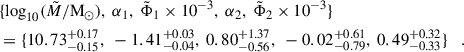
5.1. Fitting the MHI − M⋆ relation
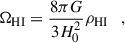
Figure 1 shows the resulting fit of the data points from Bianchetti et al. (2025) for the linear model (top panel) and polynomial model (bottom panel). We show the data from the combined stacking as blue squares and display the best-fit model to the data as a solid blue line. In addition, to check the consistency of the fit of the scaling relation, we also show the data from MIGHTEE and CHILES as well as the best-fitting models (MIGHTEE and CHILES).
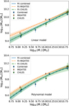 |
Fig. 1. MHI − M⋆ best-fitting scaling relations to the stacking results from Bianchetti et al. (2025). Top: Linear fit to the data. Bottom: Polynomial fit. The data points are shown as blue squares (combined stacking), green diamonds (MIGHTEE stacking), and green circles (CHILES stacking), and the best-fit models as solid blue (combined stacking), dashed orange (MIGHTEE stacking), and dotted-dashed green lines (CHILES stacking). |
When fitting the polynomial model to the combined case, we find that the free parameter c defined in Sect. 4.2 is not well constrained and consistent with zero. If we fix c = 0, we find that the best-fitting values for a and b remain unchanged, but the resulting uncertainties on both parameters are much smaller. Therefore, we decided to fix c = 0 for all the polynomial fits. This has two main advantages: (i) it lifts the parameter degeneracy discussed above, and (ii) it also enables a well-defined fit in the MIGHTEE and CHILES cases.
We report the best-fitting parameter values for both the linear and the polynomial model in Table 2. We leave blank the column of the values for a for the linear fit because the model does not have the second-order term, and the column of the values for c in the polynomial fit because we set c = 0, as discussed above.
From Fig. 1 we see that both the linear and the polynomial models provide reasonable fits to the data. We computed the reduced chi square, χ2/(degrees of freedom), and report the values in the last column of Table 2. Given the low number of degrees of freedom, it is hard to meaningfully establish which of the two models is preferred. Therefore, we decided to adopt as the fiducial model the polynomial one that, having a < 0, has the same qualitative properties as a double power law model (as anticipated in Sect. 4.2), i.e., it decreases more rapidly than a linear model toward low H I masses and flattens toward high H I masses.
5.2. The HI mass function and ΩHI at z ∼ 0.37
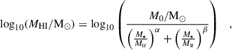
We fit a Schechter model to the resulting HIMF for the combined stacking and for both models for the MHI − M⋆ scaling relation (linear and polynomial) as described in Sect. 4.3. We report in Table 3 the results for the best-fitting values of the Schechter parameters  , as well as the resulting value for ΩHI computed as described in Sect. 4.3, together with a compilation of results from the literature. We report the results from the fitting of the HIMF resulting from MIGHTEE and CHILES stacking separately in Appendix A.
Figure 2 shows the resulting HIMF from this work (the linear model) and from the polynomial model. It also shows the best-fitting Schechter profiles as found from the median of the posterior distributions of the parameters and the results for the HIMF from the literature reported in Table 3. We show the results from ALFALFA at z ∼ 0 (Jones et al. 2018), MIGHTEE at 0 < z < 0.084 (Ponomareva et al. 2023), AUDS (Hoppmann et al. 2015) and BUDHIES (Gogate 2022) at z ∼ 0.16 and z ∼ 0.2, respectively (all based on direct detections), a HI intensity mapping experiment at z ∼ 0.32 (Paul et al. 2023), and the semiempirical HIMF results obtained by Bera et al. (2022) at z ∼ 0.35 and Chowdhury et al. (2024) at z ∼ 1 following similar approaches to the one adopted herein. We find a difference between the HIMF reported in this work and that at z ∼ 0 from ALFALFA. In particular, the HIMF derived here with both models have a consistently higher normalization than the ALFALFA HIMF, on average by a factor of ∼2. Compared to the MIGHTEE results at lower redshifts and to the AUDS survey at z ∼ 0.16, the HIMF from this work has a larger normalization at low MHI values, whereas they tend to converge toward high MHI. The results from BUDHIES, from Bera et al. (2022), and from Paul et al. (2023) have comparable normalization to the one of our results at low MHI, but they present a rapid fall-off toward high MHI, dropping below the ALFALFA HIMF at log10(M⋆/M⊙)≲9.6. Essentially, there is evidence of a variation between our results at z ∼ 0.37 and the results by Chowdhury et al. (2024) at z ∼ 1, the latter having a consistently larger normalization at the probed H I masses. These differences could be due to a potential evolution of the HIMF over cosmic time, or to possible selection biases or other systematics. The approach used in this work relies on a galaxy sample that is extracted from the COSMOS2020 catalog, and hence, selected in optical M⋆. This is not the case for, for example, blind H I surveys to which we are comparing our results. In general, the mentioned H I surveys feature a severe inhomogeneity in the covered area, depth and sensitivity, instrument and observational configuration (e.g., single dish vs. interferometric), among others. In addition, potential systematics related to the interferometric data from MIGHTEE and CHILES may also have an impact in the final results. Finally, as mentioned earlier in this section, the results on the HIMF to which we are comparing our findings are obtained following different methods. Therefore, given these aspects altogether, it is hard to conclusively tell if the detected differences between our results and the other tabulated results are fully due to cosmic evolution or are contaminated by the effects discussed above.
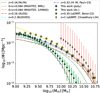 |
Fig. 2. Compilation of HIMF results from this work and from the literature. We show the resulting HIMF from the linear (yellow stars) and polynomial models (blue squares) as well as their best-fitting models as solid lines of the same color. We display the HIMFs from: ALFALFA at z ∼ 0 (Jones et al. 2018) as a dashed green line, MIGHTEE at 0 < z < 0.084 as dotted red (1/Vmax) and dotted-dashed gray (MML) lines (Ponomareva et al. 2023), AUDS at z ∼ 0.16 as a dotted-dashed brown line (Hoppmann et al. 2015), BUDHIES at z ∼ 0.2 as a dashed cyan line (Gogate 2022), the intensity mapping experiment at z ∼ 0.32 as a dotted-dashed purple line (Paul et al. 2023), and as green circles and orange diamonds the results from a similar approach as that followed here applied to stacking results from uGMRT data at z ∼ 0.35 (Bera et al. 2022) and z ∼ 1 (Chowdhury et al. 2024). |
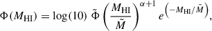
Figure 3 shows the results for ΩHI as a function of redshift derived in this work. We show the outcome from the combined stacking adopting a linear and polynomial model. In addition, we plot in the same figure a compilation of results from the literature. We notice that:
-
Our results are in broad agreement with other literature results at the same redshift, although the scatter in these results is large and encompasses values spanning an interval 0.35 × 10⁻³ ≲ ΩHI ≲ 0.95 × 10⁻³.
-
The linear model predicts consistently larger HIMF than the polynomial model. This translates into systematically larger values for ΩHI, as can be seen in Table 3.
-
The combined result adopting a polynomial model at z ∼ 0.37
 is compatible within 1σ with the results by MIGHTEE at 0 ≲ z ≲ 0.084, but deviates at ∼2.9σ from the value ΩHI = (3.90 ± 0.10)×10−3 reported by ALFALFA at z ∼ 0.
 -
The resulting values for ΩHI obtained by assuming the linear and the polynomial model for the scaling relation differ at ∼2.4σ for the combined stacking.
-
Our results for ΩHI follow the overall trend of ΩHI increasing with redshift.
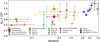 |
Fig. 3. Compilation of ΩHI results as a function of redshift from this work and from the literature: from this work, from the combined stacking with a linear model (yellow star) and with a polynomial model (red star); from ALFALFA at z ∼ 0 (blue diamond: Jones et al. 2018); from MIGHTEE at 0 < z < 0.084 with the 1/Vmax method (orange) and the MML method (green; Ponomareva et al. 2023); from a H I stacking based on WSRT data at z ∼ 0.066 (a red cross; Hu et al. 2019); from H I stacking on uGMRT data at z ∼ 0.35 (brown cross; Bera et al. 2019); from a H I intensity mapping experiment with MeerKAT (pink circle; Paul et al. 2023); from two H I stacking experiments based on uGMRT data at ∼0.32 (blue circle; Rhee et al. 2016) and z ∼ 0.37 (green circle; Rhee et al. 2016); from BUDHIES at ∼0.2 (green upward triangle; Gogate 2022); from H I stacking at z ∼ 0.24 based on GMRT data (cyan cross; Lah et al. 2007); from the cross-correlation between H I intensity mapping from the GBT and optical galaxies from the eBOSS survey (purple square; Wolz et al. 2022); from damped Lyα systems (DLAs) at z < 1.65 from (Rao et al. 2006, downward gray triangles) and (Rao et al. 2017, orange upward triangles); and from DLAs at z > 2 (dark blue squares; Noterdaeme et al. 2012) and at z > 4.4 (black diamonds; Crighton et al. 2015). |
5.3. Discussion
The main findings of this work point toward a difference in the HIMF and in the ΩHI parameters with respect to the fiducial ALFALFA HIMF at z ∼ 0. This fact is consistently inherited from the scaling relation from Bianchetti et al. (2025), which also features a clear deviation with respect to literature results at z ∼ 0. Assuming that the detected variations are due to actual evolution, and including the HIMF from Chowdhury et al. (2024) in the picture, the H I content of galaxies would evolve gradually and smoothly from z ∼ 0 to z ∼ 1. This scenario is in tension with the results from Bera et al. (2022) and from Paul et al. (2023). Both references promote a HIMF with similar normalization at log10(MHI/M⊙)∼9 − 9.5 as from this work, but with a quicker fall-off toward high MHI. This typically results in a lower value for ΩHI. In the case of Bera et al. (2022), the results is obtained with a similar approach as ours, but the authors therein used a different scaling relation to pass from MB to MHI. In addition, the sample size is a factor of ∼10 smaller than the one used in Bianchetti et al. (2025), so cosmic variance could be affecting at least partially the results when measuring H I masses from stacking. Eventually, the selection of star-forming galaxies performed by Bera et al. (2022) and Bianchetti et al. (2025) are based on different criteria based on colors. These aspects altogether may explain the observed differences, although we regard this comparison as not conclusive as in general more investigation with larger sample sizes is required. With respect to Paul et al. (2023), the HIMF obtained in that work are based on H I intensity mapping, i.e., a radically different approach from the one adopted herein. Therefore, it is difficult to establish a fair comparison in this case. Nonetheless, it is worth mentioning that the result obtained via H I intensity mapping is in good agreement with the HIMF obtained by Bera et al. (2022).
We notice that our results have a non-negligible dependence on the model adopted to describe the MHI − M⋆ relation. The linear model tends to produce HIMF with higher normalization and larger values for ΩHI than the polynomial model. This is not surprising since, as discussed, the polynomial model steepens toward low M⋆ where a greater number of galaxies is found. In addition, a linear model extrapolates the MHI − M⋆ relation to arbitrarily high value of MHI. However, results at z ∼ 0 show that massive galaxies feature a flattening in MHI at the high-mass end of the MHI − M⋆ relation, due to a plethora of phenomena shaping galaxy evolution, mainly gas depletion via star formation. In this work we find evidence that the polynomial model fits the data points from stacking better. The best-fitting second-order polynomial model for the MHI relation is found to have second-order coefficient a < 0 at a significance > 10σ in all the studied cases. While we regard this finding as nonconclusive given the limited amount of data points available for the fit, the trend suggested by the best-fitting polynomial fit qualitatively reproduces that described by a double power law at z ∼ 0 (Maddox et al. 2015; Parkash et al. 2018; Pan et al. 2023). The polynomial model with a < 0 accounts for the high-mass flattening of the MHI − M⋆ scaling relation. For all these reasons we regard the polynomial model as the fiducial model for this work.
5.4. Comparison with simulations
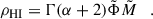
We also compared our findings to the predictions from publicly available cosmological hydrodynamic simulations, the SIMBA and IllustrisTNG simulations (previously described in Sect. 3), and constructed the HIMF for the different available models. For the SIMBA-50 simulation, we considered both the fiducial model and a number of alternatives varying the feedback model.
Figure 4 shows the detailed comparison of our results with the aforementioned simulations. We show in the top panel the global comparison with SIMBA and IllustrisTNG, while in the bottom panel we focus specifically on the different feedback model implemented in SIMBA. We also plot the HIMF from ALFALFA at z ∼ 0 for comparison.
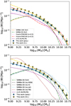 |
Fig. 4. Comparison of the HIMF from this work with the prediction from cosmological hydrodynamic simulations. Top: Comparison with the SIMBA full feedback model at z ∼ 0.365 and IllustrisTNG at z = 0.5. We show the HIMF determined in this work when assuming a linear (yellow stars) and polynomial model (blue squares) for the MHI − M⋆ relation. The best-fitting Schechter functions are shown with dashed orange and dotted-dashed green lines, respectively. We also show the predictions from SIMBA-100 (dashed yellow), SIMBA-50 (solid blue), IllustrisTNG-300 (dashed pink), and IllustrisTNG-100 (dotted-dashed red). For comparison, we show the HIMF from ALFALFA at z ∼ 0 (dashed purple). Bottom: Comparison with the different variations of the SIMBA-50 simulations. Shown are the predictions from the full feedback run (dashed green), the noAGN run (dotted black), the noX run (dashed gray), the noJet run (cyan line), and the noFB run (dotted brown). |
From the global comparison in the top panel, it turns out that there is no qualitative difference between the HIMF from SIMBA-50 and SIMBA-100. The incompleteness of the HIMF at log10(M⋆/M⊙)≲9.7 – stemming from the simulation resolution – is the main driver of the trend at low MHI, while no significant effects from cosmic variance are observed at high masses.
While at z = 0 both SIMBA and IllustrisTNG fit the ALFALFA HIMF well (Davé et al. 2020), neither reproduces our observations at z ∼ 0.37 very well at all the probed H I masses. SIMBA fits our HIMF well at the smallest H I masses at which the HIMF is complete, i.e., 9.75 ≲ log10(MHI/M⊙)≲10, but suffers a quick drop at higher H I masses, converging toward the HIMF at z ∼ 0 reported by ALFALFA. The high-mass end of the stellar and HIMF are known to be dominated by the effect of active galactic nucleus (AGN) feedback (e.g., Beckmann et al. 2017). Therefore, it is crucial to consider the effect of feedback, which is studied later on in this section.
IllustrisTNG-100 and IllustrisTNG-300 have different resolutions, which is reflected into the different completeness limit observable in the predicted HIMF. While IllustrisTNG-100 is found to be complete for all the probed H I masses (i.e., down to log10(MHI/M⊙)∼9), the lower-resolution IllustrisTNG-300 is found to become incomplete already at log10(MHI/M⊙)≲9.5. Because the values for MHI were computed by Diemer et al. (2018) using sub-grid recipes to split the atomic and molecular phases of neutral hydrogen, it is important to take into account that the different resolution is likely to have an important impact here on the prediction of the values for H I.
For both IllustrisTNG-100 and for IllustrisTNG-300 we observe a good convergence to our HIMF results at low MHI (the lowest masses at which each HIMF is complete). At high MHI, only IllustrisTNG-100 fits the HIMF from this work well, most likely due to resolution effects. At intermediate H I masses, none of them reproduces our HIMF; instead, they predict HIMFs that are more in agreement with the result at z ∼ 0 from ALFALFA.
In the bottom panel, we analyze the effect of the different implementations of feedback based on the SIMBA-50 run. As already mentioned, from the results shown in the top panel we observe that there are no obvious volume effects in the SIMBA runs, and hence, we can safely perform this study based on SIMBA-50, for which different versions with distinct feedback models have been produced. Specifically, we studied the following different cases:
-
full: the full SIMBA feedback model;
-
noAGN: the full AGN feedback model is not included;
-
noX: the X-ray AGN feedback model is not included;
-
noJet: the X-ray AGN and jet feedback models are not included;
-
noFB: no star formation nor AGN feedback models are included.
We started by observing that the noFB case clearly represents an unrealistic and oversimplified case. It produces a HIMF with an excess by a factor of ∼5.7 of low-MHI galaxies at log10(MHI/M⊙)∼9.3 with respect to the ALFALFA HIMF, and by a factor of ∼2.8 with respect to our HIMF, and a lack of high-MHI galaxies at log10(MHI/M⊙)∼10.35 by a factor of ∼3.6 with respect to ALFALFA and by a factor of ∼8.3 with respect to our results.
All the other feedback models converge well within each other and are in good agreement with our results at log10(MHI/M⊙)∼9.7, but tend to diverge toward high MHI values. The noX model underpredicts our results, the noAGN is in good agreement with them, and the noJet model overpredicts the HIMF. This indicates that, as expected, the specific AGN feedback model is a major driver of the massive end of the HIMF. It is particularly interesting to note that the noAGN model reproduces the HIMF from this work very well. The finding suggests a scenario in which neglecting the feedback from supermassive black holes enables a better modeling of the HIMF at the probed H I masses. This is consistent with the results from Gensior et al. (2023, 2024), where the authors considered tens of Milky-Way-like galaxies from the EMP-Pathfinder (Reina-Campos et al. 2022) and FIREbox (Feldmann et al. 2023) cosmological simulations and showed that they reproduce the observed H I properties of nearby galaxies well without the need of AGN feedback. Therefore, despite the large uncertainty associated with feedback models in current cosmological hydrodynamic simulations, we argue that a detailed study of these feedback mechanisms is crucial to properly understand which physical mechanism shapes the HIMF at the different H I masses.
6. Summary and conclusions
We report a novel indirect semiempirical estimation of the HIMF and the H I cosmic density parameter (ΩHI) for star-forming galaxies at z ∼ 0.37. We combined the most recent measurements of the stellar mass function of star-forming galaxies in the COSMOS field at 0.2 < z < 0.5 (Weaver et al. 2023) and of the MHI − M⋆ scaling relation of star-forming galaxies at 0.22 < z < 0.49 (median redshift of ∼0.37) by Bianchetti et al. (2025) from the combined H I stacking analysis of two state-of-the-art deep H I interferometric surveys, MIGHTEE (Jarvis et al. 2016) and CHILES (Fernández et al. 2013), both of which cover the COSMOS field. We adopted a Monte Carlo approach following that pioneered by Bera et al. (2022); it consists of drawing samples of the stellar mass function, generating a synthetic stellar mass sample from each stellar mass function, and converting M⋆ to MHI by assuming a MHI − M⋆ scaling relation with an adequate scatter. We computed the median and the standard deviation of the sample of HIMFs, which defines our “measured” HIMF. In addition, for each H I mass sample, we built the corresponding HIMF and fit a Schechter profile via a Markov chain Monte Carlo procedure using the emcee affine-invariant sampler (Foreman-Mackey et al. 2013). This allowed us to determine the full posterior distributions of the best-fitting Schechter parameters and, hence, to determine not only the median values but also their associated uncertainties after having adequately propagated all the uncertainties in our forward modeling.
The main findings of this paper can be summarized as follows:
-
We modeled the MHI − M⋆ scaling relation by fitting the data points from Bianchetti et al. (2025) using both a linear and a second-order polynomial model. The second-order coefficient (a) is found to be negative, a < 0. The resulting model resembles the well-known “curved trend” observed in the MHI − M⋆ relation at z = 0.
-
We find a global difference in the normalization of the HIMF from z ∼ 0 to z ∼ 1. The resulting HIMF from this work has a larger normalization than that reported by ALFALFA at z ∼ 0, and a smaller normalization than that reported by Chowdhury et al. (2024) at z ∼ 1. We tentatively interpret this as as a signature of the evolution of the HIMF, although it is hard to draw conclusions in this regard given the potential selection biases and systematics that could be affecting the comparison between our findings and the other literature results.
-
The linear model typically produces a HIMF with a larger normalization than the polynomial model.
-
The combined result when adopting a polynomial model at z ∼ 0.37
 is compatible within 1σ with the results by MIGHTEE at 0 ≲ z ≲ 0.084, but deviates at ∼2.9σ from the value ΩHI = (3.90 ± 0.10)×10−3 reported by ALFALFA at z ∼ 0.
 -
The resulting values for ΩHI obtained by assuming the linear and the polynomial model for the scaling relation differ by ∼2.4σ in the combined stacking case.
In conclusion, we argue that an approach similar to the one in this study can be used to derive the HIMF and the ΩHI parameter at different redshifts, provided that a reliable scaling relation is available to convert from well-studied mass and luminosity functions (such as those for M⋆ or MB) to MHI. In particular, future efforts at estimating, for example, the MHI − M⋆ scaling relation with larger samples will likely increase the number of available data points. This will help better constrain the functional form of such a relation and, hence, to increase the accuracy of the procedure.
Release 1, v2.2, March 2023.
We caution that the uncertainties on the MHI estimates, obtained via jackknife resampling by Bianchetti et al. (2025), refer to the error on the measurement and they do not represent the full underlying MHI distribution. The jackknife uncertainty typically underestimates the true dispersion.
Notice that the parametrization here is slightly different from the one used in Eq. (1). In Eq. (3) we use the same as in Ponomareva et al. (2023), while in Eq. (1) we use the one from Weaver et al. (2023) for consistency with their work.
We use Γ instead of γ to denote the incomplete Euler Gamma function for consistency with other references.
Acknowledgments
The authors warmly thank Nissim Kanekar, Apurba Bera and Aditya Chowdhury for providing the measurements underlying their publications. F.S. acknowledges the support of the Swiss National Science Foundation (SNSF) 200021_214990/1 grant. A.B. acknowledges the support of the doctoral grant funded by the University of Padova and by the Italian Ministry of Education, University and Research (MIUR). G.R. acknowledges the support from grant PRIN MIUR 2017- 20173ML3WW 001. A.B. and G.R. acknowledge support from INAF under the Large Grant 2022 funding scheme (project “MeerKAT and LOFAR Team up: a Unique Radio Window on Galaxy/AGN co-Evolution”). A.B. acknowledges financial support from the South African Department of Science and Innovation’s National Research Foundation under the ISARP RADIOMAP Joint Research Scheme (DSI-NRF Grant Number 150551), and from the Italian Ministry of Foreign Affairs and International Cooperation under the “Progetti di Grande Rilevanza” scheme (project RADIOMAP, grant number ZA23GR03). M.V. acknowledges financial support from the Inter-University Institute for Data Intensive Astronomy (IDIA), a partnership of the University of Cape Town, the University of Pretoria and the University of the Western Cape, and from the South African Department of Science and Innovation’s National Research Foundation under the ISARP RADIOSKY2020 and RADIOMAP Joint Research Schemes (DSI-NRF Grant Numbers 113121 and 150551) and the SRUG HIPPO Projects (DSI-NRF Grant Numbers 121291 and SRUG22031677).
References
- Arnouts, S., & Ilbert, O. 2011, Astrophysics Source Code Library [record ascl:1108.009] [Google Scholar]
- Bañares-Hernández, A., Castillo, A., Martin Camalich, J., & Iorio, G. 2023, A&A, 676, A63 [NASA ADS] [CrossRef] [EDP Sciences] [Google Scholar]
- Bauer, J. B., Marsh, D. J. E., Hložek, R., Padmanabhan, H., & Laguë, A. 2021, MNRAS, 500, 3162 [Google Scholar]
- Beckmann, R. S., Devriendt, J., Slyz, A., et al. 2017, MNRAS, 472, 949 [NASA ADS] [CrossRef] [Google Scholar]
- Bera, A., Kanekar, N., Chengalur, J. N., & Bagla, J. S. 2019, ApJ, 882, L7 [NASA ADS] [CrossRef] [Google Scholar]
- Bera, A., Kanekar, N., Chengalur, J. N., & Bagla, J. S. 2022, ApJ, 940, L10 [Google Scholar]
- Berti, M., Spinelli, M., & Viel, M. 2024, MNRAS, 529, 4803 [Google Scholar]
- Bianchetti, A., Sinigaglia, F., Rodighiero, G., et al. 2025, ApJ, 982, 82 [Google Scholar]
- Bigiel, F., Leroy, A., Walter, F., et al. 2008, AJ, 136, 2846 [NASA ADS] [CrossRef] [Google Scholar]
- Blitz, L., & Rosolowsky, E. 2006, ApJ, 650, 933 [NASA ADS] [CrossRef] [Google Scholar]
- Catinella, B., Saintonge, A., Janowiecki, S., et al. 2018, MNRAS, 476, 875 [NASA ADS] [CrossRef] [Google Scholar]
- Chang, T.-C., Pen, U.-L., Bandura, K., & Peterson, J. B. 2010, Nature, 466, 463 [Google Scholar]
- Chen, Z., Wolz, L., Spinelli, M., & Murray, S. G. 2021, MNRAS, 502, 5259 [Google Scholar]
- Chowdhury, A., Kanekar, N., & Chengalur, J. N. 2024, ApJ, 966, L39 [Google Scholar]
- Crighton, N. H. M., Murphy, M. T., Prochaska, J. X., et al. 2015, MNRAS, 452, 217 [Google Scholar]
- Cunnington, S., Li, Y., Santos, M. G., et al. 2023, MNRAS, 518, 6262 [Google Scholar]
- Davé, R., Thompson, R., & Hopkins, P. F. 2016, MNRAS, 462, 3265 [Google Scholar]
- Davé, R., Anglés-Alcázar, D., Narayanan, D., et al. 2019, MNRAS, 486, 2827 [Google Scholar]
- Davé, R., Crain, R. A., Stevens, A. R. H., et al. 2020, MNRAS, 497, 146 [Google Scholar]
- Davies, L. J. M., Robotham, A. S. G., Driver, S. P., et al. 2018, MNRAS, 480, 768 [NASA ADS] [CrossRef] [Google Scholar]
- DeBoer, D. R., Parsons, A. R., Aguirre, J. E., et al. 2017, PASP, 129, 045001 [NASA ADS] [CrossRef] [Google Scholar]
- Delhaize, J., Meyer, M. J., Staveley-Smith, L., & Boyle, B. J. 2013, MNRAS, 433, 1398 [NASA ADS] [CrossRef] [Google Scholar]
- DESI Collaboration (Adame, A. G., et al.) 2024, AJ, 168, 58 [NASA ADS] [CrossRef] [Google Scholar]
- Diemer, B., Stevens, A. R. H., Forbes, J. C., et al. 2018, ApJS, 238, 33 [NASA ADS] [CrossRef] [Google Scholar]
- Durbala, A., Finn, R. A., Crone Odekon, M., et al. 2020, AJ, 160, 271 [NASA ADS] [CrossRef] [Google Scholar]
- Feldmann, R., Quataert, E., Faucher-Giguère, C.-A., et al. 2023, MNRAS, 522, 3831 [NASA ADS] [CrossRef] [Google Scholar]
- Fernández, X., van Gorkom, J. H., Hess, K. M., et al. 2013, ApJ, 770, L29 [Google Scholar]
- Foreman-Mackey, D., Hogg, D. W., Lang, D., & Goodman, J. 2013, PASP, 125, 306 [Google Scholar]
- Galárraga-Espinosa, D., Aghanim, N., Langer, M., & Tanimura, H. 2021, A&A, 649, A117 [Google Scholar]
- Gensior, J., Feldmann, R., Mayer, L., et al. 2023, MNRAS, 518, L63 [Google Scholar]
- Gensior, J., Feldmann, R., Reina-Campos, M., et al. 2024, MNRAS, 531, 1158 [Google Scholar]
- Gnedin, N. Y., & Kravtsov, A. V. 2011, ApJ, 728, 88 [NASA ADS] [CrossRef] [Google Scholar]
- Gogate, A. 2022, Ph.D. Thesis, University of Groningen [Google Scholar]
- Hoppmann, L., Staveley-Smith, L., Freudling, W., et al. 2015, MNRAS, 452, 3726 [NASA ADS] [CrossRef] [Google Scholar]
- Hu, W., Hoppmann, L., Staveley-Smith, L., et al. 2019, MNRAS, 489, 1619 [NASA ADS] [CrossRef] [Google Scholar]
- Huang, S., Haynes, M. P., Giovanelli, R., & Brinchmann, J. 2012, ApJ, 756, 113 [Google Scholar]
- Ilbert, O., Arnouts, S., McCracken, H. J., et al. 2006, A&A, 457, 841 [NASA ADS] [CrossRef] [EDP Sciences] [Google Scholar]
- Jarvis, M., Taylor, R., Agudo, I., et al. 2016, in MeerKAT Science: On the Pathway to the SKA, 6 [Google Scholar]
- Jones, M. G., Haynes, M. P., Giovanelli, R., & Moorman, C. 2018, MNRAS, 477, 2 [Google Scholar]
- Khostovan, A. A., Kartaltepe, J. S., Salvato, M., et al. 2025, ArXiv e-prints [arXiv:2503.00120] [Google Scholar]
- Koopmans, L., Pritchard, J., Mellema, G., et al. 2015, in Advancing Astrophysics with the Square Kilometre Array (AASKA14), 1 [Google Scholar]
- Krumholz, M. R., & Gnedin, N. Y. 2011, ApJ, 729, 36 [Google Scholar]
- Lah, P., Chengalur, J. N., Briggs, F. H., et al. 2007, MNRAS, 376, 1357 [Google Scholar]
- Maddox, N., Hess, K. M., Obreschkow, D., Jarvis, M. J., & Blyth, S. L. 2015, MNRAS, 447, 1610 [Google Scholar]
- Maddox, N., Frank, B. S., Ponomareva, A. A., et al. 2021, A&A, 646, A35 [NASA ADS] [CrossRef] [EDP Sciences] [Google Scholar]
- Martin, A. M., Papastergis, E., Giovanelli, R., et al. 2010, ApJ, 723, 1359 [NASA ADS] [CrossRef] [Google Scholar]
- Martizzi, D., Vogelsberger, M., Artale, M. C., et al. 2019, MNRAS, 486, 3766 [Google Scholar]
- Masui, K. W., Switzer, E. R., Banavar, N., et al. 2013, ApJ, 763, L20 [Google Scholar]
- Jonas, J., & MeerKAT Team 2016, in MeerKAT Science: On the Pathway to the SKA, 1 [Google Scholar]
- Nelson, D., Pillepich, A., Genel, S., et al. 2015, Astron. Comput., 13, 12 [Google Scholar]
- Nelson, D., Springel, V., Pillepich, A., et al. 2019, Comput. Astrophys. Cosmol., 6, 2 [Google Scholar]
- Noterdaeme, P., Petitjean, P., Carithers, W. C., et al. 2012, A&A, 547, L1 [NASA ADS] [CrossRef] [EDP Sciences] [Google Scholar]
- O’Brien, J. G., Chiarelli, T. L., Dentico, J., et al. 2018, ApJ, 852, 6 [Google Scholar]
- Pan, H., Jarvis, M. J., Santos, M. G., et al. 2023, MNRAS, 525, 256 [NASA ADS] [Google Scholar]
- Parkash, V., Brown, M. J. I., Jarrett, T. H., & Bonne, N. J. 2018, ApJ, 864, 40 [NASA ADS] [CrossRef] [Google Scholar]
- Paul, S., Santos, M. G., Chen, Z., & Wolz, L. 2023, ArXiv e-prints [arXiv:2301.11943] [Google Scholar]
- Pinetti, E., Camera, S., Fornengo, N., & Regis, M. 2020, JCAP, 2020, 044 [Google Scholar]
- Ponomareva, A. A., Jarvis, M. J., Pan, H., et al. 2023, MNRAS, 522, 5308 [NASA ADS] [Google Scholar]
- Primack, J. R. 2024, Ann. Rev. Nucl. Part. Sci., 74, 173 [Google Scholar]
- Rao, S. M., Turnshek, D. A., & Nestor, D. B. 2006, ApJ, 636, 610 [Google Scholar]
- Rao, S. M., Turnshek, D. A., Sardane, G. M., & Monier, E. M. 2017, MNRAS, 471, 3428 [Google Scholar]
- Reina-Campos, M., Keller, B. W., Kruijssen, J. M. D., et al. 2022, MNRAS, 517, 3144 [NASA ADS] [CrossRef] [Google Scholar]
- Rhee, J., Lah, P., Chengalur, J. N., Briggs, F. H., & Colless, M. 2016, MNRAS, 460, 2675 [NASA ADS] [CrossRef] [Google Scholar]
- Rhee, J., Lah, P., Briggs, F. H., et al. 2018, MNRAS, 473, 1879 [NASA ADS] [CrossRef] [Google Scholar]
- Santos, M., Bull, P., Alonso, D., et al. 2015, in Advancing Astrophysics with the Square Kilometre Array (AASKA14), 19 [Google Scholar]
- Scoville, N., Aussel, H., Brusa, M., et al. 2007, ApJS, 172, 1 [Google Scholar]
- Sinigaglia, F., Kitaura, F.-S., Balaguera-Antolínez, A., et al. 2021, ApJ, 921, 66 [NASA ADS] [CrossRef] [Google Scholar]
- Sinigaglia, F., Rodighiero, G., Elson, E., et al. 2022, ApJ, 935, L13 [NASA ADS] [CrossRef] [Google Scholar]
- Sinigaglia, F., Rodighiero, G., Elson, E., et al. 2024, MNRAS, 529, 4192 [NASA ADS] [CrossRef] [Google Scholar]
- Somerville, R. S., & Davé, R. 2015, ARA&A, 53, 51 [Google Scholar]
- Springel, V. 2010, MNRAS, 401, 791 [Google Scholar]
- Sternberg, A., Le Petit, F., Roueff, E., & Le Bourlot, J. 2014, ApJ, 790, 10 [CrossRef] [Google Scholar]
- Vogelsberger, M., Marinacci, F., Torrey, P., & Puchwein, E. 2020, Nat. Rev. Phys., 2, 42 [Google Scholar]
- Weaver, J. R., Kauffmann, O. B., Ilbert, O., et al. 2022, ApJS, 258, 11 [NASA ADS] [CrossRef] [Google Scholar]
- Weaver, J. R., Davidzon, I., Toft, S., et al. 2023, A&A, 677, A184 [NASA ADS] [CrossRef] [EDP Sciences] [Google Scholar]
- Wolz, L., Pourtsidou, A., Masui, K. W., et al. 2022, MNRAS, 510, 3495 [NASA ADS] [CrossRef] [Google Scholar]
- Zhang, M., Li, Y., Zhang, J.-F., & Zhang, X. 2023, MNRAS, 524, 2420 [Google Scholar]
- Zwaan, M. A., Staveley-Smith, L., Koribalski, B. S., et al. 2003, AJ, 125, 2842 [Google Scholar]
Appendix A: Consistency of the HIMF from MIGHTEE and CHILES
In Sect. 5.2 we present the results obtained by assuming as fiducial case the combined stacking. Here, we test the consistency between such results and the ones separately from the MIGHTEE and CHILES surveys. Figure A.1 shows the resulting HIMF for the combined stacking, MIGHTEE, and CHILES for the linear and polynomial models for the MHI − M⋆ relation, along with the best-fit Schechter profiles, as well as the ALFALFA HIMF at z ∼ 0. We notice that the results from the three cases are always consistent within 1σ uncertainties. In addition, the uncertainties scale with the sample size, the combined case having the smallest and the CHILES case having the largest. This fact reflects that we are effectively incorporating the limited sample size in our framework and that taking it into account is an important piece of our modeling.
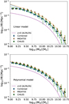 |
Fig. A.1. HIMF from the combined stacking (blue squares), MIGHTEE stacking (orange diamonds), and CHILES stacking (green circles). Top: HIMF results adopting the linear model for the MHI − M⋆ scaling relation. Bottom: HIMF results adopting the polynomial model for the MHI − M⋆ scaling relation. We also show the best-fitting Schechter models as solid blue, dashed orange, and dotted-dashed green lines, respectively. The ALFALFA HIMF at z ∼ 0 (dashed purple) is shown for comparison. |
As can be observed numerically from Table A.1, both for the linear and the polynomial models, MIGHTEE and CHILES predict the largest and the smallest values for ΩHI among the ones derived in this work, while the combined case yields an intermediate value for ΩHI between the other two, as expected from averaging the results from the two surveys. In addition, the MIGHTEE result obtained by using the polynomial model at z ∼ 0.37  is larger by ∼2.8σ than the values reported by MIGHTEE at 0 ≲ z ≲ 0.084
 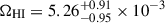 (1/Vmax method) and larger by ∼3.3σ for
 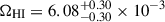 (modified maximum likelihood method, MML).
Numerical results for the best-fitting parameters to the HIMF using a Schechter model as in Eq. 3, for the results from the MIGHTEE, CHILES, and combined stacking.
The best-fitting values for the parameters of the Schechter model are always in agreement within 1σ in the combined, MIGHTEE, and CHILES cases. When comparing the results from the linear and the polynomial model, we report a systematic shift of  toward larger values and of α and
 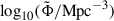 toward smaller values when passing from the linear to the polynomial model. While these shifts are not statistically significant and are often < 1σ, we observe them systematically for all the three cases. In addition, we show in Appendix F the posterior distributions for the different cases. Figures F.1 and F.2 show the resulting posterior distributions for the model parameters of the Schechter profile for the linear and the polynomial model, respectively. The distributions have qualitatively similar shapes, and the ones for CHILES are manifestly broader than the posteriors of the MIGHTEE and the combined cases, as expected from the smaller statistics. We take a closer look at the effect of the sample size in Appendix E. Figures F.3, F.4, and F.5 display a comparison between the posterior distributions from the linear (solid blue) and the polynomial model (dashed orange), for the combined, MIGHTEE, and CHILES cases, respectively. Here, we clearly appreciate the systematic shift of the posteriors when passing from the linear to the polynomial model.
Appendix B: The impact of scatter
As shown by Bera et al. (2022), properly modeling the scatter of the scaling relation used to derive the final HI mass sample is of pivotal importance to correctly reproduce the final HIMF. Bera et al. (2022) found that assuming zero scatter on the MHI − MB relation used to convert from MB to MHI severely underestimates the massive end of the ALFALFA HIMF at z ∼ 0. Here, we built upon that experiment and applied the full forward model assuming different values for the scatter: σ = {0, 0.1, 0.2, 0.3, 0.4, 0.5} dex. We show the resulting HIMF in Fig. B.1. One immediately sees that the HIMF is indeed very sensitive to the assumed scatter, with the high-mass end of the HIMF increasing to larger values with increasing scatter. This is due to the fact that the scatter allows us to sample synthetic MHI values from a statistical distribution at fixed M⋆, instead of having a deterministic estimate. In terms of HIMF, this translates in a higher probability of generating low- and high-MHI galaxies the larger the scatter. This test shows the importance of carefully modeling the scatter and assuming an adequate value for it.
In addition, after choosing σ = 0.39 as motivated by z ∼ 0 results from the xGASS survey (Catinella et al. 2018) and explained in Sect. 4.2, we also incorporated into our analysis an additional source of error coming from the intrinsic uncertainty on the true value of the scatter. For each step of our Monte Carlo approach, we added to the scatter a random error sampled from a Gaussian distribution with zero mean and standard deviation σerr = 0.05. In this way, we forward-modeled this additional source of uncertainty and propagated it throughout the whole procedure. We report In Table B.1 the results of the best-fitting parameters to the HIMF for the Schechter function, with and without assuming the uncertainty on the scatter. As can be seen from the numerical results, the differences between including or not the scatter are negligible and not systematic. Specifically, the uncertainties on the best-fitting parameters remain roughly unchanged, and the median values suffer tiny random shifts, which are not statistically significant. As explained in Sect. 4.2, we hence assumed as the fiducial methodology the one that includes the error on the scatter, for completeness.
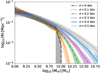 |
Fig. B.1. HIMF results from the combined stacking case as a function of the assumed scatter in the MHI − M⋆ and for the polynomial model. We show the results for σ = 0 (dotted-dashed black) σ = 0.1 (dashed orange), σ = 0.2 (dotted-dashed green), σ = 0.3 (dotted purple), σ = 0.4 (solid blue), and σ = 0.5 (dashed gray). Bottom: HIMF from the combined stacking assuming a polynomial and an asymmetric scattering (orange diamonds), compared to the fiducial HIMF from this work (blue squares) and the ALFALFA HIMF at z ∼ 0 (dashed green). |
Best-fit parameters of the HIMF with and without assuming the uncertainty on the scatter.
Appendix C: The impact of the MHI distribution asymmetry
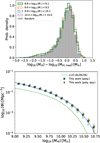 |
Fig. C.1. Results of testing the impact of an asymmetric scatter for the MHI − M⋆ relation. Top: MHI distributions (from which we have subtracted the median) in different stellar mass bins: 8.9 < log10(M⋆/M⊙) < 9.1 (solid green), 9.4 < log10(M⋆/M⊙) < 9.6 (dashed orange), 9.9 < log10(M⋆/M⊙) < 10.1 (dotted-dashed blue), and 10.4 < log10(M⋆/M⊙) < 10.5 (dotted purple). In dashed gray we show a lognormal random distribution obtained by assuming σ = 0.45, which is found to approximate all the MHI distributions well. |
Throughout the main analysis underlying this paper, we assumed that the MHI distribution at fixed stellar mass is symmetric in log space, and we modeled the scatter by sampling MHI values from a Gaussian distribution. In this appendix we relax this assumption and test the impact of assuming an asymmetric distribution instead.
To do so, we first considered the cross-matched ALFALFA-SDSS catalog (Durbala et al. 2020), notably the MHI distribution in different stellar mass bins. We display the results (from which we have subtracted the median, to have them centered in zero) in the top panel of Fig. C.1. A visual inspection of such distributions reveals that they are manifestly asymmetric, with the lower envelope featuring a larger dispersion (σ ∼ 0.5 dex) than the upper envelope (σ ∼ 0.38 dex). We also observe that the MHI histograms are almost independent of stellar mass. We find that a lognormal distribution with σ = 0.45 (dashed gray) represents all the different MHI distributions well. Therefore, we repeated the main analysis but replacing the Gaussian scatter with a lognormal scatter (in log space) as described above. We display the resulting HIMF (orange diamonds) in the bottom panel of Fig. C.1, compared to the results from assuming a Gaussian scatter (blue squares) and to the HIMF from ALFALFA at z ∼ 0 for comparison. The outcome of this experiment highlights that the difference between assuming appropriate symmetric and asymmetric scatters is negligible in this case. Therefore, assuming a Gaussian scatter, even though simplistic, turns out to be a robust assumption in our framework.
Appendix D: Completeness effects on the HIMF
Figure D.1 shows the resulting HIMF from assuming the combined scaling relation and the linear (yellow stars) and the polynomial (blue squares) models. The HIMF presents evidence of incompleteness at log10(MHI/M⊙)≲9. As stated in Sect. 4.3, we conservatively fit the Schechter model only at log10(MHI/M⊙) > 9.2 for the polynomial model and at log10(MHI/M⊙) > 9.4 for the linear model. The MHI lower limits for the fit, log10(MHI/M⊙) = 9.2 and log10(MHI/M⊙) = 9.4, are marked. We also display the best-fitting Schechter models obtained adopting the fitting strategy outlined above.
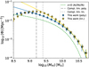 |
Fig. D.1. Completeness effects on the HIMFs obtained by assuming the linear (yellow stars) and the polynomial (blue squares) models for the MHI − M⋆ relation. The vertical dashed and dotted gray lines stand for the conservative completeness limits log10(MHI/M⊙) = 9.2 and log10(MHI/M⊙) = 9.4 for the polynomial and linear cases, respectively, and represent the lower limits used for the fit of the Schechter models to the data. We show the best-fitting Schechter models obtained by adopting the fitting strategy outlined above as solid yellow (linear model) and solid blue (polynomial model). We also display the HIMF from ALFALFA at z ∼ 0 (dashed green) for comparison. |
Appendix E: The impact of sample size
To assess the impact of the assumed sample size, we repeated the main procedure outlined in Sect. 4 but varying the sample size. Doing so, we aimed to test the impact on the HIMF of the sample size, which we matched to that used in the analysis from Bianchetti et al. (2025). Figure E.1 shows the results of this test: we compare the results for the combined stacking case from the "true" sample size presented in Sect. 5.2 (blue squares) with the resulting HIMF from increasingly larger samples of N sizes. One sees that there are no evident systematic effects due to sample size for N > 1000. Only in the case N = 100 and N = 1000 is a small systematic shift of the HIMF observed, although it is well within the uncertainties. For N = 100 the HIMF is not measured for the used binning and setup at log10(MHI/M⊙)≳10.2 due to an insufficient sampling.
This test has two important implications for this work. First, it is safe to assume that for the sample sizes used in our experiment, the results are well converged, and the sample size only affects the magnitude of the uncertainty, as sought. Second, given the large uncertainties featured by the cases N = 100 and N = 1000, it is not surprising that current results from the literature building the HIMF with a few tens or hundreds of H I detections are not well converged.
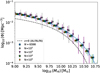 |
Fig. E.1. Results for the HIMF from the combined stacking case as a function of the chosen sample size (N) and assuming the polynomial model for the MHI − M⋆ relation. We show the main results from this paper: N = 6598 (blue squares), N = 102 (gray circles), N = 103 (purple downward triangles), N = 104 (green stars), and N = 105 (orange diamonds). We also display the HIMF from ALFALFA at z ∼ 0 as a dashed black line for comparison. A tiny horizontal shift was applied to the data points to avoid overlaps and to ease visualization. |
Appendix F: Posterior distributions of the model parameters
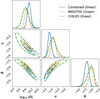 |
Fig. F.1. Posterior distributions of the best-fitting parameters of the Schechter profile to the HIMF when assuming a linear model for the MHI − M⋆ relation. The contours represent the 68% and 99% confidence levels. |
In this appendix we display the posterior distributions for the different studied cases. Figures F.1 and F.2 show the resulting posterior distributions for the model parameters of the Schechter profile for the linear and the polynomial model, respectively. Figures F.3, F.4, and F.5 display instead a comparison between the posterior distributions from the linear and the polynomial model for the combined, MIGHTEE, and CHILES cases. Here, we clearly appreciate the systematic shift of the posteriors when passing from the linear to the polynomial model.
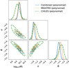 |
Fig. F.2. Same as Fig. F.1 but when assuming a polynomial model. |
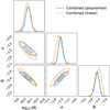 |
Fig. F.3. Same as Fig. F.1 but for the combined stacking case. |
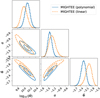 |
Fig. F.4. Same as Fig. F.1 but for the MIGHTEE stacking case. |
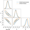 |
Fig. F.5. Same as Fig. F.1 but for the CHILES stacking case. |
All Tables
Numerical results for the best-fitting parameters to the HIMF using a Schechter model as in Eq. 3, for the results from the MIGHTEE, CHILES, and combined stacking.
Best-fit parameters of the HIMF with and without assuming the uncertainty on the scatter.
All Figures
|
Fig. 1. MHI − M⋆ best-fitting scaling relations to the stacking results from Bianchetti et al. (2025). Top: Linear fit to the data. Bottom: Polynomial fit. The data points are shown as blue squares (combined stacking), green diamonds (MIGHTEE stacking), and green circles (CHILES stacking), and the best-fit models as solid blue (combined stacking), dashed orange (MIGHTEE stacking), and dotted-dashed green lines (CHILES stacking). |
| In the text | |
|
Fig. 2. Compilation of HIMF results from this work and from the literature. We show the resulting HIMF from the linear (yellow stars) and polynomial models (blue squares) as well as their best-fitting models as solid lines of the same color. We display the HIMFs from: ALFALFA at z ∼ 0 (Jones et al. 2018) as a dashed green line, MIGHTEE at 0 < z < 0.084 as dotted red (1/Vmax) and dotted-dashed gray (MML) lines (Ponomareva et al. 2023), AUDS at z ∼ 0.16 as a dotted-dashed brown line (Hoppmann et al. 2015), BUDHIES at z ∼ 0.2 as a dashed cyan line (Gogate 2022), the intensity mapping experiment at z ∼ 0.32 as a dotted-dashed purple line (Paul et al. 2023), and as green circles and orange diamonds the results from a similar approach as that followed here applied to stacking results from uGMRT data at z ∼ 0.35 (Bera et al. 2022) and z ∼ 1 (Chowdhury et al. 2024). |
| In the text | |
|
Fig. 3. Compilation of ΩHI results as a function of redshift from this work and from the literature: from this work, from the combined stacking with a linear model (yellow star) and with a polynomial model (red star); from ALFALFA at z ∼ 0 (blue diamond: Jones et al. 2018); from MIGHTEE at 0 < z < 0.084 with the 1/Vmax method (orange) and the MML method (green; Ponomareva et al. 2023); from a H I stacking based on WSRT data at z ∼ 0.066 (a red cross; Hu et al. 2019); from H I stacking on uGMRT data at z ∼ 0.35 (brown cross; Bera et al. 2019); from a H I intensity mapping experiment with MeerKAT (pink circle; Paul et al. 2023); from two H I stacking experiments based on uGMRT data at ∼0.32 (blue circle; Rhee et al. 2016) and z ∼ 0.37 (green circle; Rhee et al. 2016); from BUDHIES at ∼0.2 (green upward triangle; Gogate 2022); from H I stacking at z ∼ 0.24 based on GMRT data (cyan cross; Lah et al. 2007); from the cross-correlation between H I intensity mapping from the GBT and optical galaxies from the eBOSS survey (purple square; Wolz et al. 2022); from damped Lyα systems (DLAs) at z < 1.65 from (Rao et al. 2006, downward gray triangles) and (Rao et al. 2017, orange upward triangles); and from DLAs at z > 2 (dark blue squares; Noterdaeme et al. 2012) and at z > 4.4 (black diamonds; Crighton et al. 2015). |
| In the text | |
|
Fig. 4. Comparison of the HIMF from this work with the prediction from cosmological hydrodynamic simulations. Top: Comparison with the SIMBA full feedback model at z ∼ 0.365 and IllustrisTNG at z = 0.5. We show the HIMF determined in this work when assuming a linear (yellow stars) and polynomial model (blue squares) for the MHI − M⋆ relation. The best-fitting Schechter functions are shown with dashed orange and dotted-dashed green lines, respectively. We also show the predictions from SIMBA-100 (dashed yellow), SIMBA-50 (solid blue), IllustrisTNG-300 (dashed pink), and IllustrisTNG-100 (dotted-dashed red). For comparison, we show the HIMF from ALFALFA at z ∼ 0 (dashed purple). Bottom: Comparison with the different variations of the SIMBA-50 simulations. Shown are the predictions from the full feedback run (dashed green), the noAGN run (dotted black), the noX run (dashed gray), the noJet run (cyan line), and the noFB run (dotted brown). |
| In the text | |
|
Fig. A.1. HIMF from the combined stacking (blue squares), MIGHTEE stacking (orange diamonds), and CHILES stacking (green circles). Top: HIMF results adopting the linear model for the MHI − M⋆ scaling relation. Bottom: HIMF results adopting the polynomial model for the MHI − M⋆ scaling relation. We also show the best-fitting Schechter models as solid blue, dashed orange, and dotted-dashed green lines, respectively. The ALFALFA HIMF at z ∼ 0 (dashed purple) is shown for comparison. |
| In the text | |
|
Fig. B.1. HIMF results from the combined stacking case as a function of the assumed scatter in the MHI − M⋆ and for the polynomial model. We show the results for σ = 0 (dotted-dashed black) σ = 0.1 (dashed orange), σ = 0.2 (dotted-dashed green), σ = 0.3 (dotted purple), σ = 0.4 (solid blue), and σ = 0.5 (dashed gray). Bottom: HIMF from the combined stacking assuming a polynomial and an asymmetric scattering (orange diamonds), compared to the fiducial HIMF from this work (blue squares) and the ALFALFA HIMF at z ∼ 0 (dashed green). |
| In the text | |
|
Fig. C.1. Results of testing the impact of an asymmetric scatter for the MHI − M⋆ relation. Top: MHI distributions (from which we have subtracted the median) in different stellar mass bins: 8.9 < log10(M⋆/M⊙) < 9.1 (solid green), 9.4 < log10(M⋆/M⊙) < 9.6 (dashed orange), 9.9 < log10(M⋆/M⊙) < 10.1 (dotted-dashed blue), and 10.4 < log10(M⋆/M⊙) < 10.5 (dotted purple). In dashed gray we show a lognormal random distribution obtained by assuming σ = 0.45, which is found to approximate all the MHI distributions well. |
| In the text | |
|
Fig. D.1. Completeness effects on the HIMFs obtained by assuming the linear (yellow stars) and the polynomial (blue squares) models for the MHI − M⋆ relation. The vertical dashed and dotted gray lines stand for the conservative completeness limits log10(MHI/M⊙) = 9.2 and log10(MHI/M⊙) = 9.4 for the polynomial and linear cases, respectively, and represent the lower limits used for the fit of the Schechter models to the data. We show the best-fitting Schechter models obtained by adopting the fitting strategy outlined above as solid yellow (linear model) and solid blue (polynomial model). We also display the HIMF from ALFALFA at z ∼ 0 (dashed green) for comparison. |
| In the text | |
|
Fig. E.1. Results for the HIMF from the combined stacking case as a function of the chosen sample size (N) and assuming the polynomial model for the MHI − M⋆ relation. We show the main results from this paper: N = 6598 (blue squares), N = 102 (gray circles), N = 103 (purple downward triangles), N = 104 (green stars), and N = 105 (orange diamonds). We also display the HIMF from ALFALFA at z ∼ 0 as a dashed black line for comparison. A tiny horizontal shift was applied to the data points to avoid overlaps and to ease visualization. |
| In the text | |
|
Fig. F.1. Posterior distributions of the best-fitting parameters of the Schechter profile to the HIMF when assuming a linear model for the MHI − M⋆ relation. The contours represent the 68% and 99% confidence levels. |
| In the text | |
|
Fig. F.2. Same as Fig. F.1 but when assuming a polynomial model. |
| In the text | |
|
Fig. F.3. Same as Fig. F.1 but for the combined stacking case. |
| In the text | |
|
Fig. F.4. Same as Fig. F.1 but for the MIGHTEE stacking case. |
| In the text | |
|
Fig. F.5. Same as Fig. F.1 but for the CHILES stacking case. |
| In the text | |
Current usage metrics show cumulative count of Article Views (full-text article views including HTML views, PDF and ePub downloads, according to the available data) and Abstracts Views on Vision4Press platform.
Data correspond to usage on the plateform after 2015. The current usage metrics is available 48-96 hours after online publication and is updated daily on week days.
Initial download of the metrics may take a while.