| Issue |
A&A
Volume 704, December 2025
|
|
|---|---|---|
| Article Number | A229 | |
| Number of page(s) | 15 | |
| Section | Stellar atmospheres | |
| DOI | https://doi.org/10.1051/0004-6361/202556230 | |
| Published online | 16 December 2025 | |
PENELLOPE
VIII. Veiling and extinction variations of V505 Ori★
1
Thüringer Landessternwarte Tautenburg,
Sternwarte 5,
07778
Tautenburg,
Germany
2
Hamburger Sternwarte, Universität Hamburg,
Gojenbergsweg 112,
21029
Hamburg,
Germany
3
Institut für Theoretische Physik und Astrophysik, Christian-Albrechts-Universität zu Kiel,
Leibnizstraße 15,
24118
Kiel,
Germany
4
Centre for Astrophysics and Planetary Science, School of Physics and Astronomy, University of Kent,
Canterbury
CT2 7NH,
UK
5
Institut für Astronomie und Astrophysik, Eberhard Karls Universität Tübingen,
Sand 1,
72076
Tübingen,
Germany
6
INAF—Osservatorio Astrofisico di Catania,
via S. Sofia 78,
95123
Catania,
Italy
7
European Southern Observatory,
Karl-Schwarzschild-Strasse 2,
85748
Garching bei München,
Germany
★★ Corresponding author: bfuhrmeister@tls-tautenburg.de
Received:
3
July
2025
Accepted:
4
November
2025
Disk warps and accretion hot spots may leave their imprint on photometric light curves and spectra of TTauri stars. We disentangle accretion and extinction signatures for the V505 Ori system using photometry in the B, V, R, and I bands taken mainly between November 2019 and November 2024, three ESO VLT/UVES spectra from November and December 2020, and two ESO/X-Shooter spectra taken in February and December 2020. V505 Ori has tentatively been classified as an AA Tau-like dipper based on photometric light curves. With the three UVES spectra and one X-Shooter spectrum taken from one brightness maximum to the next minimum, we find decreasing veiling with r500=2.22 ± 0.29 to 1.06 ± 0.32 and increasing reddening from AV=0.0 to 0.85 mag from maximum to minimum (optical) brightness. From the spectra we also report accretion features around the brightness maximum that contrast with the behaviour of AA Tau-like dippers, which show such features at the brightness minimum. For V505 Ori we therefore propose a scenario with a hot circumpolar accretion spot in combination with a more severe occultation by the stellar disk at brightness minimum. From photometric and spectral model fitting, we infer accretion spot sizes of about 10–20% at the brightness maximum down to 5% at the brightness minimum. Moreover, the spectral model fitting allows us to estimate that up to about 80% of the stellar light is blocked by the disk, while about 50% down to 10% of the stellar disk light is subject to reddening as its line of sight passes through outer layers of the disk. Moreover, there must be long-term variability of the accretion flow, as evidenced by the X-Shooter spectrum taken 10 months earlier.
Key words: stars: late-type / stars: individual: V505 Ori / stars: pre-main sequence
© The Authors 2025
 Open Access article, published by EDP Sciences, under the terms of the Creative Commons Attribution License (https://creativecommons.org/licenses/by/4.0), which permits unrestricted use, distribution, and reproduction in any medium, provided the original work is properly cited.
This article is published in open access under the Subscribe to Open model. Subscribe to A&A to support open access publication.
1 Introduction
The formation of low-mass stars can be divided into several phases. Thereof, the so-called classical TTauri star (CTTS) phase is perhaps the most intriguing and most studied. During this phase, the young star exhibits strong magnetic fields, accretes matter from an accretion disk, and may harbour disk winds (Hartmann et al. 2016). Accretion is thought to be funnelled by the stellar magnetic fields to build accretion shocks at the stellar surface, which result in emission lines in the spectrum from the hot plasma in the funnels and the shock region. Additionally, the shocked plasma emits a continuum that fills in the photospheric absorption lines (an effect called veiling; see e.g. Hartigan et al. 1989).
One characteristic feature of CTTSs is the variability in their photometric light curves (Joy 1945; Alencar et al. 2010; Cody et al. 2014; Venuti et al. 2021; Fischer et al. 2023, 2024). Cody et al. (2014) developed a classification scheme based on stochasticity and flux asymmetry. One of their categories contains stars with stochastically or periodically occurring dimming events, so-called dippers. A typical (quasi-)periodic dipper is AA Tau, which exhibits an about flat top photometric light curve with dimming events lasting more than half of the period and exhibiting differences in depth and shape for each period. The periodicity of AA Tau is about eight days, and the dimming has been interpreted as an occultation event of a warped disk for this system seen nearly edge-on (Bouvier et al. 1999). Bouvier et al. (2007) analysed spectroscopic data of AA Tau during the course of the dimming and found that at the photometric minimum, accretion features (i.e. veiling and He I flux) are strongest, which indicates that the inner disk wall and the accretion spot are located at the same rotational phase. For the same phase they found red-shifted absorption features in the broad Hα line as a direct imprint of the accretion funnel being in the line of sight. A very similar behaviour has been shown by the transition disk object LK Ca 15 (Alencar et al. 2018).
Another category in the classification scheme by Cody et al. (2014) is the quasi-periodic symmetric light curves, which may be explained by dark or bright spots showing some intrinsic variation (by fast spot evolution or changes in accretion) or a modulation with longer timescale aperiodic changes (in accretion). They may even be caused by some structures rotating with the accretion disk (Cody et al. 2013).
In this work, we analyse the quasi-periodic brightness variations of V505 Ori by making use of high-resolution spectra taken in the descending part of the light curve. We want to shed light on the accretion geometry of the system and especially seek to ascertain if the variability is caused by occultation events (dipper class), spots on the stellar surface, or a combination thereof.
Our paper is structured as follows: In Sect. 2 we describe previous work on V505 Ori, and in Sect. 3 we give a short description of the archival data we used and our calibration of the data. We determine the veiling in Sect. 4 and the extinction in Sect. 5. We revisit the photometry data in Sect. 6, and we state our results about the emission lines in Sect. 7. We discuss possible scenarios in Sect. 8 and present our conclusions in Sect. 9.
Stellar parameters taken from the literature and derived from the data used here.
2 Previous work on V505 Ori
V505 Ori (also called SO518 in many studies) is located in the σ Orionis star forming cluster, which has an age of about 3–5 Myr (Oliveira et al. 2004). Its spectral type is K6 or K7, and measurements of the effective temperature vary between about 4000 and 4400 K. An overview of the stellar parameters of V505 Ori selected from the literature can be found in Table 1. The extinction values range from AV = 0.0 to 1.6 mag for different datasets, suggesting a variable AV, which we also want to investigate further. Gangi et al. (2023) proposed a high inclination of about i = 80°, which was inferred from unresolved spectral energy distribution disk modelling (Maucó et al. 2018) and thus refers to the outer disk. Moreover, the reddening towards the centre of the cluster was observed to be low (Hernández et al. 2014), so significant extinction is probably caused within the star-disk system.
V505 Ori was found to show photometric variability with a period of 7 days (Froebrich et al. 2022). The light curve exhibits periodicity in all photometric filters with a triangular shaped minimum and a rounded maximum and a scatter in amplitude of as much as one magnitude especially around the minima. The periodic variation can be explained either by star spots or V505 Ori being an AA Tau-like object. Froebrich et al. (2022) calculated a suite of one-spot models and found that none of these models represents the light curve well. However, they also caution that if variations are caused by an occulting structure in the accretion disk, the structure has to be asymmetric due to the triangular shape of the minima (e.g. sharp trailing edge), and that the variations in the amplitude of the light curve indicate a variation of the column depth in the line of sight by a factor of about two.
3 Data
3.1 Photometry
We made use of the photometry data for V505 Ori from the Hunting Outbursting Young Stars (HOYS) project (Froebrich et al. 2018). This is a citizen science project that collects images from amateur astronomers for a number of nearby star forming regions, including σOrionis. For all HOYS images relative photometry is performed, including the correction of colour terms, with respect to deep reference frames taken in U, B, V, Rc, and Ic filters (Froebrich et al. 2018; Evitts et al. 2020). We have obtained 27 U, 1876 B, 2401 V, 2439 Rc, and 2228 Ic data points for V505 Ori, taken between JD=2458115.53 and JD=2460707.45 d (December 2017 to January 2025).
Additionally, we used B, V, Rc, and Ic band data from the American Association of Variable Star Observers (AAVSO) international database1, which is the most comprehensive digital variable star database in the world consisting of mostly amateur made observations (Percy & Mattei 1993). We downloaded 2192 B band, 3169 V and Rc band, and 2226 Ic band observations for V505 Ori taken between JD=2458808.46 and 2460643.23 d (November 2019 to November 2024).
While the data of both archives are consistent within their nominal measurement uncertainties in the B and V filters, we noticed a slight offset between HOYS and AAVSO data in the Rc filter of about 0.25 mag and a larger one in the Ic filter of about 0.42 mag. To decide for the correct magnitudes, we use further data from the Serra La Nave observatory of Osservatorio Astrofisico di Catania (OACt), which exists for a smaller time baseline between JD=2459179 and JD=2459200 d. These data were taken in broadband Bessel filters (B, V, R, I, Z) and during the data reduction transformed to the Johnson-Cousin system. They were already published and described in Manara et al. (2021) and are in agreement with the AAVSO R and I band data. Therefore, we corrected the HOYS data to match the AAVSO data. A subset of the data around the spectral observations is shown in Fig. 1.
To complement the ground-based photometry, we analysed space-based observations of V505 Ori obtained by the Transiting Exoplanet Survey Satellite (TESS, see Ricker et al. 2015). The target was observed during Sector 6 (2018-12-11 to 2019-01-07) and Sector 32 (2020-11-19 to 2020-12-17). We extracted the light curves using the Quick Look Pipeline (QLP; Feinstein et al. 2020), which is optimised for bright stars in the Full Frame Images (FFIs). The QLP provides 30-minute cadence light curves corrected for common instrumental systematics and crowding, making them well suited for variability studies.
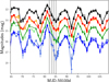 |
Fig. 1 Photometric data around the spectroscopic observations. The different photometric bands are B (blue – HOYS, light blue – AAVSO), V (green – HOYS, light greeen – AAVSO), Rc (red – HOYS, orange – AAVSO), and Ic (black – HOYS, grey – AAVSO). The HOYS R and I band have been shifted by +0.25 and +0.42 mag, respectively, to match the AAVSO data. The vertical grey lines mark the UVES (first three) and X-Shooter (last one) observations. |
3.2 Spectroscopy
We used archival spectra taken in the framework of the PENELLOPE programme, which is an ESO Large programme that complements the Hubble Space Telescope (HST) UV Legacy Library of Young Stars (ULLYSES; Roman-Duval et al. 2020). The PENELLOPE survey was described in Manara et al. (2021) including observational strategy, data reduction, and data analysis accomplished for all program stars in the Orion OB1 association and in the σ Orionis cluster. V505 Ori (identified as SO 518 in Manara et al. 2021) was observed with the ultraviolet and visual Echelle spectrograph (UVES) at VLT/ESO in three nights (2020-11-29, 2020-11-30, and 2020-12-01) with a spectral resolution of R~70 000 for the blue and the red arm of the spectra with a wavelength coverage from ~3300–4500 Å and 4800–6800 Å, respectively. We call these the UVES spectra no. 1–3. Furthermore, V505 Ori was observed on 2020-12-02 with the X-Shooter instrument, which provides spectra with three arms with a much larger wavelength coverage of 3000–5000 Å (UVB, R~5400), 5000–10 000 Å (VIS, R~18 400), and 10 000–25 000 Å (NIR, R~11 600). We call this the X-Shooter spectrum no. 1. Moreover, we used an additional X-Shooter spectrum taken on 2020-02-07 under programme ID 0104.C-0454(A). This was published already by Maucó et al. (2023), where the data reduction is described. We use their reduced spectrum here and call this the X-Shooter spectrum no. 2.
Since the data reduction is described in detail in Manara et al. (2021) and Maucó et al. (2023) we only mention here, that the X-Shooter spectrum no. 2 was taken under clear conditions, while the PENELLOPE spectra were taken under photometric conditions. All data had telluric lines removed using Molecfit (Smette et al. 2015). Both X-Shooter observations have been complemented with wide slit observations for absolute flux calibration.
While for UVES spectrum no. 1–3 and X-Shooter spectrum no. 1 the phase in the brightness cycle can be inferred from (quasi-)simultaneous photometry (cf. Fig. 1), the case is more complicated for X-Shooter spectrum no. 2. Since the coverage by photometry is much sparser at this time compared to later times when the PENELLOPE observations where performed, we used phase-folded light curves to determine the phase of the photometric measurement near the X-Shooter no. 2 observation. Froebrich et al. (2022) found a period of 7.070 ± 0.007 d using periodogram analysis in the different filters. We combined the HOYS and AAVSO data in the different filters and computed a generalised Lomb-Scargle periodogram (Ferraz-Mello 1981; Zechmeister & Kürster 2009). Taking the mean and standard deviation of these measurements (from the four filters) leads to a period of 7.0814 ± 0.0004. Interpolating this period to the time of the observation of the X-Shooter no. 2 spectrum, allowed us to infer that it was taken during brightness decay at a time in the dipper cycle similar to the UVES no. 2 spectrum as shown in Fig. 2.
3.3 Archival template and model spectra
For the veiling calculations we used as template the K6 main sequence star HD 200779 (Teff = 4406 K, log g = 4.62 dex, [Fe/H]=0.08 dex), which is also listed in Manara et al. (2021) as possible template. A reduced HARPS spectrum of HD 200779 taken on 2006-07-18 under program ID 077.C-0101(A) can be found in the ESO archive and was used here. The HARPS spectrograph has a wavelength coverage between 3780 and 6900 Å with a spectral resolution of 115 000. To obtain a cross-check, we used as another template an X-Shooter VIS arm spectrum of SO 879 from the weak-line TTAuri star library by Claes et al. (2024, taken under programme 086.C-0173). Additionally, we used PHOENIX (Hauschildt et al. 1999) model spectra with Teff = 4400 and 4000 K and log g=4.5 and solar chemical composition from their latest spectral library (Husser et al. 2013) as model templates.
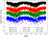 |
Fig. 2 Phase-folded light curve of B, V, R, I band photometry (bottom to top). Colours are as indicated in the legend. Additionally, we show the HOYS U band data in magenta. For clearer display of the brightness maximum we repeat the data and add 1.5 mag in each band except the I band. In the V band we mark with black diamonds the HOYS data taken at the time of the PENELLOPE observations, while the purple square represents HOYS photometry taken near the X-Shooter no. 2 observation. |
3.4 Flux calibration of UVES spectra
The UVES spectra are not absolutely flux calibrated, so we performed our own calibration using contemporaneous photometry. We calibrated the UVES flux using relative B and V band photometry to Vega with the photometric magnitudes of Vega, taken from Ducati (2002). We used an absolute flux calibrated spectrum of Vega taken by HST/STIS2 (Bohlin et al. 2014). The photometric coverage of V505 Ori quasi-simultaneous to the UVES and X-Shooter spectra is good. While there is at least one HOYS and AAVSO measurement closer than about one hour in the V band for all PENELLOPE spectra, in the HOYS data some B band measurements are missing. Since in B and V filter there is a very good agreement between HOYS and AAVSO, we used the AAVSO data generally. Only for the second X-Shooter spectrum taken in February 2020 the photometric measurements are taken about 5 hours before the spectrum and the AAVSO B band is missing. Therefore, we used the HOYS measurement instead. We then integrated the Vega spectrum over the two filters respectively using transmission curves for Johnson B and V filter to gain Fvega. The correction factors can be calculated by
![$\[corr=\frac{F_{{vega}}}{h \cdot c} \cdot 10^{\left(\left({mag }_{{star}}-{mag}_{{vega}}\right) /-2.5\right)},\]$](/articles/aa/full_html/2025/12/aa56230-25/aa56230-25-eq2.png) (1)
(1)
where h is the Planck constant and c is the speed of light. We scaled linearly between the correction factor for the B and V band for applying the actual wavelength dependent correction to the UVES spectra. We also checked the two X-Shooter spectra by doing the same calculations and got correction factors near to one. This is expected as the X-Shooter observations were already flux calibrated and validate our usage of Eq. (1) for the UVES spectra. We show all spectra in Fig. B.1.
4 Determination of veiling
Manara et al. (2021) list veiling measurements for the PENELLOPE spectra of V505 Ori (see Table 1). However, there have been no veiling measurements reported for the X-Shooter spectrum no. 2. Moreover, for our reddening analysis, we want to use the whole wavelength range of the UVES spectra and therefore need some additional veiling measurements at the very blue and red ends of the spectra. Since we follow a different method and want to have a denser wavelength sampling of veiling measurements, we redo the analysis also for the PENELLOPE spectra. A description of our used templates and models can be found in Sect. 3.3.
We followed the ansatz of Hartigan et al. (1989) that the observed spectrum is the sum of the photospheric flux Fphot,λ and the veiling flux Facc,λ caused by accretion. Veiling may consist of a continuum and emission lines, with the latter not considered here. To compute the veiling, we added excess flux, Facc,λ, (assumed to be constant in small wavelength intervals and causing the veiling of the photosphere) to a template spectrum (representing the photosphere of the star, Fphot,λ). The relative veiling was then defined as rλ = Facc,λ/Fphot,λ.
Since the archival HARPS template spectrum lacks errors we cannot use the analytic equation given by Hartigan et al. (1989) for computing the best-fitting constant but instead compute a χ2 best fit. We do this in 54 wavelength intervals between 4310 Å and 6750 Å. While the red end is determined by the wavelength coverage of the UVES spectra, the blue end is determined by the increasingly lower signal to noise (S/N) towards bluer wavelengths. Each interval has a typical length between 10 Å and 20 Å. The actual length is determined by gaps in the observed and template spectra, and by our omission of regions around emission lines or strong line blends. Emission lines encompass accretion sensitive lines, chromospheric lines, forbidden wind lines, and possibly an emission line veiling component. The latter was described by Rei et al. (2018); Armeni et al. (2024), and we show an example in Fig. 3 for an Fe I line at 5227.19 Å, which corresponds to the strong absorption line in the PHOENIX spectrum and is blue-shifted by 8–9 km s−1.
Generally, the veiling, rλ, determined with the HARPS template HD 200779, the weak-line TTauri star SO 879 (which we applied to the two X-Shooter spectra), and the PHOENIX model spectrum agree well with each other being all lower at longer wavelengths. This is compatible with accretion causing a hot (~10 000 K) spot on the stellar surface. In addition, rλ is lower for spectra taken at a lower brightness. Since there is some scatter in the measurements we computed mean veiling values in 150–200 Å wide wavelength intervals as shown in Fig. 4 and calculated the standard deviation. The values derived for the HARPS template and the PHOENIX model agree within 1σ except for the wavelength region from 4800 to 5500 Å, where they are in agreement within 2σ, with the PHOENIX values being systematically higher. We find also good agreement with the values determined by Manara et al. (2021) within 2σ as shown in Fig. 4 and in Table 1. The deviation between the methods is generally less than 5%, with our values usually being slightly smaller than the ones by Manara et al. (2021). The largest deviations occur for the r600 band and are about 20%. This comparison shows that our much simpler approach leads to comparable results than a more sophisticated analysis like the one in Manara et al. (2021). For the two X-Shooter spectra we also extended our measurements to higher wavelengths (7000 to 8500 Å) using the SO 879 template and found relative veiling values between 0.46 and 0.58 for the X-Shooter spectrum no. 1 and 0.45 and 0.73 for the X-Shooter spectrum no. 2, respectively. For even redder wavelengths we found no suitable lines, most probably since the spectrum of V505 Ori starts to get influenced by dust emission at these wavelengths, as can be seen in Fig. E.4 by Manara et al. (2021).
We are not interested in calculating mass accretion rates here since this has already been done by Manara et al. (2021). Nevertheless, we needed the veiling flux, Facc,λ, for the reddening measurements. For TW Hya Herczeg et al. (2023) found a constant veiling flux when the star was in a low-accretion state, while for some spectra taken during increased accretion, a higher veiling flux in the blue could be deduced. We found the veiling flux for each spectrum to be constant in wavelength within its standard deviation over the whole considered wavelength range, even for the UVES spectrum no. 1, where the median Facc,λ is the highest. In the reddening computation in the next section, we therefore used the median of the veiling flux for each spectrum.
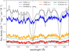 |
Fig. 3 Example of an emission line in the V505 Ori spectrum. The UVES spectra are shown in blue, orange, and red. The two X-Shooter spectra are in black and cyan. The grey spectrum is the PHOENIX spectrum normalised to the first UVES spectrum. The black dashed spectrum is the PHOENIX spectrum with veiling for the UVES spectrum no. 1 added (and again normalised). |
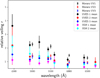 |
Fig. 4 Relative veiling. The relative veiling is shown for the wavelength range of the UVES spectra determined with the HARPS template star HD 200779. Shown are the mean values of corresponding 150–200 Å chunks in wavelength as dots with the colours indicating the different spectra as given in the legend. The crosses mark the relative veiling as found by Manara et al. (2021). |
5 Determination of extinction
We computed the extinction for each spectrum using the continuum fluxes from the wavelength intervals used for the veiling determination. We reddened the continuum fluxes of the template star HD 200779 after adding the median veiling flux. We used the unred function from the python PyAstronomy package (Czesla et al. 2019), which can be used to unredden or redden a spectrum. It uses the parametrisation of the normalised extinction curve by Fitzpatrick & Massa (1990) and allows the colour excess E(B-V) to be specified, which is related to the density of the interfering material and RV, which is a measure of the size of the grains the interfering material consists of. Then the total extinction AV = E(B − V) · RV can be calculated. We used here a grid of extinction values ranging in total extinction AV from 0.0 to 1.95 mag in steps of 0.05 mag and in RV from 1.6 to 9.1 in steps of 0.5. We calculated the best-fitting AV and RV combination by a reduced χ2 fit of the veiled and reddened template spectrum to our observed spectra of V505 Ori. We estimated standard deviations for our AV values by ![$\[1 \sigma=A_{V}\left(\chi_{{min }}^{2}+1\right)\]$](/articles/aa/full_html/2025/12/aa56230-25/aa56230-25-eq3.png) .
.
Applying this procedure, we find that for all our spectra within the 95% confidence level all RV values are possible. Also there is a degeneracy between AV and RV, implying larger AV values for larger RV values. This degeneracy has already been noticed by McJunkin et al. (2016) and Fuhrmeister et al. (2024). We show exemplarily our fitting results for UVES spectrum no. 2 in Fig. 5 (top panel). For the interstellar medium a canonical RV of 3.1 is typically used. Fixing RV to a value of 3.1 we find strongly varying extinction values for our different spectra ranging from AV=0.05 to 0.85 mag. We state the extinction values and their errors for each spectrum in Table 1. As cross-check we again used the SO 879 X-Shooter spectrum as template extending the AV measurements for the two X-Shooter spectra to 8500 Å and found values in agreement within 1σ with our fits with HD 200779 as template. Again we could not determine RV.
We show a comparison between veiled and reddened template continuum fluxes and the observed ones in Fig. 5 (bottom panel) for the first UVES spectrum; for the other spectra we show the same comparison in Figs. A.1 and A.2. We also checked that no satisfying fit can be established, if the veiling flux is not added to the template, with the deviation being worst for the UVES spectrum no. 1. We show this for the UVES no. 2 spectrum (second worst case) and the X-Shooter no. 1 spectrum (best case) in Fig. A.1.
The reference star HD 200779 has Teff=4400 K, like the applied PHOENIX spectrum. However, Manara et al. (2021) reported for the X-Shooter no. 1 spectrum Teff=4000 K and this value was also found from photometry (Manzo-Martínez et al. 2020). Therefore, we performed the above procedure also with a PHOENIX model for Teff=4000 K. This leads to higher veiling and higher extinction values in conjunction to acceptable but worse fits than for the higher photospheric temperature template even for the X-Shooter no. 1 spectrum, where the lower temperature was inferred from. We state the derived AV values in Table 1.
Regardless of the chosen template and setting, we find the lowest extinction for the UVES spectrum no. 1 at the optical brightness maximum and in conjunction with the highest veiling. Then with decreasing brightness, the veiling also decreases, while the extinction increases. Our extinction values can explain the spread of AV found in the literature. Although the systematic behaviour of AV is quite evident, the values of RV cannot be determined. Therefore, we cannot make any statements regarding the grain size of the intervening material.
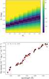 |
Fig. 5 Top: best-fitting AV and RV values for UVES spectrum no. 2. The black dot marks the best-fitting values, and the black, red, and blue contours mark the 68%, 90%, and 95% confidence level. Bottom: comparison of continuum flux density of V505 Ori (black dots) with the veiled and then reddened template (HD 200779) continuum fluxes (red asterisks) for the UVES no. 1 spectrum. |
6 Results from the photometry including TESS data
Froebrich et al. (2022) determined a photometric period and found that the phase-folded data show a slight asymmetry with a gradual, slow decay to the brightness minimum and a faster rise to the maximum. With more data, this systematic behaviour is less clearly seen, but the spread in the data especially around brightness minimum is even more evident as can be seen in Figs. 2 and 6. Looking at single cycles with a good phase coverage reveals amplitudes in V as low as about 0.6 mag and larger than 2 mag, with most amplitudes being about 1 to 1.5 mag. We state the mean amplitude for each filter for all HOYS data in Table 2. The error is dominated by the larger scatter around the minimum, which is about 0.5 mag for all filters, while the scatter for the maximum is 0.27–0.38 mag. The PENELLOPE data were taken during a period with a rather large amplitude (see Fig. 6). Even adjacent cycles can show very different depths and shapes (e.g. green diamonds and yellow asterisks in Fig. 6 with the latter showing an amplitude of more than one magnitude larger than the former). If dark spots caused this variability, they would have to show vigorous evolution on a timescale of a week to produce such a light curve.
Since the AAVSO and HOYS data with typically one data point per night are relatively coarsely sampled, we also had a look at the TESS data of sectors 6 and 32, which cover three to four rotation periods. We show the light curves in Fig. 7. While the periodic variability dominates the light curves, more substructure than in the ground-based photometry can be identified. For example, rise and decay seem to be relatively symmetric. Moreover, the brightness maximum is quite spiky several times, which would not be expected for a typical quasi-periodic dipper (see Fig. 9 in, Cody et al. 2014). On the other hand, at least sometimes there is more substructure in the minima than judged from the ground-based photometry (see Figs. 1 and 6). Especially interesting is the recurrent feature in sector 6 at about days 7 and 14, which could be caused by an additional absorbing structure. However, this structure shows some evolution during one revolution and vanished by the time of sector 32. Such behaviour would be quite typical for a quasi-periodic dipper. We therefore calculated the Q-M-metric defined by Cody et al. 2014; Cody & Hillenbrand 2018 and obtain M=0.05 and −0.06 and Q=0.21 and 0.16 for the TESS sectors 6 and 32, respectively. This places V505 Ori in the quasi-periodic symmetric category at the threshold to periodic symmetric. Computing the metric for the V band AAVSO data leads to M=0.02 and Q=0.45 also in the quasi-periodic symmetric regime. Moreover, the very spiky peaks in some cycles can be interpreted as either bursts recurrent at maximum brightness or as an indication that the star is (almost) never seen fully.
Furthermore, we computed a Lomb-Scargle periodogram (Lomb 1976; Scargle 1982) for each sector and found a period of 7.3 ± 1.1 days for sector 6 and a period of 6.94 ± 0.73 days for sector 32 with a false-alarm probability of less than 10−5 in both cases. The inferred periods are in agreement with the ones from the HOYS and AAVSO data of 7.0814 ± 0.0004 days, which is very stable over our long time baseline of more than five years, allowing for the much higher precision than the TESS data with only a few periods covered.
We also revisited the colour diagrams of Froebrich et al. (2022), but with different colours in Fig. 8. We show the measurements taken at the time of the PENELLOPE observations as black symbols. These individual measurements follow about the slope of the full dataset. From the indicated extinction vectors, it can be seen that extinction should play a role, but cannot explain the full variations we see, a conclusion also drawn by Froebrich et al. (2022).
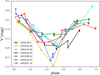 |
Fig. 6 V band magnitude of selected cycle epochs. This is illustrating the spread in depth and shape of the individual dimming events in V505 Ori. While the green diamonds mark an especially shallow cycle, the yellow asterisks and blue triangles mark deep cycles. |
Measured photometric amplitudes (input for the spot models).
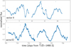 |
Fig. 7 Normalised TESS light curves of V505 Ori in sector 6 and 32. Next to the dominating periodic structure, more details of variability can be seen. For example, in sector 6 there is the additional dip at about day 7, which re-occurs at about day 14. |
7 Emission lines
There are many emission lines present in the spectrum of V505 Ori. First, there are some forbidden lines, which are associated with stellar or disk winds and have been discussed already by Gangi et al. (2023) and Maucó et al. (2025). Other emission lines are typically associated with the accretion flow – although chromospheric activity may contribute to their flux (Stelzer et al. 2013). Exemplarily, we present the profiles of Ca II K, Hβ, Mg I at 5167 Å, Fe II at 5317 Å, Na I D at 5889.95 Å, and He I D3 at 5875.62 Å in Fig. 9. Additionally, we show the Hα line, the Na I D at 5895.92 Å, and the Ca II H lines in Fig. B.3. There are several accretion features found in the different lines. We analysed, first, broad emission lines and, second, lines with a (transient) narrow and broad component (NC, BC).
Regarding the broad emission lines, we concentrated on the hydrogen lines, the Ca II H and K lines, and the Na I D lines. Exemplarily for the broad lines we measured de-reddened Hα line fluxes, which decrease for the three UVES and the X-Shooter spectrum no.1, while the equivalent width (EW) shows the opposite trend, which is purely a continuum effect. Both, EW and flux measurements can be found in Table 1. The same trends are seen for Hβ. We calculated mass accretion rates from our Hα line flux measurements using the correlation with Lacc, stellar radius (R = 1.56RSun), and truncation radius (Rin = 2.78R) given by Pittman et al. (2025a) and we find values log10 ![$\[\dot{M}_{\text {acc}}\]$](/articles/aa/full_html/2025/12/aa56230-25/aa56230-25-eq8.png) = −8.3 to −8.55 (in M⊙/yr) for brightness maximum to minimum. Given the uncertainty in the relation between Lacc and LHα the measured range in log10
= −8.3 to −8.55 (in M⊙/yr) for brightness maximum to minimum. Given the uncertainty in the relation between Lacc and LHα the measured range in log10 ![$\[\dot{M}_{\text {acc}}\]$](/articles/aa/full_html/2025/12/aa56230-25/aa56230-25-eq9.png) is consistent with no variability. It is also in agreement with values found in the literature for V505 Ori ranging from −7.7 to −8.54 (Pittman et al. 2025a; Maucó et al. 2016).
is consistent with no variability. It is also in agreement with values found in the literature for V505 Ori ranging from −7.7 to −8.54 (Pittman et al. 2025a; Maucó et al. 2016).
The Na I D lines show a very complicated line profile, since emission is found on top a strong photospheric absorption line. To disentangle the different line components, we subtracted from each spectrum the best-fitting model from Sect. 8.2, which accounts for the photospheric, veiling, reddening contribution, and grey extinction. We show the subtracted line in Fig. B.3. The residual broad emission line must be originating from the accretion process (and possibly winds).
In all these broad lines present in the UVES no. 1 spectrum (and in the X-Shooter no. 2 spectrum) a broad absorption feature is present in the red wings of these broad emission lines. This is best seen in Fig. 9 for Hβ at about 200 km s−1 but can be identified also in other Balmer lines, the Ca II H and K, and the Na I D lines at velocities of 180–220 km s−1 for the deepest absorption. For the Na I D lines this is best seen in the subtracted spectra in Fig. B.3 in the Na I D1 line. For the Ca II K line the feature is weak, indicating, that the much stronger absorption red-wards of the Ca II H line is caused by Hϵ (cf., Figs. 9 and B.3). In the red part of the X-Shooter no. 2 spectrum the same feature is also found in the Paschen, the Bracket, and the He I infrared triplet (IRT) lines. There we found the velocity varying between 180 (Br 7; very weak absorption) and 320 km s−1 (Ca II K). Since the He I IRT lines have strong diagnostic potential (Fischer et al. 2008), we show them in Fig. B.3. While in the X-Shooter no. 2 spectrum a pronounced red absorption is noted, the same feature is much weaker in the X-Shooter no. 1 spectrum. Generally, such features have been interpreted as a sign of magnetospheric infall (Muzerolle et al. 2001; Hartmann et al. 2016).
Next, we analysed emission line profiles, which show a NC and BC. Helium NC lines of slight redshift have been interpreted to be formed in the post-shock region by Beristain et al. (2001); Pouilly et al. (2021). The NC of the metal lines is instead thought to be formed in the heated photosphere below the shock, where the gas has been already decelerated to merge with the photosphere. Finally, the BC is thought to be formed in the accretion flow itself, with higher excitation lines formed near the accretion shock (Sicilia-Aguilar et al. 2015; Armeni et al. 2024).
We detected He I lines at 5875 and 6678 Å, which both display only a NC and are slightly redshifted (<10 km s−1). They are detected with similar EW in each spectrum as can be seen in the continuum-normalised spectra in Fig. 9. Nevertheless, since the continuum is going down to brightness minimum, the helium line flux is as well (like the Hα line flux). This suggests that we see the accretion spot all the time to some extent.
We show examples of metal lines with a NC and BC again in Fig. 9: The Fe II line at 5316.61 Å and the Mg I triplet line at 5167.32 Å, which is blended in the broad component with an Fe II line at 5169.03 Å. While the BC are prominently present only in the UVES no. 1 spectrum, the NC may be present in all spectra, although it is much weaker towards brightness minimum. This suggests, that we see the accretion stream mainly in the UVES spectrum no. 1, while the photospheric region below the accretion spot is also at least partly present in the other UVES spectra. The difference to the NC of the Helium lines can be explained by the heated part of the photosphere covering a larger area than the post-shock region. The BCs have blueshifts of about −30 km s−1, but with large errors since they are very broad, noisy, and often blended. The NC of the metal lines in the UVES spectrum no. 1 is typically slightly blue-shifted from ~0 to −8 km s−1 and in many cases in agreement with photospheric velocity as expected.
We conclude that different spectral indicators suggest that we are observing the accretion funnel most directly in the line of sight at maximum brightness of V505 Ori, while there are fewer accretion imprints in the other spectra (as evidenced for example by the BC of several lines or the broad red absorption feature in the Balmer lines). Also, the accretion spot and the region below show its presence most prominently in the UVES spectrum no. 1 as indicated by the NC but it must be seen to some extent all the time, since helium emission is observed in all spectra.
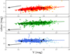 |
Fig. 8 Colour diagram with respect to V band photometry. Red (HOYS) and orange (AAVSO) dots represent V-I, green (HOYS) and light green (AAVSO) dots represent V-R, and blue (HOYS) and light blue (AAVSO) dots represent B-V. The solid coloured lines represent the best linear fit to the data, while the black arrows represent the extinction correction for AV=1.0 mag and RV=3.1. The black symbols denote the mean measurements during the days of the PENELLOPE observations. |
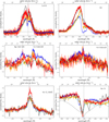 |
Fig. 9 Examples of emission lines in V505 Ori. The UVES no. 1 spectrum is shown in blue, no. 2 in orange, no. 3 in red, X-Shooter spectrum no. 1 in black, and X-Shooter no. 2 in cyan. As a dashed vertical line, we show the central wavelength of the respective line. Top left: Ca II K line. Top right: Hβ line. Middle left: Mg I line at 5167.32 Å. Middle right: Fe II line at 5316.61 Å. Bottom left: He I D3 line. Bottom right: blue Na I D line at 5889.95 Å. In grey we plot a PHOENIX photospheric spectrum with Teff=4400 K. |
8 Discussion
Possible explanations for the periodic variations in the photometric data of V505 Ori are spots on the stellar surface or an AA Tau-like warped inner wall of the accretion disk (Bouvier et al. 1999; McGinnis et al. 2015). Such disk deformations in conjunction with accretion processes are expected from (two and three dimensional) magneto-hydrodynamic simulations if the rotation axis is misaligned to the axis of the poloidal magnetic field (Romanova et al. 2013; Romanova & Owocki 2015). Froebrich et al. (2022) could not identify a reasonably fitting spot model and therefore decided for a warped disk, although they found that the slopes determined from their colour-magnitude plots could not be explained by invoking only extinction. In our spectral analysis we found additionally, that the highest extinction is seen at the dimmest state, when the veiling is lowest. This is in contrast to the scenario for AA Tau-like stars, where the hot accretion spot occurs together with the extinction event by the disk wall, since both are coupled to the accretion flow.
8.1 Spot model fitting
We therefore revisited the spot model scenario from Froebrich et al. (2022) in the light of the information gained from the spectroscopy. They applied a spot model to their mean amplitudes in the different photometric bands. Since the amplitudes of the different epochs can differ quite considerably, we look at the individual epochs for the PENELLOPE observations to apply our extinction values. Moreover, we also take into account spots, which are circumpolar and therefore can be seen to some extent all the time. We alter Eq. (1) from Froebrich et al. (2022) in the following way:
![$\[A_\lambda^{{model }}=-2.5 \times \log \left(\frac{\left(1-f_{min }\right) \times F_{\lambda ~{ extinct }}^*+f_{min } \times F_{\lambda ~{ extinct }}^{{spot }}}{(1-f) \times F_{\lambda ~{ extinct }}^*+f \times F_{\lambda ~{ extinct }}^{{spot }}}\right).\]$](/articles/aa/full_html/2025/12/aa56230-25/aa56230-25-eq10.png) (2)
(2)
Here, ![$\[A_{\lambda}^{model}\]$](/articles/aa/full_html/2025/12/aa56230-25/aa56230-25-eq11.png) is the amplitude of the spot model in a certain photometric band,
is the amplitude of the spot model in a certain photometric band, ![$\[F_{\lambda}^{*}\]$](/articles/aa/full_html/2025/12/aa56230-25/aa56230-25-eq12.png) and
and ![$\[F_{\lambda}^{{spot}}\]$](/articles/aa/full_html/2025/12/aa56230-25/aa56230-25-eq13.png) are the stellar photospheric flux and the flux from the spot in the corresponding photometric filter, respectively. Since during minimum brightness we found a significant reddening of the spectra, we apply this here to the minimum flux of both the spot and the star,
are the stellar photospheric flux and the flux from the spot in the corresponding photometric filter, respectively. Since during minimum brightness we found a significant reddening of the spectra, we apply this here to the minimum flux of both the spot and the star, ![$\[F_{\lambda ~{extinct}}^{{spot}}, F_{\lambda ~{extinct}}^{*}. f\]$](/articles/aa/full_html/2025/12/aa56230-25/aa56230-25-eq14.png) is the maximal spot covering fraction and fmin is the minimum spot covering fraction, when most of the spot is rotated behind the star. We computed the best-fitting model using a χ2 minimisation, for all differential photometry including the time of either the UVES no. 1 spectrum or the X-Shooter no. 1 spectrum. To compute the amplitudes, we used mean values from the days of the spectral observations in each HOYS filter and list them in Table 2. Since the errors are comparable for the different days in the different filters, we use typical errors for each filter, also listed in Table 2. Since the differences between the UVES no. 3 spectrum and the X-Shooter no. 1 spectrum is smaller than the errors, and there is a deviating behaviour in the U band for this time, we omit the UVES no. 3 spectrum from the calculations. There is only a B band HOYS measurement for the maximum brightness state, and therefore we used AAVSO measurements for the other times as the agreement of HOYS and AAVSO in the B band is compatible with the typical spread of about 0.1 to 0.15 mag.
is the maximal spot covering fraction and fmin is the minimum spot covering fraction, when most of the spot is rotated behind the star. We computed the best-fitting model using a χ2 minimisation, for all differential photometry including the time of either the UVES no. 1 spectrum or the X-Shooter no. 1 spectrum. To compute the amplitudes, we used mean values from the days of the spectral observations in each HOYS filter and list them in Table 2. Since the errors are comparable for the different days in the different filters, we use typical errors for each filter, also listed in Table 2. Since the differences between the UVES no. 3 spectrum and the X-Shooter no. 1 spectrum is smaller than the errors, and there is a deviating behaviour in the U band for this time, we omit the UVES no. 3 spectrum from the calculations. There is only a B band HOYS measurement for the maximum brightness state, and therefore we used AAVSO measurements for the other times as the agreement of HOYS and AAVSO in the B band is compatible with the typical spread of about 0.1 to 0.15 mag.
To calculate the model amplitude, ![$\[A_{\lambda}^{model}\]$](/articles/aa/full_html/2025/12/aa56230-25/aa56230-25-eq15.png) , we used PHOENIX (Hauschildt et al. 1999) model spectra from the latest library (Husser et al. 2013). For the stellar photosphere, we used a model with Teff=4400 K, log g=4.5, and solar chemical composition. For the spot we used a model grid of Teff=3600, 3800, 4000, 4100, 5000, 5500, 6000, 6500, 7000, 7500, 8000, 9000, 10 000, 11 000, and 12 000 K. If applicable, as deduced from the spectral fitting, we applied the reddening to the PHOENIX spectra by using again the unred function as described in Sect. 5. We performed our best-fit search on a grid of f=0.001 to 0.496 in steps of 0.005, and for fmin=0.001 to 0.277 this was done in steps of 0.004.
, we used PHOENIX (Hauschildt et al. 1999) model spectra from the latest library (Husser et al. 2013). For the stellar photosphere, we used a model with Teff=4400 K, log g=4.5, and solar chemical composition. For the spot we used a model grid of Teff=3600, 3800, 4000, 4100, 5000, 5500, 6000, 6500, 7000, 7500, 8000, 9000, 10 000, 11 000, and 12 000 K. If applicable, as deduced from the spectral fitting, we applied the reddening to the PHOENIX spectra by using again the unred function as described in Sect. 5. We performed our best-fit search on a grid of f=0.001 to 0.496 in steps of 0.005, and for fmin=0.001 to 0.277 this was done in steps of 0.004.
We found that models with spot temperature below the photospheric temperature are incompatible with the data at 95% confidence level (deduced from the best-fitting temperature and filling factors) for all combinations of filling factors and all photometric amplitudes. Therefore, we exclude a cold spot as reason for the brightness variations.
For hot spots on the other hand, there is some degeneracy between spot temperature and filling factor. In particular, spot temperatures below 6500 K lead to a filling factor greater than 20–30%. Therefore, we fix the spot temperature to 9000 K, which we consider a realistic average value for the post-accretion shock temperature. For the spot temperature of 9000 K the filling factors for the different dates derived from the different amplitudes are in agreement with each other. We show this in Fig. 10. There the filling factor at the date of the UVES spectrum no. 2 is the minimum filling factor in the middle panel and the maximum filling factor in the lower panel. Intercomparison of the best-fitting models of the different amplitudes leads to estimates of the bright spot filling factors of 18–21% for the data taken simultaneously to UVES spectrum no. 1, of 10% for UVES spectrum no. 2, and of 3–4% for the X-Shooter no. 1 spectrum at brightness minimum. We conclude, therefore, that the brightness variations can be explained by a circumpolar spot, which has an extension of about 20% when it is fully seen and only about 5% at brightness minimum when the viewing angle allows only part of it to be seen.
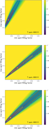 |
Fig. 10 Best-fitting max and min filling factor of the star spot model for the spot temperature set to 9000 K. The orange dots mark the best-fitting model, and the orange, red, and blue contour lines mark the 68%, 90%, and 95% confidence levels. Colours indicate χ2 as shown by the colour bar. Top: amplitude calculated for photometry taken at the date of UVES spectrum no. 1 and X-Shooter spectrum no. 1. Middle: amplitude calculated for the photometry taken at the date of UVES spectrum no. 1 and 2. Bottom: amplitude calculated for the photometry taken at the date of UVES spectrum no. 2 and X-Shooter spectrum no. 1. Intercomparison of the different panels lead to a spot filling factor for the date of UVES spectrum no. 1 of 18–21%, for no. 2 of 10%, and for the date of the X-Shooter spectrum no. 1 of 3–4%. |
8.2 Spectral fitting
We wanted to complement the modelling of the photometry with modelling of the observed spectra. We followed Schneider et al. (2018, see also Frasca et al. 2020), who modelled the spectra of V354 Mon with different fractions of the light (i) coming from the unperturbed stellar surface; (ii) passing through the outer disk layers, and therefore being reddened; and (iii) being blocked from view by dense layers of the disk. Since we observed V505 Ori nearly edge-on, we regard parts of the stellar disk being totally obscured by the disk as probable. In our model we account for (i) light from the hot accretion spot Facc, (ii) light from the stellar surface Ftheo, and (iii) light being completely extinct F0, with (i) and (ii) being reddened. Since our template spectrum has no absolute flux calibration, we again used the PHOENIX model spectra with Teff=4400 and 4000 K as templates with radius R = 1.56 R⊙ (Pittman et al. 2025a) and distance d = 392 ± 4 pc (Manara et al. 2021) for the calculation of the flux at Earth, Ftheo · Our model flux, Fmodel, was calculated as follows:
![$\[F_{\mathrm{model}}=\left(F_{\mathrm{acc}} \times f_1+F_{\mathrm{theo}} \times f_2\right) \times { reddening }+F_0 \times f_3,\]$](/articles/aa/full_html/2025/12/aa56230-25/aa56230-25-eq16.png) (3)
(3)
with the filling factors f1 + f2 + f3 = 1. We neglect in our model a possible part of the star from which the light is not reddened, since the agreement between observed spectra and veiled and reddened template spectra in Sect. 5 is quite good. As reddening we apply here the individual AV s with RV = 3.1 from Sect. 5 for each spectrum. Alternatively, we tried to model the spectra with negligible reddening of AV=0.05 mag applied.
Since the PHOENIX spectra lack, for example, emission lines, the general agreement is only moderate, leading to non-unique solutions. Since most of the models led to a veiling flux of 1015 erg s−1 cm−2 cm−1, we fixed this for the rest of the model calculations. With reddening from Sect. 5 applied, this led to filling factors of the hot spot f1 going down from 10% filling (UVES spectrum no. 1) to 5% filling (X-Shooter spectrum no. 1) for both Teff=4400 and 4000 K. The filling factor of reddened light f2 is higher for Teff = 4000 K going down from 50% to 30%, while for Teff=4400 K it ranges from 25% down to 15% and accordingly for f3 (blocked light) going up from 65% to 80% Teff=4400 K, and from 40% to 65% for Teff=4000 K. Fixing the reddening to AV=0.05 mag led to slightly smaller accretion spots (down to 1%) and to slightly to moderately worse fits for both effective temperatures.
From a physical point of view, the spectral model is even more sophisticated than the spot model, since it additionally includes a totally obscured part of the stellar surface. This is possible since there is additional information about the absolute fluxes in the spectra. This allows us to infer that a significant part of the stellar surface is totally blocked from view by the disk. For very high inclinations like in V505 Ori this may be expected, especially since there are only small variations in the obscured part f3 from spectrum to spectrum. Although this information cannot be deduced from the spot model, the spot model may be more robust, since the agreement between PHOENIX model spectra and observed spectra is in detail only moderate. A comparison of the spectral modelling and the photometric spot model in Sect. 8.1 shows that for the spectral model including reddening there is rough agreement about the size of the accretion spot at the different times.
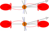 |
Fig. 11 Scenario for V505 Ori. The vertical black line marks the rotation axis, while the inclined black line marks the viewing horizon on the stellar disk. The dashed blue line marks the magnetic axis. The red lines represent the accretion funnels hitting the star near to the magnetic axis and creating the hot accretion spot there. The (opaque) disk is shown in red here and the dotted black line marks the part of the star, which is blocked from view by the disk. The (asymmetric) pink areas mark less dense parts of the disk, which lead only to reddening of the passing light. Top: brightness maximum. Here, the accretion spot can be fully seen, leading to the highest veiling and some imprint of the accretion funnel in the spectrum. Bottom: brightness minimum. Here, only a small part of the accretion spot can be seen, and the accretion funnel cannot be viewed. |
8.3 Scenario
We present our scenario for V505 Ori in Fig. 11. The system is seen nearly edge-on. We find in Sect. 8.2 that a large part of the stellar surface is totally obscured all the time (f3 = 40–80%). This implies very high inclinations in agreement with i = 80° from Gangi et al. (2023). Furthermore, we estimate the inclination by using sin i = v sin i · Prot/2πR). With the stellar radius R = 1.56 R⊙ (Pittman et al. 2025a), v sin i = 13km s−1 (Manara et al. 2021), and Prot = 7 days we calculate sin i = 1.16, which suggests also very high inclination. The non-physical value of 1.16 may be caused by (i) a too high v sin i value (where comparison by eye to our PHOENIX model shows that values as low as 11 km/s lead to acceptable fits), (ii) a wrong radius estimate (whose calculation did not take into account, that part of the star is occulted), or (iii) the true rotation period of the star being lower than the observed period.
Moreover, we deduced a hot spot at high latitudes from our photometric light curve modelling in Sect. 8.1 and the spectral analysis in Sect. 8.2. We propose a rather small angle Θ between the magnetic axis and the rotation axis comparable to the complementary angle of the inclination. This ensures that the accretion spot is seen for any rotational phase of the star but with different filling factors (cf., Fig. 11). On the other hand, the angle must not be too small, since the models by Kulkarni & Romanova (2013) suggest, that Θ < 5° leads to closed ring shaped accretion spots. In this case, we would see about the same filling factor for the spot all the time. Therefore, Θ should be about 10° to 20°.
When the hot spot is pointing to the observer and has therefore its largest filling factor also the accretion funnel is directly seen as evidenced in the spectra by the veiling and the spectral line features (see Sect. 7). When the hot spot is only partly seen and therefore has smaller filling factors, the accretion funnel is not observed directly; instead the line of sight passes through some disk material causing reddening and additional obscuration of the stellar disk. If this additional obscuration is caused by a disk warp opposite the accretion spot, it should be located at the co-rotation radius rc = (P/2π)2/3(GM*)1/3 = 9.2 R* with M* = 0.81 M⊙ taken from Pittman et al. (2025a). This leads to an irradiation temperature T ~ 1300 K using the stellar luminosity L* = 0.56L⊙ at the distance rc, which would allow for the formation of dust grains.
We also found some variability in the system. The different depth of the minima in the photometric light curve suggests variability in the strength of the accretion flow or a variable size of the accretion spot. Moreover, also the extent or location of the accretion funnel may vary: The X-Shooter no. 2 spectrum (taken 10 month earlier than the other spectra) suggests at least some variability there, since also some imprints of the accretion funnel are seen in the spectrum at a phase comparable to the UVES no. 2 spectrum which does not show signs of the funnel. Nevertheless, the AV and also the veiling of the two spectra are comparable.
Some unsettled questions remain. It is puzzling that the highest reddening is observed during brightness minimum, while usually magnetohydrodynamic (MHD) models predict that the highest reddening is seen together with the accretion spot (Romanova & Owocki 2015) as the spot is in phase with the (base of the) accretion funnel. The additional reddening may also be caused by disk or stellar winds crossing the line of sight (Johns & Basri 1995), which is a possibility, since the star exhibits strong forbidden wind lines (Gangi et al. 2023) and also shows variable blue shifted Hα absorption. This would also explain the strong variability of the minima in the photometric light curve if the wind is variable. However, Pittman et al. (2025b) found the star to be in the unstable ordered accretion regime. This is an argument in favour of disk occultation causing the (main) part of the variation, since it is hard to explain how the period can be so stable over years if it is caused mainly by unstable accretion.
9 Conclusions
We have analysed three UVESs and two X-Shooter spectra of the CTTS V505 Ori, where the UVES spectra and one X-Shooter spectrum were taken on consecutive days covering one brightness decrease from maximum to minimum. This periodic brightness variation had already been discovered in photometric data with a period of 7 days (Froebrich et al. 2022) and therefore the star was tentatively classified as AA Tau-like periodic dipper. From the brightness maximum to the minimum, we found decreasing veiling and increasing reddening of the spectra.
Revisiting of the spot model by Froebrich et al. (2022) using individual measurements in different filters at the respective times of the PENELLOPE spectra leads to a high-latitude accretion spot, whose filling factor varies between 5% and 20% of the visible hemisphere. From spectral modelling with PHOENIX model spectra, we found similar numbers for the area of the hot spot (but at maximum 10% filling) and that up to about 80% of the star is occulted by the disk during the brightness minimum. The variable filling factor of the hot (accretion) spot is in line with the decreasing veiling observed for the dimming spectra, while the higher occultation by the disk seems to explain at least part of the dimming, while another part originates in the smaller hot accretion spot. Additionally, we measured increasing reddening for lower brightness states. This indicates a warp opposite the accretion funnel, which is not totally opaque but reddens the observed spectra.
For the maximum brightness state, we found direct imprints of the accretion funnel in the spectrum, such as a broad and a narrow component in several strong emission lines and a red absorption component in higher Balmer lines and the Ca II H and K lines. This is in contrast to AA Tau-like objects, where the highest veiling is observed at the brightness minimum together with the accretion funnel imprints. The shape of the light curve does not suggest V505 Ori to be a periodic dipper since it lacks times of constant flux at the brightness maximum, and the minima are typically too regularly shaped. Nevertheless, it seems that the reddening variations are caused by a disk warp, which contributes by its extinction to the brightness variations. Also, the TESS photometric light curve, at least in sector 6, suggests additional absorbing structures at the co-rotation radius. The computation of the metric by Cody & Hillenbrand (2018) makes V505 Ori fall into their quasi-periodic symmetric category. Our analysis shows that the brightness variations can be explained by circumpolar rotation of the accretion spot but also that variable obscuration by the disk and dipper-like extinction (although with a different geometry than for AA Tau) play a role here. Therefore, V505 Ori exhibits signs of different variability classes.
The X-Shooter spectrum no. 2 taken 10 months earlier than the rest of the data indicates some long-term changes in the accretion properties since the accretion funnel is imprinted on the stellar spectrum unlike the UVES spectrum no. 2, which was taken at a very similar phase of the brightness cycle. The reason for the different depth of the individual brightness minima remains unclear and may be caused by either variations in the size or location of the accretion spot or by changes in the amount or location of the obscuring material. Observations covering another rotation cycle of V505 Ori are needed to gain some insights there. This makes V505 Ori an interesting object for a high-resolution spectral monitoring campaign.
Acknowledgements
The authors acknowledge funding through Deutsche Forschungsgemeinschaft DFG program IDs EI 409/20-1 and SCHN 1382/4-1 in the framework of the YTTHACA project (Young stars at Tübingen, Tautenburg, Hamburg & ESO – A Coordinated Analysis). For DFG: project code MA 8447/1-1. PCS acknowledges support by the DLR under grants 50 OR 50OR 2205 and 2412. Funded by the European Union (ERC, WANDA, 101039452). Views and opinions expressed are however those of the author(s) only and do not necessarily reflect those of the European Union or the European Research Council Executive Agency. Neither the European Union nor the granting authority can be held responsible for them. This work benefited from discussions with the PENELLOPE team and especially with R. Garcia Lopez. This work made use of PyAstronomy (Czesla et al. 2019), which can be downloaded at https://github.com/sczesla/PyAstronomy.
References
- Alencar, S. H. P., Teixeira, P. S., Guimarães, M. M., et al. 2010, A&A, 519, A88 [NASA ADS] [CrossRef] [EDP Sciences] [Google Scholar]
- Alencar, S. H. P., Bouvier, J., Donati, J. F., et al. 2018, A&A, 620, A195 [NASA ADS] [CrossRef] [EDP Sciences] [Google Scholar]
- Armeni, A., Stelzer, B., Frasca, A., et al. 2024, A&A, 690, A225 [NASA ADS] [CrossRef] [EDP Sciences] [Google Scholar]
- Beristain, G., Edwards, S., & Kwan, J. 2001, ApJ, 551, 1037 [Google Scholar]
- Bohlin, R. C., Gordon, K. D., & Tremblay, P. E. 2014, PASP, 126, 711 [NASA ADS] [Google Scholar]
- Bouvier, J., Chelli, A., Allain, S., et al. 1999, A&A, 349, 619 [NASA ADS] [Google Scholar]
- Bouvier, J., Alencar, S. H. P., Boutelier, T., et al. 2007, A&A, 463, 1017 [NASA ADS] [CrossRef] [EDP Sciences] [Google Scholar]
- Claes, R. A. B., Campbell-White, J., Manara, C. F., et al. 2024, A&A, 690, A122 [NASA ADS] [CrossRef] [EDP Sciences] [Google Scholar]
- Cody, A. M., & Hillenbrand, L. A. 2018, AJ, 156, 71 [Google Scholar]
- Cody, A. M., Tayar, J., Hillenbrand, L. A., Matthews, J. M., & Kallinger, T. 2013, AJ, 145, 79 [Google Scholar]
- Cody, A. M., Stauffer, J., Baglin, A., et al. 2014, AJ, 147, 82 [Google Scholar]
- Czesla, S., Schröter, S., Schneider, C. P., et al. 2019, PyA: Python astronomyrelated packages [Google Scholar]
- Ducati, J. R. 2002, VizieR Online Data Catalog: Catalogue of Stellar Photometry in Johnson’s 11-color system., CDS/ADC Collection of Electronic Catalogues, 2237, 0 (2002) [Google Scholar]
- Evitts, J. J., Froebrich, D., Scholz, A., et al. 2020, MNRAS, 493, 184 [Google Scholar]
- Feinstein, A. D., Montet, B. T., Ansdell, M., et al. 2020, AJ, 160, 219 [Google Scholar]
- Ferraz-Mello, S. 1981, AJ, 86, 619 [NASA ADS] [CrossRef] [Google Scholar]
- Fischer, W., Kwan, J., Edwards, S., & Hillenbrand, L. 2008, ApJ, 687, 1117 [Google Scholar]
- Fischer, W. J., Hillenbrand, L. A., Herczeg, G. J., et al. 2023, in Astronomical Society of the Pacific Conference Series, 534, Protostars and Planets VII, eds. S. Inutsuka, Y. Aikawa, T. Muto, K. Tomida, & M. Tamura, 355 [Google Scholar]
- Fischer, W. J., Battersby, C., Johnstone, D., et al. 2024, AJ, 167, 82 [NASA ADS] [CrossRef] [Google Scholar]
- Fitzpatrick, E. L., & Massa, D. 1990, ApJS, 72, 163 [NASA ADS] [CrossRef] [Google Scholar]
- Frasca, A., Manara, C. F., Alcalá, J. M., et al. 2020, A&A, 639, L8 [NASA ADS] [CrossRef] [EDP Sciences] [Google Scholar]
- Froebrich, D., Campbell-White, J., Scholz, A., et al. 2018, MNRAS, 478, 5091 [Google Scholar]
- Froebrich, D., Eislöffel, J., Stecklum, B., Herbert, C., & Hambsch, F.-J. 2022, MNRAS, 510, 2883 [Google Scholar]
- Fuhrmeister, B., Schneider, P. C., Sperling, T., et al. 2024, A&A, 692, A69 [NASA ADS] [CrossRef] [EDP Sciences] [Google Scholar]
- Gangi, M., Nisini, B., Manara, C. F., et al. 2023, A&A, 675, A153 [NASA ADS] [CrossRef] [EDP Sciences] [Google Scholar]
- Hartigan, P., Hartmann, L., Kenyon, S., Hewett, R., & Stauffer, J. 1989, ApJS, 70, 899 [NASA ADS] [CrossRef] [Google Scholar]
- Hartmann, L., Herczeg, G., & Calvet, N. 2016, ARA&A, 54, 135 [Google Scholar]
- Hauschildt, P. H., Allard, F., & Baron, E. 1999, ApJ, 512, 377 [Google Scholar]
- Herczeg, G. J., Chen, Y., Donati, J.-F., et al. 2023, ApJ, 956, 102 [NASA ADS] [CrossRef] [Google Scholar]
- Hernández, J., Calvet, N., Perez, A., et al. 2014, ApJ, 794, 36 [CrossRef] [Google Scholar]
- Husser, T.-O., Wende-von Berg, S., Dreizler, S., et al. 2013, A&A, 553, A6 [NASA ADS] [CrossRef] [EDP Sciences] [Google Scholar]
- Johns, C. M., & Basri, G. 1995, ApJ, 449, 341 [Google Scholar]
- Joy, A. H. 1945, ApJ, 102, 168 [Google Scholar]
- Kulkarni, A. K., & Romanova, M. M. 2013, MNRAS, 433, 3048 [NASA ADS] [CrossRef] [Google Scholar]
- Lomb, N. R. 1976, Ap&SS, 39, 447 [Google Scholar]
- Manara, C. F., Frasca, A., Venuti, L., et al. 2021, A&A, 650, A196 [NASA ADS] [CrossRef] [EDP Sciences] [Google Scholar]
- Manzo-Martínez, E., Calvet, N., Hernández, J., et al. 2020, ApJ, 893, 56 [CrossRef] [Google Scholar]
- Maucó, K., Hernández, J., Calvet, N., et al. 2016, ApJ, 829, 38 [CrossRef] [Google Scholar]
- Maucó, K., Briceño, C., Calvet, N., et al. 2018, ApJ, 859, 1 [CrossRef] [Google Scholar]
- Maucó, K., Manara, C. F., Ansdell, M., et al. 2023, A&A, 679, A82 [NASA ADS] [CrossRef] [EDP Sciences] [Google Scholar]
- Maucó, K., Manara, C. F., Bayo, A., et al. 2025, A&A, 693, A87 [NASA ADS] [CrossRef] [EDP Sciences] [Google Scholar]
- McGinnis, P. T., Alencar, S. H. P., Guimarães, M. M., et al. 2015, A&A, 577, A11 [NASA ADS] [CrossRef] [EDP Sciences] [Google Scholar]
- McJunkin, M., France, K., Schindhelm, R., et al. 2016, ApJ, 828, 69 [NASA ADS] [CrossRef] [Google Scholar]
- Muzerolle, J., Calvet, N., & Hartmann, L. 2001, ApJ, 550, 944 [Google Scholar]
- Oliveira, J. M., Jeffries, R. D., & van Loon, J. T. 2004, MNRAS, 347, 1327 [NASA ADS] [CrossRef] [Google Scholar]
- Percy, J. R., & Mattei, J. A. 1993, Ap&SS, 210, 137 [Google Scholar]
- Pittman, C. V., Espaillat, C. C., Robinson, C. E., et al. 2025a, ApJ, 992, 134 [Google Scholar]
- Pittman, C. V., Espaillat, C. C., Zhu, Z., et al. 2025b, ApJ, accepted [arXiv:2509.03767] [Google Scholar]
- Pouilly, K., Bouvier, J., Alecian, E., et al. 2021, A&A, 656, A50 [NASA ADS] [CrossRef] [EDP Sciences] [Google Scholar]
- Rei, A. C. S., Petrov, P. P., & Gameiro, J. F. 2018, A&A, 610, A40 [NASA ADS] [CrossRef] [EDP Sciences] [Google Scholar]
- Ricker, G. R., Winn, J. N., Vanderspek, R., et al. 2015, J. Astron. Telesc. Instrum. Syst., 1, 014003 [Google Scholar]
- Roman-Duval, J., Proffitt, C. R., Taylor, J. M., et al. 2020, RNAAS, 4, 205 [NASA ADS] [Google Scholar]
- Romanova, M. M., & Owocki, S. P. 2015, Space Sci. Rev., 191, 339 [Google Scholar]
- Romanova, M. M., Ustyugova, G. V., Koldoba, A. V., & Lovelace, R. V. E. 2013, MNRAS, 430, 699 [Google Scholar]
- Scargle, J. D. 1982, ApJ, 263, 835 [Google Scholar]
- Schneider, P. C., Manara, C. F., Facchini, S., et al. 2018, A&A, 614, A108 [NASA ADS] [CrossRef] [EDP Sciences] [Google Scholar]
- Sicilia-Aguilar, A., Fang, M., Roccatagliata, V., et al. 2015, A&A, 580, A82 [NASA ADS] [CrossRef] [EDP Sciences] [Google Scholar]
- Smette, A., Sana, H., Noll, S., et al. 2015, A&A, 576, A77 [NASA ADS] [CrossRef] [EDP Sciences] [Google Scholar]
- Stelzer, B., Frasca, A., Alcalá, J. M., et al. 2013, A&A, 558, A141 [NASA ADS] [CrossRef] [EDP Sciences] [Google Scholar]
- Venuti, L., Cody, A. M., Rebull, L. M., et al. 2021, AJ, 162, 101 [NASA ADS] [CrossRef] [Google Scholar]
- Zechmeister, M., & Kürster, M. 2009, A&A, 496, 577 [CrossRef] [EDP Sciences] [Google Scholar]
Appendix A Additional extinction
We show in Fig. A.1 the comparison between veiled and reddened template spectrum and the observed spectrum of V505 Ori like in Fig. 5, but for the other spectra.
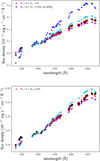 |
Fig. A.1 Same as the bottom of Fig. 5, but for UVES spectrum no. 2 (top) and UVES spectrum no. 3 (bottom). We also show the continuum flux densities when corrected with the veiling flux plus and minus its standard deviation (magenta and cyan asterisks). For the UVES no. 2 spectrum we show additionally the best extinction fit without a veiling flux applied (blue asterisks). |
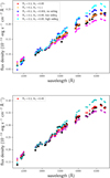 |
Fig. A.2 Same as the bottom of Fig. 5 and Fig. A.1, but for X-Shooter spectra no. 1 (top) and no. 2 (bottom). We also show the continuum flux densities when corrected with the veiling flux plus and minus its standard deviation (magenta and cyan asterisks). For the X-Shooter no. 1 spectrum we show additionally the best extinction fit without a veiling flux applied (blue asterisks) and the best fit with RV deviating from 3.1 as given in the legend. We note that the red asterisks are mainly hidden behind the orange dots. |
Appendix B Overall spectrum and emission lines
We show in Fig. B.1 the three absolute flux calibrated UVES spectra and the two X-Shooter spectra clipped to the wavelength range of the UVES spectra. In Fig. B.3 right panel, we show the Na I D lines with our model spectrum from Sect. 8.2 subtracted, while we show the observed normalised D2 line in Fig. 9 and the D1 line in the left panel. In the two bottom panels we show the Hα line and the Ca II H line blended with the Hϵ line. Finally, in Fig. B.2, we show the He I IRT lines.
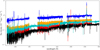 |
Fig. B.1 Absolute flux calibrated spectra of V505 Ori. The three UVES spectra no. 1, 2, and 3 are shown in blue, orange, and red, respectively. The X-Shooter spectrum no. 1 and 2 are shown in black and cyan, respectively. For a better comparison, the two X-Shooter spectra are shown only for the wavelength range of the UVES spectra, which is also the wavelength range we mainly used in our analysis. |
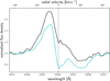 |
Fig. B.2 Continuum-normalised He I IR line as seen in the X-Shooter no. 1 (black) and no. 2 (cyan) spectra. |
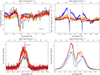 |
Fig. B.3 Same as Fig. 9, but for additional emission lines. Top left: Na I D1 line. Top right: Na I D1 and D2 lines with our spectral model from Sect. 8.2 subtracted. We note that the continua of all spectra are in rough agreement with each other, while the correction in this wavelength range is generally underestimated since the continuum is not located at zero. Such local deviations are expected from a broadband model. Colours are as in Fig. 9: Blue denotes the UVES spectrum no. 1 (brightness maximum), orange spectrum no. 2, red spectrum no. 3, and black the X-Shooter spectrum no. 1 (brightness minimum). Since the photospheric spectrum, the continuum veiling, the reddening, and the grey extinction is subtracted, the emission and absorption seen here must originate from the accretion. We note that the broad absorption feature on the red side can only be seen for the Na I D1 line because of the overlap of the two broad lines. We therefore anchored the velocity scale for its central wavelength marked by the vertical dashed line. Bottom left: Ca II H line blended with the Hϵ line. The broad red absorption feature in the blue and the cyan spectrum are from the radial velocity more compatible to originate from the Hϵ line than from the Ca II H line. Bottom right: Hα line. |
All Tables
Stellar parameters taken from the literature and derived from the data used here.
All Figures
|
Fig. 1 Photometric data around the spectroscopic observations. The different photometric bands are B (blue – HOYS, light blue – AAVSO), V (green – HOYS, light greeen – AAVSO), Rc (red – HOYS, orange – AAVSO), and Ic (black – HOYS, grey – AAVSO). The HOYS R and I band have been shifted by +0.25 and +0.42 mag, respectively, to match the AAVSO data. The vertical grey lines mark the UVES (first three) and X-Shooter (last one) observations. |
| In the text | |
|
Fig. 2 Phase-folded light curve of B, V, R, I band photometry (bottom to top). Colours are as indicated in the legend. Additionally, we show the HOYS U band data in magenta. For clearer display of the brightness maximum we repeat the data and add 1.5 mag in each band except the I band. In the V band we mark with black diamonds the HOYS data taken at the time of the PENELLOPE observations, while the purple square represents HOYS photometry taken near the X-Shooter no. 2 observation. |
| In the text | |
|
Fig. 3 Example of an emission line in the V505 Ori spectrum. The UVES spectra are shown in blue, orange, and red. The two X-Shooter spectra are in black and cyan. The grey spectrum is the PHOENIX spectrum normalised to the first UVES spectrum. The black dashed spectrum is the PHOENIX spectrum with veiling for the UVES spectrum no. 1 added (and again normalised). |
| In the text | |
|
Fig. 4 Relative veiling. The relative veiling is shown for the wavelength range of the UVES spectra determined with the HARPS template star HD 200779. Shown are the mean values of corresponding 150–200 Å chunks in wavelength as dots with the colours indicating the different spectra as given in the legend. The crosses mark the relative veiling as found by Manara et al. (2021). |
| In the text | |
|
Fig. 5 Top: best-fitting AV and RV values for UVES spectrum no. 2. The black dot marks the best-fitting values, and the black, red, and blue contours mark the 68%, 90%, and 95% confidence level. Bottom: comparison of continuum flux density of V505 Ori (black dots) with the veiled and then reddened template (HD 200779) continuum fluxes (red asterisks) for the UVES no. 1 spectrum. |
| In the text | |
|
Fig. 6 V band magnitude of selected cycle epochs. This is illustrating the spread in depth and shape of the individual dimming events in V505 Ori. While the green diamonds mark an especially shallow cycle, the yellow asterisks and blue triangles mark deep cycles. |
| In the text | |
|
Fig. 7 Normalised TESS light curves of V505 Ori in sector 6 and 32. Next to the dominating periodic structure, more details of variability can be seen. For example, in sector 6 there is the additional dip at about day 7, which re-occurs at about day 14. |
| In the text | |
|
Fig. 8 Colour diagram with respect to V band photometry. Red (HOYS) and orange (AAVSO) dots represent V-I, green (HOYS) and light green (AAVSO) dots represent V-R, and blue (HOYS) and light blue (AAVSO) dots represent B-V. The solid coloured lines represent the best linear fit to the data, while the black arrows represent the extinction correction for AV=1.0 mag and RV=3.1. The black symbols denote the mean measurements during the days of the PENELLOPE observations. |
| In the text | |
|
Fig. 9 Examples of emission lines in V505 Ori. The UVES no. 1 spectrum is shown in blue, no. 2 in orange, no. 3 in red, X-Shooter spectrum no. 1 in black, and X-Shooter no. 2 in cyan. As a dashed vertical line, we show the central wavelength of the respective line. Top left: Ca II K line. Top right: Hβ line. Middle left: Mg I line at 5167.32 Å. Middle right: Fe II line at 5316.61 Å. Bottom left: He I D3 line. Bottom right: blue Na I D line at 5889.95 Å. In grey we plot a PHOENIX photospheric spectrum with Teff=4400 K. |
| In the text | |
|
Fig. 10 Best-fitting max and min filling factor of the star spot model for the spot temperature set to 9000 K. The orange dots mark the best-fitting model, and the orange, red, and blue contour lines mark the 68%, 90%, and 95% confidence levels. Colours indicate χ2 as shown by the colour bar. Top: amplitude calculated for photometry taken at the date of UVES spectrum no. 1 and X-Shooter spectrum no. 1. Middle: amplitude calculated for the photometry taken at the date of UVES spectrum no. 1 and 2. Bottom: amplitude calculated for the photometry taken at the date of UVES spectrum no. 2 and X-Shooter spectrum no. 1. Intercomparison of the different panels lead to a spot filling factor for the date of UVES spectrum no. 1 of 18–21%, for no. 2 of 10%, and for the date of the X-Shooter spectrum no. 1 of 3–4%. |
| In the text | |
|
Fig. 11 Scenario for V505 Ori. The vertical black line marks the rotation axis, while the inclined black line marks the viewing horizon on the stellar disk. The dashed blue line marks the magnetic axis. The red lines represent the accretion funnels hitting the star near to the magnetic axis and creating the hot accretion spot there. The (opaque) disk is shown in red here and the dotted black line marks the part of the star, which is blocked from view by the disk. The (asymmetric) pink areas mark less dense parts of the disk, which lead only to reddening of the passing light. Top: brightness maximum. Here, the accretion spot can be fully seen, leading to the highest veiling and some imprint of the accretion funnel in the spectrum. Bottom: brightness minimum. Here, only a small part of the accretion spot can be seen, and the accretion funnel cannot be viewed. |
| In the text | |
|
Fig. A.1 Same as the bottom of Fig. 5, but for UVES spectrum no. 2 (top) and UVES spectrum no. 3 (bottom). We also show the continuum flux densities when corrected with the veiling flux plus and minus its standard deviation (magenta and cyan asterisks). For the UVES no. 2 spectrum we show additionally the best extinction fit without a veiling flux applied (blue asterisks). |
| In the text | |
|
Fig. A.2 Same as the bottom of Fig. 5 and Fig. A.1, but for X-Shooter spectra no. 1 (top) and no. 2 (bottom). We also show the continuum flux densities when corrected with the veiling flux plus and minus its standard deviation (magenta and cyan asterisks). For the X-Shooter no. 1 spectrum we show additionally the best extinction fit without a veiling flux applied (blue asterisks) and the best fit with RV deviating from 3.1 as given in the legend. We note that the red asterisks are mainly hidden behind the orange dots. |
| In the text | |
|
Fig. B.1 Absolute flux calibrated spectra of V505 Ori. The three UVES spectra no. 1, 2, and 3 are shown in blue, orange, and red, respectively. The X-Shooter spectrum no. 1 and 2 are shown in black and cyan, respectively. For a better comparison, the two X-Shooter spectra are shown only for the wavelength range of the UVES spectra, which is also the wavelength range we mainly used in our analysis. |
| In the text | |
|
Fig. B.2 Continuum-normalised He I IR line as seen in the X-Shooter no. 1 (black) and no. 2 (cyan) spectra. |
| In the text | |
|
Fig. B.3 Same as Fig. 9, but for additional emission lines. Top left: Na I D1 line. Top right: Na I D1 and D2 lines with our spectral model from Sect. 8.2 subtracted. We note that the continua of all spectra are in rough agreement with each other, while the correction in this wavelength range is generally underestimated since the continuum is not located at zero. Such local deviations are expected from a broadband model. Colours are as in Fig. 9: Blue denotes the UVES spectrum no. 1 (brightness maximum), orange spectrum no. 2, red spectrum no. 3, and black the X-Shooter spectrum no. 1 (brightness minimum). Since the photospheric spectrum, the continuum veiling, the reddening, and the grey extinction is subtracted, the emission and absorption seen here must originate from the accretion. We note that the broad absorption feature on the red side can only be seen for the Na I D1 line because of the overlap of the two broad lines. We therefore anchored the velocity scale for its central wavelength marked by the vertical dashed line. Bottom left: Ca II H line blended with the Hϵ line. The broad red absorption feature in the blue and the cyan spectrum are from the radial velocity more compatible to originate from the Hϵ line than from the Ca II H line. Bottom right: Hα line. |
| In the text | |
Current usage metrics show cumulative count of Article Views (full-text article views including HTML views, PDF and ePub downloads, according to the available data) and Abstracts Views on Vision4Press platform.
Data correspond to usage on the plateform after 2015. The current usage metrics is available 48-96 hours after online publication and is updated daily on week days.
Initial download of the metrics may take a while.