| Issue |
A&A
Volume 704, December 2025
|
|
|---|---|---|
| Article Number | A202 | |
| Number of page(s) | 17 | |
| Section | Interstellar and circumstellar matter | |
| DOI | https://doi.org/10.1051/0004-6361/202556314 | |
| Published online | 16 December 2025 | |
JWST observations of photodissociation regions
II. Warm molecular hydrogen spectroscopy in the Horsehead nebula
1
Université Paris-Saclay, CNRS,
Institut d’Astrophysique Spatiale,
91405
Orsay,
France
2
Sorbonne Université, CNRS, Institut d’Astrophysique de Paris,
98 bis bd Arago,
75014
Paris,
France
3
Space Telescope Science Institute,
3700 San Martin Drive, Baltimore, MD,
21218,
USA
4
LUX, Observatoire de Paris, Université PSL, Sorbonne Université,
CNRS,
92190
Meudon,
France
5
Université Paris-Cité,
Paris,
France
6
Steward Observatory, University of Arizona,
Tucson,
AZ 85721-0065,
USA
7
Department of Physics & Astronomy, The University of Western Ontario,
London ON N6A 3K7,
Canada
8
Ritter Astrophysical Research Center, University of Toledo,
Toledo,
OH 43606,
USA
9
Sterrenkundig Observatorium, Universiteit Gent,
Krijgslaan 281 S9,
9000
Gent,
Belgium
10
Université Paris-Saclay, Université Paris Cité, CEA, CNRS,
AIM,
91191
Gif-sur-Yvette,
France
11
Leiden Observatory, Leiden University,
PO Box 9513, 2300 RA Leiden,
The Netherlands
12
Faculty of Aerospace Engineering, Delft University of Technology,
Kluyverweg 1, 2629 HS Delft,
The Netherlands
13
UK Astronomy Technology Centre, Royal Observatory Edinburgh, Blackford Hill,
Edinburgh EH9 3HJ,
UK
14
Institut de Recherche en Astrophysique et Planétologie, Université Toulouse III - Paul Sabatier, CNRS, CNES,
9 Av. du colonel Roche,
31028
Toulouse,
France
★ Corresponding author: This email address is being protected from spambots. You need JavaScript enabled to view it.
Received:
8
July
2025
Accepted:
1
October
2025
Abstract
Context. Molecular hydrogen (H2) is the most abundant molecule in the interstellar medium. Because of its excited form in irradiated regions, it is a useful tool for studying photodissociation regions (PDRs), where radiative feedback from massive stars on molecular clouds is dominant. The James Webb Space Telescope (JWST), with its high spatial resolution, sensitivity, and wavelength coverage, provides unique access to the detection of most of the H2 rotational and rovibrational lines, as well as the analysis of their spatial morphology.
Aims. Our goal is to use H2 line emission detected with JWST in the Horsehead nebula to constrain the physical parameters (e.g., extinction, gas temperature, and thermal pressure) throughout the PDR and its geometry.
Methods. We used spectro-imaging data acquired using both the NIRSpec and MIRI-MRS instruments on board JWST to study the H2 spatial distribution at very small scales (down to 0.1′′). From the H2 line ratios, we constrained the extinction throughout the PDR. We then studied the excitation of H2 levels in detail and used this analysis to derive the physical parameters.
Results. We detect hundreds of H2 rotational and rovibrational lines in the Horsehead nebula. The H2 morphology reveals a spatial separation between H2 lines (∼0.5′′) across the PDR interface. Far-ultraviolet (FUV)-pumped lines (v = 0 Ju > 6, v > 0) peak closer to the edge of the PDR than thermalized lines. From H2 lines arising from the same upper level, we estimated the value of extinction throughout the PDR. We find that AV increases from the edge of the PDR to the second and third H2 filaments. We find AV=0.3 ± 1.3 in the first filament and AV=6.1 ± 1.4 in the second and third filaments. We then studied the H2 excitation in different regions across the PDR. The excitation diagrams were fit by two excitation temperatures. As the first levels of H2 are thermalized, the colder temperature corresponds to the gas temperature. The second, hotter component corresponds to the FUV-pumped levels. In each filament, we derive a gas temperature of T ∼500 K. The temperature profile shows that the observed gas temperature remains nearly constant throughout the PDR, with a slight decrease in each of the dissociation fronts. The spatial distribution of H2 reveals that most of the H2 column density is concentrated in the second and third filaments. The column density in the first filament is approximately N(H2)=(3.8 ± 0.8) × 1019 cm−2, while in the second and third filaments it is N(H2)=(1.9 ± 0.4) × 1020 cm−2, about five times higher. The ortho-to-para ratio (OPR) is far from equilibrium, varying from 2–2.5 at the edge of each dissociation front to 1.3–1.5 deeper into the PDR. We observe a clear spatial separation between the para and ortho rovibrational levels, as well as between 0−0 S(2) and 0−0 S(1), indicating that efficient ortho-para conversion and preferential ortho self-shielding are driving the spatial variations of the OPR. Finally, we derive a thermal pressure in the first filament of about Pgas ≥ 6 × 10⁶ K cm−3, which is approximately ten times higher than that of the ionized gas. We highlight that template stationary 1D PDR models cannot account for the intrinsic 2D structure and the very high temperature observed in the Horsehead nebula. We argue that the highly excited, over-pressurized H2 gas at the edge of the PDR interface could originate from mixing between the cold and hot phases induced by photo-evaporation of the cloud.
Conclusions. The analysis of H2 lines detected with JWST provides unique access to the geometry and physical conditions in the Horsehead nebula at very small scales and reveals, for the first time, the possible importance of dynamical effects at the edge of the PDR. This study nevertheless highlights the need for extended modeling of these dynamical effects.
Key words: dust, extinction / HII regions / ISM: lines and bands / ISM: molecules / photon-dominated region / ISM: individual objects: Horsehead
© The Authors 2025
 Open Access article, published by EDP Sciences, under the terms of the Creative Commons Attribution License (https://creativecommons.org/licenses/by/4.0), which permits unrestricted use, distribution, and reproduction in any medium, provided the original work is properly cited.
This article is published in open access under the Subscribe to Open model. This email address is being protected from spambots. You need JavaScript enabled to view it. to support open access publication.
1 Introduction
Photodissociation regions (PDRs) reprocess a significant fraction of the radiation output of young stars by reemitting this energy in the infrared-millimeter wavelength regions through gas lines, aromatic bands, and thermal dust emission. The infrared emission from PDRs dominates the spectra of galaxies and traces the regions where radiative feedback is dominant. This mechanism is a major factor that limits star formation (e.g., Inoguchi et al. 2020) by contributing to cloud dispersal through gas heating and angular momentum addition. Moreover, the intense stellar far-ultraviolet (FUV) radiation incident upon PDRs plays a dominant role in the physics and chemistry of gas and dust (for a review, see Hollenbach & Tielens 1999; Wolfire et al. 2022). The study of these regions is therefore essential for a better understanding of star formation and the evolution of interstellar matter. Moderately excited PDRs, such as the Horsehead nebula, are representative of most of the UV-illuminated molecular gas in the Milky Way and star-forming galaxies. The proximity and almost edge-on geometry of the Horsehead nebula facilitate detailed studies of the physical structures of PDRs and the evolution of the physicochemical characteristics of the gas and dust. The Horsehead is located on the western side of the molecular cloud Orion B at a distance of ∼400 pc (Anthony-Twarog 1982). It emerges from the edge of the L1630 molecular complex and appears as a dark cloud silhouetted against the H II region IC434 (e.g., de Boer 1983; Neckel & Sarcander 1985; Compiègne et al. 2007; Bally et al. 2018). The nebula is illuminated by the O9.5V binary system σ Orionis (Warren & Hesser 1977), most likely on its backside, as it appears in silhouette. This system has an effective temperature of Teff ∼34 600 K (Schaerer & de Koter 1997) and is located at a projected distance of ∼3.5 pc from the edge of the Horsehead PDR. The incident UV field on the PDR is estimated as G0 ∼100 (with G0=1 corresponding to a flux integrated between 91.2 and 240 nm of 1.6 × 10⁻³ erg cm−2 s−1, Habing 1968).
Molecular hydrogen (H2) is the most abundant molecule in galaxies. It forms on the surface of interstellar grains, where the grains act as catalysts (Habart et al. 2004; Bron et al. 2014; Wakelam et al. 2017). During its formation process, it is assumed, considering equipartition, that a third of the energy released by the reaction is converted into the internal energy of the produced H2. The other two-thirds of the H2 formation energy is distributed between grain excitation and the kinetic energy of the released molecules. However, the branching ratio is unknown and the distribution is likely uneven, depending on the conditions in the PDR and the nature of the grains. Additionally, in these regions, the first levels of H2 are excited through collisions owing to the high densities, while highly excited levels are populated by FUV pumping driven by the intense UV field. Molecular hydrogen (H2) is a highly useful tool for studying PDRs. Indeed, as its lowest first levels are thermalized at densities above ≈ 104 cm−3, H2 acts as a thermometer of the medium. Multiple lines of H2 have already been observed in the Horsehead nebula. The pure rotational lines detected with Spitzer have revealed that only the levels v = 0, J<5 are thermalized, while the more highly excited levels are primarily pumped by the UV field (Habart et al. 2011). Consequently, the line intensities of these higher levels do not reflect the gas temperature but rather the fraction of the FUV photon flux pumping H2. Observations of the 1−0 S(1) line with the New Technology Telescope (NTT) revealed bright, narrow filaments at the illuminated edge of the PDR (Habart et al. 2005). Comparisons between observations and PDR models have indicated a steep density gradient at the edge, with a scale length of ≤ 0.02 pc (or ∼10′′) and nH ∼104−cm−3 and nH ∼105 cm−3 in the H2 emitting and inner molecular layers, respectively. Habart et al. (2005) also showed that the Horsehead is viewed with a small inclination of ∼6°, and thus is not strictly edge-on. An important finding from previous H2 observations is that the observed column densities of rotationally excited H2 are much higher than PDR model predictions (Habart et al. 2011). In moderately excited PDRs such as the Horsehead, the discrepancy between the model and the observations is about one order of magnitude for rotational levels Ju ≥ 5. This discrepancy suggests that our understanding of the formation and excitation of H2, and of PDRs heating and/or dynamics, remains incomplete. To address this problem, James Webb Space Telescope (JWST) observations are essential because they allow spatial resolution at the smallest spatial scales and facilitate detection of numerous H2 rotational lines (whereas with Spitzer the detection was limited to a few lines).
Several studies have observed the Horsehead nebula over the years. For instance, observations of CO J = 1−0 have provided an estimate of the mean density of the Horsehead nebula (nH ∼5 × 103 cm−3, Pound et al. 2003). More recently, observations of millimetric molecular emission with the Atacama Large Millimeter/Submillimeter Array (ALMA) at a high angular resolution of ∼0.5′′ revealed a very thin atomic zone, with a size <650 au, suggesting a sharp transition between molecular and ionized gas (Hernández-Vera et al. 2023). From CO data, they also derive the local gas density (nH=(3.9−6.6) × 104 cm−3) and the thermal pressure (Pth=(2.3−4.0) × 106 K cm−3) at a distance of 15′′ from the edge of the cloud, defined as the ionization front.
With its high sensitivity and high spatial resolution, JWST resolves H2 emission at very small scales (up to 0.1′′), providing a more detailed understanding of the Horsehead nebula morphology than previous observations. The observations presented here are part of the JWST Guaranteed Time Observations (GTO) program (ID #1192, PI: Misselt; see Fig. 1). Imaging data analysis is presented in Abergel et al. (2024). The broadband NIRCam filter at 3.35 μ m has revealed a network of faint striated features extending perpendicularly to the PDR front into the H II region. This detection may indicate an entrainment of nanodust particles in the evaporative flow. Maps of the 1−0 S(1) line of H2 obtained with NIRCam reveal numerous sharp substructures on scales as small as 1.5′′. Consistent with Hernández-Vera et al. (2023), the imaging data reveal a very small size of the neutral atomic layer (<100 au). Analysis of broadband filter imaging also shows strong color variations between the illuminated edge and the internal regions, which can be explained by dust attenuation if the Horsehead is illuminated from behind. Dust attenuation appears to be non-negligible over the entire spectral range of JWST. Spectroscopic data analysis presented by Misselt et al. (2025) reveals hundreds of H2 lines, constituting the majority of detected lines in the region.
In this study, we present an analysis of H2 emission detected with JWST. Section 2 describes the observations with the NearInfrared Spectrograph (NIRSpec) and the Mid-Infrared Instrument - Medium Resolution Spectroscopy (MIRI-MRS), as well as the data reduction. Section 3 presents the detected spectral features and examines the spatial morphology of H2 emission. In Sect. 4, we use H2 lines to evaluate the variation of extinction throughout the Horsehead nebula. In Sect. 5, we analyze the excitation of H2 throughout the PDR to derive physical parameters such as the gas temperature and the ortho-to-para ratio (OPR). Finally, Section 6 discusses the results of this study in comparison with template models of the Horsehead nebula.
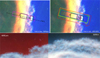 |
Fig. 1 Top panel: JWST NIRCam RGB image of the Horsehead nebula, located in the Orion molecular cloud. Red corresponds to the 3.35 μ m emission (F335M NIRCam filter), blue to the emission of Pa α (F187N filter), and green to the emission of the H2 1−0 S(1) line at 2.12 μ m (F212N filter). Left panel: NIRSpec field of view overlaid on the image in magenta. Right panel: field of view of the different MIRI-MRS channels overlaid on the image (channel 1: blue, channel 2: green, channel 3: yellow, channel 4: red). The black boxes correspond to the aperture used to derive spectra in the dissociation front regions and the dashed black boxes correspond to the aperture in the “molecular” region behind DF1, as defined in Misselt et al. (2025). The dashed line indicates the position of cut #3 from Abergel et al. (2024). Bottom panel: JWST NIRCam and MIRI-MRS composite image of the Horsehead nebula, zoomed on the edge where the faint striated features, attributed to an evaporative flow, are more visible. The image is rotated by 90° with respect to the top panel. Credit: ESA/Webb, NASA, CSA, K. Misselt (University of Arizona), and A. Abergel (IAS/University Paris-Saclay, CNRS). |
2 Observations and data reduction
In this study, we used MIRI-MRS and NIRSpec from the GTO #1192 program. Observations with the MIRI-MRS mode of the Mid-Infrared Instrument (MIRI, Wright et al. 2023) were obtained on May 2, 2024. The MRS covers a total wavelength range from 4.9 to 27.9 μ m, separated into four integral field units (IFU) referred to as channels, each further divided into three bands. The channels have slightly different fields of view (FoVs), from 3.2′′ × 3.7′′ (channel 1) up to 6.6′′ × 7.7′′ (channel 4), and different spatial resolutions (0.19′′ to 0.27′′) and spectral resolutions (∼3700 to ∼1500) (Labiano et al. 2021). The observations cover a strip across the Horsehead filaments at the interface between ionized and molecular gas (see Fig. 1). We used a two-point extended source dither pattern, with 26 groups per integration and one integration per exposure, in FASTR1 readout mode, covering the entire MRS spectral range in three exposures (one per MRS band), with an on-source integration time of 144 s per band. Following the recommended strategy, we obtained a relatively emission-free background observation with the same integration time per band. Although the two-point dither is not the standard recommended strategy, it was adopted as a compromise due to the allocated time in the GTO program. The limited depth of background observations constrains the accuracy of continuum measurements (for more details, see Misselt et al. 2025).
The MIRI-MRS data reduction was performed using the JWST Science Calibration Pipeline (version 1.17.1, Bushouse et al. 2023), with context 1326 of the Calibration Reference Data System (CRDS), following standard procedures (see Labiano et al. 2016; Álvarez Márquez et al. 2023, for detailed examples of MRS data reduction and calibration). Careful examination of the data showed that stage 1 corrections (Morrison et al. 2023) could be run with the default parameters and did not leave significant residuals. We applied the image-to-image background correction in the stage 2 pipeline (Argyriou et al. 2023; Gasman et al. 2023; Patapis et al. 2024). We disabled the master background correction and sky matching steps in stage 3 of the pipeline before producing the final fully reconstructed science cubes (Law et al. 2023), as they introduced artifacts in the data. We then realigned the MRS astrometry using the simultaneous imaging data registered to the Gaia DR3 catalog, resulting in residuals of less than 0.1′′. Finally, we rotated the science cubes to the standard orientation with north up and east to the left, increasing the total FoV in channel 1 to 6.1′′ × 5.6′′ and up to 11.5′′ × 11.5′′ in channel 4.
For NIRSpec, a three-point cycling dither strategy was used. We obtained four groups in NRSIRS2 mode (5 frame coadds per downlinked group), providing a total depth of ∼875 s per pixel in each grating. Dedicated background exposures free of emission, with a configuration identical to a single on-source mosaic pointing, were also acquired for NIRSpec.
The NIRSpec data were processed using the JWST science pipeline version 1.14.0 and the context jwst_1242.pmap of the CRDS. However, the level-1b rate pipeline was slightly modified to account for a subtlety in correctly identifying jumps in grouped data with a small number of groups (see Misselt et al. 2025, for more details). After custom processing, the rate files were reinserted into the pipeline for stage 2 processing. Background subtraction was performed during stage 3.
In the present analysis, we adopt the regions defined in Misselt et al. (2025) to analyze H2 lines. The first defined region, referred to as DF1, corresponds to the first filament, peaking around 2′′ after the front. The second region, DF2, corresponds to the second and third filaments, peaking around 8′′ and 10′′ after the front, respectively (see Fig. 1).
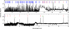 |
Fig. 2 NIRSpec (top) and MIRI-MRS (bottom) spectra averaged over the first filament, DF1. Red and blue lines correspond to the detected rotational and rovibrational transitions of H2, respectively. Most of the lines detected in the dissociation front are attributed to H2. The identification of other lines is provided in Misselt et al. (2025). |
3 Overview of H2 emission in the Horsehead nebula
3.1 Detected lines
We detect hundreds of H2 lines in the Horsehead nebula. Misselt et al. (2025) report pure rotational v = 0−0(J<20) and v = 1−1 (J<20) series, with tentative identifications of isolated v = 2−2, v = 3−3, and v = 4−4 lines. We also detect many rovibrational transitions in the vibrational v = 1−0(J<16), v = 2−1(J<19), v = 2−0(J<8), v = 3−2(J<14), and v = 3−1(J<14) series. Fig. 2 shows a full NIRSpec and MIRI-MRS spectrumaveraged in the first filament, DF1 (see Fig. 1). This figure shows that H2 lines correspond to the majority of lines detected in the dissociation front.
3.2 Morphology of H2 emission
The spectro-imaging capabilities of JWST allow us to study the spatial morphology of H2 emission throughout the Horsehead nebula. To derive the absolute intensities of H2 lines, we fit the observed lines with a Gaussian combined with a linear function to account for the continuum, followed by integration of the Gaussian over the wavelength. We chose not to subtract the continuum to minimize the uncertainty of its estimation on the value of the integrated intensity. Only lines well reproduced by the fitting procedure were retained (i.e., the residuals in the vicinity of the line, after subtraction of the fit, were comparable to or below the noise level in nearby line-free regions). We then produced maps of the brightest H2 lines, with selected examples shown in Fig. 3. This figure presents nine maps: seven from pure rotational transitions and two from rovibrational transitions. The first five maps were obtained with MIRI-MRS, while the last four are derived from NIRSpec. All maps reveal spatial structures with widths greater than ∼1′′, exceeding the PSF width at all wavelengths, indicating that these structures are properly resolved for all lines. As H2 emission traces the dissociation front, where atomic hydrogen becomes molecular, the maps reveal three spatial peaks, corresponding to distinct dissociation fronts. The two brightest peaks, on the left, are separated by ∼2′′ and appear on top of a single filament and are therefore treated as one entity throughout this analysis (designated the DF2 region). These maps indicate that the more highly excited lines (Ju>6) peak closer to the edge of the filaments than the lower-excitation lines.
Fig. 4 shows the normalized intensity profiles of several H2 lines across the PDR along cut #3 (see Fig. 1), averaged over 0.5′′ perpendicular to the cut, as presented in Abergel et al. (2024). This figure confirms the spatial separation of the H2 lines, where the FUV-pumped lines (such as 0−0 S(5), 0−0 S(8) and 1−0 S(1)) peak closer to the edge of the PDR than thermalized lines (such as 0−0 S(1), 0−0 S(3)). This spatial separation (∼0.5′′) arises because the lower rotational levels of H2 have lower energies and can be excited by collisions at lower temperature. However, higher levels of H2 are mostly excited by FUV-pumping. Hence, they peak at the position where the UV field is higher, closer to the edge. This figure also shows that peaks in excited H2 emission precede those of nanograin dust emission. Specifically, aromatic infrared band (AIB) emission at 3.35 μ m (F335M filter of NIRCam) appears correlated with the 0−0 S(1) H2 line.
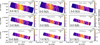 |
Fig. 3 Maps of the brightest H2 rotational lines emission and 1−0 S(1) and 2−1 S(1) rovibrational line emission obtained with MIRI-MRS and NIRSpec across the PDR front. White contours indicate the 0−0 S(1) line emission. |
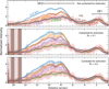 |
Fig. 4 Normalized (around the first peak) intensity profiles across the front (cut #3 of Abergel et al. 2024) averaged over 0.5′′ perpendicular to the line cut. The illuminating star is located on the right. Top panel: intensities not corrected for extinction. Middle and bottom panels: intensities corrected for extinction using the attenuation profile derived in Sect. 4 with a parametrized extinction curve of Gordon et al. (2023) at RV=3.1 (middle) and RV=5.5 (bottom). The filled areas indicate uncertainties, which become particularly important after 15′′ because the extinction estimation is uncertain due to the low signal-to-noise ratio of the NIR lines used. |
4 Evaluation of attenuation by foreground matter
Imaging data from Abergel et al. (2024) show that, in the JWST wavelength range, the detected emission is affected by attenuation effects of the foreground matter. To analyze H2 emission accurately, it is therefore necessary to correct for extinction, which may vary across the field of view.
For optically thin emission, as is the case for H2 lines, the line intensity is directly proportional to the column density of the upper level:
 (1)
where λi j is the line wavelength, Ai j the Einstein coefficient, Nup the upper level column density, h the Planck constant, and c the light velocity. Thus, the ratio of two lines coming from the same upper level (such as 1−0 S(1) and 1−0 Q(3)) depends solely on the wavelengths and the Einstein coefficients, independent of physical conditions. The ratio is given by
(1)
where λi j is the line wavelength, Ai j the Einstein coefficient, Nup the upper level column density, h the Planck constant, and c the light velocity. Thus, the ratio of two lines coming from the same upper level (such as 1−0 S(1) and 1−0 Q(3)) depends solely on the wavelengths and the Einstein coefficients, independent of physical conditions. The ratio is given by
 (2)
As the line is attenuated by dust extinction, the observed intensity is written as follows:
(2)
As the line is attenuated by dust extinction, the observed intensity is written as follows:
 (3)
where AV denotes the visual extinction and Aλ/AV the value of the extinction curve at a wavelength λ. We can therefore derive the visual extinction from the ratios of two H2 lines sharing the same upper level as
(3)
where AV denotes the visual extinction and Aλ/AV the value of the extinction curve at a wavelength λ. We can therefore derive the visual extinction from the ratios of two H2 lines sharing the same upper level as
 (4)
(4)
We derived the visual extinction caused by foreground matter in different regions of the Horsehead nebula using a total of 87 H2 line ratios from the same upper levels. These transitions cover wavelengths from 1.1−4.3 μ m. No sufficiently detected MIR lines with the same upper levels were available for this analysis. Consequently, the attenuation in the NIR biases our estimate of attenuation and no MIR attenuation constraints apply. We used this method to derive the visual extinction initially in the DF1 and DF2 regions, then throughout the PDR. For this, we used the RV-parametrized extinction curve from (Gordon et al. 2023; Gordon et al. 2009; Fitzpatrick et al. 2019; Gordon et al. 2021; Decleir et al. 2022) at RV=3.1, representative of a diffuse medium extinction curve, and RV=5.5, representative of a medium with a depletion of nanograins. In DF1, taking the median of the AV values derived from the H2 lines ratios, we find AV(RV=3.1)=0.3 ± 1.3 and AV(RV=5.5)=0.2 ± 0.5. Due to the low signal-to-continuum ratio of the lines detected in DF1, the dispersion of the values is quite wide, explaining the large uncertainty. Nevertheless, the AV in DF1 is consistent with zero, indicating minimal attenuation in this region. In DF2, we derive AV(RV=3.1)=6.1 ± 1.4 and AV(RV=5.5)=4.5 ± 1.0, indicating that DF2 is significantly more attenuated than DF1. These values derived are consistent with AV estimates from HI recombination lines by Misselt et al. (2025), who find AV=1.51 ± 0.93 in DF1 and AV=7.02 ± 2.60 in DF2.
To estimate the foreground attenuation AV throughout the PDR, we used maps from H2 rovibrational lines. Because these lines are relatively weak, we degraded the spatial resolution of the NIRSpec data cube by averaging the signal along the width of the map and also over four columns of pixels. For each column of pixels, we used all available detected line ratios to derive an AV value. Fig. 5 shows the AV profile across the PDR, calculated using an extinction curve estimated at RV=3.1 along cut #3 of Abergel et al. (2024). The value of AV increases from the first H2 and dust front to the second and third. A similar profile is obtained when using RV=5.5, with AV values being 1.4 times lower. At distances below 1′′ and above 14′′ from the first front, the intensity of H2 drops drastically, making it impossible to estimate the extinction in those regions. This AV profile is also consistent with that derived by Misselt et al. (2025) from HI recombination lines over the same wavelength range (see their Fig. 6).
These results are consistent with the schematic view of the Horsehead geometry shown in Fig. 13 of Abergel et al. (2024), in which the PDR illuminated from behind. The higher extinction in DF2 compared with DF1 indicates that DF2 is located farther from the observer than DF1. This also confirms that the H2 emitting region is much smaller than the depth of the attenuating material. Based on the H2 column density derived in Sect. 5, the emission region of H2 is expected to peak at AV<0.2.
To discriminate between different extinction curves (e.g., RV=3.1 or RV=5.5) in the Horsehead nebula, we employed a χ2 method. We compared the theoretical H2 ratio from Eq. (2) to the observed ratio when corrected for extinction using extinction curves with parameters varying from AV=0−20 and RV: 2−10. We calculated χ2 as
 (5)
where
(5)
where  denotes the extinction-corrected ratio,
  is the theoretical H2 ratio, and σ the uncertainty in the observed ratio1. Fig. 6 demonstrates that RV and AV are highly degenerate, making it impossible to discriminate the extinction curve in the Horsehead nebula. This degeneracy arises because we used only H2 lines in the NIR, which are insufficient to resolve it.
The middle and bottom panels of Fig. 4 show the normalized intensity profiles corrected for extinction using our previous AV estimates with extinction curves from Gordon et al. (2023) at RV=3.1 and RV=5.5. These panels reveal that the derived attenuation does not account for the variation of H2 lines intensity ratios between DF1 and DF2. For thermalized lines (0−0 S(1) and S(3)), these differences can be attributed to temperature variations (see Sect. 5.1). However, we expect the FUV-pumped lines (0−0 S(5), 0−0 S(8) and 1−0 S(1)) to have higher intensities where the column density is higher (i.e., in DF2). The figure shows that while the intensity of the 1−0 S(1) increases by a factor of 2.5 between the first and second filaments, the intensity of the 0−0 S(5) and 0−0 S(8) lines increases by less than a factor of two. Our correction of extinction does not increase the intensity of these lines in DF2. Furthermore, dust profiles at comparable wavelengths (5.5 and 7 μ m) show a second filament three times higher than the first (see Fig. 7 of Abergel et al. 2024). Hence, these characteristics cannot be explained by extinction effects. This suggests that pure rotational levels, even excited, are more sensitive to temperature variations than rovibrational levels. These findings suggest that collisional excitation in the first filament is not negligible for highly excited rotational levels.
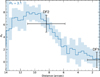 |
Fig. 5 Profile of AV, the attenuation by the foreground matter, across the PDR front, derived from H2 line ratios. The signal was averaged over the width of the maps and four columns of pixels to compute H2 maps with sufficient S/N. Within 1′′ and beyond 14′′ from the front, H2 emission is too faint to derive AV. The value of AV increases from the edge of the PDR to the second and third H2 filaments. |
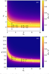 |
Fig. 6 Maps of |

5 Excitation of H2 and physical state of the filaments
5.1 Estimation of the gas temperature
This section discusses the excitation of H2 throughout the PDR. First, we derived the gas temperature within distinct dissociation fronts using the apertures defined in Misselt et al. (2025), namely DF1 and DF2 (see Fig. 1). Fig. 7 presents excitation diagrams of the v = 0 levels of H2 in DF1 and DF2. These excitation diagrams were generated using the PhotoDissociation Region Toolbox Python module2 (pdrtpy; Kaufman et al. 2006; Pound & Wolfire 2008, 2011, 2023). For DF2, the line intensities were corrected for extinction using the RV− parametrized extinction curve of Gordon et al. (2023), with RV=3.1 and AV=6.1, as derived in Sect. 4. In both regions, the excitation diagrams reveal the presence of two distinct temperatures. This indicates that H2 excitation follows two Boltzmann distributions, described by
 (6)
(6)
The slope break occurs at an energy of 6000 K, coinciding with the first levels of v = 1. Since the first levels of H2(J<6) are maintained in thermal equilibrium via collisions, the cold excitation temperature corresponds to the gas temperature. The excitation diagrams presented in Fig. 7 indicate that the observed gas temperature in DF1 is approximately Tobs=512 ± 19 K. In DF2, the observed gas temperature is slightly lower at Tobs= 478 ± 12 K. The difference in gas temperature between the two apertures likely arises because the DF2 front is mixed with the decrease of DF1. Consequently, the high-temperature part of the front is not probed, contrary to DF1. Using Eq. (6), we can also derive the total column density of H2 from the excitation diagrams. The column density is N(H2)=(3.8 ± 0.8) × 1019 cm−2 in DF1 and N(H2)=(1.9 ± 0.4) × 1020 cm−2 in DF2. Thus, the column density of H2 is five times higher in DF2 than in DF1. A summary of the derived parameters is presented in Table 1.
We also derived the gas temperature and column density across the entire MIRI-MRS map using the pdrtpy toolbox. Fitting two temperature components, as in DF1 and DF2, was not possible because the H2 line maps lacked sufficient signal-to-noise ratios. Therefore, we fit the cold component of the excitation diagram in each pixel of MIRI-MRS, using the first four lines of H2 detected with JWST (0−0 S(1)−0−0 S(4)), which are thermalized. The column density and gas temperature maps are shown in Fig. 8. The top panel indicates the highest column density around the second and third filaments (N(H2) ∼5 × 1020 cm−2, with a mean pixel relative error of  ), consistent with the value derived from the excitation diagrams in Fig. 7. The middle panel reveals a modest gas temperature variation across the PDR (from 600 to 380 K), with a mean pixel relative error of
  . This contrasts with the expected attenuation of the UV field and thus the expected temperature decrease (down to ∼100 K) within each filament.
Fig. 9 shows the observed temperature profile along cut #3 of Abergel et al. (2024). This figure reveals that the temperature decreases following the peak of each filament. The temperature derived from the first four H2 lines indicates a decrease from 550 to 400 K in the first filament and from 450 to 400 K in the second and third filaments. The temperatures at the peaks of DF1 and DF2 are similar, at approximately 440 K. The dashed pink line represents the temperature derived from the first three lines (S(1) - S(3)). The estimated temperatures based on either three or four H2 lines are similar at the peak of DF1 and in DF2, but diverge near the front of DF1. At the PDR front, the temperature derived from the first four lines reaches approximately Tobs ∼550 K, while those from the first three lines yield Tobs ∼480 K. This difference indicates the effects of UV pumping on the excitation of the J = 6 level, which may not be thermalized at the front.
Parameters derived from H2 lines in the Horsehead nebula.
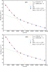 |
Fig. 7 Excitation diagrams in DF1 (top panel) and DF2 (bottom panel). Full excitation diagrams are presented in Appendix B. |
5.2 Spatial variations of the ortho-to-para ratio
Using the pdrtpy module, we also fit the OPR. Fig. 7 shows that the OPR does not reach the equilibrium value of 3 expected for temperatures above 200 K (Sternberg & Neufeld 1999). In both DF1 and DF2, the OPR is ∼2. Fig. 8 presents a map of the OPR in the Horsehead nebula. Overall, the value of the OPR remains below 3 throughout the nebula. The map shows that the OPR reaches its maximum (OPR ∼2−2.5) at the edge of each dissociation front, where the temperature increases. Deeper within the PDR, the OPR decreases to ∼1.3−1.5. These variations are significant, with a mean (resp. median) pixel uncertainty of ∼0.3 (resp. ∼0.06). These OPR values contradict the high temperatures detected, at which equilibrium should be easily reached. This indicates the presence of out-of-equilibrium mechanisms, such as the ortho-para conversion, favoring the formation of para (Bron et al. 2016), or the advection and mixing of colder H2 in the warm region (Gorti & Hollenbach 2002; Störzer & Hollenbach 1998). The latter explanation is in agreement with photoevaporative flows observed in the imaging data, revealing important dynamical effects (Abergel et al. 2024).
Interestingly, we also observe an inversion of the 0−0 S(1) and 0−0 S(2) peaks (top panel, Fig. C.4). These findings confirm the high efficiency of ortho-para conversion, which leads to small OPR inside the PDR, both with gas-phase reactive collisions (as the gas temperature decreases) and dust-surface conversion (as the dust temperature decreases) (Bron et al. 2016). No spatial shift between ortho and para levels is observed for more excited H2 rotational levels, as these originate from warmer regions where the OPR approaches 3. Moreover, the OPR derived from the excited rotational levels (Jup=5−7) is higher and closer to 3 than that of the lowest levels (Jup=3−5). This trend is visible in the excitation diagrams in Fig. 7, where the high J levels are more aligned than the low J levels).
In addition, a different OPR is observed for the rovibrational transitions. As shown in the excitation diagrams, the rovibrational OPR is lower than that for rotational levels (see Fig. B.1). Throughout the mapped region, we find  (Fig. C.2). This behavior is explained by preferential self-shielding of ortho levels relative to para levels. This process favors the pumping of para levels and thus para vibrational transitions (Sternberg & Neufeld 1999). That explains the spatial shift between ortho and para levels in the rovibrational transitions (Figs. C.1, C.3, and the bottom panel of Fig. C.4).
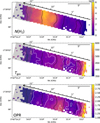 |
Fig. 8 Maps of column density (top panel), gas temperature (middle panel), and ortho-to-para ratio (bottom panel) corrected for extinction. The black contours show the H2 0−0 S(1) line corrected for extinction, with levels of: 4.5 × 10⁻⁵ and 1.5 × 10⁻⁴ erg cm−2 s−1 sr−1). The white contours levels are 400, 420, and 500 K for Tgas and 1.2, 1.5, and 2 for the OPR. The gray boxes overlaid on the map correspond to the region where the extinction is poorly constrained. |
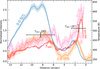 |
Fig. 9 Gas temperature profile derived from the first four observed H2(S(1)−S(4)) lines compared to the H2 0−0 S(1) and 0−0 S(5) line emission profile. The dashed pink line and the dash-dotted pink line correspond to the gas temperature derived from the first three observed lines (S(1) - S(3)) and the first five observed lines (S(1) - S(5)), respectively. A slight decrease in temperature is observed in the H2 filament, while similar temperatures appear at each dissociation front. |
6 Discussion
In the previous section, we derived the temperature profile throughout the PDR. Here, we discuss the resulting estimated thermal pressure and provide brief comparisons with 1D stationary template PDR models to better interpret the observed profile.
6.1 Geometry of the Horsehead nebula
The Horsehead nebula is slightly illuminated on its backside, as depicted in Fig. 10, indicating that it is not observed entirely edge-on. This implies that, regardless of the distance from the edge of the PDR (taken here as the origin), illuminated material is present on the nebula's backside. This geometry accounts for the modest temperature variation within the PDR, which is expected to decrease rapidly between the 0−0 S(5) and 0−0 S(1) peaks. Indeed, because the first rotational levels of H2 are very sensitive to temperature, their emission is dominated by illuminated matter. The observed temperature thus reflects the mean gas temperature in the H2 emitting region. Therefore, it is highly probable that the actual gas temperature at and after the 0−0 S(1) peak is lower.
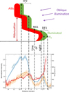 |
Fig. 10 Comparison between a schematic view of the geometry of the Horsehead nebula and the observed H2 and temperature profiles. The figure is adapted from Abergel et al. (2024). |
6.2 Estimate of thermal pressure
Due to the complex geometry of the Horsehead, estimating the local thermal pressure inside the PDR is challenging. Since the observed temperature is dominated by a thin layer of illuminated H2, only the observed temperature at the very edge of the PDR (d<1.5′′, AV ∼0.1), where all gas is illuminated, can be attributed to the local gas temperature.
To estimate the thermal pressure at the PDR edge, we used the measured H2 column density to derive an estimate of the local gas density. At 1.5′′ from the edge, the H2 column density is approximately N(H2) ∼6 × 1018 cm−2. At the edge, we assume that the size of the H2 emission along the line of sight is similar to the distance from the edge toward the star, i.e., approximately 1.5′′. Using this length, we estimate the H2 density as n(H2) ∼6 × 103 cm−3. At this position, the temperature is approximately 480 K. Thus, the H2 thermal pressure is estimated as P(H2)=n(H2) Tgas ∼3 × 10⁶ K cm−3. If all the hydrogen is assumed to be molecular, then n = n(H2) and we can estimate a lower limit of the thermal pressure as Pthlow = nTgas=n(H2)Tgas ∼3 × 10⁶ K cm−3. However, at this distance from the edge, much of the hydrogen is expected to remain atomic or ionized. Therefore, if the emission originates from a region before the H/H2 transition3, then x(H) ≥ x(H2) and n = n(H)+n(H2) ≥ 2 n(H2). Finally, the thermal pressure is at least Pth ≥ 2 n(H2) Tgas ∼6 × 10⁶ K cm−3.
This value is slightly higher than the previous estimates, which are around Pgas ∼(2−4) × 106 K cm−3 (e.g., Habart et al. 2005; Hernández-Vera et al. 2023). This difference can be explained by the fact that the pressure was not measured at the same position in these studies. Hernández-Vera et al. (2023) derive the thermal pressure using CO and HCO+ALMA data at δ x = 15′′ from the edge. At this position, they derive a higher gas density from HCO+ emission, nHCO = (3.9−6.6) × 104 cm−3, than our estimate at the edge (nHH2 ∼104 cm−3). However, from the CO emission, they derive a very low gas temperature, TgasCO = 40−60 K. The cold gas probed deeper within the PDR could have a lower thermal pressure than the hot gas at the edge.
They further derive a thermal pressure by comparing the positions of the H/H2 and the C/CO transitions with PDR models. Their constraints are dH/H2 < 650 au and dC/CO ∼1200 au (see their Fig. 8). Using this method, they derive higher thermal pressures, Pgas=(3.7−9.2) × 106 K cm−3, which are more consistent with our estimate. In addition, JWST observations reveal that the atomic layer is even thinner than expected, with dH/H2 < 100 au (Abergel et al. 2024), indicating high thermal pressures.
The thermal pressure estimate from H2 lines, Pth ≥ 6 × 10⁶ K cm−3, exceeds the predicted pressure in the adjacent H II region IC 434 Pth,HII ≈ ne Te=(2.4−8.0) × 105 cm−3 (Bally et al. 2018). This overpressure, observed between the edge of the PDR and the H II region, may explain the photoevaporative flow observed in the imaging data (Abergel et al. 2024). We discuss this further in Sect. 6.5.
6.3 Comparison with 1D stationary PDR models
To compare observations with stationary 1D PDR models, we used the online grid of isobaric models of the Meudon PDR code4 (Le Petit et al. 2006, version 7). The code simulates the thermal and chemical structure of the gas self-consistently, considering a 1D geometry and a stationary state in a plane-parallel irradiated gas and dust layer. The incident UV radiation field corresponds to that of an O5 star with an intensity of G0=100. The code includes progressive attenuation of the UV field as a result of grain and gas extinction. The extinction curve employed is the mean galactic extinction curve, following the parametrization of Fitzpatrick & Massa (1988).
Figure 11 shows the density and temperature profiles in PDR models at different thermal pressures. This figure demonstrates that these template 1D stationary PDR models, regardless of thermal pressure, cannot reproduce the temperature profile observed in the Horsehead nebula. In the models, the gas temperature always decreases to values well below 400 K inside the PDR. This difficulty in reproducing the temperature profile supports the argument presented in Sect. 6.1 that the temperature derived from H2 lines is not a good tracer of the gas temperature deep inside the PDR, but only reflects the value at the H/H2 transition.
Figure 12 shows the excitation temperature of H2 rotational lines (0−0 S(1) to S(3)) for isobaric PDR models observed face-on at different thermal pressures. Observing face-on means that the observer is at an angle of 0° relative to the normal of the PDR. This corresponds to the integration of line intensities across the entire PDR (AV=0−10). Above AV=0.5, the H2 excitation temperature becomes constant approaching the gas temperature expected at the H/H2 transition (see Fig. 11). Thus, all the H2 emission originates from a thin layer at the edge of the PDR (i.e., before AV=0.5). The H2 lines therefore provide a reliable tracer of the gas temperature in the H2 emitting region. This figure also shows that higher pressure corresponds to higher gas temperatures at the H/H2 transition. For example, the temperature derived from a model at Pth=106 K cm−3 is approximately T ∼200 K, whereas the observed temperature is consistently above 350 K. This result highlights the requirement for high pressure to reproduce the observed temperature using stationary models.
However, even a high-pressure stationary model cannot reproduce the observed excitation diagram. The bottom panel of Fig. 12 shows the excitation diagram in the MO1 region (see Fig. 1), located beyond the 0−0 S(1) peak, approximately 5′′ from the edge, where the line of sight should cross the entire PDR and not only the illuminated edge. The observed temperature in MO1 can therefore be compared to the temperature obtained from modeled H2 lines observed face-on. The temperature observed in this region, approximately Tobs=391 K, is consistently higher than that derived in the models, even at the highest thermal pressure, Pth=3.5 × 10⁷ K cm−3, where Tgas ≈ 314 K. In addition, the overall shape of the excitation diagram differs significantly. In the observations, the H2 column densities are aligned to at least the J = 7 level, indicating that the Boltzmann law at the cold temperature can account for the population distribution of these levels. In the model, the cold temperature accounts only for levels with J ≤ 5. This break in the excitation diagram arises from differences in excitation mechanisms. Fig. 8.20 of Maillard (2023) shows that for a model at Pgas=4 × 10⁶ K cm−3 and G0=100, the collision excitation dominates only for levels with J ≤ 5. For more excited levels, the excitation is dominated by the IR cascade following UV pumping. Previous Spitzer observations of low- to moderately excited PDRs (Habart et al. 2011) have already suggested that models with parameters appropriate for the Horsehead nebula cannot reproduce the observations. This preliminary study suggests that the modeling may lack a heating term that increases the importance of collisional excitation of higher energy levels. This missing heating term could arise from dynamical effects which are not considered in the Meudon PDR code or from the underestimation of microphysical processes. We discuss these effects in the following sections. Further modeling is required to draw firm conclusions and lies beyond the scope of this study.
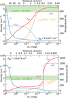 |
Fig. 11 Density (blue) and temperature (red) profiles as a function of AV, the visual extinction within the PDR5 and distance (pc)6 for 1D stationary PDR models with G0=100. Top panel: Pgas=3.5 × 10⁶ K cm−3. Bottom panel: Pgas=3.5 × 10⁷ K cm−3. The dashed gray lines indicate the abundance of H and H2. |
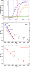 |
Fig. 12 Top panel: excitation temperature derived from the first rotational lines of H2 as a function of AV for face-on isobaric stationary PDR models at different thermal pressures. Middle panel: excitation diagrams derived from the same models as the top panel at AV=1. Bottom panel: excitation diagram observed in MO1, the region behind DF1. |
6.4 Heating processes in stationary PDR models
Figure 13 shows the main heating processes in the PDR models at two different thermal pressures. In both models, the heating processes that dominate at the H/H2 transition are the photoelectric effect on dust grain surfaces and the radiative cascade of H2. In higher-pressure models, the radiative cascade of H2 dominates photoelectric heating before the H/H2 transition. This result may seem counterintuitive, as the abundance of H2 is very low in this region. However, the dissociating efficiency of a photon is about 10 %. Hence, the absorption of a UV photon leads, nine times out of ten, to a radiative cascade into an excited vibrational state. Subsequent collisional de-excitation transfers kinetic energy into the medium, thereby heating the gas. This mechanism becomes more efficient at high density (and thus high pressure), as collisions compete with quadrupolar transitions in the NIR. After the H/H2 transition, the abundance of H2 increases rapidly, so H2 begins to self-shield and the radiative cascade becomes inefficient. This mechanism is then replaced by other processes. The dominant processes include the formation of H2 on dust grains, which releases kinetic energy into the medium, and heating by exothermic chemical reactions that become increasingly important at high thermal pressure. Assessing the relative importance of these processes is essential to identify which term may be underestimated and could lead to the discrepancy between observations and models.
The photoelectric effect is highly efficient on small grains (with radii rd<10 nm, Bakes & Tielens 1994; Weingartner & Draine 2001; Habart et al. 2001). Thus, the significance of this mechanism strongly depends on the abundance of nanograins and their size distribution (Schirmer et al. 2021; Meshaka 2024). For example, Schirmer et al. (2021) demonstrate that nanograin-depleted regions may exhibit lower gas temperatures than regions with ISM-like dust. The evolution of small dust grains at PDR edges, due to the intense UV field, may significantly impact the thermal balance. This could lead models to overestimate or underestimate heating because of the photoelectric effect. Evaluating the dust size distribution remains highly challenging. Using JWST data, Elyajouri et al. (2025) find a similar minimum nanograin size compared to the diffuse ISM but a less steep grain size distribution. Thus, the uncertainty in the extinction curve is a source of uncertainty in the thermal balance, as it influences the location of the H/H2 transition and the local gas temperature at that position.
Additionally, the formation of H2 on dust grain surfaces is poorly constrained (e.g., Habart et al. 2004; Wakelam et al. 2017) and could be a source of underestimation of the gas temperature at the H/H2 transition. In models, equipartition is assumed, so that only one-third of the energy released from the reaction is transformed into kinetic energy. This heating process could be more important if the energy distribution deviates from equipartition. Furthermore, the formation rate of H2 is also badly constrained in PDRs because it depends on the surface area of the small grains. Underestimating the formation rate, which controls the location of the H/H2 transition zone, could shift this transition closer to the PDR edge, where the gas temperature is higher. However, in the low to moderately excited PDR regime, with low G0/nH ratios, H2 self-shields efficiently enough that the H/H2 transition zone already lies closer to the edge.
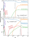 |
Fig. 13 Main heating mechanisms in PDR models at Pgas=3.5 × 10⁶ K cm−3 (top) and Pgas=3.5 × 10⁷ K cm−3 (bottom), with G0=100. |
6.5 Photoevaporation-induced dynamical effects on H2 excitation
We discuss the possibility that the highly pressurized and highly excited H2 detected at the edge of the PDR originates from dynamical effects at the interface between neutral and ionized media. At the edge of the PDR, imaging data reveal a regular pattern of “finger-like” structures resembling small-scale cometary globules observed in photoevaporating molecular clouds (see Fig. 1 and Bertoldi & McKee 1990; Lefloch & Lazareff 1994). Our estimate of the thermal pressure7 derived from H2 lines shows that the PDR front is under higher pressure than the H II region. This suggests that dynamical effects are significant where the intensity of the H2 lines rises steeply, within approximately 1′′ from the ionizing front. This 1′′-scale matches the finger-like structures seen in the imaging data, oriented perpendicular to the interface, and we propose that it corresponds to the scale at which thermal instability develops due to mixing induced by the photoevaporation flow.
The photoevaporation gas flow at the PDR edge triggers advection and mixing between the cold neutral medium (CNM) and the more diffuse neutral and ionized medium, creating turbulent and thermally unstable gas (Bertoldi & Draine 1996; Nakatani & Yoshida 2019). Three-dimensional numerical simulations of turbulent ISM show that mixing between cold and more diffuse gas phases leads to warm and out-of-equilibrium H2, initially formed in the CNM and injected into more diffuse environments (Valdivia et al. 2016; Bellomi et al. 2020; Godard et al. 2023), such as the warm neutral medium (WNM). This mechanism could be responsible for the highly excited H2 we detect at the front. As the temperature in the ionized region (Te ∼8000 K) is significantly higher than that in the PDR, this mixing is likely to yield elevated temperatures at the PDR interface. Hence, this may explain why the observed temperature exceeds that predicted by 1D stationary PDR models, even at high thermal pressure. Constraining the impact of photoevaporation on thermal balance and the formation of these small-scale structures requires detailed numerical modeling using dynamical and thermochemical codes, which lies beyond the scope of this paper.
Another indication of the importance of dynamical effects is that the ionization and dissociation fronts are not clearly spatially resolved and may even be merged (H/H2−IF<100 au), even in high spatial resolution JWST data. Maillard et al. (2021) shows that dynamical effects can significantly reduce the size of atomic layers and even lead to merged fronts. These effects are expected to be particularly significant in low-excitation PDRs such as the Horsehead. In PDRs with low G0/nH, the H2 self-shielding is the dominant source of FUV absorption, compared with dust extinction (Sternberg et al. 2014). This implies that advection of the ionization front has a stronger effect on front merging, as H2 can still be shielded from the UV field. Consequently, lower advection velocities are needed to merge the fronts.
7 Conclusions
In this work, we investigated the spatial morphology and excitation of H2 in the Horsehead nebula. We used H2 lines to constrain the physical parameters of the PDR, including gas temperature and thermal pressure. The main conclusions of this study can be summarized as follows.
We report the first spatial separation between H2 lines peaks d ∼0.5′′. The FUV-pumped lines (v = 0 Ju>6 and v>0) peak closer to the edge than collisionally excited lines (0−0 S(1)-S(4)). The emission of AIBs is more closely correlated with the low-excitation H2 lines than with the FUV-pumped lines.
We derived the attenuation profile across the PDR using rovibrational H2 lines in the near-infrared. The attenuation increases from AV=0.5 at the edge to AV=8 at 12′′ from the edge, assuming RV=3.1. This is consistent with a geometry in which the Horsehead is illuminated on its backside and DF2 lies farther from the observer than DF1.
The H2 column density toward DF2 (N(H2)=1.9 ×..1020 cm−2) is five times higher than toward DF1 (N(H2)=. 3.8 × 1019 cm−2).
The observed temperature derived from H2 lines shows little variation across the PDR, decreasing from 550 K at the edge to 380 K inside the PDR. The slight variation can be explained by the Horsehead not being observed exactly edge-on. If illuminated material is present throughout the field of view, the H2 lines trace the temperature in the illuminated layer and therefore do not reliably trace the gas temperature inside the PDR.
The OPR is not in equilibrium anywhere in the field of view. It varies from OPR ∼2−2.5 at the edges of each dissociation to OPR ∼1.3−1.5 deeper inside the PDR. These variations roughly follow the same trend as the observed temperature, with the OPR reaching its highest value when the temperature is higher.
We used the H2 emission at the very edge of the PDR (d<1.5′′), where all the gas is illuminated, to estimate the thermal pressure. We find a lower limit value around Pgas ≥ 6 × 10⁶ K cm−3, which exceeds the thermal pressure predicted in the H II region.
Template stationary 1D PDR models cannot account for the intrinsic 2D structure and the very high temperatures observed in the Horsehead nebula, which has already been suggested by the previous Spitzer (Habart et al. 2011). This preliminary study suggests that a heating term is missing in the modeling.
We propose that additional heating could originate from mixing between molecular gas and more diffuse atomic and ionized gas at the PDR edge, driven by photoevaporation of the cloud. Detailed modeling is required to link the highly excited and over-pressurized H2 detected in the illuminated filaments at the interface.
In conclusion, our study highlights the complexity of observing cold H2, as its emission is always dominated by illuminated matter within the field of view. Despite this, we derived a very high pressure at the PDR edge, consistent with the photoevaporative flow observed in the imaging data. This observed high pressure implies that the dynamical effects are not negligible in this region. Such effects likely account for the very small size of the atomic layer and the possible merging of the ionized and dissociation fronts, explaining why stationary PDR models fail to reproduce H2 excitation. Dynamical thermochemical models, such as Hydra (Bron et al. 2018), are necessary to constrain the impact of dynamics on the thermal balance and H2 excitation in the Horsehead. To complement the study of dynamics, a detailed analysis of H2 excitation and ortho-para conversion using state-of-the-art PDR models is needed. This will allow for the constraint of specific mechanisms such as ortho-para conversion in the gas and on the dust surface, different self-shielding of ortho and para levels, and potential excitation by cosmic rays in the inner PDR. Deeper observations are needed to better constrain the emission in deeper layers of the PDR, such as the molecular region.
Acknowledgements
This work is based [in part] on observations made with the NASA/ESA/CSA James Webb Space Telescope. The data were obtained from the Mikulski Archive for Space Telescopes at the Space Telescope Science Institute, which is operated by the Association of Universities for Research in Astronomy, Inc., under NASA contract NAS 5-03127 for JWST. These observations are associated with program GTO #1192. This work was performed in part at the French MIRI center with the support of CNES and the ANR-labcom INCLASS between IAS and ACRI-ST, and also supported by the Programme National “Physique et Chimie du Milieu Interstellaire” (PCMI) of CNRS/INSU with INC/INP cofunded by CEA and CNES. K.M. is supported by JWST-NIRCam contract no. NAS5-02015 to the University of Arizona. K.D.G, D.V.D.P., and A.N.-C are partially supported by NASA grant 80NSSC21K1294. M.B. acknowledges funding from the Belgian Science Policy Office (BELSPO) through the PRODEX project “JWST/MIRI Science exploitation” (C4000142239).
References
- Abergel, A., Misselt, K., Gordon, K., et al. 2024, A&A, 687, A4 [NASA ADS] [CrossRef] [EDP Sciences] [Google Scholar]
- Anthony-Twarog, B. J., 1982, AJ, 87, 1213 [NASA ADS] [CrossRef] [Google Scholar]
- Argyriou, I., Glasse, A., Law, D. R., et al. 2023, A&A, 675, A111 [NASA ADS] [CrossRef] [EDP Sciences] [Google Scholar]
- Álvarez Márquez, J., Labiano, A., Guillard, P.,, et al. 2023, A&A, 672, A108 [NASA ADS] [CrossRef] [EDP Sciences] [Google Scholar]
- Bakes, E. L. O., & Tielens, A. G. G. M., 1994, ApJ, 427, 822 [NASA ADS] [CrossRef] [Google Scholar]
- Bally, J., Chambers, E., Guzman, V., et al. 2018, AJ, 155, 80 [Google Scholar]
- Bellomi, E., Godard, B., Hennebelle, P., et al. 2020, A&A, 643, A36 [NASA ADS] [CrossRef] [EDP Sciences] [Google Scholar]
- Bertoldi, F., & Draine, B. T., 1996, ApJ, 458, 222 [NASA ADS] [CrossRef] [Google Scholar]
- Bertoldi, F., & McKee, C. F., 1990, ApJ, 354, 529 [NASA ADS] [CrossRef] [Google Scholar]
- Bron, E., Le Bourlot, J., & Le Petit, F., 2014, A&A, 569, A100 [NASA ADS] [CrossRef] [EDP Sciences] [Google Scholar]
- Bron, E., Le Petit, F., & Le Bourlot, J., 2016, A&A, 588, A27 [NASA ADS] [CrossRef] [EDP Sciences] [Google Scholar]
- Bron, E., Agúndez, M., Goicoechea, J. R., & Cernicharo, J., 2018, ArXiv e-prints [arXiv:1801.01547] [Google Scholar]
- Bushouse, H., Eisenhamer, J., Dencheva, N., et al. 2023, JWST Calibration Pipeline (USA: NASA) [Google Scholar]
- Compiègne, M., Abergel, A., Verstraete, L., et al. 2007, A&A, 471, 205 [NASA ADS] [CrossRef] [EDP Sciences] [Google Scholar]
- de Boer, K. S., 1983, A&A, 125, 258 [Google Scholar]
- Decleir, M., Gordon, K. D., Andrews, J. E., et al. 2022, ApJ, 930, 15 [NASA ADS] [CrossRef] [Google Scholar]
- Elyajouri, M., Abergel, A., Ysard, N., et al. 2025, A&A, 704, A203 [NASA ADS] [CrossRef] [EDP Sciences] [Google Scholar]
- Fitzpatrick, E. L., & Massa, D., 1988, ApJ, 328, 734 [NASA ADS] [CrossRef] [Google Scholar]
- Fitzpatrick, E. L., Massa, D., Gordon, K. D., Bohlin, R., & Clayton, G. C., 2019, ApJ, 886, 108 [Google Scholar]
- Gasman, D., Argyriou, I., Sloan, G. C., et al. 2023, A&A, 673, A102 [NASA ADS] [CrossRef] [EDP Sciences] [Google Scholar]
- Godard, B., Pineau des Forêts, G., Hennebelle, P., Bellomi, E., & Valdivia, V. 2023, A&A, 669, A74 [NASA ADS] [CrossRef] [EDP Sciences] [Google Scholar]
- Gordon, K. D., Cartledge, S., & Clayton, G. C., 2009, ApJ, 705, 1320 [NASA ADS] [CrossRef] [Google Scholar]
- Gordon, K. D., Misselt, K. A., Bouwman, J., et al. 2021, ApJ, 916, 33 [NASA ADS] [CrossRef] [Google Scholar]
- Gordon, K. D., Clayton, G. C., Decleir, M., et al. 2023, ApJ, 950, 86 [CrossRef] [Google Scholar]
- Gorti, U., & Hollenbach, D., 2002, ApJ, 573, 215 [Google Scholar]
- Habart, E., Verstraete, L., Boulanger, F., et al. 2001, A&A, 373, 702 [NASA ADS] [CrossRef] [EDP Sciences] [Google Scholar]
- Habart, E., Boulanger, F., Verstraete, L., Walmsley, C. M., & Pineau Des Forêts, G., 2004, A&A, 414, 531 [NASA ADS] [CrossRef] [EDP Sciences] [Google Scholar]
- Habart, E., Abergel, A., Walmsley, C. M., Teyssier, D., & Pety, J., 2005, A&A, 437, 177 [NASA ADS] [CrossRef] [EDP Sciences] [Google Scholar]
- Habart, E., Abergel, A., Boulanger, F., et al. 2011, A&A, 527, A122 [NASA ADS] [CrossRef] [EDP Sciences] [Google Scholar]
- Habing, H. J., 1968, Bull. Astron. Inst. Netherlands, 19, 421 [Google Scholar]
- Hernández-Vera, C., Guzmán, V. V., Goicoechea, J. R., et al. 2023, A&A, 677, A152 [NASA ADS] [CrossRef] [EDP Sciences] [Google Scholar]
- Hollenbach, D. J., & Tielens, A. G. G. M., 1999, RMP, 71, 173 [CrossRef] [Google Scholar]
- Hwang, J., Pattle, K., Parsons, H., Go, M., & Kim, J., 2023, AJ, 165, 198 [NASA ADS] [CrossRef] [Google Scholar]
- Inoguchi, M., Hosokawa, T., Mineshige, S., & Kim, J.-G., 2020, MNRAS, 497, 5061 [NASA ADS] [CrossRef] [Google Scholar]
- Kaufman, M. J., Wolfire, M. G., & Hollenbach, D. J., 2006, ApJ, 644, 283 [Google Scholar]
- Labiano, A., Azzollini, R., Bailey, J., et al. 2016, SPIE, 9910, 947 [Google Scholar]
- Labiano, A., Argyriou, I., Álvarez Márquez, J.,, et al. 2021, A&A, 656, A57 [NASA ADS] [CrossRef] [EDP Sciences] [Google Scholar]
- Law, D. R., Morrison, J. E., Argyriou, I., et al. 2023, AJ, 166, 45 [NASA ADS] [CrossRef] [Google Scholar]
- Le Petit, F., Nehme, C., Le Bourlot, J., & Roueff, E., 2006, ApJS, 164, 506 [NASA ADS] [CrossRef] [Google Scholar]
- Lefloch, B., & Lazareff, B., 1994, A&A, 289, 559 [NASA ADS] [Google Scholar]
- Maillard, V., 2023, Ph.D. thesis, Université Paris sciences et lettres, France [Google Scholar]
- Maillard, V., Bron, E., & Le Petit, F., 2021, A&A, 656, A65 [NASA ADS] [CrossRef] [EDP Sciences] [Google Scholar]
- Meshaka, R., 2024, Theses, Université Paris sciences et lettres, France [Google Scholar]
- Misselt, K., Witt, A. N., Gordon, K. D., et al. 2025, A&A, 700, A158 [NASA ADS] [CrossRef] [EDP Sciences] [Google Scholar]
- Morrison, J. E., Dicken, D., Argyriou, I., et al. 2023, PASP, 135, 075004 [NASA ADS] [CrossRef] [Google Scholar]
- Nakatani, R., & Yoshida, N., 2019, ApJ, 883, 127 [Google Scholar]
- Neckel, T., & Sarcander, M., 1985, A&A, 147, L1 [Google Scholar]
- Patapis, P., Argyriou, I., Law, D. R., et al. 2024, A&A, 682, A53 [NASA ADS] [CrossRef] [EDP Sciences] [Google Scholar]
- Pound, M. W., & Wolfire, M. G., 2008, ASP Conf. Ser., 394, 654 [Google Scholar]
- Pound, M. W., & Wolfire, M. G., 2011, Astrophysics Source Code Library [record ascl:1102.022] [Google Scholar]
- Pound, M. W., & Wolfire, M. G., 2023, AJ, 165, 25 [NASA ADS] [CrossRef] [Google Scholar]
- Pound, M. W., Reipurth, B., & Bally, J., 2003, AJ, 125, 2108 [NASA ADS] [CrossRef] [Google Scholar]
- Schaerer, D., & de Koter, A., 1997, A&A, 322, 598 [NASA ADS] [Google Scholar]
- Schirmer, T., Habart, E., Ysard, N., et al. 2021, A&A, 649, A148 [NASA ADS] [CrossRef] [EDP Sciences] [Google Scholar]
- Sternberg, A., & Neufeld, D. A., 1999, ApJ, 516, 371 [NASA ADS] [CrossRef] [Google Scholar]
- Sternberg, A., Le Petit, F., Roueff, E., & Le Bourlot, J., 2014, ApJ, 790, 10 [CrossRef] [Google Scholar]
- Störzer, H., & Hollenbach, D., 1998, ApJ, 495, 853 [CrossRef] [Google Scholar]
- Valdivia, V., Hennebelle, P., Gérin, M., & Lesaffre, P., 2016, A&A, 587, A76 [NASA ADS] [CrossRef] [EDP Sciences] [Google Scholar]
- Wakelam, V., Bron, E., Cazaux, S., et al. 2017, Mol. Astrophys., 9, 1 [Google Scholar]
- Warren, Jr., W. H., & Hesser, J. E. 1977, ApJS, 34, 115 [NASA ADS] [CrossRef] [Google Scholar]
- Weingartner, J., & Draine, B., 2001, ApJ, 548, 296 [NASA ADS] [CrossRef] [Google Scholar]
- Wolfire, M. G., Vallini, L., & Chevance, M., 2022, ARAA, 60, 247 [Google Scholar]
- Wright, G. S., Rieke, G. H., Glasse, A., et al. 2023, PASP, 135, 048003 [NASA ADS] [CrossRef] [Google Scholar]

Here, we define the H/H2 transition as the position where x(H)=x(H2).
Grid of isobaric models from August 2024: https://app.ism.obspm.fr/ismdb/
This parameter must not be confused with that displayed in Fig. 5, which represents attenuation by the foreground matter between the H2 emitting region and the observer.
 , with RV=3.1.
The total pressure (including magnetic and turbulent) exceeds the thermal pressure: Ptot=Pth+PB+Pturb. The magnetic pressure can be estimated as  with B = 56 μ G (Hwang et al. 2023). The turbulent pressure can be estimated as
  , where mH is the hydrogen atom mass, μ ∼2 is the mean molecular weight, the gas density is n = 104 cm−3, and the velocity dispersion σv ∼1 km s−1. The turbulent pressure is not negligible in the PDR, as it can reach the same order of magnitude as the thermal pressure. However, given that the H2 lines are not spectrally resolved, the nature of the broadening cannot be determined. We therefore restrict the comparison to estimates of the thermal pressures in the molecular and ionized regions.
Appendix A Comparison between imaging (NIRCam, MIRIm) and spectro-imaging (NIRSpec, MIRI-MRS)
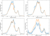 |
Fig. A.1 Comparison of H2 lines and dust emission profiles from imaging data across the front (cut #3 from Abergel et al. 2024) averaged on 0.5′′ perpendicular to the line cut. Profiles are flux-normalized between 0.5 and 3′′ around the first peak. |
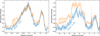 |
Fig. A.2 Comparison of H2 lines and emission profiles from imaging data across the front (cut #3 from Abergel et al. 2024) averaged on 0.5′′ perpendicular to the line cut. Profiles are flux-normalized between 0.5′′ and 3′′ (average around the first peak). |
Appendix B Full excitation diagram
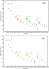 |
Fig. B.1 Total excitation diagram (top) in the DF1 (bottom) in the DF2, apertures defined in Misselt et al. (2025). |
Appendix C Comparison of ortho and para line profile
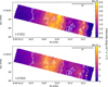 |
Fig. C.1 Comparison of the spatial distribution of an ortho rovibrational line (1−0 S(1)) and a para rovibrational line (1−0 O(2)). White contours are from the 1−0 S(1) line emission. A spatial shift is observed between these lines in the data. |
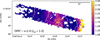 |
Fig. C.2 Ortho-to-para ratio squared map corrected for extinction calculated for v = 1−0 Jup=1−3. White contours are the rotational OPR (levels: 1, 1.5, 2, see Fig. 8). |
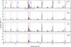 |
Fig. C.3 NIRSpec spectra corrected from extinction between 2 and 3.1 μ m in each of the template region defined in Misselt et al. (2025) (DF: dissociation front, MO: molecular region). The OPR is lower in the “molecular” regions than in the dissociation fronts. |
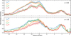 |
Fig. C.4 Normalized intensity (around 0.5 and 3′′ around the first peak) profiles across the front (cut #3 Abergel et al. 2024) averaged on 0.5′′ perpendicular to the line cut. The illuminating star is on the right. (Top) Observed first rotational levels. (Bottom) Observed first rovibrational levels. Para rovibrational levels peaks behind ortho rovibrational levels and the pure rotational para line 0−0 S(2) peaks behind the ortho line 0−0 S(1). |
All Tables
All Figures
|
Fig. 1 Top panel: JWST NIRCam RGB image of the Horsehead nebula, located in the Orion molecular cloud. Red corresponds to the 3.35 μ m emission (F335M NIRCam filter), blue to the emission of Pa α (F187N filter), and green to the emission of the H2 1−0 S(1) line at 2.12 μ m (F212N filter). Left panel: NIRSpec field of view overlaid on the image in magenta. Right panel: field of view of the different MIRI-MRS channels overlaid on the image (channel 1: blue, channel 2: green, channel 3: yellow, channel 4: red). The black boxes correspond to the aperture used to derive spectra in the dissociation front regions and the dashed black boxes correspond to the aperture in the “molecular” region behind DF1, as defined in Misselt et al. (2025). The dashed line indicates the position of cut #3 from Abergel et al. (2024). Bottom panel: JWST NIRCam and MIRI-MRS composite image of the Horsehead nebula, zoomed on the edge where the faint striated features, attributed to an evaporative flow, are more visible. The image is rotated by 90° with respect to the top panel. Credit: ESA/Webb, NASA, CSA, K. Misselt (University of Arizona), and A. Abergel (IAS/University Paris-Saclay, CNRS). |
| In the text | |
|
Fig. 2 NIRSpec (top) and MIRI-MRS (bottom) spectra averaged over the first filament, DF1. Red and blue lines correspond to the detected rotational and rovibrational transitions of H2, respectively. Most of the lines detected in the dissociation front are attributed to H2. The identification of other lines is provided in Misselt et al. (2025). |
| In the text | |
|
Fig. 3 Maps of the brightest H2 rotational lines emission and 1−0 S(1) and 2−1 S(1) rovibrational line emission obtained with MIRI-MRS and NIRSpec across the PDR front. White contours indicate the 0−0 S(1) line emission. |
| In the text | |
|
Fig. 4 Normalized (around the first peak) intensity profiles across the front (cut #3 of Abergel et al. 2024) averaged over 0.5′′ perpendicular to the line cut. The illuminating star is located on the right. Top panel: intensities not corrected for extinction. Middle and bottom panels: intensities corrected for extinction using the attenuation profile derived in Sect. 4 with a parametrized extinction curve of Gordon et al. (2023) at RV=3.1 (middle) and RV=5.5 (bottom). The filled areas indicate uncertainties, which become particularly important after 15′′ because the extinction estimation is uncertain due to the low signal-to-noise ratio of the NIR lines used. |
| In the text | |
|
Fig. 5 Profile of AV, the attenuation by the foreground matter, across the PDR front, derived from H2 line ratios. The signal was averaged over the width of the maps and four columns of pixels to compute H2 maps with sufficient S/N. Within 1′′ and beyond 14′′ from the front, H2 emission is too faint to derive AV. The value of AV increases from the edge of the PDR to the second and third H2 filaments. |
| In the text | |
|
Fig. 6 Maps of |
| In the text | |
|
Fig. 7 Excitation diagrams in DF1 (top panel) and DF2 (bottom panel). Full excitation diagrams are presented in Appendix B. |
| In the text | |
|
Fig. 8 Maps of column density (top panel), gas temperature (middle panel), and ortho-to-para ratio (bottom panel) corrected for extinction. The black contours show the H2 0−0 S(1) line corrected for extinction, with levels of: 4.5 × 10⁻⁵ and 1.5 × 10⁻⁴ erg cm−2 s−1 sr−1). The white contours levels are 400, 420, and 500 K for Tgas and 1.2, 1.5, and 2 for the OPR. The gray boxes overlaid on the map correspond to the region where the extinction is poorly constrained. |
| In the text | |
|
Fig. 9 Gas temperature profile derived from the first four observed H2(S(1)−S(4)) lines compared to the H2 0−0 S(1) and 0−0 S(5) line emission profile. The dashed pink line and the dash-dotted pink line correspond to the gas temperature derived from the first three observed lines (S(1) - S(3)) and the first five observed lines (S(1) - S(5)), respectively. A slight decrease in temperature is observed in the H2 filament, while similar temperatures appear at each dissociation front. |
| In the text | |
|
Fig. 10 Comparison between a schematic view of the geometry of the Horsehead nebula and the observed H2 and temperature profiles. The figure is adapted from Abergel et al. (2024). |
| In the text | |
|
Fig. 11 Density (blue) and temperature (red) profiles as a function of AV, the visual extinction within the PDR5 and distance (pc)6 for 1D stationary PDR models with G0=100. Top panel: Pgas=3.5 × 10⁶ K cm−3. Bottom panel: Pgas=3.5 × 10⁷ K cm−3. The dashed gray lines indicate the abundance of H and H2. |
| In the text | |
|
Fig. 12 Top panel: excitation temperature derived from the first rotational lines of H2 as a function of AV for face-on isobaric stationary PDR models at different thermal pressures. Middle panel: excitation diagrams derived from the same models as the top panel at AV=1. Bottom panel: excitation diagram observed in MO1, the region behind DF1. |
| In the text | |
|
Fig. 13 Main heating mechanisms in PDR models at Pgas=3.5 × 10⁶ K cm−3 (top) and Pgas=3.5 × 10⁷ K cm−3 (bottom), with G0=100. |
| In the text | |
|
Fig. A.1 Comparison of H2 lines and dust emission profiles from imaging data across the front (cut #3 from Abergel et al. 2024) averaged on 0.5′′ perpendicular to the line cut. Profiles are flux-normalized between 0.5 and 3′′ around the first peak. |
| In the text | |
|
Fig. A.2 Comparison of H2 lines and emission profiles from imaging data across the front (cut #3 from Abergel et al. 2024) averaged on 0.5′′ perpendicular to the line cut. Profiles are flux-normalized between 0.5′′ and 3′′ (average around the first peak). |
| In the text | |
|
Fig. B.1 Total excitation diagram (top) in the DF1 (bottom) in the DF2, apertures defined in Misselt et al. (2025). |
| In the text | |
|
Fig. C.1 Comparison of the spatial distribution of an ortho rovibrational line (1−0 S(1)) and a para rovibrational line (1−0 O(2)). White contours are from the 1−0 S(1) line emission. A spatial shift is observed between these lines in the data. |
| In the text | |
|
Fig. C.2 Ortho-to-para ratio squared map corrected for extinction calculated for v = 1−0 Jup=1−3. White contours are the rotational OPR (levels: 1, 1.5, 2, see Fig. 8). |
| In the text | |
|
Fig. C.3 NIRSpec spectra corrected from extinction between 2 and 3.1 μ m in each of the template region defined in Misselt et al. (2025) (DF: dissociation front, MO: molecular region). The OPR is lower in the “molecular” regions than in the dissociation fronts. |
| In the text | |
|
Fig. C.4 Normalized intensity (around 0.5 and 3′′ around the first peak) profiles across the front (cut #3 Abergel et al. 2024) averaged on 0.5′′ perpendicular to the line cut. The illuminating star is on the right. (Top) Observed first rotational levels. (Bottom) Observed first rovibrational levels. Para rovibrational levels peaks behind ortho rovibrational levels and the pure rotational para line 0−0 S(2) peaks behind the ortho line 0−0 S(1). |
| In the text | |
Current usage metrics show cumulative count of Article Views (full-text article views including HTML views, PDF and ePub downloads, according to the available data) and Abstracts Views on Vision4Press platform.
Data correspond to usage on the plateform after 2015. The current usage metrics is available 48-96 hours after online publication and is updated daily on week days.
Initial download of the metrics may take a while.