| Issue |
A&A
Volume 704, December 2025
|
|
|---|---|---|
| Article Number | A149 | |
| Number of page(s) | 21 | |
| Section | Interstellar and circumstellar matter | |
| DOI | https://doi.org/10.1051/0004-6361/202556572 | |
| Published online | 15 December 2025 | |
Multi-scale view of the S-shaped high-mass star-forming filament IRAS 19074+0752 observed as part of the INFANT survey
1
School of Physics and Astronomy, Yunnan University,
Kunming
650091,
PR China
2
Shanghai Astronomical Observatory, Chinese Academy of Sciences,
80 Nandan Road,
Shanghai
200030,
PR China
3
State Key Laboratory of Radio Astronomy and Technology,
A20 Datun Road, Chaoyang District,
Beijing
100101,
PR China
4
National Astronomical Observatory of Japan,
2-21-1 Osawa, Mitaka,
Tokyo
181-8588,
Japan
5
Department of Physics, National Sun Yat-Sen University,
No. 70, Lien-Hai Road, Kaohsiung City
80424,
Taiwan,
ROC
6
Center for Astrophysics, Harvard & Smithsonian,
MS-42, 60 Garden Street,
Cambridge,
MA 02138,
USA
7
National Astronomical Observatories, Chinese Academy of Sciences,
Beijing
100101,
PR China
8
Max Planck Institute for Astronomy,
Konigstuhl 17,
69117
Heideberg,
Germany
9
Instituto de Radioastronomía y Astrofísica, Universidad Nacional Autónoma de México,
Morelia,
Michoacán 58089,
México
10
Department of Astronomy, The University of Tokyo,
Hongo,
Tokyo 113-0033,
Japan
11
Department of Astronomy, Xiamen University,
Zengcuo’an West Road,
Xiamen
361005,
PR China
12
Kavli Institute for Astronomy and Astrophysics, Peking University,
Beijing
100871,
PR China
13
Max-Planck-Institut für Extraterrestrische Physik,
Giessenbachstr. 1,
85748
Garching bei München,
Germany
14
School of Astronomy and Space Science, Nanjing University,
163 Xianlin Avenue,
Nanjing
210023,
PR China
15
Key Laboratory of Modern Astronomy and Astrophysics (Nanjing University), Ministry of Education,
Nanjing
210023,
PR China
16
Department of Earth and Planetary Sciences, Institute of Science Tokyo,
Meguro, Tokyo
152-8551,
Japan
17
Joint Alma Observatory (JAO),
Alonso de Córdova 3107, Vitacura,
Santiago,
Chile
★ These authors contributed equally to this work.
★★ Corresponding authors: This email address is being protected from spambots. You need JavaScript enabled to view it.
; This email address is being protected from spambots. You need JavaScript enabled to view it.
; This email address is being protected from spambots. You need JavaScript enabled to view it.
Received:
24
July
2025
Accepted:
9
October
2025
Abstract
Context. It is generally accepted that high-mass stars form through a hierarchical, multi-scale fragmentation process that range from molecular clouds down to individual protostars, involving intermediate scales such as filaments. However, a comprehensive understanding of this process remains limited due to the lack of high-resolution, multi-scale observational studies that would simultaneously probe the physical conditions across the full hierarchy of star-forming structures.
Aims. We aim to understand a coherent picture of the physical processes connecting filament formation, fragmentation, and dynamical scenario of high-mass star formation in the IRAS 19074+0752 (hereafter I19074) region.
Methods. Primarily using new 1.3 mm continuum mosaicked observations, as part of the ALMA-INFANT survey, we analyzed the S-shaped filamentary cloud I19074 at a ∼6000 AU resolution. Leveraging the multi-scale information, we investigated the filament and clump fragmentation properties, such as core separations and masses.
Results. ALMA 1.3 mm dust continuum emission reveals that the S-shaped filament consists of two physically connected components: a southern (Fs) and a northern (Fn) segment. Fn is associated with an infrared (IR)-bright HII region, while Fs appears IR-dark. The total filament length is ∼2.8 pc, with Fn and Fs spanning ∼1.0 pc and ∼1.8 pc, respectively. Their masses are ∼250−910 M⊙, while their line masses (∼250−360 M⊙ pc−1) exceed the critical value for turbulence support, indicating they are gravitationally bound. The S-shaped morphology likely results from the expansion of the HII region, which swept up and compressed the northern part of the pre-existing filament into an arc-like structure in Fn; meanwhile, Fs retained a more linear form due to its greater distance from the ionized gas. Accordingly, a hybrid scenario could be responsible for Fn formation, which would combine the compression of a preexisting filament by the HII region with fresh gas accumulation into the shocked-compression layer. We extracted 26 dense cores from 1.3 mm emission with masses between 1.0 and 22.9 M⊙, with most (92%) being gravitationally bound (αvir ≤ 2). The core separations lack periodicity; instead, four core groups define four clumps (clumps 1-4) with masses of 110−620 M⊙. In the Fs segment, clump 1 at its southern end could be a product of edge fragmentation, while Fn exhibits hierarchical fragmentation modes: the filamentary mode responsible for clump formation within Fn and the spherical Jeans-like mode for core formation within clumps. Hierarchical fragmentation mechanisms are identified as shocked turbulence-driven within Fn and gravity-driven inside the clumps. Most cores have high mass surface densities of Σcore ≥ 1 g cm−2, but with no robust identification of high-mass prestellar candidates. This favors dynamical clump-fed accretion-type over core-fed accretion-type models for high-mass star formation in I19074.
Conclusions. The S-shaped filament in the I19074 region likely formed through the interaction with an expanding H II region, with the shocked-shell fragmentation mechanism in Fn and edge fragmentation in Fs serving as pathways for producing massive, star-forming clumps. Both mechanisms contribute to high-mass star formation via a dynamical clump-fed accretion process within their respective filamentary segments.
Key words: stars: formation / ISM: clouds / HII regions / ISM: individual objects: IRAS 19074+0752
© The Authors 2025
 Open Access article, published by EDP Sciences, under the terms of the Creative Commons Attribution License (https://creativecommons.org/licenses/by/4.0), which permits unrestricted use, distribution, and reproduction in any medium, provided the original work is properly cited.
This article is published in open access under the Subscribe to Open model. This email address is being protected from spambots. You need JavaScript enabled to view it. to support open access publication.
1 Introduction
The formation mechanism of high-mass stars (M*>8 M⊙) remains an open question in astrophysics. It has been generally accepted that high-mass stars form in stellar clusters, likely through a hierarchical, multi-scale fragmentation process that spans from molecular clouds down to individual protostars, passing through filaments, clumps, and dense cores (Zhang et al. 2009; Wang et al. 2011; Liu et al. 2012b; Zhang et al. 2015; Beuther et al. 2018; Yuan et al. 2018; Vázquez-Semadeni et al. 2019; Chen et al. 2019; Li et al. 2019, 2020; Padoan et al. 2020; Kumar et al. 2020; Liu et al. 2022b,a; Saha et al. 2022; Hacar et al. 2023; He et al. 2023; Yang et al. 2023; Pan et al. 2024; Liu et al. 2023; Luo et al. 2024a,b). Within this paradigm, molecular filaments serve as critical “conveyor belts”, facilitating the transport of gas between large-scale cloud structures and compact star-forming cores (e.g., Galván-Madrid et al. 2010; Liu et al. 2012a; Longmore et al. 2014; Vázquez-Semadeni et al. 2019; Padoan et al. 2020; Kumar et al. 2020; Liu et al. 2023; Álvarez-Gutiérrez et al. 2024; Sandoval-Garrido et al. 2025). Consequently, the formation and evolution of filaments could play a critical role in setting the final mass budget available for high-mass star formation.
The study of molecular filaments has been a central topic in star formation research since their ubiquity was widely revealed over a decade ago through, for instance, Herschel’s wide-field far-infrared (IR) dust continuum observations (André et al. 2010; Molinari et al. 2010). These observations also established a robust empirical correlation between filamentary structures and star formation across a wide range of stellar masses (André et al. 2019; Arzoumanian et al. 2019). Despite this progress, the physical mechanisms responsible for filament formation remain poorly understood. Numerical simulations have shown that filamentary structures can arise in diverse environments, with or without the inclusion of turbulence, magnetic fields, or self-gravity (e.g., Gómez & Vázquez-Semadeni 2014; Smith et al. 2014; Van Loo et al. 2014; Kirk et al. 2015; Federrath et al. 2016; Liu et al. 2025), leaving the dominant formation mechanism(s) still uncertain. Molecular filaments could form either through gravitational fragmentation on cloud scales or via direct compression by interstellar turbulence. For example, in global hierarchical collapse (GHC; Vázquez-Semadeni et al. 2019) model, filaments are envisioned as dynamically evolving structures that continuously accrete gas from their surroundings while simultaneously feeding dense cores embedded within them. In this scenario, gravity is the primary driver of filament formation and evolution (see also Gómez & Vázquez-Semadeni 2014; Vázquez-Semadeni et al. 2017). Alternatively, in models that do not invoke large-scale gravitational collapse, such as the inertial inflow model (Padoan et al. 2020), inertial supersonic flows combined with local self-gravity can produce similarly dynamic filaments. Here, filaments initially form due to shock-compressed velocity-coherent structures driven by turbulence, with gravity subsequently acting to further contract and fragment these newly formed filaments. Beyond turbulence, other physical agents such as magnetic fields and stellar feedback can also contribute to filament formation. Magnetic fields, depending on their strength relative to the gas dynamics, can facilitate filament formation through various mechanisms (e.g., Soler & Hennebelle 2017). Additionally, feedback-driven filaments have been identified at the boundaries of H II regions, as traced by high-sensitivity observations of atomic carbon ([C I]; Pabst et al. 2020) and molecular gas (CO; Suri et al. 2019). In real molecular clouds, filaments could be shaped by a combination of gravity, turbulence, feedback, and/or magnetic fields, with their exact formation pathway depending on local environmental conditions. Investigating the interplay between filaments and their surrounding environments is therefore necessary for disentangling the relative contributions of these physical processes and for elucidating the detailed mechanisms of filament formation.
Filament fragmentation represents a key evolutionary stage through which filaments evolve into dense cores, the sites where stars form. The physical properties of the resulting fragments, such as their mass and density, could determine the final stellar masses, particularly in the case of high-mass stars. Standard semi-analytic cylinder fragmentation models, which assume isolated filaments in hydrostatic equilibrium without turbulence or magnetic fields, predict formation of quasi-periodic chains of dense cores along the filament axis, with a characteristic core spacing of about four times the filament width (e.g., Inutsuka & Miyama 1992). A few examples exhibiting quasi-periodic core distributions have been observed in several filaments (Zhang et al. 2009; Tafalla & Hacar 2015; Liu et al. 2018; Zhang et al. 2020). However, observational studies generally found that the separations between filament-rooted dense cores are non-periodic (e.g., André et al. 2014; Könyves et al. 2020; Yang et al. 2024). This inconsistency between observations and simple theoretical predictions likely stems from the fact that real molecular filaments are not isolated structures in perfect hydrostatic equilibrium (Clarke et al. 2017; Pineda et al. 2023). Therefore, investigating the dynamic environments surrounding filaments is essential for gaining deeper insights into the physical processes governing filament fragmentation into cores and, ultimately, stars.
In this study, we focus on the high-mass star-forming region IRAS 19074+0752 (hereafter, I19074). This region hosts an S-shaped molecular filament extending roughly north-south and is adjacent to an IR bubble in the filament’s northern part (see Fig. 1). The IR bubble is shaped by 8 μm radiation with an angular radius of 18.5′′ (Jayasinghe et al. 2019), corresponding to emission from the two prominent polycyclic aromatic hydrocarbon (PAH) bands at 7.7 and 8.6 μm. These PAH features are good tracers of photodissociation regions (PDRs) that delineate the ionization front created by high-mass stars (Liu et al. 2015, 2018). Indeed, the IR bubble is spatially associated with a classical H II region, likely ionized by one or more O8-O8.5 main sequence stars, as inferred from 20 cm radio continuum observations that trace free-free emission (see Appendix E for details). The systemic velocity of the H II region is 53.4 km s−1 (Anderson et al. 2014), which is close to that of the associated molecular filament (55.5 km s−1; Lu et al. 2018; Cheng et al. 2024). Two kinematic distances for I19074 have been reported based on the rotation curve model of Reid et al. (2009): a near distance of 3.8 kpc (Lu et al. 2018; Cheng et al. 2024) and a far distance of 8.9 kpc (Anderson et al. 2014; Jayasinghe et al. 2019). In this work, we have adopted the far distance of 8.9 kpc, as Anderson et al. (2014) resolves the kinematic distance ambiguity (KDA) through the detection of molecular absorption of the H2 CO line against the background H II region, providing a more reliable distance measurement.
The S-shaped filament is clearly detected in the 1.2 mm single-dish dust continuum map (solid white contours in Fig. 1) with an angular resolution of 11′′. It spans a physical length of 3.5 pc and has a total mass of 1.1 × 10³ M⊙, and a luminosity of 8.8 × 10⁴ L⊙ (Lu et al. 2018; Cheng et al. 2024), all these parameters scaled to the adopted distance. Submillimeter Array (SMA) 1.3 mm dust continuum observations at an angular resolution of 3.5″ by Lu et al. (2018) identified five compact sources along the filament, with masses ranging from 27 to 187 M⊙ (scaled to the adopted distance), one of which is associated with an ultra-compact (UC) H II region (see the plus symbol in Fig. 1). These observations confirm that I19074 is an active site of high-mass star formation.
This paper investigates a comprehensive picture of the physical processes connecting filament formation and fragmentation to dynamical formation of high-mass stars in the 119074 region, primarily using data from the ALMA-INFANT survey (see Sect. 2). The investigation is aimed to provide insights onto the relationships between these different physical processes. Section 2 describes the observational data used in this study. Section 3 presents the results and their analysis. Section 4 discusses the implications of our major findings for scenarios of filament formation, evolution, and high-mass star formation in I19074. Finally, Section 5 summarizes the major results and presents our conclusions.
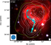 |
Fig. 1 Spitzer three-color image of the I19074 region in the mid-infrared bands (blue: 3.6 μm, green: 4.5 μm, red: 8.0 μm). The white contours represent 1.2 mm dust continuum emission from the MAMBO survey (Beuther et al. 2002), while the black contours indicate 20 cm radio continuum emission from the EFFLSBRG survey (Winkel et al. 2016). Contour levels for the 20 cm radio emission (black) start at 5 σ20 cm(σ20 cm=0.2 mJy beam−1) and increase in steps of 5 σ20 cm. The 1.2 mm dust emission (white) is contoured at [3, 5, 7, 9, 15, 21, 27, 33] × σ1.2 mm, where σ1.2 mm=7 mJy beam−1. Cyan circles and blue plus mark the positions of identified compact sources and UC H II region by Lu et al. (2018). The cyan band outlines the S-shaped filament connecting the compact sources. The (synthesized) beams for the MAMBO (11′′ × 11′′) and ALMA (0.60′′ × 0.58′′) observations are shown in the lower-left and lower-right corners, respectively. The dashed loop shows the ALMA mosaic field. A scale bar of 0.5 pc is shown in the top right corner. |
2 Observations
I19074 was observed as part of the INvestigations of Massive Filaments ANd Star Formation (INFANT) survey (Project ID 2017.1.00526.S, PI: Lu, X.; Cheng et al. 2024) at 1.3 mm during ALMA Cycle 5. The I19074 region was mosaicked (see the mosaic field in Fig. 1) between March and August 2018 using 45 pointing observations with the ALMA C43-1 and C43-4 12 m array configurations, achieving a maximum recoverable scale of 12.4′′. The observation data were calibrated and sequentially imaged with the CASA software package version 6.7.0 (McMullin et al. 2007; CASA Team et al. 2022), where the continuum image centred at 230 GHz was cleaned in an aggregated 3.75 GHz frequency bandwidth free of line emission. Observational details and data reduction were described in Cheng et al. (2024). We primarily made use of the reduced continuum data, which have a synthesized beam of 0.60′′ × 0.58′′ (corresponding to ∼6000 AU at the source distance) and a sensitivity of ∼0.08 mJy beam−1 (equivalent to 0.17 M⊙ at 15 K dust temperature). The INFANT survey also acquired 1.3 mm line data for several major molecular species, such as H2 CO (30,3−20,2) /(32,2−22,1) /(32,1−22,0), SiO(5−4), CO(2−1), and N2 D+(3−2). The reduced data of these lines have a typical sensitivity of 4 mJy beam−1 channel−1, with a synthesized beam of 0.71′′ × 0.66′′ and a channel width of 0.63−0.67 km s−1.
To recover the flux density on extended angular scales, we employed the Miriad-based (Sault et al. 1995) procedure, ALMICA1, which was initially developed for combining an 157-pointings mosaic of the Submillimeter Array (SMA) with the bolometric 850 μm image taken with the James Clerk Maxwell Telescope (JCMT) SCUBA instrument (Liu et al. 2013). It non-linearly combined the ALMA 1.3 mm continuum data with the MAMBO 1.2 mm continuum image that is 11′′ in beam size (Beuther et al. 2002). First, it scaled the flux density in the MAMBO image to the observing frequency of our ALMA observations, assuming a spectral index of 2. It then deconvolved the flux-rescaled MAMBO image to produce an image model that was corrected for the effect of the primary beam of the IRAM-30m telescope. Afterwards, this procedure produced a visibility model for the deconvolved MAMBO image by sampling the image in the Fourier domain over the u v distance range of 0−12 k λ. We did not utilize the full 0−25 k λ u v distance range provided by the IRAM-30 m telescope, since the observations at short u v distances are better immune to deconvolution errors. Finally, it jointly imaged the visibility model for the MAMBO image and the ALMA data, to produce the combined 1.3 mm continuum image. The image was Robust=0.5 weighted, which yielded a 0.64′′ × 0.61′′ synthesized beam (P.A. −1.2°) and an rms noise of ∼0.15 mJy beam−1. The resulting combined continuum image recovers approximately 99% of the total flux measured from the MAMBO map within the area defined by a level of pblimit=0.5 in the ALMA image.
We also employed the line data of NH3 transitions at ∼24 GHz from the Very Large Array (VLA) observations by Lu et al. (2014) for kinematics analysis of the I19074 region. The typical rms achieved is 1.6 mJy beam−1 at a 0.62 km s−1 velocity resolution with a synthesized beam size of 4′′ × 3′′. Details on the VLA observations are referred to Lu et al. (2014). Additionally, ancillary archival data were utilized to analyze the surrounding environment toward I19074. Spitzer 3.6, 4.5, and 8.0 μm images were retrieved from the Galactic Legacy Infrared Midplane Survey Extraordinaire survey (i.e., GLIMPSE, Benjamin et al. 2003). They have angular resolutions better than 2.4″ (Benjamin et al. 2003). Besides, 20 cm radio continuum data were obtained from the Effelsberg-Bonn HI Survey with a synthesized beam size of 6.4′′ × 5.4′′ (Winkel et al. 2016).
3 Results and analysis
3.1 Identification of hierarchical density structures
3.1.1 Identification of filamentary segments
Figure 2 presents the 1.3 mm continuum maps of I19074, with the combined image on the left and the ALMA-alone one on the right. Both maps reveal an overall S-shaped filament, consistent with the 1.2 mm single-dish MAMBO observations (solid white contours in Fig. 1). As outlined in Fig. 2 by the 2 σ1.3 mm, com contour of the combined image (σ1.3 mm, com = 0.15 mJy beam−1), the S-shaped filament comprises two major components: the northern Fn and southern Fs filamentary segments. The lengths of the S-shape, Fn and Fs were accordingly measured to be 2.8 pc, 1.8 pc and 1.0 pc, respectively (see Table 1). We note that the new measurement of the S-shape length from ALMA 1.3 mm continuum emission is slightly shorter than that from the SMA 1.3 mm emission by Lu et al. (2018), which can be understood due to the different maximum recoverable scales between the two different observations. In addition, if the filamentary structures are inclined relative to the plane of the sky by an angle, φ, their actual length will be underestimated in projection by a factor of 1/cos (φ). The inclination of the S-shaped filament is unlikely to be close either to the line of sight or to the plane of sky, as such orientations would make the filament morphology or the velocity gradient along the filament (see Fig. A) not observable to us. We therefore assumed φ ∼45° for the S-shape filament. This assumption leads to the deprojected lengths of ∼4.0 pc, ∼2.5 pc, and ∼1.4 pc for the S-shaped filament, Fn, and Fs, respectively.
In Fig. 1, the Fn segment is projected next to the IR-bubble/HII region environment, suggesting strong influence from ionized gas on Fn. Its southern end appears the brightest at 8 μm and coincides spatially with a UCHII region, as characterized by compact 20 cm radio continuum emission (see the plus symbol in Fig. 1), which demonstrates the active star-forming nature in I19074. In contrast, the Fs segment appears relatively IR-dark in 8 μm emission, indicating relatively quiescent star formation activity therein. Moreover, all the filamentary structures are evident in the H2 CO moment maps (Fig. A). The full S-shaped morphology of the I19074 region is visible in the H2 CO velocity-integrated intensity (Moment 0) map. The Moment 1 (velocity field) map shows a slight velocity offset between Fn (peaking at 56.0 km s−1) and Fs (peaking at 54.5 km s−1), suggesting a physical connection in kinematics between the two filamentary segments.
Parameters of filamentary structures.
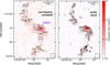 |
Fig. 2 Left: Combined ALMA 1.3 mm continuum map of I19074 with 26 cores overlaid (gray ellipses). The gray dashed contour marks the 2 σ1.3 mm boundary. Protostellar cores are marked as green stars. Right: ALMA-alone 1.3 mm continuum map with black contours ([3, 5, 10, 20, 40, 80, and 160] × σ1.3 mm, σ1.3 mm=0.08 mJy beam−1). Hierarchical structures Fn and Fs are bounded by the gray dashed contour at the 2 σ1.3 mm level. Blue plus marks the position of identified UC H II region by Lu et al. (2018). The synthesized beam and 0.5 pc scale bar are shown in right corners. |
3.1.2 Identification of dense cores
Cheng et al. (2024) compared the performance of two widely used core extraction algorithms, getsf (Men’shchikov 2021) and astrodendro (Rosolowsky et al. 2008), across the full sample of the INFANT survey. They found that getsf performs well only in identifying compact dense cores or fragments, whereas astrodendro is better suited for extracting additional extended and/or weak fragments that exhibit low intensity contrast against their background. To ensure a relatively robust fragmentation analysis of the I19074 region, we adopted the astrodendro algorithm to extract the dense fragments in this region. This method is well suited for identifying dense leaf-like structures (hereafter referred to as cores), which are the smallest structures without substructures under the terminology of the algorithm (Rosolowsky et al. 2008).
Following the parameter settings outlined in Cheng et al. (2024), we extracted a total of 27 cores from the ALMA-alone 1.3 mm continuum map: 26 cores along the S-shaped filament, plus additional one located away from the filament (not analyzed further). The number of the cores identified here is higher than that (i.e., 15 sources) reported by Cheng et al. (2024) using the getsf algorithm, which ensures a rather complete sample of cores for fragmentation analysis in this study. We note that the ALMA-alone data were used for core extraction rather than the combined 1.3 mm image. This choice was made by the fact that the ALMA-alone data already provide a sufficient maximum recoverable scale (12.4′′) to capture the bulk emission of compact sources, whereas the combined 1.3 mm image could include large-scale background emission, which acts as a contaminant on both core identification and flux measurement. The core parameters extracted by the algorithm are listed in Table 2, including the core name, coordinates, full width at half maximum (FWHM), position angle, effective radius, and integrated 1.3 mm flux. Further details regarding the extraction procedure can be found in Appendix B.
Figure 2 shows the spatial distribution of the extracted cores overlaid on the ALMA 1.3 mm continuum map. The 26 cores identified along the major S-shaped filament closely trace regions of compact dust emission, indicating the effectiveness of astrodendro for source extraction in the I19074 region. Among these cores, six can be classified as protostellar candidates following the criteria in Cheng et al. (2024) and Zhen et al. (2025) (see Fig. 2 and Table 2). In a nutshell, we searched for molecular outflows and/or warm gas tracers indicative of ongoing star formation. This was done using multiple molecular line transitions, including CO 2−1, SiO 5−4, as well as SO, H2 CO, and CH3 OH lines (see Cheng et al. 2024 and Zhen et al. (2025) for details). As a result, the Fs segment contains 6 prestellar and 3 protostellar cores, while the Fn segment hosts 14 prestellar and 3 protostellar cores (see Appendix C for details).
Parameters of dense cores.
3.2 Derived parameters of filamentary structures and cores
The masses of the density structures (i.e., filaments and cores) were derived using a graybody radiative transfer model under the optically thin approximation (Hildebrand 1983; Liu et al. 2021), expressed as
 (1)
In this equation, Sv represents the integrated 1.3 mm continuum flux of the density structures. For the filamentary structures, Sv was derived from the combined 1.3 mm continuum data (see Table 1), while for cores it was obtained from the ALMA-alone data (see Table 2). Here, d is the source distance, the gas-to-dust mass ratio, Rgd, is assumed to be 100, and the dust opacity, κv is taken as 0.899 cm2 g−1 at 1.3 mm (Ossenkopf & Henning 1994). We assumed that gas and dust are in equilibrium with each other, and thus Td can be approximated as the gas temperature. Tg. Here, we estimated Tg for the density structures in question from the NH3 rotational temperature map (see Fig. D, and Lu et al. 2018) by taking the mean value over the boundaries of each structure. This approach is appreciated since it has been suggested that Tg and the NH3 rotation temperature trace similar thermal states for molecular gas typically below ∼30 K (Lu et al. 2014). The resulting gas temperatures Tg are listed in Table 1 for filamentary structures and in Table 2 for cores.
(1)
In this equation, Sv represents the integrated 1.3 mm continuum flux of the density structures. For the filamentary structures, Sv was derived from the combined 1.3 mm continuum data (see Table 1), while for cores it was obtained from the ALMA-alone data (see Table 2). Here, d is the source distance, the gas-to-dust mass ratio, Rgd, is assumed to be 100, and the dust opacity, κv is taken as 0.899 cm2 g−1 at 1.3 mm (Ossenkopf & Henning 1994). We assumed that gas and dust are in equilibrium with each other, and thus Td can be approximated as the gas temperature. Tg. Here, we estimated Tg for the density structures in question from the NH3 rotational temperature map (see Fig. D, and Lu et al. 2018) by taking the mean value over the boundaries of each structure. This approach is appreciated since it has been suggested that Tg and the NH3 rotation temperature trace similar thermal states for molecular gas typically below ∼30 K (Lu et al. 2014). The resulting gas temperatures Tg are listed in Table 1 for filamentary structures and in Table 2 for cores.
To further investigate the nature of the cores, we calculated their mass surface densities, Σcore, as below:
 (2)
where Mcore is the core mass derived from Eq. (1), and Rcore is the core radius, equivalent to the geometric mean of the major and minor axes of the core’s FWHM size. The H2 number density of the cores, nH2, was then derived using the expression,
(2)
where Mcore is the core mass derived from Eq. (1), and Rcore is the core radius, equivalent to the geometric mean of the major and minor axes of the core’s FWHM size. The H2 number density of the cores, nH2, was then derived using the expression,
 (3)
where μH2 is the mean molecular weight per H2 molecule (adopted as 2.8, following Kauffmann et al. (2008)) and mH is the mass of a hydrogen atom.
(3)
where μH2 is the mean molecular weight per H2 molecule (adopted as 2.8, following Kauffmann et al. (2008)) and mH is the mass of a hydrogen atom.
The above derived parameters for the segment are presented in Table 1, while those for the individual cores are tabulated in Table 2. We note that these derivations carry uncertainties arising from several sources. The first is a 10% uncertainty in the kinematic distance. The second is a 5% uncertainty in the flux measurements from ALMA observations (see the ALMA Technical Handbook2). Additionally, the adopted values for the dust opacity, κν, and the gas-to-dust mass ratio, Rgd, could exhibit variability depending on the local cloud environment, ranging from diffuse to dense molecular gas (e.g., Martin et al. 2012; Roy et al. 2013; Webb et al. 2017). Here, we adopted uncertainties of 23% for Rgd and 28% for κν, in accordance with previous studies (e.g., Sanhueza et al. 2017; Xu et al. 2024; Shen et al. 2024). To account for the combined uncertainties, we performed a Monte Carlo simulation using 10 000 random samples, assuming a uniform distribution across the range of plausible values for each parameter. The resulting uncertainties for the final derived parameters (e.g., mass and number density) correspond to the 16th and 84th percentiles of the distribution, representing the lower and upper bounds, respectively.
As summarized in Table 1, the S-shaped filament, along with the Fs and Fn segments, have masses of approximately 913 M⊙, 248 M⊙, and 656 M⊙, respectively. From Table 2, the cores show a wide range of masses from 1.0 M⊙ to 22.9 M⊙ with a median value of 3.7 M⊙. Their mass surface densities span a range of [0.4, 4.1] g cm−2 with a median of 1.2 g cm−2, while their number densities fall between 1.2 × 10⁶ and 2.1 × 107 cm−3 with a median of 5.4 × 106 cm−3.
Another critical parameter for characterizing the cores is the virial parameter, αvir, which provides insight into their gravitational boundness. It is defined as:
 (4)
where σtot is the total velocity dispersion of the molecular gas (see below for details).
(4)
where σtot is the total velocity dispersion of the molecular gas (see below for details).
To estimate σtot for the molecular gas within the cores of the I19074 region, we relied on the kinematics observations of the NH3 line by Lu et al. (2014) rather than the H2 CO(32,2−22,1) and (32,1−22,0) transitions probed by the INFANT survey3. This choice was made due to the low detection rate of the H2 CO(32,2−..22,1) and H2 CO(32,1−22,0) lines across the I19074 region. We first deconvolved the observed core-averaged velocity dispersion of NH3(σobs, NH3) using the method described by Lu et al. (2018), expresssed as
 (5)
where 0.62 km s−1 is the channel spacing of the NH3 observations. Subsequently, the σtot parameter was calculated as:
(5)
where 0.62 km s−1 is the channel spacing of the NH3 observations. Subsequently, the σtot parameter was calculated as:
 (6)
where σnth is the non-thermal velocity dispersion, and
(6)
where σnth is the non-thermal velocity dispersion, and  is the thermal sound speed. Here, μp=2.33 is the mean molecular weight per free particle accounting for 90% hydrogen and 10% helium by number (e.g., Liu et al. 2019), while the molecular weight of NH3 is 17. In addition, the kinematic temperature, TNH3, is assumed to be the same as Tg (see above).
The resulting σtot of the cores span a range from 0.24 to 0.75 km s−1 (Table 2). Correspondingly, the virial parameters αvir range between 0.1 and 6.0. The gravitational boundness of the cores can be accordingly classified based on their virial parameters: systems with αvir ≤ 2 are considered (sub)virial and are gravitationally bound, making them prone to collapse; conversely, systems with αvir>2 are supervirial and require additional support, such as external pressures, to resist expansion (McKee & Holliman 1999; Kauffmann et al. 2013). In the I19074 region, the majority of the cores have αvir ≤ 2 within the uncertainties, and thus they are gravitationally bound toward the likely collapse. Only two cores (C4 and C14) exhibit αvir>2, which could be related to their protostellar nature with active star forming feedback (see Table 2).
3.3 Stability of filaments
The comparison between the observed line mass ( ) and the critical line mass (
 ) provides a useful diagnostic for assessing the gravitational stability of filaments. For an unmagnetized, isothermal filament, the theoretical critical line mass (Inutsuka & Miyama 1997; Wang et al. 2014) can be expressed as
 (7)
where G is the gravitational constant, and σeff represents the effective sound speed.
(7)
where G is the gravitational constant, and σeff represents the effective sound speed.
The σeff parameter corresponds to either the purely thermal contribution (cs) or a combination of thermal and turbulent motions (σtot). Based on the gas temperature of the filamentary structures, their thermal sound speeds yield critical line masses of ∼30 M⊙ pc−1 (see Table 1). To incorporate the effects of turbulence, we estimated the total velocity dispersion of the filamentary structures in a manner analogous to that used for core analysis in Eq. (6) of Sect. 3.2, utilizing NH3 observations. This approach results in σtot=0.41 km s−1 for the S-shaped filament, 0.36 km s−1 for the Fs segment, and 0.47 km s−1 for Fn. Correspondingly, the critical line masses accounting for turbulent motions were calculated to be ∼78 M⊙ pc−1 for the S-shaped filament, ∼60 M⊙ pc−1 for Fs, and ∼103 M⊙ pc−1 for Fn. These values are much lower than the observed line masses of the filamentary structures, which amount to 326 M⊙ pc−1 (S-shaped filament), 248 M⊙ pc−1 (Fs), and 364 M⊙ pc−1 (Fn). Accounting for projection angle of 45°, these values become 228 (S-shaped filament), 177 (Fs), and 262 M⊙ pc−1(Fn). This result indicates that all three filamentary structures are gravitationally bound and are undergoing collapse to form smaller and denser substructures, which is consistent with the presence of dense cores aligned along the filamentary structures.
3.4 Hierarchical fragmentation analysis of the filaments
3.4.1 Filaments fragmentation
As shown in Fig. 2, the observed separations between dense cores along the S-shaped filament axis do not show a clear periodicity. Instead, four distinct groups of cores appear to be regularly distributed along the same axis (see Fig. 3). We associated these four groups with the corresponding clumps (clumps 1-4; see Fig. 3). They were defined based on the central positions of compact sources revealed from SMA 1.3 mm dust continuum emission (see Fig. 1, Lu et al. 2018), as well as a detection threshold of 9 σ1.2 mm in MAMBO 1.2 mm dust continuum emission (Fig. 3). While the actual boundaries of these clumps are not rigorously defined here, the current approximate delineation was sufficient for the purposes of our subsequent analysis. The observed parameters of these clumps were measured from MAMBO 1.2 mm continuum emission, including the coordinates, FWHM size, position angle, effective radius, and integrated flux. Likewise, the temperature of the clumps was extracted from the NH3 rotational temperature map. The mass and number density of the clumps were derived following Eqs. (1) and (3), but with the core radii replaced by the clump radii. All these parameters are listed in Table 3.
In the following, we analyze the S-shaped filament fragmentation into two parts, one for Fn and the other for, since the two filamentary segments present different fragmentation processes (see Sect. 4.2). In a nutshell, we find that Fn could first fragment through the filamentary mode into three regularly spaced clumps (i.e., clumps 2-4), followed by clump fragmentation into individual dense cores. The average separation between the clumps were measured to be λobs ∼0.7 pc (see Fig. 3), which corresponds to a deprojected spacing of  pc accounting for an inclination angle of 45° with respect to the the plane of the sky (see Sect. 3.1.1). In contrast, Fs could fragment through the filamentary end-dominated mode as proposed in previous studies (e.g., Clarke & Whitworth 2015) since this filament has only a single compact fragment (i.e., clump 1) located specifically at the southern end of Fs.
To investigate the fragmentation mechanism within the northern Fn segment, we adopted the shocked-gas shell fragmentation model proposed by Whitworth et al. (1994), instead of the standard semi-analytic cylinder fragmentation models (e.g., Inutsuka & Miyama 1992) widely used for such analysis. The shocked shell fragmentation model describes formation of density structures in dynamically perturbed environments, where shocks compress the gas into dense layers/filaments that are prone to fragmentation. In contrast, the cylinder fragmentation model accounts for gravitational instabilities within pre-existing filaments embedded in non or relatively weakly shocked gas environments. Indeed, the spatial association between Fn and the adjacent H II region suggests that the Fn segment could represent a gas shell shocked by the expansion of ionized gas.
Following Whitworth et al. (1994), several key physical properties of the fragments/clumps produced via shell fragmentation can be estimated using simplified analytical expressions. These include the fragmentation timescale (tfrag), the characteristic mass of the fragments (Mfrag), and their typical separation (Sfrag). The relevant expressions particularly for the case of a shocked gas shell surrounding an H II region being thermally expanding (Whitworth et al. 1994) are as follows:
 (8)
(8)
 (9)
(9)
 (10)
where a.2 is the velocity dispersion of Fn(0.47 km s−1) within the shell in units of 0.2 km s−1; Ṅ49 denotes the ionizing photon flux in units of 1049 ph s−1; and n3 represents the initial atomic number density of the gas in units of 103 cm−3. For the Fn segment, we estimated a.2 ∼2.30 based on the effective velocity dispersion measured within this segment (see Table 1). The ionizing photon flux and initial gas density are adopted as Ṅ49=0.16 and n3=22.0, respectively (see Appendix E for detailed derivations and assumptions underlying these estimates).
(10)
where a.2 is the velocity dispersion of Fn(0.47 km s−1) within the shell in units of 0.2 km s−1; Ṅ49 denotes the ionizing photon flux in units of 1049 ph s−1; and n3 represents the initial atomic number density of the gas in units of 103 cm−3. For the Fn segment, we estimated a.2 ∼2.30 based on the effective velocity dispersion measured within this segment (see Table 1). The ionizing photon flux and initial gas density are adopted as Ṅ49=0.16 and n3=22.0, respectively (see Appendix E for detailed derivations and assumptions underlying these estimates).
The predicted fragment mass from the model is 149 M⊙, which is roughly consistent with the observed masses of all clumps except for clump 2 (see in Table 3). The discrepancy emerging for clump 2 likely stems from the assumption in the theoretical model that the expanding H II region propagates into a uniform medium, whereas in reality, the gas distribution is more complex and inhomogeneous. In addition, the above calculations yield a fragmentation timescale of tfrag ∼0.8 Myr, which is comparable to the dynamical timescale of the associated expanding H II region (tdyn=0.7 Myr; see Appendix E for detailed calculations). This indicates that the Fn shell+filament has sufficient time to undergo fragmentation during the dynamical expansion phase of the H II region. The predicted fragment separation of 1 pc agrees reasonably well with the observed separation of  ∼1 pc between the clumps. This consistency supports the scenario in which the Fn segment undergoes fragmentation into clumps via the shell fragmentation mechanism.
We also explored the fragmentation mechanism of the Fn segment using the “sausage” model, a canonical example of cylinder fragmentation models. The central premise of the “sausage” model is that a self-gravitating, isothermal gas cylinder can fragment into dense fragments with quasi-periodic separations (e.g., Chandrasekhar & Fermi 1953; Nagasawa 1987). These periodic separations correspond to the critical wavelength (λcrit), at which the gravitational instability grows most rapidly. Following Jackson et al. (2010); Lu et al. (2018), we adopted the expression for λcrit for an assumed infinite isothermal gas cylinder λcrit=22 ceff(4 π G ρc)−0.5. Here, the effective sound speed ceff is taken as the total velocity dispersion of the Fn segment, estimated to be ∼0.47 km s−1 (see Table 1). The central gas density of the filament is approximated by the average density of the dense cores, ρc ≈ 3.5 × 10⁻¹⁷ g cm−3 (equivalent to 7.5 × 106 cm−3). It is worth noting that the density, ρc, used in this analysis corresponds to the centermost density of the filament, rather than the average component, and we therefore took the core’s density as a first order of approximation. Using these parameters, the calculated λcrit value is 0.06 pc, which is substantially lower than the observed separation between clumps ( ). This significant discrepancy further supports the conclusion that the shocked-gas shell fragmentation model provides a more appropriate framework for explaining the fragmentation of the Fn segment into clumps, as compared to the standard cylinder fragmentation model.
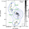 |
Fig. 3 Spatial distribution of dense cores in I19074. The background shows ALMA 1.3 mm continuum emission. Blue dots mark core locations and the yellow solid line denotes the minimum path connecting these elements, given by the MST algorithm. The green dashed ellipses indicate clumps. The blue dashed contours are at [9, 15, 21, 27, and 33]× σ1.2 mm. The synthetic beam of 0.60′′ × 0.58′′ for ALMA observations and the scale bar of 0.5 pc are shown in right corners. |
Parameters of clumps.
3.4.2 Clump fragmentation
To investigate the fragmentation of clumps into dense cores, we considered a spherical, Jeans-like fragmentation mode. This theoretical framework is characterized by the critical Jeans length and critical Jeans mass. Comparing both theoretical predictions with observational measurements can offer insights onto the physical processes driving core formation within clumps. However, as noted by Beuther et al. (2018), observational mass estimates are subject to significant uncertainties, typically on the order of a factor of ∼2 (see Sect. 3.2). As a result, the core separation is adopted here as a more robust proxy for assessing the fragmentation properties within clumps.
We employed the minimum-spanning tree (MST) method, as described by Barrow et al. (1985) and Dib & Henning (2019), to determine the shortest projected separations between cores within each clump (see Fig. 3). This analysis yields observed core separations of 0.11−0.13 pc across all clumps, corresponding to de-projected spacings of 0.16−0.18 pc (see Table 4) accounting for a 45° inclination angle. Theoretically, the critical Jeans length λJ for a clump is given by
 (11)
where ceff is the effective speed of sound within the clump and ρeff is the average density of the clump.
(11)
where ceff is the effective speed of sound within the clump and ρeff is the average density of the clump.
If thermal motions alone govern the fragmentation process, ceff corresponds to the thermal speed of sound. For the clumps in our sample, with temperatures ranging from 17 to 20 K (see Table 3), ceff ≈ 0.26 km s−1. Using the derived gas densities of 8.3 × 10⁻²⁰ g cm−3 for clump 1, 8.0 × 10⁻²⁰ g cm−3 for clump 2, 1.3 × 10⁻¹⁹ g cm−3 for clump 3, and 5.2 × 10⁻²⁰ g cm−3 for clump 4 (corresponding to 1.8 × 10⁴, 1.7 × 10⁴, 2.8 × 10⁴, and 1.1 × 104 cm−3, respectively, see Table 3), λJ was calculated to be ∼0.19 pc for all clumps (see Table 4). This value is comparable to the average deprojected core separation (i.e., ∼0.17 pc) over all the clumps (see Table 4).
Estimated Jeans parameters for clumps.
4 Discussion
4.1 Link between S-shaped filament formation and the expanding HII region
As analyzed in Sect. 3.1.1, the whole S-shaped filament consists of the northern Fn and southern Fs segments (see Fig. 2). In particular, the Fn filamentary segment is associated with the classical H II region. This spatial association indicates a physical interaction between them driven by the radiative and mechanical feedback from ionized gas within the H II region.
This interaction has been envisioned in the “collect and collapse” (C&C) model proposed by Elmegreen & Lada (1977). In this model, ionizing radiation from massive stars within an H II region generates an ionization front (IF), which expands into the surrounding molecular cloud. The supersonic expansion of the H II region drives a shock front (SF) ahead of the IF. Gas compressed between the IF and the SF accumulates into a new dense gas shell/filament. Over time, this filament becomes gravitationally unstable, fragments into clumps through the shocked fragmentation mode (see Sect. 3.4.1, Whitworth et al. 1994), and eventually forms dense cores where star formation ensues. The C&C model could in part provides a plausible framework for understanding formation and evolution of the northern Fn segment under the influence of an expanding H II region. This aligns with the similarity between tfrag for Fn and tdyn for the expanding H II region. This timescale relation suggests that the expanding H II region has had sufficient time to influence formation and evolution of the Fn segment.
Alternatively, the filamentary Fn segment could be in part pre-existing prior to the expansion of the associated H II region. This interpretation is supported by the strong spatial and kinematic connection between the Fn and Fs segments. Spatially, both segments converge toward central clump 2, while kinematically they exhibit nearly identical systemic velocities, with only a slight offset of ∼1.5 km s−1 (see the H2 CO 30,3−20,2 velocity map in Appendix A). These tight couplings suggest that Fn and Fs likely originated from the same large-scale filamentary structure within a somehow quiescent molecular cloud environment, which is in good agreement with the Fs association with an IRdark signature in 8 μm emission typical of a relatively quiescent environment.
Therefore, we propose the following hybrid scenario for Fn formation that incorporates both the swept-up compression of a pre-existing filamentary structure and the simultaneous accumulation of fresh gas within the shocked layer. In other words, both Fn and Fs segments could initially form as part of a single, linear filament within a quiescent molecular cloud. Subsequently, high-mass star formation initiated early on at a position in the Fn segment, but located within its western side. Ionizing radiation from high-mass star(s) then triggered the expansion of the associated H II region, which swept up and compressed the northern part of the pre-existing filament toward the east. This process displaced the northern part spatially and kinematically from the southern one, leading to the presence of the Fn and Fs segments. Furthermore, the Fn segment was reshaped into an arc-like morphology due to the swept-up by the H II region, while the Fs remained largely unaffected due to its location away from the H II region. As a result, the swept-up process finally rendered the primordial linear filament to be an S-shaped structure. During the swept-up phase, the Fn segment grew in extra mass by the accumulation of fresh gas between the SF and IF, which is consistent with a greater observed line mass for Fn compared to Fs. This accumulation could be consistent with the observational signature showing the apparent merging of two small-scale gas flow branches, exhibiting slightly different velocities (<1 km s−1), with the main body of the Fn segment, as observed in the H2 CO 30,3−20,2 velocity (moment 1) map (see Appendix A). In the context of the swept-up process, the observed velocity offset of ∼1.5 km s−1 between Fn and Fs could be interpreted as the expansion velocity of the H II region. This value is consistent with the typical expansion velocities (a few km s−1) reported for other expanding H II regions (Liu et al. 2016; Pabst et al. 2020; Bonne et al. 2022).
Accordingly, the observed kinetic energy of the Fn segment,  , can be estimated to be ∼1.5 × 1046 erg. This value is consistent with the predicted kinetic energy of ∼4.9 × 1046 erg of the expanding molecular shell resulting from energy transfer via the Lyman continuum within the H II region (see Appendix E for details). This consistency indicates that the ionizing radiation emitted by the massive star(s) powering the H II region in 119074 provides sufficient energy to drive the expansion of the surrounding molecular gas shell. This, in turn, leads to the eastward displacement of the Fn filament, resulting in its characteristic bent morphology.
4.2 Hierarchical fragmentation in the S-shaped filament
Dense cores are closely associated with the S-shaped filament (see Fig. 2). This leads to a core formation scenario in which the supercritical S-shaped filament (with  , see Table 1) fragments longitudinally into individual cores or groups of cores. As mentioned in Sect. 3.4.1, the fragmentation of the entire S-shaped filament can be divided into two distinct segments: one corresponding to the northern Fn segment and the other to the southern Fs segment.
As for the Fs segment, its fragmentation could be explained by the filamentary end-dominated collapse model. This model was proposed through theoretical investigations of the evolution of a quiescent, finite-length filament and is characterized by an enhanced global collapse occurring preferentially at either end of the filamentary structure. The enhancement in collapse at the filament ends arises due to the increasing importance of nonlinear terms in the gravitational acceleration (Bastien 1983). Within this framework, the resulting fragmentation mechanism is interpreted as edge fragmentation (Hacar et al. 2023). Observationally, both Fs and its associated dense cores are located within an IR-dark environment and a group of cores within clump 1 are predominantly situated toward the southern end of the Fs segment. These observational features suggest that core formation in Fs would result from edge fragmentation driven by gravitational instability at the filament’s end.
Regarding the Fn segment, dense cores appear to have formed in the interior of the filament, in contrast to those in Fs residing at the filament southern edge. This difference suggests that Fn follows a different fragmentation pathway than Fs. In Sect. 3.4.1, we explain that we have not found that the observed separations between clumps along Fn align with the predicted distribution of periodic chains of cores via standard semi-analytic cylinder fragmentation models (e.g., Inutsuka & Miyama 1992). This inconsistency between observations and simple theoretical predictions could arise because actual molecular filaments are not isolated and hydrostatically equilibrium structures (Clarke et al. 2017; Pineda et al. 2023). Through simulations of molecular gas filaments undergoing dynamical accretion from a turbulent environment, Clarke et al. (2017) demonstrated that fragmentation occurs in a hierarchical fashion, wherein large-scale filamentary fragmentation modes develop first, followed by smaller-scale, spherical Jeans-like fragmentation at later stages. This hierarchical fragmentation paradigm provides a plausible explanation for the scale-dependent fragmentation observed in Fn. In this scenario, the Fn segment initially fragments on a large scale into three regularly spaced clumps; namely, clump 2, clump 3, and clump 4, with a typical deprojected separation of ∼1 pc between them. Subsequently, each clump undergoes smaller-scale, spherical fragmentation, producing randomly distributed dense cores with a typical deprojected separation of ∼0.17 pc. The stochastic distribution of cores within the clumps likely contributes to the apparent lack of periodicity in the overall core distribution along the filament. The similar hierarchical fragmentation process has been identified in a few other filaments, such as the Orion integral-shaped filament (Orion-ISF), through high-resolution interferometric mosaic observations (Takahashi et al. 2013; Teixeira et al. 2016; Kainulainen et al. 2013, 2017; Shimajiri et al. 2019; Zhen et al. 2025).
What are the mechanisms for the scale-dependent hierarchical fragmentation processes? Analysis presented in Sect. 3.4.1 indicates that the associated expanding H II region does have sufficient time to regulate the formation and evolution of the Fn segment due to tfrag ≤ tdyn. In addition to the timescale relation, the observed separations between clumps in Fn are consistent with the characteristic spacing predicted by the C&C model. This consistency supports the interpretation that the fragmentation of the Fn segment into clumps proceeds via the shocked shell fragmentation mechanism due to gravitational instability, as described within the C&C framework (see Sect. 4.1).
Regarding the fragmentation mechanism within individual clumps, we do not find that the clumps in both Fn and Fs show any difference. In both cases, the observed core separations within clumps are in agreement with the predictions of thermal Jeans fragmentation in the absence of significant external support (see Sect. 3.4.2). This agreement suggests that the internal fragmentation of clumps is governed primarily by thermal processes.
4.3 High-mass star formation scenario in the S-shaped filament
From a theoretical perspective, the competing models of high-mass star formation can be broadly divided into two primary categories: the “core-fed accretion” paradigm (e.g., the turbulent core accretion model, McKee & Tan 2003) and the “clumpfed accretion” scenario (e.g., the competitive accretion model, Bonnell et al. 2001, 2004). In the core-fed accretion models, high-mass candidate prestellar cores can resist gravitational collapse and fragmentation due to the presence of strong turbulence and/or magnetic fields that provide support against further subdivision. Conversely, the clump-fed models suggest that high-mass stars form from initially Jeans-unstable fragments within a massive molecular clump, with these fragments subsequently gaining mass through ongoing gas accretion while competing gravitationally within the tidal environment of the parent clump. The detection (or absence) of high-mass candidate prestellar cores serves as a critical observational test to distinguish between these two competing formation pathways.
In the I19074 region, 92% of the 26 identified dense cores exhibit virial parameters of αvir ≤ 2 within the uncertainties (see Table 2), indicating that they are gravitationally bound and likely undergoing collapse toward star formation. Furthermore, with the exception of eight cores (C2, C4, C8, C12, C17, C19, C23, and C24), all cores in 119074 have mass surface densities of Σcore ≥ 1 g cm−2, exceeding both the theoretical threshold for high-mass star formation proposed by Krumholz & McKee (2008) and the empirical limit of 0.05 g cm−2 derived from observations by Urquhart et al. (2014). These cores could therefore be sufficiently dense to potentially form high-mass stars. This is particularly likely for those with relatively high gas masses (e.g., C6, C7, C10, C15, and C18, each with Mcore>8 M⊙).
Based on the lack of detectable star-formation signatures, 23 of 26 dense cores were tentatively classified as prestellar candidates (see Sect. 3). Among these, the two most massive prestellar candidates (cores C10 and C15) have masses of approximately 16 M⊙, approaching the critical mass threshold for high-mass starless cores as defined by the ALMA-IMF survey team under the assumption of a relatively high core-to-star formation efficiency of 50% (e.g., Valeille-Manet et al. 2023; Nony et al. 2023; Valeille-Manet et al. 2025). However, with sizes of about 8000 AU, these cores may harbor smaller-scale, unresolved dense fragments resulting from further fragmentation, which remains undetected at our current angular resolution. This implies that true high-mass candidate prestellar cores are likely rare in I19074 and the majority (if not all) of the prestellar population consists of low-mass cores. This conclusion is in agreement with the finding from large-scale surveys, such as the ASHES project (Sanhueza et al. 2019). The apparent scarcity of high-mass candidate prestellar cores in I19074 favors clump-fed accretion-type models over core-fed accretion-type models for high-mass star formation.
As discussed in Sect. 3.4, the filament-to-clump fragmentation processes in Fn and Fs are governed by distinct driving mechanisms: the shocked shell fragmentation mechanism in the framework of the C&C (e.g., Ginsburg et al. 2015; Chen et al. 2022; Saha et al. 2024) model for Fn, and the edge-fragmentation mechanism in the framework of the end-dominated collapse model for Fs. Both fragmentation driving pathways could promote necessary conditions favorable for high-mass star formation. In the C&C framework, a gravitationally unstable, shocked gas shell forms as a result of efficient mass accumulation due to strong compression by an expanding H II region around massive stars. This shocked shell is therefore prone to fragmentation into massive, well-separated clumps that are expected to produce a high fraction of high-mass stars (Whitworth et al. 1994). In contrast, the end-dominated collapse model posits that gravitational focusing becomes increasingly nonlinear toward the filament ends, causing them to accelerate more rapidly than the filament interiors. This leads to enhanced gas inflow and density enhancement at the filament ends, favoring formation of dense, massive fragments near the ends (Clarke & Whitworth 2015). In the I19074 region, clump 1 in Fs and clump 2 in Fn (i.e., products of edge-fragmentation and shocked shell fragmentation, respectively) exhibit substantial masses within relatively compact radii: ∼240 M⊙ within 0.4 pc for clump 1 and ∼620 M⊙ within 0.5 pc for clump 2. These mass reservoirs lie far above the mass-radius threshold of 1 g/cm2 for high-mass star formation (see above, Krumholz & McKee 2008). This finds further support from the observed fact that each clump hosts one of the two most massive cores identified in the region, with masses of ∼16 M⊙. In particular, clump 2 contains an embedded UCH II region, a strong indicator of ongoing high-mass star formation. Taken together, these findings suggest that both the shocked shell fragmentation mechanism in Fn and the edge-fragmentation mechanism in Fs could be effective pathways for producing massive, starforming clumps. We therefore propose that both mechanisms contribute to high-mass star formation within their respective filaments through a dynamical clump-fed accretion process.
5 Summary
We present new 1.3 mm continuum observations of the S-shaped molecular filament I19074 with ongoing high-mass star formation, obtained at an angular resolution of ∼0.60′′(∼6000 AU) as part of the ALMA-INFANT survey. We investigated the physical processes linking filament formation, fragmentation, and the dynamical scenario of high-mass star formation within the 119074 region. The major findings are summarized as follows.
The S-shaped filament comprises two distinct components: a southern segment (Fs) and a northern one (Fn). These segments are spatially and kinematically connected, with a modest velocity offset of ∼1.5 km s−1. The Fn segment is associated with an IR-bubble +H II region bright in 8 μm emission, whereas Fs appears relatively IR-dark in same emission. Accounting for projection effects, we derived the following properties from ALMA 1.3 mm dust continuum emission: the total length of the S-shaped filament is ∼2.8 pc, with Fs and Fn measuring ∼1.8 pc and ∼1.0 pc, respectively. Their corresponding masses are 910 M⊙, 250 M⊙, and 660 M⊙, and their line masses are 330 M⊙ pc−1, 250 M⊙ pc−1, and 360 M⊙ pc−1, respectively. All the line masses significantly exceed the critical value required to overcome the turbulence support, indicating that these filamentary structures could be supercritical and, thus, gravitationally bound.
The association between the northern Fn segment and the classical H II region, along with the strongly spatial and kinematic connection between Fn and Fs, suggests that the expansion of the H II region has swept up and reshaped the primordial linear filament into its current S-shaped morphology. In this scenario, Fn was compressed into an arc-like structure due to interaction with the expanding H II region, while Fs retained a relatively linear morphology due to its location farther from the ionized region. Accordingly, a hybrid formation mechanism is proposed for Fn, involving both the compression of a pre-existing filament by the expanding H II region and the simultaneous accumulation of fresh gas within the shocked filament. This interpretation is supported by the comparable timescales of tfrag for Fn (∼0.8 Myr) and tdyn of the expanding H II region, indicating that the H II region had sufficient time to influence the formation and even evolution of Fn.
A total of 26 dense cores were identified along the Sshaped filament from ALMA 1.3 mm dust continuum emission. These cores exhibit a broad range of masses from 1.0 M⊙ to 22.9 M⊙ with a median value of 3.7 M⊙. Their mass surface densities span [0.4, 4.1] g cm−2, with a median value of 1.2 g cm−2, and their number densities range from 1.2 × 106 cm−3 to 2.1 × 107 cm−3, with a median of 5.4 × 106 cm−3. Approximately 92% of the cores have virial parameters αvir ≤ 2 within uncertainties, indicating that they are gravitationally bound and likely undergoing collapse toward star formation.
The projected separations between dense cores along the filament axis do not exhibit clear periodicity. Instead, four distinct groups of cores are somehow regularly distributed along the filament, which we associate with four corresponding clumps: clump 1 through clump 4. These clumps have masses ranging from 110 M⊙ to 620 M⊙, with radii between 0.24 pc and 0.5 pc. Clump 1 is located at the southern end of Fs, while clumps 2-4 are regularly spaced along Fn.
The absence of periodicity in the spatial distribution of the 26 filament-hosted cores, combined with the distinct spatial arrangement of the four clumps along Fs and Fn, suggests that the fragmentation of the S-shaped filament can be divided into two distinct segments. In Fs, the cores within clump 1 are predominantly located at the southern end of the segment, consistent with the edge fragmentation mechanism driven by gravitational instability. This behavior aligns with the filamentary end-dominated collapse model, in which a finite-length filament evolves via enhanced global collapse preferentially occurring at its ends. In contrast, the fragmentation of Fn appears to proceed in a hierarchical manner. Large-scale filamentary fragmentation initially produces three regularly spaced clumps (clump 2, clump 3, and clump 4) with a typical deprojected separation of ∼1 pc. Subsequent smaller-scale, Jeans-like fragmentation within each clump generates randomly distributed dense cores with a typical separation of ∼0.17 pc. The stochastic distribution of cores within the clumps could lead to the observed lack of periodicity along the filament. In addition to the comparable timescales between tfrag ∼tdyn, the observed separations between clumps in Fn are consistent with the characteristic spacing predicted by the C&C model. These consistencies support that fragmentation of the Fn segment into clumps proceeds via the shocked shell fragmentation mechanism due to gravitational instability as described within the C&C framework.
Within individual clumps in both Fn and Fs, the observed separations between dense cores are consistent with predictions from thermal Jeans fragmentation in the absence of significant non-thermal support. This indicates that internal fragmentation within the clumps in the I19074 region is primarily governed by thermal processes.
With the exception of eight cores (C2, C4, C8, C12, C17, C19, C23, and C24), all cores in the I19074 region exhibit mass surface densities Σcore ≥ 1 g cm−2, suggesting sufficient density to potentially form high-mass stars. We did not identify robust high-mass prestellar candidates. This result favors dynamical clump-fed accretion models over more static core-fed accretion scenarios for high-mass star formation in the I19074 region.
To conclude, our findings provide a coherent picture of the physical processes connecting filament formation, fragmentation, and a dynamical scenario of high-mass star formation in the I19074 region. The S-shaped filament likely formed through the interaction with an expanding H II region, with the shockedshell fragmentation mechanism in Fn and edge fragmentation in Fs serving as effective pathways for producing massive, starforming clumps. Both mechanisms contribute to high-mass star formation via a dynamical clump-fed accretion process within their respective filamentary segments.
Acknowledgements
This work is supported by the National Key R&D Program of China (No. 2022YFA1603101) and the National Natural Science Foundation of China (NSFC) through grant Nos. 12273090 and 12322305. H.-L.L. is supported by Yunnan Fundamental Research Project (grant No. 202301AT070118, 202401AS070121), and by Xingdian Talent Support Plan-Youth Project. X.L. is supported by the Strategic Priority Research Program of the Chinese Academy of Sciences (CAS) Grant No. XDB0800300, the Natural Science Foundation of Shanghai (No. 23ZR1482100) and the CAS “Light of West China” Program No. xbzg-zdsys-202212. X.L. acknowledges support from the Strategic Priority Research Program of the Chinese Academy of Sciences (CAS) Grant No. XDB0800303. R.G.M is support by DGAPA UNAM PAPIIT project IN105225. P.S was partially supported by a Grant-in-Aid for Scientific Research (KAKENHI Number JP22H01271 and JP23H01221) of JSPS.
References
- Álvarez-Gutiérrez, R. H., Stutz, A. M., Sandoval-Garrido, N., et al. 2024, A&A, 689, A74 [NASA ADS] [CrossRef] [EDP Sciences] [Google Scholar]
- Anderson, L. D., Bania, T. M., Balser, D. S., et al. 2014, ApJS, 212, 1 [Google Scholar]
- André, P., Men’shchikov, A., Bontemps, S., et al. 2010, A&A, 518, L102 [NASA ADS] [CrossRef] [EDP Sciences] [Google Scholar]
- André, P., Di Francesco, J., Ward-Thompson, D., et al. 2014, in Protostars and Planets VI, eds. H. Beuther, R. S. Klessen, C. P. Dullemond, & T. Henning (Tucson: University Of Arizona Press), 27 [Google Scholar]
- André, P., Arzoumanian, D., Könyves, V., Shimajiri, Y., & Palmeirim, P., 2019, A&A, 629, L4 [Google Scholar]
- Arzoumanian, D., André, P., Könyves, V., et al. 2019, A&A, 621, A42 [NASA ADS] [CrossRef] [EDP Sciences] [Google Scholar]
- Barrow, J. D., Bhavsar, S. P., & Sonoda, D. H., 1985, MNRAS, 216, 17 [NASA ADS] [CrossRef] [Google Scholar]
- Bastien, P., 1983, A&A, 119, 109 [NASA ADS] [Google Scholar]
- Benjamin, R. A., Churchwell, E., Babler, B. L., et al. 2003, PASP, 115, 953 [Google Scholar]
- Beuther, H., Schilke, P., Menten, K. M., et al. 2002, ApJ, 566, 945 [Google Scholar]
- Beuther, H., Mottram, J. C., Ahmadi, A., et al. 2018, A&A, 617, A100 [NASA ADS] [CrossRef] [EDP Sciences] [Google Scholar]
- Bonne, L., Schneider, N., García, P., et al. 2022, ApJ, 935, 171 [NASA ADS] [CrossRef] [Google Scholar]
- Bonnell, I. A., Bate, M. R., Clarke, C. J., & Pringle, J. E., 2001, MNRAS, 323, 785 [Google Scholar]
- Bonnell, I. A., Vine, S. G., & Bate, M. R., 2004, MNRAS, 349, 735 [Google Scholar]
- CASA Team, Bean, B., Bhatnagar, S., et al. 2022, PASP, 134, 114501 [NASA ADS] [CrossRef] [Google Scholar]
- Chandrasekhar, S., & Fermi, E., 1953, ApJ, 118, 116 [Google Scholar]
- Chen, H.-R. V., Zhang, Q., Wright, M. C. H., et al. 2019, ApJ, 875, 24 [Google Scholar]
- Chen, Z., Sefako, R., Yang, Y., et al. 2022, Res. Astron. Astrophys., 22, 075017 [Google Scholar]
- Cheng, Y., Lu, X., Sanhueza, P., et al. 2024, ApJ, 967, 56 [Google Scholar]
- Clarke, S. D., & Whitworth, A. P., 2015, MNRAS, 449, 1819 [NASA ADS] [CrossRef] [Google Scholar]
- Clarke, S. D., Whitworth, A. P., Duarte-Cabral, A., & Hubber, D. A., 2017, MNRAS, 468, 2489 [Google Scholar]
- Dib, S., & Henning, T., 2019, A&A, 629, A135 [NASA ADS] [CrossRef] [EDP Sciences] [Google Scholar]
- Dyson, J. E., & Williams, D. A., 1980, Nature, 287, 373 [Google Scholar]
- Elmegreen, B. G., & Lada, C. J., 1977, ApJ, 214, 725 [Google Scholar]
- Federrath, C., Rathborne, J. M., Longmore, S. N., et al. 2016, ApJ, 832, 143 [NASA ADS] [CrossRef] [Google Scholar]
- Galván-Madrid, R., Zhang, Q., Keto, E., et al. 2010, ApJ, 725, 17 [Google Scholar]
- Ginsburg, A., Bally, J., Battersby, C., et al. 2015, A&A, 573, A106 [NASA ADS] [CrossRef] [EDP Sciences] [Google Scholar]
- Gómez, G. C., & Vázquez-Semadeni, E., 2014, ApJ, 791, 124 [Google Scholar]
- Hacar, A., Clark, S. E., Heitsch, F., et al. 2023, ASP Conf. Ser., 534, 153 [NASA ADS] [Google Scholar]
- He, Y.-X., Liu, H.-L., Tang, X.-D.,, et al. 2023, ApJ, 957, 61 [NASA ADS] [CrossRef] [Google Scholar]
- Hildebrand, R. H., 1983, QJRAS, 24, 267 [NASA ADS] [Google Scholar]
- Inutsuka, S.-I., & Miyama, S. M., 1992, ApJ, 388, 392 [CrossRef] [Google Scholar]
- Inutsuka, S.-i., & Miyama, S. M., 1997, ApJ, 480, 681 [NASA ADS] [CrossRef] [Google Scholar]
- Jackson, J. M., Finn, S. C., Chambers, E. T., Rathborne, J. M., & Simon, R., 2010, ApJ, 719, L185 [Google Scholar]
- Jayasinghe, T., Dixon, D., Povich, M. S., et al. 2019, MNRAS, 488, 1141 [NASA ADS] [CrossRef] [Google Scholar]
- Kainulainen, J., Ragan, S. E., Henning, T., & Stutz, A., 2013, A&A, 557, A120 [NASA ADS] [CrossRef] [EDP Sciences] [Google Scholar]
- Kainulainen, J., Stutz, A. M., Stanke, T., et al. 2017, A&A, 600, A141 [NASA ADS] [CrossRef] [EDP Sciences] [Google Scholar]
- Kauffmann, J., Bertoldi, F., Bourke, T. L., Evans, II, N. J., & Lee, C. W. 2008, A&A, 487, 993 [NASA ADS] [CrossRef] [EDP Sciences] [Google Scholar]
- Kauffmann, J., Pillai, T., & Goldsmith, P. F., 2013, ApJ, 779, 185 [NASA ADS] [CrossRef] [Google Scholar]
- Kirk, H., Klassen, M., Pudritz, R., & Pillsworth, S., 2015, ApJ, 802, 75 [NASA ADS] [CrossRef] [Google Scholar]
- Könyves, V., André, P., Arzoumanian, D., et al. 2020, A&A, 635, A34 [Google Scholar]
- Krumholz, M. R., & McKee, C. F., 2008, Nature, 451, 1082 [Google Scholar]
- Kumar, M. S. N., Palmeirim, P., Arzoumanian, D., & Inutsuka, S. I., 2020, A&A, 642, A87 [EDP Sciences] [Google Scholar]
- Kurtz, S., Churchwell, E., & Wood, D. O. S., 1994, ApJS, 91, 659 [Google Scholar]
- Kwan, J., 1997, ApJ, 489, 284 [Google Scholar]
- Lasker, B. M., 1967, ApJ, 149, 23 [Google Scholar]
- Li, S., Sanhueza, P., Zhang, Q., et al. 2020, ApJ, 903, 119 [Google Scholar]
- Li, S., Zhang, Q., Pillai, T., et al. 2019, ApJ, 886, 130 [Google Scholar]
- Liu, H. B., Jiménez-Serra, I., Ho, P. T. P., et al. 2012a, ApJ, 756, 10 [NASA ADS] [CrossRef] [Google Scholar]
- Liu, H. B., Quintana-Lacaci, G., Wang, K., et al. 2012b, ApJ, 745, 61 [NASA ADS] [CrossRef] [Google Scholar]
- Liu, H. B., Ho, P. T. P., Wright, M. C. H., et al. 2013, ApJ, 770, 44 [NASA ADS] [CrossRef] [Google Scholar]
- Liu, H.-L., Wu, Y., Li, J., et al. 2015, ApJ, 798, 30 [Google Scholar]
- Liu, H.-L., Li, J.-Z., Wu, Y., et al. 2016, ApJ, 818, 95 [Google Scholar]
- Liu, H.-L., Stutz, A., & Yuan, J.-H., 2018, MNRAS, 478, 2119 [NASA ADS] [CrossRef] [Google Scholar]
- Liu, H.-L., Stutz, A., & Yuan, J.-H., 2019, MNRAS, 487, 1259 [Google Scholar]
- Liu, H.-L., Liu, T., Evans, II, N. J., et al. 2021, MNRAS, 505, 2801 [NASA ADS] [CrossRef] [Google Scholar]
- Liu, H.-L., Tej, A., Liu, T., et al. 2022a, MNRAS, 511, 4480 [NASA ADS] [CrossRef] [Google Scholar]
- Liu, H.-L., Tej, A., Liu, T., et al. 2022b, MNRAS, 510, 5009 [NASA ADS] [CrossRef] [Google Scholar]
- Liu, H.-L., Tej, A., Liu, T., et al. 2023, MNRAS, 522, 3719 [NASA ADS] [CrossRef] [Google Scholar]
- Liu, X., Liu, T., Li, P.-S.,, et al. 2025, Nat. Astron., 9, 1366 [Google Scholar]
- Longmore, S. N., Kruijssen, J. M. D., Bastian, N., et al. 2014, in Protostars and Planets VI, eds. H. Beuther, R. S. Klessen, C. P. Dullemond, & T. Henning (Tucson: University of Arizona Press), 291 [Google Scholar]
- Lu, X., Zhang, Q., Liu, H. B., Wang, J., & Gu, Q., 2014, ApJ, 790, 84 [NASA ADS] [CrossRef] [Google Scholar]
- Lu, X., Zhang, Q., Liu, H. B., et al. 2018, ApJ, 855, 9 [Google Scholar]
- Luo, A.-X., Liu, H.-L., Qin, S.-L., Yang, D.-t., & Pan, S., 2024b, AJ, 167, 228 [Google Scholar]
- Luo, A.-X., Liu, H.-L., Li, G.-X., Pan, S., & Yang, D.-T. 2024a, Res. Astron. Astrophys., 24, 065003 [CrossRef] [Google Scholar]
- Martin, P. G., Roy, A., Bontemps, S., et al. 2012, ApJ, 751, 28 [NASA ADS] [CrossRef] [Google Scholar]
- Martins, F., Schaerer, D., & Hillier, D. J., 2005, A&A, 436, 1049 [NASA ADS] [CrossRef] [EDP Sciences] [Google Scholar]
- McKee, C. F., & Holliman, John H., I. 1999, ApJ, 522, 313 [CrossRef] [Google Scholar]
- McKee, C. F., & Tan, J. C., 2003, ApJ, 585, 850 [Google Scholar]
- McMullin, J. P., Waters, B., Schiebel, D., Young, W., & Golap, K., 2007, ASP Conf. Ser., 376, 127 [Google Scholar]
- Men’shchikov, A., 2021, A&A, 649, A89 [EDP Sciences] [Google Scholar]
- Molinari, S., Swinyard, B., Bally, J., et al. 2010, A&A, 518, L100 [NASA ADS] [CrossRef] [EDP Sciences] [Google Scholar]
- Nagasawa, M., 1987, Prog. Theor. Phys., 77, 635 [CrossRef] [Google Scholar]
- Nony, T., Galván-Madrid, R., Motte, F., et al. 2023, A&A, 674, A75 [NASA ADS] [CrossRef] [EDP Sciences] [Google Scholar]
- Ossenkopf, V., & Henning, T., 1994, A&A, 291, 943 [NASA ADS] [Google Scholar]
- Pabst, C. H. M., Goicoechea, J. R., Teyssier, D., et al. 2020, A&A, 639, A2 [NASA ADS] [CrossRef] [EDP Sciences] [Google Scholar]
- Padoan, P., Pan, L., Juvela, M., Haugbølle, T., & Nordlund, Å. 2020, ApJ, 900, 82 [NASA ADS] [CrossRef] [Google Scholar]
- Pan, S., Liu, H.-L., & Qin, S.-L., 2024, ApJ, 960, 76 [NASA ADS] [CrossRef] [Google Scholar]
- Pineda, J. E., Arzoumanian, D., Andre, P., et al. 2023, ASP Conf. Ser., 534, 233 [NASA ADS] [Google Scholar]
- Quireza, C., Rood, R. T., Bania, T. M., Balser, D. S., & Maciel, W. J., 2006, ApJ, 653, 1226 [Google Scholar]
- Reid, M. J., Menten, K. M., Zheng, X. W., et al. 2009, ApJ, 700, 137 [CrossRef] [Google Scholar]
- Rosolowsky, E. W., Pineda, J. E., Kauffmann, J., & Goodman, A. A., 2008, ApJ, 679, 1338 [Google Scholar]
- Roy, A., Martin, P. G., Polychroni, D., et al. 2013, ApJ, 763, 55 [Google Scholar]
- Saha, A., Tej, A., Liu, H.-L., et al. 2022, MNRAS, 516, 1983 [NASA ADS] [CrossRef] [Google Scholar]
- Saha, A., Tej, A., Liu, H.-L., et al. 2024, ApJ, 970, L40 [Google Scholar]
- Sandoval-Garrido, N. A., Stutz, A. M., Álvarez-Gutiérrez, R. H., et al. 2025, A&A, 696, A202 [NASA ADS] [CrossRef] [EDP Sciences] [Google Scholar]
- Sanhueza, P., Jackson, J. M., Zhang, Q., et al. 2017, ApJ, 841, 97 [Google Scholar]
- Sanhueza, P., Contreras, Y., Wu, B., et al. 2019, ApJ, 886, 102 [Google Scholar]
- Sault, R. J., Teuben, P. J., & Wright, M. C. H., 1995, ASP Conf. Ser., 77, 433 [NASA ADS] [Google Scholar]
- Shen, X., Liu, H.-L., Ren, Z., et al. 2024, ApJ, 974, 239 [Google Scholar]
- Shimajiri, Y., André, P., Ntormousi, E., et al. 2019, A&A, 632, A83 [NASA ADS] [CrossRef] [EDP Sciences] [Google Scholar]
- Smith, R. J., Glover, S. C. O., & Klessen, R. S., 2014, MNRAS, 445, 2900 [Google Scholar]
- Soler, J. D., & Hennebelle, P., 2017, A&A, 607, A2 [NASA ADS] [CrossRef] [EDP Sciences] [Google Scholar]
- Suri, S., Sánchez-Monge, Á., Schilke, P., et al. 2019, A&A, 623, A142 [NASA ADS] [CrossRef] [EDP Sciences] [Google Scholar]
- Tafalla, M., & Hacar, A., 2015, A&A, 574, A104 [NASA ADS] [CrossRef] [EDP Sciences] [Google Scholar]
- Takahashi, S., Ho, P. T. P., Teixeira, P. S., Zapata, L. A., & Su, Y.-N. 2013, ApJ, 763, 57 [Google Scholar]
- Teixeira, P. S., Takahashi, S., Zapata, L. A., & Ho, P. T. P., 2016, A&A, 587, A47 [NASA ADS] [CrossRef] [EDP Sciences] [Google Scholar]
- Urquhart, J. S., Moore, T. J. T., Csengeri, T., et al. 2014, MNRAS, 443, 1555 [Google Scholar]
- Valeille-Manet, M., Bontemps, S., & Csengeri, T., 2023, in SF2A-2023: Proceedings of the Annual meeting of the French Society of Astronomy and Astrophysics, eds. M. N’Diaye, A. Siebert, N. Lagarde, O. Venot, K. Bailliée, M. Béthermin, E. Lagadec, J. Malzac, & J. Richard, 307 [Google Scholar]
- Valeille-Manet, M., Bontemps, S., Csengeri, T., et al. 2025, A&A, 696, A11 [NASA ADS] [CrossRef] [EDP Sciences] [Google Scholar]
- Van Loo, S., Keto, E., & Zhang, Q., 2014, ApJ, 789, 37 [NASA ADS] [CrossRef] [Google Scholar]
- Vázquez-Semadeni, E., González-Samaniego, A., & Colín, P., 2017, MNRAS, 467, 1313 [NASA ADS] [Google Scholar]
- Vázquez-Semadeni, E., Palau, A., Ballesteros-Paredes, J., Gómez, G. C., & Zamora-Avilés, M., 2019, MNRAS, 490, 3061 [Google Scholar]
- Wang, K., Zhang, Q., Testi, L., et al. 2014, MNRAS, 439, 3275 [Google Scholar]
- Wang, K., Zhang, Q., Wu, Y., & Zhang, H., 2011, ApJ, 735, 64 [Google Scholar]
- Webb, K. A., Di Francesco, J., Sadavoy, S., et al. 2017, ApJ, 849, 13 [Google Scholar]
- Whitworth, A. P., Bhattal, A. S., Chapman, S. J., Disney, M. J., & Turner, J. A., 1994, MNRAS, 268, 291 [Google Scholar]
- Winkel, B., Kerp, J., Flöer, L., et al. 2016, A&A, 585, A41 [NASA ADS] [CrossRef] [EDP Sciences] [Google Scholar]
- Xu, F., Wang, K., Liu, T., et al. 2024, ApJS, 270, 9 [NASA ADS] [CrossRef] [Google Scholar]
- Xu, J.-L., Xu, Y., Zhang, C.-P.,, et al. 2018, A&A, 609, A43 [NASA ADS] [CrossRef] [EDP Sciences] [Google Scholar]
- Yang, D., Liu, H.-L., Tej, A., et al. 2023, ApJ, 953, 40 [NASA ADS] [CrossRef] [Google Scholar]
- Yang, D., Liu, H.-L., Liu, T., et al. 2024, ApJ, 976, 241 [Google Scholar]
- Yuan, J., Li, J.-Z., Wu, Y.,, et al. 2018, ApJ, 852, 12 [Google Scholar]
- Zhang, Q., Wang, Y., Pillai, T., & Rathborne, J., 2009, ApJ, 696, 268 [Google Scholar]
- Zhang, Q., Wang, K., Lu, X., & Jiménez-Serra, I., 2015, ApJ, 804, 141 [Google Scholar]
- Zhang, G.-Y., André, P., Men’shchikov, A., & Wang, K., 2020, A&A, 642, A76 [NASA ADS] [CrossRef] [EDP Sciences] [Google Scholar]
- Zhen, L. M., Liu, H. L., Lu, X., et al. 2025, A&A, 700, A47 [NASA ADS] [CrossRef] [EDP Sciences] [Google Scholar]
Due to the optically thick nature of the H2 CO(30,3−20,2) line, and the much low detection rates of the (32,2−22,1), and (32,1−22,0) transition lines, all H2 CO lines were not used hereafter for further kinematic analysis of the density structures within the S-shaped filament.
Appendix A Moment maps of the H2 CO(30,3 − 2 20,2) line
Figure A presents the moment maps of the H2 CO(30,3−20,2) line transition from the INFANT survey.
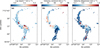 |
Fig. A Moment maps of H2 CO(30,3−20,2). Panel a: Velocity-integrated intensity (moment 0) map over [50, 60] km s−1. Panel b: Mean velocity (moment 1) map. Panel c: Velocity dispersion (moment 2) map. The ALMA beam size is shown at the bottom left. Note that for all panels, only effective emission above 3 σH2CO(σH2CO=0.004 Jy beam−1) is visualized. |
Appendix B Core extraction
As displayed in Fig. B, dust continuum emission at 1.3 mm is highly structured. We extracted compact cores from the 1.3 mm continuum image using the widely-adopted source-extraction algorithm astrodendro. As inputs to astrodendro, the following parameters were used: min_value =5 σ1.3 mm (the minimum intensity considered in the analysis), min_delta = 1 σ1.3 mm (the minimum spacing between isocontours), and min_npix = 18 (the minimum number of pixels contained within a structure). Here, the min_npix parameter was determined as  , where the synthesize beam size of 1.3 mm observations corresponds to θmaj=0.71′′ and θmin=0.59′′), and Apix is the pixel area. As a result, we identified 26 dense cores from the 1.3 mm continuum image (Fig. B). Their measured parameters (see Sect. 3) by the algorithm are listed in Table 2.
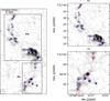 |
Fig. B Extraction results of dense cores from ALMA-alone 1.3 mm continuum emission using the astrodendro algorithm. The contours outline the identified cores while the ellipses fit them. The synthetic beam of 0.60′′ × 0.58′′ and the scale bar of 0.5 pc are shown in the lower and upper left corners, respectively. |
Appendix C Evolutionary stages of cores
We adopt the evolutionary classification (prestellar or protostellar) for the 26 dense cores in I19074 from Cheng et al. (2024). The classification criteria were based on the detection of molecular outflows and warm gas tracers. Using lines such as CO 2−1, SiO 5−4, SO, H2 CO, and CH3 OH, 3 cores were identified as protostellar based on clear molecular outflows. To further identify star-forming activity, we complemented this with a search for emission from “warm core” tracers: the H2 CO warm transitions (32,2−22,1)(218.475632 GHz, Eu/k=68.09 K),(32,1−22,0)(218.760066 GHz, Eu/k=68.11 K), CH3 OH(42,2−31,2)(218.440063 GHz, Eu/k=45.56 K), and HC3 N 24−23(218.324723 GHz, Eu/k=130.98 K). These lines, characterized by high upper-state energies, are excited by internal heating from protostars. For each core, integration maps of these lines are shown in (Figs. C1–C4). A core was classified as “warm” if it showed a compact, centrally-peaked emission peak exceeding 4 σ in any of these lines. In summary, of the 26 cores, 6 are protostellar (identified via outflows and/or warm tracers), and the remaining 20 are classified as prestellar candidates.
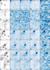 |
Fig. C1 Figure for cores 1-7 showing evolutionary stage classification (prestellar: green; protostellar: orange) based on outflow and warm gas tracers. Left column displays 1.3 mm continuum (grayscale with black contours at 1.3 × 10⁻⁴ Jy beam−1 km s−1 ×(5, 10, 20, 40, 80, 160) overlaid with CO (2-1) outflow maps (blue/red contours at 0.045 Jy° beam km s−1 ×(5, 10, 20, 40, 80, 160), integrated over 5 to 15 kms from systemic velocity; arrows indicate flow direction). Columns 2-5 show integrated intensity maps of molecular line tracers (5 km s−1 integration width) with contour levels σline ×(5, 10, 20, 40, 80). In all panels the core is indicated by one ellipse, with green color indicating prestellar, orange indicating protostellar. |
Appendix D Maps of velocity, rotation temperature and line width of N H3 (1−1)
Figure D shows the rotation temperature, the mean velocity and the line-width maps derived from NH3(1−1) observations by Lu et al. (2014).
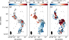 |
Fig. D Parameter maps derived from VLA NH3 (1-1) observations at 22 GHz, overlaid with contours of ALMA 1.3 mm continuum emission. Panel a: Rotation temperature map. Panel b: Mean velocity (moment 1) map. Panel c: line width map. The VLA beam size is shown at the bottom left. In each panel, the black contours are [3, 5, 10, 20, 40, 80, 160] × σ1.3 mm(σ1.3 mm=0.1 mJy beam−1). |
Appendix E Derived parameters of the classical H II region in 19074
The I19074 region hosts an associated classical H II region (see Sect. 1 and Fig. 1). Based on the observational data presented in Sect. 2, two fundamental physical parameters of the H II region can be derived, including the electron temperature (Te) and the production rate of Lyman continuum photons (NLym).
The electron temperature of H II regions has been empirically found to be correlated with the Galactocentric distance, RGal, (Quireza et al. 2006) following
 (E.1)
with D being the distance to the source, R0=8.5 kpc the distance from the Sun to the Galactic center, and l the Galactic longitude of the source. For I19074, RGal is estimated to be ∼6.3 kpc, yielding Te ∼7600 K.
(E.1)
with D being the distance to the source, R0=8.5 kpc the distance from the Sun to the Galactic center, and l the Galactic longitude of the source. For I19074, RGal is estimated to be ∼6.3 kpc, yielding Te ∼7600 K.
Assuming the H II region is in ionization equilibrium at this temperature, the NLym parameter can be calculated (Kurtz et al. 1994) as
 (E.2)
For I19074, the integrated 20 cm continuum flux density is Sv ≈ 0.2 Jy at a frequency of v ≈ 1.4 GHz over the angular size of θ=36.98′′ of the H II region. We therefore derived NLy ≈ 1.6 × 1048 ph s−1. According to Martins et al. (2005), the estimated NLy(log NLy ≈ 48.41) corresponds to one or more early-type O8-O8.5 V stars responsible for ionizing the H II region. However, this value should be considered a lower limit, as it does not account for potential losses of Lyman continuum photons due to dust absorption within the H II region or leakage through low-density channels (e.g., toward the northwest).
(E.2)
For I19074, the integrated 20 cm continuum flux density is Sv ≈ 0.2 Jy at a frequency of v ≈ 1.4 GHz over the angular size of θ=36.98′′ of the H II region. We therefore derived NLy ≈ 1.6 × 1048 ph s−1. According to Martins et al. (2005), the estimated NLy(log NLy ≈ 48.41) corresponds to one or more early-type O8-O8.5 V stars responsible for ionizing the H II region. However, this value should be considered a lower limit, as it does not account for potential losses of Lyman continuum photons due to dust absorption within the H II region or leakage through low-density channels (e.g., toward the northwest).
As discussed in Sect. 4, the H II region appears to be undergoing expansion. If the expansion occurs into a homogeneous medium, the dynamical age of the H II region can be estimated following Dyson & Williams (1980):
 (E.3)
(E.3)
![Mathematical equation: $t_{\mathrm{dyn}}=\frac{4}{7} \frac{R_{\mathrm{st}}}{C_{\mathrm{H}{{\small{\mathrm{II}}}}}}\left[\left(\frac{R_{\mathrm{IF}}}{R_{\mathrm{st}}}\right)^{7 / 4}-1\right],$](/articles/aa/full_html/2025/12/aa56572-25/aa56572-25-eq164.png) (E.4)
where Rst is the radius of the Strömgren sphere, nH,0 is the initial number density of the ambient neutral gas, αB=2.6 × 10⁻¹³(T/104 K)−0.7 cm3 s−1 (Kwan 1997) is the case B recombination coefficient, CHII ≈ 10 km s−1 is the isothermal sound speed of the ionized gas, and RIF is the radius of the ionization front, approximated here as the observed H II region radius. We assume here that the southern Fs filamentary segment was not significantly affected by the northern H II region, and can thus be treated roughly to represent the initial conditions prior to the onset of the H II region expansion. We therefore estimated initial particle density of nH,0 using the H2 number density of clump 1 in Fs, yeilding nH,0 ∼2.2 × 104 cm−3(nH,0=2 nH2). With the derived NLy, the dynamical age is estimated to be tdyn ≈ 0.4 Myr.
(E.4)
where Rst is the radius of the Strömgren sphere, nH,0 is the initial number density of the ambient neutral gas, αB=2.6 × 10⁻¹³(T/104 K)−0.7 cm3 s−1 (Kwan 1997) is the case B recombination coefficient, CHII ≈ 10 km s−1 is the isothermal sound speed of the ionized gas, and RIF is the radius of the ionization front, approximated here as the observed H II region radius. We assume here that the southern Fs filamentary segment was not significantly affected by the northern H II region, and can thus be treated roughly to represent the initial conditions prior to the onset of the H II region expansion. We therefore estimated initial particle density of nH,0 using the H2 number density of clump 1 in Fs, yeilding nH,0 ∼2.2 × 104 cm−3(nH,0=2 nH2). With the derived NLy, the dynamical age is estimated to be tdyn ≈ 0.4 Myr.
However, this estimate should be interpreted with caution, as the actual expansion occurs in a non-uniform medium rather than a strictly homogeneous one as observed in I19074 where the filamentary Fn segment is located in the east of the H II region while the western side appears relatively devoid of dense material. As such, ionized gas in I19074 would be expanding at a lower velocity than 10 km s−1 toward the western and dense side of the H II region due to large amount of ionized gas escaping toward the eastern low density side. As discussed in Sect. 4.1, the present expansion velocity of the H II region is estimated to be about 1.5 km s−1. Taking the average of these two velocity estimates yields a revised dynamical age of tdyn ≈ 0.7 Myr. This timescale is comparable to the fragmentation time of the Fn filamentary segment (see Sect. 3.3), suggesting that the expansion of the H,II region may have had sufficient time to influence the formation and evolution of Fn.
Moreover, if the expansion of the H II region is primarily driven by ionizing radiation from one or more massive stars, the kinetic energy of the expanding molecular shell resulting from energy transfer via the Lyman continuum can be estimated (Lasker 1967; Xu et al. 2018):
![Mathematical equation: $E_{\mathrm{k}}=\frac{4}{3} \pi n_{H, 0} m_{H} C_{\mathrm{H}\ \small{\mathrm{II}}}^{2} R_{\mathrm{st}}^{3 / 2}\left[\left(\frac{7}{4} C_{\mathrm{H}\ \small{\mathrm{II}}} R_{\mathrm{st}}^{3 / 4} t_{\mathrm{dyn}}+R_{s t}^{7 / 4}\right)^{6 / 7}-R_{s}^{3 / 2}\right].$](/articles/aa/full_html/2025/12/aa56572-25/aa56572-25-eq165.png) (E.5)
For the I19074 region, we estimated Ek ≈ 4.9 × 1046 erg. This value is in good agreement with the observed kinetic energy of the northern filamentary segment,
(E.5)
For the I19074 region, we estimated Ek ≈ 4.9 × 1046 erg. This value is in good agreement with the observed kinetic energy of the northern filamentary segment,  , where vexp ∼1.5 km s−1 was assumed (see Sect. 4.1). This agreement suggests that ionizing radiation from the massive stars within the H II region of I19074 provides sufficient energy to drive the expansion of the molecular gas shell.
All Tables
All Figures
|
Fig. 1 Spitzer three-color image of the I19074 region in the mid-infrared bands (blue: 3.6 μm, green: 4.5 μm, red: 8.0 μm). The white contours represent 1.2 mm dust continuum emission from the MAMBO survey (Beuther et al. 2002), while the black contours indicate 20 cm radio continuum emission from the EFFLSBRG survey (Winkel et al. 2016). Contour levels for the 20 cm radio emission (black) start at 5 σ20 cm(σ20 cm=0.2 mJy beam−1) and increase in steps of 5 σ20 cm. The 1.2 mm dust emission (white) is contoured at [3, 5, 7, 9, 15, 21, 27, 33] × σ1.2 mm, where σ1.2 mm=7 mJy beam−1. Cyan circles and blue plus mark the positions of identified compact sources and UC H II region by Lu et al. (2018). The cyan band outlines the S-shaped filament connecting the compact sources. The (synthesized) beams for the MAMBO (11′′ × 11′′) and ALMA (0.60′′ × 0.58′′) observations are shown in the lower-left and lower-right corners, respectively. The dashed loop shows the ALMA mosaic field. A scale bar of 0.5 pc is shown in the top right corner. |
| In the text | |
|
Fig. 2 Left: Combined ALMA 1.3 mm continuum map of I19074 with 26 cores overlaid (gray ellipses). The gray dashed contour marks the 2 σ1.3 mm boundary. Protostellar cores are marked as green stars. Right: ALMA-alone 1.3 mm continuum map with black contours ([3, 5, 10, 20, 40, 80, and 160] × σ1.3 mm, σ1.3 mm=0.08 mJy beam−1). Hierarchical structures Fn and Fs are bounded by the gray dashed contour at the 2 σ1.3 mm level. Blue plus marks the position of identified UC H II region by Lu et al. (2018). The synthesized beam and 0.5 pc scale bar are shown in right corners. |
| In the text | |
|
Fig. 3 Spatial distribution of dense cores in I19074. The background shows ALMA 1.3 mm continuum emission. Blue dots mark core locations and the yellow solid line denotes the minimum path connecting these elements, given by the MST algorithm. The green dashed ellipses indicate clumps. The blue dashed contours are at [9, 15, 21, 27, and 33]× σ1.2 mm. The synthetic beam of 0.60′′ × 0.58′′ for ALMA observations and the scale bar of 0.5 pc are shown in right corners. |
| In the text | |
|
Fig. A Moment maps of H2 CO(30,3−20,2). Panel a: Velocity-integrated intensity (moment 0) map over [50, 60] km s−1. Panel b: Mean velocity (moment 1) map. Panel c: Velocity dispersion (moment 2) map. The ALMA beam size is shown at the bottom left. Note that for all panels, only effective emission above 3 σH2CO(σH2CO=0.004 Jy beam−1) is visualized. |
| In the text | |
|
Fig. B Extraction results of dense cores from ALMA-alone 1.3 mm continuum emission using the astrodendro algorithm. The contours outline the identified cores while the ellipses fit them. The synthetic beam of 0.60′′ × 0.58′′ and the scale bar of 0.5 pc are shown in the lower and upper left corners, respectively. |
| In the text | |
|
Fig. C1 Figure for cores 1-7 showing evolutionary stage classification (prestellar: green; protostellar: orange) based on outflow and warm gas tracers. Left column displays 1.3 mm continuum (grayscale with black contours at 1.3 × 10⁻⁴ Jy beam−1 km s−1 ×(5, 10, 20, 40, 80, 160) overlaid with CO (2-1) outflow maps (blue/red contours at 0.045 Jy° beam km s−1 ×(5, 10, 20, 40, 80, 160), integrated over 5 to 15 kms from systemic velocity; arrows indicate flow direction). Columns 2-5 show integrated intensity maps of molecular line tracers (5 km s−1 integration width) with contour levels σline ×(5, 10, 20, 40, 80). In all panels the core is indicated by one ellipse, with green color indicating prestellar, orange indicating protostellar. |
| In the text | |
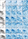 |
Fig. C2 Same as Fig. C1, but for core 8–14. |
| In the text | |
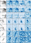 |
Fig. C3 Same as Fig. C1, but for core 15–21. |
| In the text | |
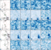 |
Fig. C4 Same as Fig. C1, but for core 22–26. |
| In the text | |
|
Fig. D Parameter maps derived from VLA NH3 (1-1) observations at 22 GHz, overlaid with contours of ALMA 1.3 mm continuum emission. Panel a: Rotation temperature map. Panel b: Mean velocity (moment 1) map. Panel c: line width map. The VLA beam size is shown at the bottom left. In each panel, the black contours are [3, 5, 10, 20, 40, 80, 160] × σ1.3 mm(σ1.3 mm=0.1 mJy beam−1). |
| In the text | |
Current usage metrics show cumulative count of Article Views (full-text article views including HTML views, PDF and ePub downloads, according to the available data) and Abstracts Views on Vision4Press platform.
Data correspond to usage on the plateform after 2015. The current usage metrics is available 48-96 hours after online publication and is updated daily on week days.
Initial download of the metrics may take a while.