| Issue |
A&A
Volume 704, December 2025
|
|
|---|---|---|
| Article Number | A254 | |
| Number of page(s) | 16 | |
| Section | Extragalactic astronomy | |
| DOI | https://doi.org/10.1051/0004-6361/202556579 | |
| Published online | 12 December 2025 | |
Molecular gas in a system of two interacting galaxies overlapping on the line of sight
1
LUX, Observatoire de Paris, Sorbonne Université, Université PSL, CNRS, F-75014 Paris, France
2
Centre for Astrophysics and Supercomputing, Swinburne University of Technology, PO Box 218 Hawthorn, VIC 3122, Australia
3
ARC Centre of Excellence for All Sky Astrophysics in 3 Dimensions (ASTRO 3D), Australia
4
Steward Observatory, University of Arizona, 933 N Cherry Av, Tucson, AZ 85721, USA
5
Collège de France, 11 Place Marcelin Berthelot, F-75005 Paris, France
★ Corresponding author: This email address is being protected from spambots. You need JavaScript enabled to view it.
Received:
24
July
2025
Accepted:
6
October
2025
Abstract
Galaxy interactions can disturb gas in galactic discs, compress it, excite it, and enhance star formation. An intriguing system likely consisting of two interacting galaxies overlapping on the line of sight was previously studied through ionised gas observations from the integral-field spectrograph Mapping Nearby Galaxies at APO (MaNGA). A decomposition into two components using MaNGA spectra, together with a multi-wavelength study, allowed us to characterise the system as a minor-merger with interaction-induced star-formation, and perhaps active galactic nucleus (AGN) activity. We used new interferometric observations of the CO(1–0) gas of this system from the NOrthern Extended Millimeter Array (NOEMA) to confront and combine the spatially resolved ionised and molecular gas observations. Mock NOEMA and MaNGA data are computed from simulated systems of two discs and compared to the observations. The NOEMA observations of the molecular gas, dynamically colder than the ionised gas, help to constrain the configuration of the system, which we revisited as a major merger. A combination of ionised and molecular gas data allowed us to study the star-formation efficiency of the system.
Key words: galaxies: evolution / galaxies: interactions / galaxies: kinematics and dynamics / galaxies: spiral / galaxies: star formation
© The Authors 2025
 Open Access article, published by EDP Sciences, under the terms of the Creative Commons Attribution License (https://creativecommons.org/licenses/by/4.0), which permits unrestricted use, distribution, and reproduction in any medium, provided the original work is properly cited.
This article is published in open access under the Subscribe to Open model. This email address is being protected from spambots. You need JavaScript enabled to view it. to support open access publication.
1. Introduction
Galaxy interactions are sites of possible gas compression, the enhancement of star formation, and the triggering of active galactic nucleus (AGN) activity. The molecular gas is a particularly interesting tracer to study the dynamics of such systems, as it is dynamically cold. It can be observed through the emission of the CO molecule in a large range of redshifts.
Combining resolved molecular-gas and star-formation-rate (SFR) observations, Kennicutt–Schmidt (KS) relations (Schmidt 1959; Kennicutt 1998) were obtained in local galaxies (Leroy et al. 2008; Bigiel et al. 2008). Similar studies at higher redshift were also performed, as by Freundlich et al. (2013), around redshift 1.2. For example, it is possible to estimate the SFR from ionised gas, and in particular the Hα emission of recombining hydrogen. Studies such as ALMaQUEST (Lin et al. 2019) have used ionised-gas- and molecular-gas-resolved observations in low-redshift galaxies to derive star-formation efficiency and departure from the main sequence of star-forming galaxies (MS), relating SFR and stellar mass.
This work focused on J221024.49+114247.0, a z = 0.09228 (according to the NASA Sloan Atlas catalogue) system that was identified as showing double-peaked emission lines of ionised gas in the 3″ SDSS fibre by Maschmann et al. (2020). Double-peaked emission lines have a variety of possible origins, including disc rotation, gas outflows, and galaxy mergers (Maschmann et al. 2023). In the case of J221024.49+114247.0, a detailed study was performed in Mazzilli Ciraulo et al. (2021), combining integral-field-unit (IFU) MaNGA observations (Bundy et al. 2015) of the ionised gas (with the identifier MaNGA-ID 1-114955, or, in Plate-IFU, 7977-12701), IRAM 30 m observations of the CO(1–0) and CO(2–1) emission, and VLA radio observations. Through the decomposition of the spatially resolved MaNGA observations of the ionised gas, it is possible to isolate two different kinematic components corresponding to two counter-rotating galactic discs overlapping on the line of sight. New interferometric observations of the molecular gas were performed by the NOrthern Extended Millimeter Array (NOEMA), in the CO(1–0) line, yielding the spatially resolved molecular content of the system; this can be compared with the spatially resolved ionised-gas data.
After a presentation of the system of interest and a summary of related previous works in Sect. 2, we study its molecular gas content with NOEMA and the relationship between this gas and SFR obtained through Hα in Sect. 3. We then explain how we modelled the system kinematically with two discs and recovered the contribution of each galaxy to the molecular gas content and to the emission lines of ionised gas in Sect. 4; we discuss our results in Sect. 5. Throughout this work, we assumed a flat ΛCDM cosmology with ΩM = 0.3, ΩΛ = 0.7 and H0 = 70 km/s/Mpc.
2. J221024.49+114247.0
The system J221024.49+114247.0 appears in optical and near-infrared bands as a perturbed galaxy. Figure 1 shows a composite Legacy image (Dey et al. 2019) and a CFHT MegaPipe (Gwyn 2008) r-band image. It has a redshift of z = 0.09228 according to the NASA Sloan Atlas catalogue. The SDSS fibre is represented as a dashed black circle in Fig. 1 and other maps of this work. Maschmann et al. (2020) identified double-peaked emission lines in this fibre. According to the spectral-energy-distribution (SED) fitting of Salim et al. (2016), using a Chabrier initial mass function (IMF), the stellar mass is 1.6 × 10¹¹ M⊙ and the SFR is 14 M⊙/yr.
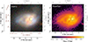 |
Fig. 1. Legacy composite image (left) and log10 of MegaPipe image (right), from MegaCam on CFHT. The 3″ SDSS fibre is over-plotted with a dashed black circle. |
As detailed in Mazzilli Ciraulo et al. (2021), the system exhibits spiral features, possible tidal features (especially in the north-west, as best seen in the CFHT MegaPipe image of Fig. 1), and what appears to be a dust lane from south-east to north-west. Coordinates relative to the centre of the SDSS fibre are shown in arcseconds and in kiloparsecs1.
Using MaNGA observations, Mazzilli Ciraulo et al. (2021) concluded that the system is a minor merger (with a mass ratio 1:9) of two disc galaxies overlapping on the line of sight: a ‘main galaxy’, extending across the whole spatial extent of the observed system, and a ‘secondary galaxy’, which is smaller and likely aligned with the dust lane visible in the legacy composite image of Fig. 1. Their study was based on decompositions of both stellar and gas emission-line MaNGA data into two components in each spaxel. For gas emission lines, both single- and double-Gaussian fits of emission lines were performed in each spaxel, with limits on the variation of fitted parameters between neighbouring spaxels, and an F-test determined the best of single- and double-Gaussian fits for each spaxel. The mass ratio of 1:9 was estimated from the rotation velocities obtained from the histogram of stellar or gas velocities corrected from the estimated inclinations and from the estimated spatial extents of the two discs. The spectral index obtained from radio data was not conclusive regarding possible AGN activity. This system is a member of the 69 double-peaked galaxy sample of Mazzilli Ciraulo et al. (2024), where it is labelled G61. In Mazzilli Ciraulo et al. (2024), G61 is shown to belong to the blue cloud with an apparent NUV-r magnitude of 2.4 and an intrinsic corrected NUV-r magnitude (corrected for dust attenuation) of 2. Its r-band absolute magnitude Mr is of −22.7. It is also shown to belong to the star-forming sequence of the intrinsic NUV-r magnitude versus specific SFR diagram (see Fig. 10 of Mazzilli Ciraulo et al. 2024). Its stellar index Dn 4000 is below 1.5 in most of the galaxy, indicating young stellar populations (see Fig. G2 of Mazzilli Ciraulo et al. 2024).
Mazzilli Ciraulo et al. (2021) used the MaNGA DR16 data to perform emission-line fitting for this system. They used the VOR10-GAU-MILESHC model cube from the MaNGA data analysis pipeline (DAP) (Westfall et al. 2019), with the same Voronoi binning for stellar and gaseous components, because they also performed a study of the stellar component with Nburst (Chilingarian et al. 2007a,b). MaNGA DR17 data have become available, with a new flux calibration and new stellar and emission-line fittings. In the present work, we focused on the study of emission lines (which we compare to the molecular gas data) and thus used the DR17 HYB10-MILESHC-MASTARSSP cube with a hybrid binning scheme (Voronoi binning for stars but not for gas), which is recommended in the case of study of the sole emission lines. After removing the stellar contribution using the DAP model cube and correcting for Galactic extinction, we performed the same fitting procedure on the emission lines as in Mazzilli Ciraulo et al. (2021). These fits were used to produce the maps and diagrams of the next section (Sect. 3) and Appendix B.
3. Molecular gas content and star formation
We studied the molecular gas content of the system based on NOEMA CO(1–0) observations. We used MaNGA observations to compute metallicity and derive the conversion factor from CO(1–0) emission to molecular gas mass. From the surface densities of both molecular gas and SFR from MaNGA, we computed the star-formation efficiency.
3.1. NOEMA observations of CO(1–0)
Single-dish observations of J221024.49+114247.0 in CO(1–0) and CO(2-1) were performed at the IRAM 30 m telescope and presented in Mazzilli Ciraulo et al. (2021). The source was then observed in CO(1–0) by NOEMA (project S21BQ001, P.I. Barbara Mazzilli Ciraulo) at a rest frequency of 105.533 GHz during three time slots in 2021: 2.1 hours on 21 July in configuration 10D of the array, 1.1 hours on 25 July in configuration 8D+N01, and 2.6 hours on 25 November in configuration 10C. Data calibration and image deconvolution were performed with the GILDAS2 software, using natural weighting and a Hogbom cleaning on the whole field of view of 95.5″ × 95.5″. The elliptical Gaussian synthesised beam has axes of full widths at half maximum (FWHMs) of 2.92″ and 1.68″, with a 22.4° position angle. Table 1 gathers spatial-resolution details with conversions into kiloparsecs (with similar details for MaNGA observations). NOEMA velocity channels are stacked 6 × 6 to increase the signal-to-noise ratio, resulting in a velocity resolution of 34.1 km/s.
Spatial resolution of NOEMA and MaNGA observations.
Maps of the CO(1–0) line intensity, line-of-sight velocity and velocity dispersion, obtained through summations on velocity channels, are shown in Fig. 23. A threshold in flux density was applied in summations to limit the noise level4. Velocity-channel maps, with the same threshold, are shown in Fig. 4. When velocity increases, the peak flux density shifts from the south-west (bottom right of each panel) to the north-east (top left of each panel) at v ≃ 0, and then to the south-west again. A 3D view of the NOEMA cube, using the same threshold, is shown in Fig. A.1, with a link to the corresponding 3D interactive visualisation5.
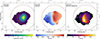 |
Fig. 2. Intensity, velocity, and velocity dispersion obtained for CO(1–0) NOEMA observations. A flux-density threshold of 1 mJy/beam is applied. We over-plot linearly spaced contours of the CO(1–0) intensity on each map. The NOEMA elliptical, Gaussian synthesised beam is represented in the bottom left corners of the panels. The IRAM 30 m CO(1–0) and CO(2–1) beams are shown in brown and yellow, respectively. The 3″ SDSS fibre is over-plotted with a dashed black circle. |
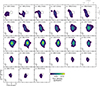 |
Fig. 4. Velocity channel maps. The 3″ SDSS fibre is over-plotted with a dashed black circle. |
The CO(1–0) NOEMA spectrum, gathered over the 30 m beam of 11 arcsec radius, is compared with the CO(1–0) 30 m spectrum, binned to the same velocity resolution, in Fig. 3. The two spectra are very similar, meaning that the interferometer does not lose flux. In Mazzilli Ciraulo et al. (2021), the CO(2–1) 30 m spectrum was also shown, exhibiting a slightly different shape from the CO(1–0) at low velocities. This CO(2–1) spectrum is also shown in Fig. 3, with the same velocity resolution. It is multiplied by 1/4 for comparison of shape with the CO(1–0) spectrum. The slight depletion at low velocities is consistent with the low-velocity part of the system being outside of the CO(2–1) beam, as visible on the velocity map of Fig. 2.
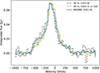 |
Fig. 3. NOEMA CO(1–0) spectrum stacked over a 22 arcsec aperture, compared to the IRAM 30 m spectra, at the same velocity resolution. |
3.2. Surface density of molecular gas
The surface density of molecular gas is obtained through the computation of the intrinsic CO luminosity and a luminosity-to-molecular-gas-mass conversion factor. The intrinsic CO luminosity is obtained from the velocity-integrated transition-line flux, FCO(1 → 0), by
 (1)
(1)
where νrest = 115.271 GHz is the rest CO(1–0) line frequency and DL is the luminosity distance (Solomon et al. 1997). The total molecular gas mass is
 (2)
(2)
with αCO being the CO(1–0) luminosity-to-molecular-gas-mass conversion factor, defined to include helium in the molecular mass (Mmol gas = 1.36 MH2). This factor has a value empirically established in the Milky Way of αG = 4.36 ± 0.9 M⊙(K km s−1 pc2)−1, based on assumptions including a solar metallicity for the gas.
The conversion factor αCO is a decreasing function of the metallicity of the gas, which is parametrised, for example, by the oxygen-abundance as log Z = 12 + log(O/H). We computed this gas-phase metallicity through the O3N2 index ![Mathematical equation: $ \mathrm{O_3N_2}={ \rm [O III] \lambda 5007/H \beta )/([N II] \lambda 6583/ H \alpha}) $](/articles/aa/full_html/2025/12/aa56579-25/aa56579-25-eq3.gif) using the calibration of Pettini & Pagel (2004): log Z = 8.73 − 0.32 logO3N2. We estimate a single value of this factor for the system through stacked Gaussian-emission-line fluxes given in the MaNGA DAP catalogue for a stacking performed in an elliptical aperture of the semi-major axis the effective radius in the r band of the system, as obtained from a Petrosian analysis. The corresponding O3N2 metallicity is log Z = 8.65. Maps of the fluxes of Hα, Hβ, [OIII]λ5007, and [NII]λ6583 with a minimum signal-to-noise ratio (S/N) of 3 are shown in Fig. B.1, with the gas-phase metallicity map from the O3N2 index computed from these maps. The aperture used in the DAP is shown in orange in the gas-phase metallicity panel of Fig. B.1. We used this log Z = 8.65 gas-phase metallicity value to compute the luminosity-to-molecular-gas-mass conversion factor because this elliptical aperture encompasses most of the CO(1–0) emission. A similar value of log Z = 8.67 is given by the DAP from the same method with a 2.5″ radius aperture; this is also shown in Fig. B.1.
using the calibration of Pettini & Pagel (2004): log Z = 8.73 − 0.32 logO3N2. We estimate a single value of this factor for the system through stacked Gaussian-emission-line fluxes given in the MaNGA DAP catalogue for a stacking performed in an elliptical aperture of the semi-major axis the effective radius in the r band of the system, as obtained from a Petrosian analysis. The corresponding O3N2 metallicity is log Z = 8.65. Maps of the fluxes of Hα, Hβ, [OIII]λ5007, and [NII]λ6583 with a minimum signal-to-noise ratio (S/N) of 3 are shown in Fig. B.1, with the gas-phase metallicity map from the O3N2 index computed from these maps. The aperture used in the DAP is shown in orange in the gas-phase metallicity panel of Fig. B.1. We used this log Z = 8.65 gas-phase metallicity value to compute the luminosity-to-molecular-gas-mass conversion factor because this elliptical aperture encompasses most of the CO(1–0) emission. A similar value of log Z = 8.67 is given by the DAP from the same method with a 2.5″ radius aperture; this is also shown in Fig. B.1.
As the gas-phase metallicity is close to the solar value, following Genzel et al. (2015), we used a correction to the Galactic value that is the geometric mean of the corrections established by Bolatto et al. (2013) and by Genzel et al. (2012), as in Mazzilli Ciraulo et al. (2021):
 (3)
(3)
The obtained value is αCO = 4.41 M⊙(K km s−1 pc2)−1. The resulting molecular-gas surface density map is shown on Fig. 5. The total observed mass of molecular gas is Mmol gas obs = 4.2 × 10¹⁰ M⊙6 (MH2 = 3.1 × 10¹⁰ M⊙, as in Mazzilli Ciraulo et al. (2021)).
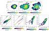 |
Fig. 5. Top row: molecular-gas surface density (left), Hα-based SFR surface density (middle) and stellar surface density (right). CO(1–0) intensity contours are over-plotted in grey. The 3″ SDSS fibre is over-plotted with a dashed black circle. Bottom row: diagrams obtained after degrading the maps to the same spatial resolution (see text). From left to right: KS diagram with 2D bins colour-coded by the number of contributing MaNGA spaxels; KS diagram with one dot per MaNGA spaxel, colour-coded by its distance to the centre of the SDSS fibre; molecular-gas surface density versus stellar surface density; and SFR surface density versus stellar surface density. In the two KS diagrams, locations of constant depletion times are shown as diagonal black lines, and as a diagonal blue line for the average depletion time of high-density molecular gas. |
The conversion factor may differ significantly from the Galactic value if the gas is in a different physical state or has a large column density (Bolatto et al. 2013). For example, the typical value assumed in ultra-luminous infrared galaxies (ULIRGs) is 0.8 M⊙(K km s−1 pc2)−1 (Downes & Solomon 1998), meaning that a lower molecular-gas mass is estimated from a given CO emission. Our system is likely composed of two galaxies with their molecular gas potentially in different states, and there may be outflows, making it all the more difficult to estimate a reliable conversion factor.
3.3. Star-formation rate from MaNGA Hα
The SFR is obtained from the Hα luminosity similarly to the derivation in Mazzilli Ciraulo et al. (2021). We computed an Hα-based SFR using Kennicutt (1998)
 (4)
(4)
which assumes a Salpeter (1955) initial mass function (IMF). Lcorr(Hα) is the luminosity of the Hα emission line corrected from dust attenuation. Lcorr(Hα) was obtained by correcting the observed luminosity Lobs(Hα) by
 (5)
(5)
where AλHα is the attenuation at the Hα rest-frame wavelength, k(λHα) is the value of the total attenuation curve at the Hα rest-frame wavelength, and E(B − V) = AB − AV is the colour excess, with AB and AV being the attenuations in the B and V bands (respectively). The total attenuation curve is parametrised, for example by O’Donnell (1994), in the Milky Way with a ratio of total-to-selective extinction in the V band:  . Using Eq. (5) applied to both Hα and Hβ, the colour excess is computed by
![Mathematical equation: $$ \begin{aligned} E(B-V) = \dfrac{2.5}{k(\lambda _{\rm H\beta }) - k(\lambda _{\rm H\alpha )})} \, \mathrm{log}_{10} \left[ \frac{(\mathrm H\alpha / H\beta )_{obs}}{2.86}\right], \end{aligned} $$](/articles/aa/full_html/2025/12/aa56579-25/aa56579-25-eq8.gif) (6)
(6)
where (Hα/Hβ)obs is the Balmer decrement, the ratio of observed Hα and Hβ luminosities (both affected by dust absorption), and an intrinsic (with no effect from dust) Balmer decrement, Hα/Hβ of 2.86 is assumed, which corresponds to a temperature of T = 104 K and an electron density of ne = 102 cm−3 for a case B recombination (Osterbrock & Ferland 2006). This computation of SFR by a correction of Hα luminosity may not correct for the whole effect of dust absorption if Lyman continuum photons emitted by stars are directly absorbed by dust and are therefore not accounted for.
The map of the colour excess E(B − V) is shown in Fig. B.1. It is computed from the Hα and Hβ flux maps of the same figure and from the attenuation curve of O’Donnell (1994) with RV = 3.1. The map of SFR surface density is shown in Fig. 5. A total SFR of 19 M⊙/yr is obtained. Removing the AGN contribution fAGN to the Hα flux estimated by the method of Jin et al. (2021) gives an only slightly lower total SFR of 18 M⊙/yr7.
3.4. Galaxy baryonic content and star-formation diagnostics combining NOEMA and MaNGA
Using the stellar mass M* = 1.6 × 10¹¹ M⊙ found by Salim et al. (2016) and the Hα-based SFR obtained in the previous subsection, one can compute  , where SFRMS(z, M*) is the SFR of the MS at redshift z and stellar mass M*, as parametrised by Speagle et al. (2014). The system is log10δMS = 0.46 dex above the MS. Using the molecular-gas mass Mmol gas obs computed in Sect. 3.2, the molecular-gas-mass-to-stellar-mass ratio is μ = 0.26 and the global depletion time,
  is 2.2 Gyr. tdepl, is 0.66 dex above the expected value at δMS obtained from the parametrisation by Tacconi et al. (2018).8
The angular resolutions of both MaNGA and NOEMA observations (spaxel size and PSF or beam FWHM) are given in Table 1. To compare the surface densities of SFR and molecular gas, we convolved the molecular-gas map by the NOEMA beam rotated by 90° to emulate a circular beam, Bcommon, of FWHM  , with lmajor (resp. lminor) being the FWHM of the NOEMA major (resp. minor) axis. We also convolved the MaNGA maps by a circular Gaussian beam of FWHM
  , with lPSF being the FWHM of the MaNGA PSF, to also emulate a convolution with Bcommon. Spatial resolution is thus degraded in both maps to the same beam. We then reprojected the molecular gas map on the MaNGA bins9. The resulting KS diagram, showing ΣSFR as a function of Σmol gas, is shown in Fig. 5. The left version of the diagram represents the number of MaNGA spaxels falling into a 2D bin of the KS space, and the right version represents dots corresponding to MaNGA spaxels, colour-coded by their distance to the centre of the SDSS fibre. Black lines show locations of constant molecular-gas depletion times,
  , of 100 Myr, 1 Gyr, and 10 Gyr. The average depletion time of the densest central parts, computed as the average of depletion times of MaNGA spaxels with a surface density larger than 100 M⊙/pc2, is of 2.5 Gyr, and the corresponding star-formation efficiency,
  , is 0.04/[100 Myr] (4%). The larger scatter in the KS diagrams at low molecular-gas surface density may, besides the uncertainty in αCO, reflect the more likely under-estimation of CO(1–0) flux and higher relative error in regions where the CO(1–0) flux densities are close to the spatially uniform threshold value that was adopted. The surface densities of molecular gas and SFR are also shown as a function of the stellar density obtained from the MaNGA value-added catalogue Firefly (Neumann et al. 2022; Goddard et al. 2017). These surface densities appear to be correlated (with slopes of 1.5 and 1 of fits, shown as blue lines, obtained by linear regressions for the molecular gas and SFR, respectively), similarly to the results on a molecular-gas MS and a resolved star-formation MS obtained in Lin et al. (2019). The correlation found for all the diagrams of Fig. 12, however, partly comes from the large size of Bcommon (FWHM of 3.4″) compared to the angular size of the CO(1–0) emission.
The surface densities used in the bottom row of Fig. 5 were not corrected for inclination because of the complexity of the system, likely consisting of two superposed discs with different inclinations. The axis ratio of the Petrosian analysis of the r band provided in the MaNGA DAP catalogue is 0.74. The inclination deduced from this ratio is about 43° by modelling the system as an oblate spheroid with an intrinsic axis ratio, q0, between 0 and 0.2 (so that the inclination i satisfies  (Hubble 1926)). Using this value would shift all plotted quantities by the same amount of −0.13 dex (in particular, this would not impact estimates of depletion times).
4. Modelling the system with two disc galaxies
In the following, we discuss the double-Gaussian fitting method of MaNGA emission lines used to separate the system into two discs in Mazzilli Ciraulo et al. (2021) and then present a modelling with two input discs whose parameters are constrained by a comparison to the observations. We started by applying this method to the molecular gas, which is dynamically colder and whose observations have a better spectral resolution, in order to constrain parameters. We then used the obtained parameters to separate the contributions of the two discs to the MaNGA spectra. SFE diagnostics and ionisation properties for the two individual modelled discs were then obtained.
4.1. Single- and double-Gaussian fits of MaNGA spectra
Figure 6 shows the velocity and velocity maps of ionised gas obtained with the procedure used in Mazzilli Ciraulo et al. (2021), in its single-Gaussian version. At each spaxel, emission lines (Balmer and other lines) were constrained to have the same central velocity and the same velocity dispersion, after removing the instrumental line-spread-function (LSF), and this fit is performed on the whole galaxy with constraints on the variation of amplitude, central velocity, and velocity dispersion coming from the values in neighbouring spaxels (as explained in Sect. 2, we used the now available MaNGA DR17 HYB10-MILESHC-MASTARSSP cube instead of the DR16 VOR10-GAU-MILESHC cube used in Mazzilli Ciraulo et al. 2021). This determination of velocity for ionised gas through Gaussian fitting is different from the determination for molecular gas from the computation of the first moment, making a direct comparison between the ionised-gas velocity map and the molecular-gas velocity map of the middle panel of Fig. 2 difficult. Both maps, however, show the same feature of the highest velocity gas at and around the location of the SDSS fibre. Ionised-gas velocity dispersion is larger than the molecular-gas one, as expected for a warmer component (as for the velocity, the determination is also different than for the molecular gas).
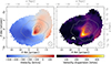 |
Fig. 6. Velocity and velocity dispersion of Hα from the Gaussian-fit procedure. |
In Mazzilli Ciraulo et al. (2021), the decomposition into two discs through the double-Gaussian fitting of ionised-gas emission lines procedure allowed us to isolate emission-line flux maps and velocity maps for the two individual components. The assumption made for this decomposition was that for each spaxel where a double-Gaussian fit was better than a single-Gaussian fit (according to an F test), each of the two Gaussians corresponded to one of the two galaxies. For spaxels in which a single-Gaussian fit was better, the Gaussian was assumed to correspond to the larger galaxy. A fitting procedure of the stellar component also allowed us to separate two distinct stellar components. The inclinations of the gas discs were estimated from the shapes of ellipses fitting emission-line maps. The lengths of the minor and major axes were not very well defined, especially for the secondary galaxy whose maps had shapes departing significantly from an ellipse. The rotation velocities Vrot were estimated by  , with W defined as the difference between the 90th and 10th percentile points of the velocity histogram, and i the previously determined inclination. The dynamical masses were estimated by Mdyn = Vrot2R/G with R the maximum radius where Hα is detected. The parameters found by Mazzilli Ciraulo et al. (2021) are listed in Table 2.
Parameters found by Mazzilli Ciraulo et al. (2021).
The double-Gaussian fitting procedure is not always able to properly separate the two discs. Double peaks can appear in spectra of spaxels near the centre of discs because of rotation (e.g. Maschmann et al. 2023). The large velocity dispersion of ionised gas and the widening of emission lines by the MaNGA LSF worsens the problem.
4.2. Modelling from the CO(1–0) NOEMA observations
From a simple analysis illustrated in Fig. 7, it appears that if the CO(1–0) emission originates from two superimposed rotating discs, the molecular gas cannot be axisymmetrically distributed in each disc with an axisymmetric CO-to-molecular gas conversion factor in each disc. In the case of an axisymmetric distribution of molecular gas and an axisymmetric conversion factor, the spectrum is symmetric around the velocity of the centre of mass of the galaxy (systemic velocity). The position-velocity diagrams (shown in Fig. 7, integrated on declination or RA), in which the characteristic shapes of emission of discs in rotation can be identified, allowed us to isolate two parts of the velocity distribution, which are most likely due to half of only one of the supposed discs: the lowest and highest velocity parts of the spectrum. By reconstructing the spectrum of each galaxy by symmetry with regard to an assumed systemic velocity, and by then summing the two obtained spectra, it is not possible to obtain the observed spectrum for any values of systemic velocities such that the extent of the individual spectra imply reasonable (< 300 km/s) rotation velocities. There is too much emission from gas at intermediate velocities. Some clumpy distribution of the molecular gas may explain this asymmetry. Some variation in metallicity or in the physical properties of the molecular gas may also make the conversion factor vary. Both molecular discs or one of them may be disturbed by a tidal interaction, resulting in an asymmetric distribution of the molecular gas. Some tidal features such as a tail or a bridge may be present. Finally, there may be some molecular outflow.
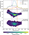 |
Fig. 7. Attempt to reconstruct the observed spectrum, assuming there are two discs, that each one has a half part accounting for the CO(1–0) emission at the lowest or highest observed velocities, and that the CO(1–0) emission of each disc is symmetric with regard to its minor kinematic axis. The violet (resp. orange) line is an example of systemic velocity for the first (resp. second) disc, with the spectrum of the disc in the same colour in the top panel. Top: NOEMA spectrum; discs’ spectra reconstructed by symmetry and their sum. Middle: NOEMA cube integrated on declination. Bottom: NOEMA cube integrated on RA. |
We realised mock NOEMA cubes with two molecular-gas discs superimposed on the line of sight. We first generated discs from particles of positions and velocities adjusted to a set of chosen parameters. We modelled gas discs with a Miyamoto & Nagai (1975) density profile:
![Mathematical equation: $$ \begin{aligned} \rho _d(R,z) = \left( \dfrac{h^2 M}{4 \pi } \right) \dfrac{a R^2 + (a + 3\sqrt{z^2 + h^2}) (a + \sqrt{z^2 + h^2})^2}{\left[ R^2 + (a + \sqrt{z^2 + h^2})^2\right]^{\frac{5}{2}} (z^2 + h^2)^{\frac{3}{2}}}, \end{aligned} $$](/articles/aa/full_html/2025/12/aa56579-25/aa56579-25-eq17.gif) (7)
(7)
where M is the total mass of the disc, a is a radial scale length, and h is a vertical scale length. We set a vertical scale length of h = 100 pc for each disc. We modelled each rotation curve with a close to linear rise from R = 0 and a smooth transition to a plateau, using an error function: the circular velocity is vc(R) = Vmaxerf(R/R0), where Vmax is the plateau velocity and R0 is the transition radius from the initial rise to the plateau. The two parameters describing each rotation curve are thus the transition galactocentric radius from rise to plateau, R0, and the velocity of the plateau, Vmax. The rotation curves are shown in Fig. 8. For each disc, we set the molecular-gas radial and azimuthal velocity dispersions (σR and σϕ, respectively) to the same value σR = σϕ = 30 km/s, independent of radius for simplicity, and set the vertical velocity dispersion σz to σz = 15 km/s. We then binned the on-sky positions and line-of-sight velocities with the same spatial and velocity binning as for the observed NOEMA cube, and we then convolved each channel map with a 2D elliptic Gaussian kernel with the FWHMs of the major and minor axes of the NOEMA synthesised beam and its position angle, using radio-beam and astropy for this convolution. The value of M in Eq. (7) was set to half the total observed molecular-gas mass Mmol gas obs determined in Sect. 3.1, and the simulated molecular-gas mass per cube cell was converted into CO(1–0) flux density using the same conversion factor as the one used to compute Mmol gas obs. The simulated flux densities are thus of the same order of magnitude as the observed ones. The simulated spectra of each disc were then adjusted spaxel by spaxel as described below.
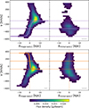 |
Fig. 8. Position–velocity diagrams of NOEMA observations centred on estimated kinematic centre of disc1 (first row) or on the estimated kinematic centre of disc2 (second row) and computed on a one-spatial-pixel-wide slice either along the major axes (first column) or the minor axes (second column) of discs. vc(R)sin(i) curves are represented on diagrams with position taken along the major axis (first column). Horizontal solid lines show the fitted systemic velocities, vsys, of the discs, and horizontal dashed lines show vsys ± Vmaxsin(i). Violet lines correspond to disc1 and orange curves to disc2. The horizontal grey lines in the bottom right corner of each panel show the projection of the elliptical Gaussian NOEMA synthesised beam on the x-axis of the panel. |
We considered a varying contribution of disc1 and disc2, the ‘main galaxy’ and ‘secondary galaxy’ of Mazzilli Ciraulo et al. (2021) (respectively), in each spaxel. With s1 and s2 being the mock spectra of disc1 and disc2, respectively, in a given spaxel, we fitted two multiplying factors, f1 and f2, one for each disc (disc1 and disc2, respectively). This was done so that the sum of the two resulting spectra, each multiplied by the corresponding fitted factor, best fits the observed spectrum, i.e. so that f1s1 + f2s2 fits the observed spectrum. This resembles the approach used in Combes et al. (2019), where a multiplicative filter was applied to the simulated cubes so that the spectrum in a spaxel is normalised to the observed spectrum in this spaxel. The fitting was performed after convolution of the mock cube by the NOEMA synthesised beam, and the fitted factors must not vary strongly on the area of the synthesised beam for this approach to be physically valid (otherwise, the contribution of the molecular gas of a given disc at a given location would be inconsistent from one spaxel to its neighbours on which it is smeared by the spatial convolution). Because of the large number of parameters and the complexity induced by the superposition on the line of sight, we fitted most parameters by eye, resorting to a least-squares method only for the local intensity of CO(1–0) emission per disc, i.e. only for the determination of f1 and f2 in each spaxel. Some of the parameters are listed in Table 3.
Parameters for models.
The NOEMA spectra were fitted after the same threshold cut as that used to produce the moment maps. The NOEMA and fitted discs’ spectra stacked over the entire system are represented in Fig. 9. Figure C.1 displays the CO(1–0) spectra and models for spaxels stacked 16 by 16 all over the system. We represent maps of the intensity, velocity, and velocity dispersion of the observations and of the model, with residuals, in Fig. 10. The first column shows the same maps as in Fig. 2, except for the colour-scale range, which is, for each row of Fig. 10, common to the first four maps. The second and third columns show the intensity, velocity and velocity dispersion of disc1 and disc2 (respectively), the fourth column shows the same quantities for the two modelled discs together, and the fifth column shows the residuals, computed as the difference between the first column (observations) and the fourth column (model). The colour scales of the residuals are centred on zero.
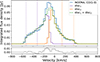 |
Fig. 9. Observation and model of CO(1–0) emission integrated on the system. Solid vertical lines show the fitted systemic velocities vsys of the discs and dashed vertical lines show vsys ± Vmaxsin(i). |
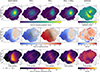 |
Fig. 10. Observations, models, and residuals of intensity, velocity, and velocity dispersion from the CO(1–0) line. Models are shown both for each disc (columns 2 and 3) and for the two superposed discs (column 4). Residuals are the observation (column 1) minus the two superposed discs (column 4). On the velocity maps of individual discs, iso-line-of-sight velocity curves are represented by dashed (resp. solid) black lines for values below (resp. above) the systemic velocity of the disc. |
Molecular-gas masses can be computed assuming, for example, the same αCO of Sect. 3. We find molecular-gas masses Mmol gas disc1 = 2.1 × 10¹⁰ M⊙ for disc1, and Mmol gas disc2 = 1.8 × 10¹⁰ M⊙ for disc2. The sum of these two masses is Mmol gas disc1 + disc2 = 3.9 × 10¹⁰ M⊙, which is slightly below the observed total mass, Mmol gas obs = 4.2 × 10¹⁰ M⊙.
4.3. Modelling applied to the MaNGA observations
We realised mock cubes for a given emission line. The velocity channels were convolved by a circular Gaussian kernel of FWHM 2.6 arcsec, accounting for the MaNGA PSF. We also performed a convolution on velocities with a 1D Gaussian kernel with the dispersion of the MaNGA line-spread function at the redshifted wavelength of the considered emission line and at each considered location (this dispersion is given in the MaNGA model cube). The conversion between wavelength λ and velocities v is done by
 (8)
(8)
where λ0 is the rest-frame wavelength of the considered emission line, and zsource is the redshift taken from the NASA Sloan Atlas catalogue. This allowed us to compare modelled and observed spectra. We kept the same parameters as for the molecular gas, except for velocity dispersion: we set the radial and azimuthal velocity dispersions to a larger value of σR = σϕ = 40 km/s and the vertical velocity dispersion to σz = 20/km/s. As for the molecular gas, we used a least-squares method to fit the contribution of each of the two discs to the spectra. The results, integrated on the system, are shown for a few emission lines in Fig. 11. In Appendix D, we show the example of the [OIII]5008 fitting: a comparison of the observed and fitted moments in Fig. D.2 and fits of spectra stacked 16 by 16 in Fig. D.1. The difference between the observed MaNGA emission lines and their fits, obtained using the system parameters found from the study of the CO(1–0) NOEMA cube, may be reduced by changing the gas disc models for the ionised gas, since the ionised-gas discs are likely different from the molecular gas discs. Also, it is possible to adopt a different radial profile for the ionised-gas velocity dispersion rather than a constant one, as assumed here for simplicity for both molecular and ionised gas. Some ionised gas outflows and tidal features may also be present. We computed the SFR of modelled disc1 and disc2 using the same dust correction as in Sect. 3, and we find a SFR of 11 M⊙/yr for disc1, a SFR of 8 M⊙/yr for disc2, and, hence, a total of 19 M⊙/yr, as the total observed SFR.
 |
Fig. 11. Observations and models of MaNGA emission lines integrated on the system. |
4.4. Star formation and gas ionisation in the discs
Figure 12 shows the KS diagrams of the two discs together, and of each individual disc (with a correction for inclination). The SFEs are similar, but a little higher in the densest parts of disc2 than in the densest parts of disc1.
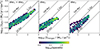 |
Fig. 12. KS diagrams. Left: Two superposed model discs, with no correction for inclination. Middle and right: Disc1 (resp. disc2), correcting for the modelled inclinations of 60 and 65 degrees, respectively. |
Baldwin, Phillips, and Terlevich (BPT) (Baldwin et al. 1981) diagrams are shown in Fig. 13, with curves defined by Kauffmann et al. (2003) and Kewley et al. (2001) separating different zones. Diagrams are shown for the double-Gaussian fit to the emission lines, which best determines the observed flux for each modelled disc component and for the sum of the two components. Each dot corresponds to a MaNGA spaxel. The ionisation in most of the spaxels seems to come from star-formation or from a composite origin (some AGN activity and/or shocks may contribute). The two discs mostly have a similar origin for their ionisation (their spaxels are in the same zones of the diagrams), but disc2 has (as found by Mazzilli Ciraulo et al. (2021)) larger [OIII]/Hβ ratios.
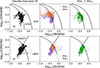 |
Fig. 13. BPT diagrams. Each dot corresponds to a MaNGA spaxel. The zones separated by the lines are named in the left column panels, with SF standing for star-forming, and comp. for composite. |
5. Discussion
Thanks to the high velocity resolution of NOEMA observations and the low velocity dispersion of molecular gas, we were able to model two discs to the system J221024.49+114247.0. The main difference between our separation into two components and the one performed by Mazzilli Ciraulo et al. (2021) is the similar rotation velocities of the two discs. While the problem is degenerate and the exact values found in this work should be taken with caution, we conclude that the rotation velocities of the discs indicate that the system is a major merger, rather than a minor merger as was found previously. This holds at least for a modelling with only two axisymmetric discs. A determination of the dynamical mass of each galaxy can only be approximate, because the radial extent of the CO(1–0) emission is limited (compared to that of atomic hydrogen HI, ideal for rotation curves) and the shape of the ‘secondary’ galaxy (disc2) is uncertain.
Decomposition of the MaNGA emission lines is more difficult for several reasons: the intrinsic velocity dispersion of the ionised gas is larger than the one of the molecular gas, the instrumental LSF is large (with a dispersion ≃70 km/s), and the removal of the stellar contribution to the spectra adds uncertainty. A fitting of a model of two discs for both the stellar contribution and the gas contribution would be even more degenerate. It is thus much more difficult to fit any disc model to the MaNGA data than to the NOEMA data. The lower rotation velocity found by Mazzilli Ciraulo et al. (2021) for the secondary galaxy (disc2) mainly comes from their assumption that the emission of spaxels best fitted by single Gaussians was from the main galaxy, likely removing some of the low-velocity region of the secondary galaxy, and also from an S/N cut on the flux of the secondary galaxy, which removed some of its high-velocity region. Resorting to statistics on the velocity distribution of the spaxels after cutting out spaxels of both low and high velocities provided a lower rotation velocity than with our modelling by a disc.
The modelling presented here, while theoretically motivated (reproducing well-defined models of rotating discs), is conceptually too simple to capture the kinematics of the system. It considers two discs without non-axisymmetries, warps, or tidal features, and hence is bound to be imperfect given the complex and perturbed optical images. The problem, because of the spatial and spectral overlap of galaxies, is already degenerate, and the size of disc2 is only a few times the size of the NOEMA synthesised beam. We thus did not aim to reproduce the whole complexity of the system by adding even more parameters (describing warps, for example), but to explore how far we could go in the understanding of the system with this two-simple-discs modelling.
Further uncertainty in the study of NOEMA observations comes from the unknown value of the conversion factor, αCO, which may differ on average from one disc to the other, and vary across each disc. A number of works show that this factor is lower in mergers (see Bolatto et al. 2013 and references therein), because of the large column densities, temperatures, and large velocity dispersions. The existence of an outflow is also possible, with, again, a different conversion factor to consider. Outflowing gas, with a lower conversion factor than gas in discs, may contribute to the central part of the total spectrum.
The depletion time of the system is large for a major merger. This may be caused by an overestimation of the molecular gas mass. The system may also be at the early stages of the merger, with no large consumption of molecular gas by merger-induced star-formation yet.
6. Conclusion
We further investigated J221024.49+114247.0, a z = 0.09228 system previously studied in Mazzilli Ciraulo et al. (2021) and Mazzilli Ciraulo et al. (2024), through interferometric NOEMA CO(1–0) observations. The high-velocity resolution of the NOEMA observations and the low-velocity dispersion of molecular gas allowed us to constrain a model of two counter-rotating discs. We aimed to make the best of this simple two-disc model without any non-axisymmetric feature in discs, for both molecular and ionised gas, while the reality is very likely more complex.
This revisited the system as being a major merger. We applied the model to the ionised-gas MaNGA emission lines and were able to draw resolved KS diagrams for both discs. The CO-to-molecular-gas conversion factor, however, remains uncertain, especially for a system of interacting galaxies.
While this system is complicated to dissect because of the degeneracy induced by the superposition on the line of sight, further observations may allow us to deepen our understanding of its physics; some resolved radio-continuum or infrared JWST observations would allow us to further study its star formation and a potential obscured AGN. Finally, such a source will be detectable in HI with SKA.
Transformations between different world coordinate systems and a significant amount of plotting in the present work were performed with astropy (Astropy Collaboration 2013).
The first two maps are the usual moments of observational studies of molecular gas, and the third one should be multiplied by  to obtain the more usually defined second moment.
The threshold value was lowered in combination with a cleaning procedure removing small groups of voxels remaining after cutting below a threshold.
Several position–velocity diagrams of this complex NOEMA cube are shown in the analyses of Sect. 4, either after integration over one spatial direction or for thin slices but after rotation of the NOEMA cube using position angles of modelled discs.
Using the gas-phase metallicity map, one may try to compute a spatial grid of conversion factors, assuming the dependency of the conversion factor on metallicity of Genzel et al. (2015), even if the latter applies to whole galaxies. Such a map is shown in the last panel of Fig. B.1. With this spatially dependent conversion factor, a molecular-gas mass very close to the one assuming a uniform conversion factor is obtained: Mmol gas = 4.1 × 10¹⁰ M⊙ (MH2 = 3.1 × 10¹⁰ M⊙).
The Hα-based SFR, computed assuming a Salpeter (1955) IMF, is divided by 1.7 for these computations in order to assume a Chabrier (2003) IMF, as used by Salim et al. (2016), Speagle et al. (2014), and Tacconi et al. (2018). The depletion time was thus multiplied by 1.7 for the comparison. This factor was obtained considering that masses of stars range from 0.1 to 100 M⊙, and assuming that only stars with masses larger than 20 M⊙ contribute to the ionisation seeding the Hα flux.
Gaussian kernels were built for the NOEMA beam and the MaNGA PSF using the radio-beam package, convolution is performed with astropy (Astropy Collaboration 2013), and reprojection with the reproject package, using a bilinear interpolation.
Acknowledgments
This work is based on observations carried out under project number S21BQ001 with the IRAM NOEMA Interferometer [30 m telescope]. IRAM is supported by INSU/CNRS (France), MPG (Germany) and IGN (Spain). We thank all the IRAM people who contributed to the observations and helped with their reduction. Funding for the Sloan Digital Sky Survey V has been provided by the Alfred P. Sloan Foundation, the Heising-Simons Foundation, the National Science Foundation, and the Participating Institutions. SDSS acknowledges support and resources from the Center for High-Performance Computing at the University of Utah. SDSS telescopes are located at Apache Point Observatory, funded by the Astrophysical Research Consortium and operated by New Mexico State University, and at Las Campanas Observatory, operated by the Carnegie Institution for Science. The SDSS web site is www.sdss.org. SDSS is managed by the Astrophysical Research Consortium for the Participating Institutions of the SDSS Collaboration, including the Carnegie Institution for Science, Chilean National Time Allocation Committee (CNTAC) ratified researchers, Caltech, the Gotham Participation Group, Harvard University, Heidelberg University, The Flatiron Institute, The Johns Hopkins University, L’Ecole polytechnique fédérale de Lausanne (EPFL), Leibniz-Institut für Astrophysik Potsdam (AIP), Max-Planck-Institut für Astronomie (MPIA Heidelberg), Max-Planck-Institut für Extraterrestrische Physik (MPE), Nanjing University, National Astronomical Observatories of China (NAOC), New Mexico State University, The Ohio State University, Pennsylvania State University, Smithsonian Astrophysical Observatory, Space Telescope Science Institute (STScI), the Stellar Astrophysics Participation Group, Universidad Nacional Autónoma de México, University of Arizona, University of Colorado Boulder, University of Illinois at Urbana-Champaign, University of Toronto, University of Utah, University of Virginia, Yale University, and Yunnan University.
References
- Astropy Collaboration (Robitaille, T. P., et al.) 2013, A&A, 558, A33 [NASA ADS] [CrossRef] [EDP Sciences] [Google Scholar]
- Baldwin, J. A., Phillips, M. M., & Terlevich, R. 1981, PASP, 93, 5 [Google Scholar]
- Bigiel, F., Leroy, A., Walter, F., et al. 2008, AJ, 136, 2846 [NASA ADS] [CrossRef] [Google Scholar]
- Bolatto, A. D., Wolfire, M., & Leroy, A. K. 2013, ARA&A, 51, 207 [CrossRef] [Google Scholar]
- Bundy, K., Bershady, M. A., Law, D. R., et al. 2015, ApJ, 798, 7 [Google Scholar]
- Chabrier, G. 2003, PASP, 115, 763 [Google Scholar]
- Chilingarian, I., Prugniel, P., Sil’Chenko, O., & Koleva, M. 2007a, in Stellar Populations as Building Blocks of Galaxies, eds. A. Vazdekis, & R. Peletier, IAU Symp., 241, 175 [NASA ADS] [Google Scholar]
- Chilingarian, I. V., Prugniel, P., Sil’Chenko, O. K., & Afanasiev, V. L. 2007b, MNRAS, 376, 1033 [NASA ADS] [CrossRef] [Google Scholar]
- Combes, F., García-Burillo, S., Audibert, A., et al. 2019, A&A, 623, A79 [NASA ADS] [CrossRef] [EDP Sciences] [Google Scholar]
- Dey, A., Schlegel, D. J., Lang, D., et al. 2019, AJ, 157, 168 [Google Scholar]
- Downes, D., & Solomon, P. M. 1998, ApJ, 507, 615 [NASA ADS] [CrossRef] [Google Scholar]
- Freundlich, J., Combes, F., Tacconi, L. J., et al. 2013, A&A, 553, A130 [NASA ADS] [CrossRef] [EDP Sciences] [Google Scholar]
- Genzel, R., Tacconi, L. J., Combes, F., et al. 2012, ApJ, 746, 69 [Google Scholar]
- Genzel, R., Tacconi, L. J., Lutz, D., et al. 2015, ApJ, 800, 20 [Google Scholar]
- Goddard, D., Thomas, D., Maraston, C., et al. 2017, MNRAS, 466, 4731 [NASA ADS] [Google Scholar]
- Gwyn, S. D. J. 2008, PASP, 120, 212 [Google Scholar]
- Hubble, E. P. 1926, ApJ, 64, 321 [Google Scholar]
- Jin, G., Dai, Y. S., Pan, H.-A., et al. 2021, ApJ, 923, 6 [NASA ADS] [CrossRef] [Google Scholar]
- Kauffmann, G., Heckman, T. M., Tremonti, C., et al. 2003, MNRAS, 346, 1055 [Google Scholar]
- Kennicutt, R. C., Jr 1998, ARA&A, 36, 189 [NASA ADS] [CrossRef] [Google Scholar]
- Kewley, L. J., Heisler, C. A., Dopita, M. A., & Lumsden, S. 2001, ApJS, 132, 37 [Google Scholar]
- Leroy, A. K., Walter, F., Brinks, E., et al. 2008, AJ, 136, 2782 [Google Scholar]
- Lin, L., Pan, H.-A., Ellison, S. L., et al. 2019, ApJ, 884, L33 [NASA ADS] [CrossRef] [Google Scholar]
- Maschmann, D., Halle, A., Melchior, A.-L., Combes, F., & Chilingarian, I. V. 2023, A&A, 670, A46 [NASA ADS] [CrossRef] [EDP Sciences] [Google Scholar]
- Maschmann, D., Melchior, A.-L., Mamon, G. A., Chilingarian, I. V., & Katkov, I. Y. 2020, A&A, 641, A171 [NASA ADS] [CrossRef] [EDP Sciences] [Google Scholar]
- Mazzilli Ciraulo, B., Melchior, A.-L., Maschmann, D., et al. 2021, A&A, 653, A47 [NASA ADS] [CrossRef] [EDP Sciences] [Google Scholar]
- Mazzilli Ciraulo, B., Melchior, A.-L., Combes, F., & Maschmann, D. 2024, A&A, 690, A143 [NASA ADS] [CrossRef] [EDP Sciences] [Google Scholar]
- Miyamoto, M., & Nagai, R. 1975, PASJ, 27, 533 [NASA ADS] [Google Scholar]
- Neumann, J., Thomas, D., Maraston, C., et al. 2022, MNRAS, 513, 5988 [NASA ADS] [Google Scholar]
- O’Donnell, J. E. 1994, ApJ, 422, 158 [Google Scholar]
- Osterbrock, D. E., & Ferland, G. J. 2006, Astrophysics of Gaseous Nebulae and Active Galactic Nuclei (Sausalito: University Science Books) [Google Scholar]
- Pettini, M., & Pagel, B. E. J. 2004, MNRAS, 348, L59 [NASA ADS] [CrossRef] [Google Scholar]
- Salim, S., Lee, J. C., Janowiecki, S., et al. 2016, ApJS, 227, 2 [NASA ADS] [CrossRef] [Google Scholar]
- Salpeter, E. E. 1955, ApJ, 121, 161 [Google Scholar]
- Schmidt, M. 1959, ApJ, 129, 243 [NASA ADS] [CrossRef] [Google Scholar]
- Solomon, P. M., Downes, D., Radford, S. J. E., & Barrett, J. W. 1997, ApJ, 478, 144 [NASA ADS] [CrossRef] [Google Scholar]
- Speagle, J. S., Steinhardt, C. L., Capak, P. L., & Silverman, J. D. 2014, ApJS, 214, 15 [Google Scholar]
- Tacconi, L. J., Genzel, R., Saintonge, A., et al. 2018, ApJ, 853, 179 [Google Scholar]
- Westfall, K. B., Cappellari, M., Bershady, M. A., et al. 2019, AJ, 158, 231 [Google Scholar]
Appendix A: Visualisation of the NOEMA cube
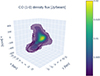 |
Fig. A.1. Visualisation of the NOEMA cube. This is a screenshot of the 3D widget of the cube made with plotly and available at https://vm-weblerma.obspm.fr/ahalle/noemacube.html |
Appendix B: Maps from MaNGA
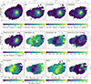 |
Fig. B.1. Maps obtained from the MaNGA data fitted by a double-Gaussian procedure. NOEMA CO(1–0) intensity contours are over-plotted in grey. The 3″ SDSS fibre is over-plotted in a dashed black circle. The elliptical aperture used to compute gas-phase metallicity is over-plotted in orange on the gas-phase metallicity map and the conversion factor map (see text). |
Appendix C: Two-disc modelling for CO(1–0)
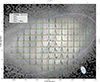 |
Fig. C.1. NOEMA CO(1–0) observations and models of two discs, superimposed on the MegaCam r-band image. NOEMA pixels encompassing the centre of the discs are shown. Fits are done on NOEMA spaxels but for the figure, NOEMA spectra and our fits are binned 16 by 16 and shown in brown boxes encompassing these binned spaxels. The velocity axis of each box is from -800 to 800 km/s. The two same ticks for values 0, on the baseline of spectra, and 0.01, are shown on the left and right y axes of each box, to show the scale which is adapted to each box. The NOEMA elliptical Gaussian synthesised beam is shown on the bottom-right. The outermost contour of NOEMA CO(1–0) intensity is shown in blue. |
Appendix D: Two-disc modelling for [OIII]
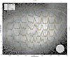 |
Fig. D.1. [OIII] 5008 Å MaNGA observations and models of two discs, superimposed on the MegaCam r-band image. MaNGA pixels encompassing the centre of the discs are shown. Fits are done on original MaNGA spaxels but for the figure, MaNGA spectra and our fits are binned 16 by 16 and shown in brown boxes encompassing these binned spaxels. The velocity axis of each box is from -800 to 800 km/s. The two same ticks for values 0, on the baseline of spectra, and 0.01, are shown on the left and right y axes of each box, to show the scale which is adapted to each box. The Gaussian reconstructed MaNGA PSF is shown on the bottom-right. The outermost contour of NOEMA CO(1–0) intensity is shown in blue. |
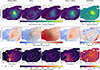 |
Fig. D.2. Observations, models and residuals of intensity, velocity and velocity dispersion from the [OIII] 5008 Å line. Models are shown both for each disc (column 2 and 3) and for the two superposed discs (column 4). Residuals are the observations (column 1) minus the two superposed discs (column 4). On the velocity maps of individual discs, iso-line-of-sight velocity curves are represented in black dashed (resp. solid) lines for values below (resp. above) the systemic velocity of the disc. |
All Tables
All Figures
|
Fig. 1. Legacy composite image (left) and log10 of MegaPipe image (right), from MegaCam on CFHT. The 3″ SDSS fibre is over-plotted with a dashed black circle. |
| In the text | |
|
Fig. 2. Intensity, velocity, and velocity dispersion obtained for CO(1–0) NOEMA observations. A flux-density threshold of 1 mJy/beam is applied. We over-plot linearly spaced contours of the CO(1–0) intensity on each map. The NOEMA elliptical, Gaussian synthesised beam is represented in the bottom left corners of the panels. The IRAM 30 m CO(1–0) and CO(2–1) beams are shown in brown and yellow, respectively. The 3″ SDSS fibre is over-plotted with a dashed black circle. |
| In the text | |
|
Fig. 4. Velocity channel maps. The 3″ SDSS fibre is over-plotted with a dashed black circle. |
| In the text | |
|
Fig. 3. NOEMA CO(1–0) spectrum stacked over a 22 arcsec aperture, compared to the IRAM 30 m spectra, at the same velocity resolution. |
| In the text | |
|
Fig. 5. Top row: molecular-gas surface density (left), Hα-based SFR surface density (middle) and stellar surface density (right). CO(1–0) intensity contours are over-plotted in grey. The 3″ SDSS fibre is over-plotted with a dashed black circle. Bottom row: diagrams obtained after degrading the maps to the same spatial resolution (see text). From left to right: KS diagram with 2D bins colour-coded by the number of contributing MaNGA spaxels; KS diagram with one dot per MaNGA spaxel, colour-coded by its distance to the centre of the SDSS fibre; molecular-gas surface density versus stellar surface density; and SFR surface density versus stellar surface density. In the two KS diagrams, locations of constant depletion times are shown as diagonal black lines, and as a diagonal blue line for the average depletion time of high-density molecular gas. |
| In the text | |
|
Fig. 6. Velocity and velocity dispersion of Hα from the Gaussian-fit procedure. |
| In the text | |
|
Fig. 7. Attempt to reconstruct the observed spectrum, assuming there are two discs, that each one has a half part accounting for the CO(1–0) emission at the lowest or highest observed velocities, and that the CO(1–0) emission of each disc is symmetric with regard to its minor kinematic axis. The violet (resp. orange) line is an example of systemic velocity for the first (resp. second) disc, with the spectrum of the disc in the same colour in the top panel. Top: NOEMA spectrum; discs’ spectra reconstructed by symmetry and their sum. Middle: NOEMA cube integrated on declination. Bottom: NOEMA cube integrated on RA. |
| In the text | |
|
Fig. 8. Position–velocity diagrams of NOEMA observations centred on estimated kinematic centre of disc1 (first row) or on the estimated kinematic centre of disc2 (second row) and computed on a one-spatial-pixel-wide slice either along the major axes (first column) or the minor axes (second column) of discs. vc(R)sin(i) curves are represented on diagrams with position taken along the major axis (first column). Horizontal solid lines show the fitted systemic velocities, vsys, of the discs, and horizontal dashed lines show vsys ± Vmaxsin(i). Violet lines correspond to disc1 and orange curves to disc2. The horizontal grey lines in the bottom right corner of each panel show the projection of the elliptical Gaussian NOEMA synthesised beam on the x-axis of the panel. |
| In the text | |
|
Fig. 9. Observation and model of CO(1–0) emission integrated on the system. Solid vertical lines show the fitted systemic velocities vsys of the discs and dashed vertical lines show vsys ± Vmaxsin(i). |
| In the text | |
|
Fig. 10. Observations, models, and residuals of intensity, velocity, and velocity dispersion from the CO(1–0) line. Models are shown both for each disc (columns 2 and 3) and for the two superposed discs (column 4). Residuals are the observation (column 1) minus the two superposed discs (column 4). On the velocity maps of individual discs, iso-line-of-sight velocity curves are represented by dashed (resp. solid) black lines for values below (resp. above) the systemic velocity of the disc. |
| In the text | |
|
Fig. 11. Observations and models of MaNGA emission lines integrated on the system. |
| In the text | |
|
Fig. 12. KS diagrams. Left: Two superposed model discs, with no correction for inclination. Middle and right: Disc1 (resp. disc2), correcting for the modelled inclinations of 60 and 65 degrees, respectively. |
| In the text | |
|
Fig. 13. BPT diagrams. Each dot corresponds to a MaNGA spaxel. The zones separated by the lines are named in the left column panels, with SF standing for star-forming, and comp. for composite. |
| In the text | |
|
Fig. A.1. Visualisation of the NOEMA cube. This is a screenshot of the 3D widget of the cube made with plotly and available at https://vm-weblerma.obspm.fr/ahalle/noemacube.html |
| In the text | |
|
Fig. B.1. Maps obtained from the MaNGA data fitted by a double-Gaussian procedure. NOEMA CO(1–0) intensity contours are over-plotted in grey. The 3″ SDSS fibre is over-plotted in a dashed black circle. The elliptical aperture used to compute gas-phase metallicity is over-plotted in orange on the gas-phase metallicity map and the conversion factor map (see text). |
| In the text | |
|
Fig. C.1. NOEMA CO(1–0) observations and models of two discs, superimposed on the MegaCam r-band image. NOEMA pixels encompassing the centre of the discs are shown. Fits are done on NOEMA spaxels but for the figure, NOEMA spectra and our fits are binned 16 by 16 and shown in brown boxes encompassing these binned spaxels. The velocity axis of each box is from -800 to 800 km/s. The two same ticks for values 0, on the baseline of spectra, and 0.01, are shown on the left and right y axes of each box, to show the scale which is adapted to each box. The NOEMA elliptical Gaussian synthesised beam is shown on the bottom-right. The outermost contour of NOEMA CO(1–0) intensity is shown in blue. |
| In the text | |
|
Fig. D.1. [OIII] 5008 Å MaNGA observations and models of two discs, superimposed on the MegaCam r-band image. MaNGA pixels encompassing the centre of the discs are shown. Fits are done on original MaNGA spaxels but for the figure, MaNGA spectra and our fits are binned 16 by 16 and shown in brown boxes encompassing these binned spaxels. The velocity axis of each box is from -800 to 800 km/s. The two same ticks for values 0, on the baseline of spectra, and 0.01, are shown on the left and right y axes of each box, to show the scale which is adapted to each box. The Gaussian reconstructed MaNGA PSF is shown on the bottom-right. The outermost contour of NOEMA CO(1–0) intensity is shown in blue. |
| In the text | |
|
Fig. D.2. Observations, models and residuals of intensity, velocity and velocity dispersion from the [OIII] 5008 Å line. Models are shown both for each disc (column 2 and 3) and for the two superposed discs (column 4). Residuals are the observations (column 1) minus the two superposed discs (column 4). On the velocity maps of individual discs, iso-line-of-sight velocity curves are represented in black dashed (resp. solid) lines for values below (resp. above) the systemic velocity of the disc. |
| In the text | |
Current usage metrics show cumulative count of Article Views (full-text article views including HTML views, PDF and ePub downloads, according to the available data) and Abstracts Views on Vision4Press platform.
Data correspond to usage on the plateform after 2015. The current usage metrics is available 48-96 hours after online publication and is updated daily on week days.
Initial download of the metrics may take a while.