| Issue |
A&A
Volume 704, December 2025
|
|
|---|---|---|
| Article Number | A55 | |
| Number of page(s) | 18 | |
| Section | Numerical methods and codes | |
| DOI | https://doi.org/10.1051/0004-6361/202556626 | |
| Published online | 03 December 2025 | |
Efficient Bayesian analysis of kilonovae and gamma ray burst afterglows with FIESTA
1
Institut für Physik und Astronomie, Universität Potsdam,
Haus 28, Karl-Liebknecht-Str. 24/25,
14476
Potsdam,
Germany
2
Institute for Gravitational and Subatomic Physics (GRASP), Utrecht University,
Princetonplein 1,
3584 CC
Utrecht,
The Netherlands
3
Nikhef,
Science Park 105,
1098 XG
Amsterdam,
The Netherlands
4
Department of Physics and Earth Science, University of Ferrara,
via Saragat 1,
44122
Ferrara,
Italy
5
INFN, Sezione di Ferrara,
via Saragat 1,
44122
Ferrara,
Italy
6
INAF, Osservatorio Astronomico d’Abruzzo,
via Mentore Maggini snc,
64100
Teramo,
Italy
7
DTU Space, National Space Institute, Technical University of Denmark,
Elektrovej 327/328,
2800
Kongens Lyngby,
Denmark
8
Max Planck Institute for Gravitational Physics (Albert Einstein Institute),
Am Mühlenberg 1,
Potsdam
14476,
Germany
★ Corresponding authors: This email address is being protected from spambots. You need JavaScript enabled to view it.
; This email address is being protected from spambots. You need JavaScript enabled to view it.
Received:
28
July
2025
Accepted:
20
October
2025
Abstract
Gamma-ray burst (GRB) afterglows and kilonovae (KNe) are electromagnetic transients that can accompany binary neutron star (BNS) mergers. Therefore, studying their emission processes is of general interest for constraining cosmological parameters or the behavior of ultra-dense matter. One common method to analyze electromagnetic data from BNS mergers is to sample a Bayesian posterior over the parameters of a physical model for the transient. However, sampling the posterior is computationally costly and because of the many likelihood evaluations required in this process, detailed models are too expensive to be used directly in Bayesian inference. In this paper, we address the problem by introducing FIESTA, a PYTHON package to train machine learning (ML) surrogates for GRB afterglow and kilonova models that have the capacity to accelerate likelihood evaluations. Specifically, we introduce extensive ML surrogates for the state-of-the-art GRB afterglow models AFTERGLOWPY and PYBLASTAFTERGLOW, along with a new surrogate for KN emission based on the POSSIS code. Our surrogates enable evaluation of the light-curve posterior within minutes. We also provide built-in posterior sampling capabilities in FIESTA that rely on the FLOWMC package, which efficiently scale to higher dimensions when adding up to tens of nuisance sampling parameters. Because of its use of the JAX framework, FIESTA also allows for GPU acceleration during both surrogate training and posterior sampling. We applied our framework to reanalyze AT2017gfo/GRB170817A and GRB211211A with our surrogates, thus employing the new PYBLASTAFTERGLOW model for the first time in Bayesian inference.
Key words: relativistic processes / methods: data analysis / gamma-ray burst: general / stars: neutron
© The Authors 2025
 Open Access article, published by EDP Sciences, under the terms of the Creative Commons Attribution License (https://creativecommons.org/licenses/by/4.0), which permits unrestricted use, distribution, and reproduction in any medium, provided the original work is properly cited.
This article is published in open access under the Subscribe to Open model. This email address is being protected from spambots. You need JavaScript enabled to view it. to support open access publication.
1 Introduction
Gamma-ray bursts (GRBs) and kilonovae (KNe) are types of electromagnetic transients that can originate from a binary neutron star (BNS) merger, as confirmed most prominently by the observation of AT2017gfo (Utsumi et al. 2017; Coulter et al. 2017; Andreoni et al. 2017; Shappee et al. 2017; Soares-Santos et al. 2017; Lipunov et al. 2017; Valenti et al. 2017; Díaz et al. 2017; Tanvir et al. 2017) and GRB170817A (Goldstein et al. 2017; Abbott et al. 2017b; Savchenko et al. 2017) in the wake of the gravitational wave (GW) event GW170817 (Abbott et al. 2017c,d). Additionally, several GRBs have been associated with potential subsequent KNe (Tanvir et al. 2013; Ascenzi et al. 2019; Troja et al. 2019b; Rastinejad et al. 2022; Troja et al. 2018; Levan et al. 2024; Yang et al. 2024; Levan et al. 2023; Stratta et al. 2025). To analyze these electromagnetic transients with Bayesian inference, a physical model that links the source and observational parameters of the system (e.g., ejecta masses, isotropic energy equivalent of the jet, observation angle) to the observed data is needed. This model can then be employed in a sampling procedure to obtain a posterior distribution.
The KN emission arises from quasi-thermal radiation produced by the BNS ejecta heated from the radioactive decay of nuclei synthesized through the r-process (Thielemann et al. 2011) and is observed on the timescale of days after the merger. This process has been investigated through various methods and approaches in the literature (e.g., Kasen et al. 2017; Villar et al. 2017; Kawaguchi et al. 2018; Metzger 2020; Breschi et al. 2021; Wollaeger et al. 2021; Curtis et al. 2022; Nicholl et al. 2021; Bulla 2023). The GRB prompt emission, on the other hand, takes place on scales of seconds to minutes and is observed as bursts of highly energetic gamma and X-ray radiation. Its emission mechanism is largely uncertain and, thus, the associated data are typically not taken into account for Bayesian inference of BNS mergers. However, the prompt emission is followed by an afterglow of broadband radiation spanning from radio to γ-ray frequencies, observable on timescales ranging from minutes to years (Miceli & Nava 2022). Unlike the GRB prompt emission, the afterglow physics are comparatively well understood and can thus be used to infer properties of the jet and the progenitor. Specifically, the afterglow emission arises from the interaction of the GRB jet with the surrounding cold interstellar medium and various afterglow models are available in the literature (e.g., van Eerten et al. 2012; Ryan et al. 2015; Lamb et al. 2018; Ryan et al. 2020; Zhang et al. 2021; Pellouin & Daigne 2024; Wang et al. 2024; Nedora et al. 2025; Wang et al. 2026).
Such models have been successfully applied in joint Bayesian analysis of GW170817, its KN, and the GRB afterglow to place constraints on the equation of state (EOS) for neutron star (NS) matter (Radice et al. 2018b; Dietrich et al. 2020; Raaijmakers et al. 2021; Nicholl et al. 2021; Pang et al. 2023; Güven et al. 2020; Annala et al. 2022; Breschi et al. 2024; Koehn et al. 2025) or to determine the Hubble constant (Abbott et al. 2017a; Hotokezaka et al. 2019; Dietrich et al. 2020; Mukherjee et al. 2021; Wang & Giannios 2021; Gianfagna et al. 2024). However, these joint multi-messenger inferences pose certain computational challenges, because exploring their high-dimensional parameter space requires many likelihood evaluations. Therefore, a single likelihood evaluation needs to be as cheap as possible in order to keep the total sampling time manageable. However, to evaluate the likelihood function at a given parameter point, we have to determine the expected emission for these given parameters from the physical model. Due to the cost limit on the likelihood function, any direct, physical calculation of the emission on-the-fly is only viable with computationally cheap, semi-analytical models. Yet, even relatively efficient models can become prohibitive, when considering multi-messenger inferences of BNS mergers signals, where GW and electromagnetic signals are analyzed jointly in a large parameter space. Accordingly, applying more expensive and involved models in multi-messenger inference necessitates the development of accurate surrogate models, often through machine learning (ML) techniques to enable likelihood evaluation at sufficient speeds (Pang et al. 2023; Almualla et al. 2021; Kedia et al. 2023; Ristic et al. 2022; Boersma & van Leeuwen 2023). Furthermore, joint multi-messenger BNS inferences also provide motivation for the GPU compatible light-curve surrogates, since the analysis of BNS GW data can be significantly accelerated on GPU hardware (Wysocki et al. 2019; Wouters et al. 2024; Hu et al. 2025; Dax et al. 2025).
In the present article, we introduce FIESTA, a JAX-based PYTHON package for training ML surrogates of KN and GRB afterglow models and for the Bayesian analysis of photometric transient light curves. With FIESTA, we provide extensive ML surrogates that effectively replace the costly evaluation of the physical base model, enabling rapid prediction of the expected light curve given the model’s parameters. Specifically, we present surrogates that are built upon GRB afterglow models from the popular AFTERGLOWPY model (Ryan et al. 2020) and the recently developed PYBLASTAFTERGLOW (Nedora et al. 2025). Additionally, we introduce a new KN surrogate based on the 3D Monte Carlo radiation transport code POSSIS (Bulla 2019, 2023). In contrast to many previous works, our surrogates have not been trained on the magnitudes in a specific photometric passband; instead, they predict the entire spectral flux density, providing maximal flexibility. Given photometric transient data, FIESTA’S surrogates can be used in stochastic samplers to achieve fast evaluation of the likelihood, which opens the door for swift transient analysis. Such analyses can be conducted using the established inference framework NMMA (Pang et al. 2023), which our surrogates are compatible with. In addition, FIESTA also contains its own sampling implementation that relies on the FLOWMC package (Wong et al. 2023a) to generate the posterior Markov chain Monte Carlo (MCMC) chain with normalizing flows and the Metropolis-adjusted Langevin algorithm (MALA). These advanced sampling techniques reduce the number of likelihood evaluations needed and thus sample the posterior more efficiently, thereby improving the scaling of FIESTA as we consider additional nuisance parameters to account for systematic uncertainties. Because FIESTA uses the JAX framework, surrogate training as well as posterior sampling can be GPU-accelerated.
The approach implemented in FIESTA enables sampling the full light-curve posterior within minutes, which, depending on the base model, would previously have either taken several hours to days or proven prohibitively expensive from the start. Therefore, the FIESTA surrogates make previously intractable models available for Bayesian inference, which allows us to present the first Bayesian analyses of GRB afterglows with PYBLASTAFTER-GLOW. The FIESTA code together with the surrogates is publicly available1 and all the data used in the present article can be accessed as well2.
The present article is organized as follows: in Sect. 2, we briefly review Bayesian inference of photometric transient data. We then continue in Sect. 3 discussing machine learning approaches to create surrogate models for the KN and GRB afterglow emission and present our flagship surrogates for AFTER-GLOWPY, PYBLASTAFTERGLOW, and POSSIS. From there, we verify that our surrogates are able to accurately recover the posterior and discuss their performance in Sect. 4. In Sect. 5, we apply FIESTA to analyze the data from AT2017gfo/GRB170817A and GRB211211A before concluding in Sect. 6. Throughout, we use the AB magnitude system to convert interchangeably between flux densities, Fν, and magnitudes,
 (1)
(1)
where e(ν) is the detector response function. In this way, even X-ray or radio flux density measurements can be expressed as magnitudes within FIESTA.
2 Bayesian inference of transients
Given some photometric light curve data d, the goal is to find the posterior P(θ|d), where θ denotes the parameters of the model that describes the physical emission process. The posterior can be obtained by using Bayes’ theorem,
 (2)
(2)
where L(θ|d) is called the likelihood function, π(θ) the prior distribution, and Z is the Bayesian evidence. The latter is an important quantity for model selection (e.g., jet geometries in the context of GRBs). Since the posterior is often analytically intractable, stochastic sampling methods are used. One technique is nested sampling (Skilling 2004, 2006), which computes the Bayesian evidence (i.e., the normalization constant of the posterior distribution, see Eq. (2)), from which posterior samples can be obtained as a byproduct. Alternatively, we can look to MCMC methods (Neal 2011), which directly generate samples from the posterior. Direct MCMC methods can only provide an estimate of the evidence if they are supplemented with additional techniques such as parallel tempering (Marinari & Parisi 1992) or the learned harmonic mean estimator (Newton & Raftery 1994; McEwen et al. 2023; Polanska et al. 2025). However, we do not consider these approaches in the present article.
In the context of photometric light curve analyses, we denote the observed data, d, as a time series of magnitudes {m(tj)| j = 1,2,3 ...}, and the corresponding predictions of the model as m*(tj,θ). The data are taken with some measurement uncertainty, σ(tj). In FIESTA, we assume that this uncertainty is Gaussian and hence the corresponding likelihood function can be written as
 (3)
(3)
Here, σsys(tj) is the model systematic uncertainty that accounts for both the surrogate error and the systematic offset caused by simplifying assumptions in the physical base model. Moreover, detection limits can also be incorporated into FIESTA’S likelihood. For every detection limit m▼ (tj), the likelihood in Eq. (3) is simply multiplied by
 (4)
(4)
We note that depending on the detector and measurement, other likelihood statistics might be more appropriate. For instance, for low-flux X-ray data, the Poisson distribution is generally better suited to describe the measurement uncertainty (Ryan et al. 2024; Humphrey et al. 2009). In FIESTA, we stick to a Gaussian likelihood and assume equal upper and lower error bars.
Existing inference frameworks such as NMMA (Pang et al. 2023), BAJES (Breschi et al. 2024), REDBACK (Sarin et al. 2024), or MOSFIT (Guillochon et al. 2018) evaluate a model or a surrogate to determine the value of Eq. (3). They either use nested sampling or MCMC methods to sample the posterior. FIESTA provides surrogates that can be used with NMMA and potentially other inference frameworks, but also contains its own sampling implementation based on the FLOWM C sampler (Wong et al. 2023a). While NMMA relies on nested sampling through the PYMULTINEST (Feroz et al. 2009) and DYNESTY (Speagle 2020) packages, FIESTA has sampling functionalities that utilize FLOWMC. The latter is an MCMC sampler enhanced by gradient-based sampling (in particular, the Metropolis-adjusted Langevin algorithm (Grenander & Miller 1994)) and normalizing flows, which are a class of generative ML methods that act as neural density estimators (Rezende & Mohamed 2015; Papamakarios et al. 2021; Kobyzev et al. 2020). The flows are trained on the fly from the MCMC chains and subsequently used as proposal distributions in an adaptive MCMC algorithm (Gabrié et al. 2022).
In both FIESTA and NMMA, the systematic error σsys(t) in Eq. (3) can either be fixed to a constant value or be sampled freely from a prior. Moreover, FIESTA and NMMA support time-and filter-dependent systematic uncertainties by sampling the nuisance parameters  at specific time nodes tk. The systematic error for a filter, f, at a specific data point, tj, is then determined via a linear interpolation,
 (5)
(5)
which is then placed into Eq. (3). The nuisance parameters,  , can be sampled separately for different filters. This implementation for a data-driven inference of the systematic uncertainty essentially follows Jhawar et al. (2025).
3 Surrogate training
To evaluate the likelihood function in Eq. (3) efficiently, FIESTA provides surrogates that determine the expected magnitudes, m*(tj,θ ), for a given parameter point θ through ML surrogates. For KN models, previous works have demonstrated the capability of ML techniques to replace the expensive light curve generation of radiative transfer models, which enabled their use in stochastic samplers (Almualla et al. 2021; Ristic et al. 2022; Kedia et al. 2023; Lukosiüte et al. 2022; Ristic et al. 2023; Ford et al. 2024; Saha et al. 2024; King et al. 2025). For GRB afterglows, many fast semi-analytic models are available, so the use of ML surrogates has not been as essential; however, an increasing number of recent works have introduced ML techniques to this area. In Lin et al. (2021), the authors linearly interpolated a fixed table of GRB afterglow light curves from the prescription in Lamb et al. (2018) to accelerate the likelihood evaluation, although the interstellar medium density and other microphysical parameters were kept fixed. A surrogate model for the X-ray emission in AFTERGLOWPY was trained in Sarin et al. (2021) to analyze the Chandra transient CDF-S XT1. In Boersma & van Leeuwen (2023), DEEPGLOW was introduced, a PYTHON package that emulates BOXFIT (van Eerten et al. 2012) light curves through a neural network (NN). In Wallace & Sarin (2025), the authors trained an NN for the afterglow model of Lamb et al. (2018). Rinaldi et al. (2024) suggested developing an ML surrogate based on the afterglow model developed in Warren et al. (2022), but postponed the implementation to future work. In Aksulu et al. (2020, 2022), the authors used Gaussian processes to model the likelihood function in Bayesian analysis, although the expected light curves were computed directly with SCALEFIT (Ryan et al. 2015).
In the present work, we introduce the first large-scale surrogates for the state-of-the-art afterglow models AFTERGLOWPY and PYBLASTAFTERGLOW, covering the radio to hard X-ray emission over a timespan of 10−4 - 2 × 10³ days. Additionally, we extend the work of Almualla et al. (2021); Anand et al. (2023) and train a new KN surrogate with an updated version of the POSSIS code. Our surrogates provide a large speed-up, since the POSSIS Monte Carlo radiative transfer code (Bulla 2019, 2023) takes on the order of ∼1000 CPU-hours to predict a light curve. Likewise, depending on the settings, a GRB afterglow simulation in AFTERGLOWPY takes on the order of 0.1-10 seconds; whereas for PYBLASTAFTERGLOW, the computation time may exceed several minutes. In the following subsections, we provide details about the implemented ML approaches in FIESTA and present the surrogates we obtained for the GRB afterglow and KN models.
3.1 Surrogate types and architectures
To create a surrogate for FIESTA, a NN learns the relationship between the input θ, i.e., the parameters of the model, and the output y (i.e., the flux). The surrogate models thus interpolate a precomputed training data set that consists of many evaluations of the physical base model (e.g., POSSIS or PYBLASTAFTER-GLOW) on various combinations of input parameters.
Specifically, the output y could either represent the magnitudes in predefined frequency filters, or yield the spectral flux density Fν across a continuum of frequencies. In previous works, surrogate models typically predicted magnitudes for a set of predefined filters with fixed wavelength (Almualla et al. 2021; Pang et al. 2023; Peng et al. 2024). Training on the spectral flux densities provides more flexibility, as the surrogate does not need to be retrained if a new filter becomes available, and the surrogate’s output can be further processed to account for arbitrary redshifts or extinction effects. Surrogates trained on Fν will thus return a 2D-array containing the flux density across time along one dimension, and across frequency along the other dimension. FIESTA implements both types of surrogates, which we refer to as FLUXMODEL class for the latter kind of surrogate, whereas the surrogates that are trained in the traditional approach on passband magnitudes are referred to as the LIGHTCURVEMODEL class.
Regardless of the particular type of surrogate model, FIESTA employs two kinds of NN architectures, namely the simple feed-forward multilayer perceptron (MLP) and the conditional variational autoencoder (cVAE). The feed-forward NN, in this work containing three hidden layers, is used to train the relationship between the input parameters θ and the coefficients c of the principal component analysis (PCA) of the training data. The training simply minimizes the mean squared error on the PCA coefficients as loss function,
 (6)
(6)
where φ are the NN weights,  are the PCA coefficients of the training data y, and
  are the coefficients the NN would predict. The passband magnitude or flux density y is then determined by applying the inverse PCA decomposition to c. The feed-forward architecture is thus used both for LIGHTCURVEMODEL and FLUXMODEL surrogates.
The other implemented architecture is the cVAE (Kingma & Welling 2013; Rezende et al. 2014). This approach is inspired by Lukošiūte et al. (2022), where cVAEs were used to predict KN spectra. In contrast to their work, our setup predicts the flux density across a fixed grid of times and frequencies, and thus time is not a training parameter. Moreover, we extended this approach to GRB afterglows.
In the cVAE architecture, an encoder and decoder are trained simultaneously on the spectral flux densities directly. The encoder takes the parameters θ and the flux y as inputs and maps them to the latent parameters μ and σ. These parameters represent the variational distribution of the latent space from which the decoder reconstructs y. Specifically, the latent vector is drawn according to z ~ N(μ, diag(σ)) and serves as input to the decoder, together with θ. The encoder and decoder are trained on minimizing the joint loss function,
 (7)
(7)
where φ represents the NN weights, σj, μj, and  are the predicted parameters for the variational distribution and the flux, and
  is the training data. The first term in Eq. (7) represents the Kullback-Leibler divergence between the variational distribution and the standard normal distribution, while the second term is the reconstruction loss. Since the decoder is conditioned with the parameters θ, its output after training will not depend much on the latent vector, and for the actual flux prediction we set z = (0,..., 0). Since the cVAE is computationally more expensive to train, it was only implemented for FLUXMODEL surrogates, where just a single surrogate is trained, in contrast to the LIGHTCURVEMODEL where each photometric filter constitutes its own surrogate. All NNs were implemented through the FLAX API (Heek et al. 2024).
3.2 GRB afterglow surrogates
In FIESTA, we include surrogates for the GRB afterglow models AFTERGLOWPY (Ryan et al. 2020) and PYBLASTAFTER-GLOW (Nedora et al. 2025). Table 1 shows the parameter ranges and trained architectures for these models. We note that these surrogates are specific to a structured Gaussian jet. While we also created surrogates for the tophat jet models, their relevance in real-life applications is limited (Ryan et al. 2020; Salafia & Ghirlanda 2022) and we discuss their performance in Appendix A. We simply note here that the tophat jet surrogates generally outperform the surrogates for the Gaussian jet in terms of accuracy due to their simpler physical behavior.
Both AFTERGLOWPY and PYBLASTAFTERGLOW assume that the jet of the GRB can be modeled as a relativistic fluid shell that propagates trough a cold, ambient interstellar medium with constant density nism as a shockwave. The shock jumping conditions can then be used to determine the shell dynamics analytically given the initial kinetic energy E0 and bulk Lorentz factor Γ0 (Nava et al. 2013; Ryan et al. 2020). All AFTERGLOWPY and the PYBLASTAFTERGLOW runs in the present work ignore reverse shock contributions and only include the forward shock. If the jet has a Gaussian structure, then the jet is evolved as a collection of individual, independent, annular shells each of them assigned an energy according to
 (8)
(8)
where θ is the polar angle from the jet’s center axis and θc the core angle parameter of the jet. The wing angle θw is parameterized in Table 1 through the factor  . Once the dynamics have been determined, the emission is modeled as synchrotron radiation from the electrons accelerated at the shock front, which receive a fraction εe of the shock energy. The magnetic field in the downstream shock is given through a fraction εB of the shock energy. While employing a similar semi-analytical framework, AFTERGLOWPY and PYBLASTAFTERGLOW have notable differences in their specific implementation. Most notably, AFTERGLOWPY assumes that the electron distribution follows a broken power law in which newly shocked electrons are injected with
  , where p is the electron power index. PYBLASTAFTERGLOW assumes the same power law for the newly shocked electrons, but instead numerically evolves the existing electron distribution. Further differences regard the implementation of the jet spreading and initial coasting phase and the methods used to compute the synchrotron radiation spectra.
For both GRB afterglow models, we trained two surrogates of the FLUXMODEL type: one with an MLP architecture and the other with the cVAE architecture. Each surrogate was trained with input parameters as listed in Table 1. The training data was randomly drawn from the ranges specified there. The training data set for the AFTERGLOWPY Gaussian jet surrogate encompasses ntrain = 80000 flux density calculations, the set for the PYBLASTAFTERGLOW surrogate ntrain = 91 670. The surrogates were trained on standardized ln(Fν), and standardized parameter samples θ. After different attempts with similar results, the number of PCA coefficients for the MLP training was set to 50 and the cVAE trained on a down-sampled flux density array of size 42 × 57. On a H100 GPU, training took about 2.2 h for the cVAE and 0.3 h for the MLP architecture.
We used two different metrics to compare the light curves mpred(t) predicted by the surrogate against a set of test light curves mtest(t). These test light curves are from the physical base model and were not part of the training set. The one metric is the mean squared error MSE,
 (9)
(9)
and the other is the mismatch MIS,
 (10)
(10)
In Fig. 1, we show the performance of the surrogates for the AFTERGLOWPY Gaussian jet model when trying to predict the magnitudes in different passbands. Overall, the squared error is confined to <0.1 mag across different photometric filters and does not vary notably between the MLP or cVAE architectures. The panels on the right hand-side show the distribution of the absolute mismatch over time. While this mismatch is mostly within 0.3 mag, some outlier predictions show stronger deviations from the test data. Specifically, for the cVAE architecture, ∼6% of all test data samples exceed a mismatch of 1 mag at some point along the test light curve.
In Fig. 2, we show the performance of the corresponding PYBLASTAFTERGLOW surrogates for the Gaussian jet. The deviation from the test data set is typically larger than for the AFTERGLOWPY surrogate, which we attribute to higher variability in the training data arising from the additional features of PYBLASTAFTERGLOW. This is also represented in the mismatch, which typically falls in the range of <0.4 mag, though for ∼10% of the test data samples the mismatch exceeds 1 mag at least once along the light curve. We also note that the X-ray filter in the bottom right panel shows somewhat higher mismatches from the predictions. This is due to the fact that we cropped the training data below 2 · 10−22 mJys at 10 pc (corresponding roughly to the 70th absolute magnitude) due to numerical noise in the PYBLASTAFTERGLOW flux computation at very low brightness. This cutoff mostly affects the high frequencies, and since the surrogates struggle to reproduce this hard cut, the typical mismatch in the X-ray filter is higher than for the lower frequency filters. As this concerns only light curves far below the detection limit, this is no issue in real-life applications.
The MLP and cVAE architectures perform very similarly for the GRB afterglow surrogates, though the cVAEs tend to have a slightly smaller absolute mismatch in the light curve at later times. This is especially true for the PYBLASTAFTERGLOW model. Overall, the cVAEs also tend to have the smaller average square error as shown by the distributions in the left panels of Figs. 1 and 2. For these reasons, we set the cVAE as the default architecture to be used for the analyses later in Sects. 4 and 5.
Overview of FIESTA surrogates for different models.
3.3 KN surrogates
FIESTA includes surrogates for the KN model from the POSSIS code (Bulla 2019, 2023). POSSIS is a 3D Monte Carlo radiation transport code that assumes homologously expanding ejecta and determines the emitted flux and polarization at each timestep from the Monte Carlo propagation of photon packets. As the photon packets move through the matter cells in the ejecta profile, they can interact with the matter through bound-bound and electron-scattering transitions, where the prescriptions take into account temperature-, density-, and electron-fraction dependent opacities (Tanaka et al. 2020). The BNS ejecta are assumed to follow a certain geometry inspired by numerical relativity simulations (Kiuchi et al. 2017; Radice et al. 2018a; Kawaguchi et al. 2020; Hotokezaka et al. 2019). In particular, the ejecta have two components, the dynamical ejecta with mass mej,dyn and the wind ejecta with mass mej,wind. The velocity in the dynamical component ranges from 0.1 c to a cutoff value that is determined such that the mass-averaged velocity is ῡej,dyn. Likewise, the wind component has the mass-averaged velocity ῡej,wind with a minimum velocity of at least 0.02c. The dynamical electron fraction varies with the polar angle θ according to
 (11)
(11)
where a = 0.71 b (Setzer et al. 2023) and b is scaled to achieve the desired mass-averaged electron fraction Ȳe,dyn. This setup was also used in Anand et al. (2023); Ahumada et al. (2025). The electron fraction for the wind ejecta, however, is assumed to be constant and thus we do not mark its symbol Ye,wind with a bar.
We trained three POSSIS surrogates, two as a FLUXMODEL with an MLP and cVAE architecture, respectively, and the other as a LIGHTCURVEMODEL. These surrogates constitute an update for the BU2019 surrogate implemented in NMMA that was based on an older POSSIS version. Our training data consists of ntraIn = 17 899 flux densities calculated from POSSIS. For each of these computations we set the number of Monte Carlo photon packets to 107. Parameters for the training data set are randomly drawn within the ranges from Table 1, though we note that the ejecta masses were uniformly in linear space, not in log-space. Furthermore, the inclination, ι, is confined to a fixed grid from the POSSIS output that is spaced uniformly in cos(ι) between 0 (edge-on) and 1 (face-on). We also mention that the LIGHTCURVEMODEL additionally receives the redshift z sampled randomly between 0 and 0.5 as a training parameter (the luminosity distance is fixed at 10 pc), so that the surrogate automatically incorporates the K-correction to the passband magnitudes. We find no significant performance difference for various hyperparameter settings, so the final number of PCA coefficients for the MLP architecture in the FLUXMODEL and LIGHTCURVEMODEL was set to 100, the cVAE was trained on a down-sampled flux array of dimensions 64 × 40. Training took about 4 minutes for the MLP architectures and 27 minutes for the cVAE on an H100 GPU.
In Fig. 3, we benchmark the surrogate models for the POSSIS KN model. In particular, we compare the MLP FLUXMODEL against the MLP LIGHTCURVEMODEL, since the FLUXMODEL with the cVAE architecture underperforms both. This is because, in contrast to the GRB afterglow training data, the training data from POSSIS contains inherent Monte Carlo noise, which is more difficult for the cVAE to “average out”, as it is trained directly on the flux output. The MLP architecture uses the coefficients of the principal components as training input and, thus, it is less sensitive to small noise fluctuations. Still, even for those architectures, we generally find higher deviations in the predictions from the test data set than for the afterglow surrogates. In particular, the mismatch rises drastically above 0.5 mag for many test data samples when the flux brightness suddenly drops. This can be seen in Fig. 3, where the mismatch in the right panels is typically confined to <0.5 mag, but then spikes around the time the KN starts to fade (i.e., after around 1 day) in the UV band and after around > 10 days in the i-band. In general, the dimmer the light curve, the higher the Monte Carlo noise contribution and the larger the mismatch between the surrogate and the test data becomes. However, inspection of random test samples reveals that the surrogate prediction matches quite well at early times, when the absolute magnitude is still brighter than −10 mag. At very late times, we truncated the training data below 106.5 mJys (corresponding roughly to the 0th absolute magnitude), which causes the mismatch to decrease again when the surrogates pick up on this trend. The LIGHTCURVEMODEL performs slightly better at these later times, however, the FLUXMODEL performs better at earlier times when the emission is still bright. We thus set the MLP FLUXMODEL as the default KN surrogate for the subsequent analyses in Sects. 4 and 5, as the early and bright parts of the light curve are most relevant for real-life applications.
While we generally find that the surrogates presented here are well trained, the typical prediction error still exceeds the observation accuracy σ of most GRB afterglow or KN observations. However, the similar performance across the different architectures, as well as consistent performance across training runs with different hyperparameters indicates that improving the surrogates further might be challenging. Thus, when fitting to light curve data, we need to offset this surrogate error through the systematic uncertainty in the likelihood in Eq. (3).
We also note that the surrogates from Table 1 are rather extensive in their scope in which they can predict the spectral flux density. Specifically, the GRB afterglow surrogates have been trained across 109−5 · 1019 Hz, i.e., from the radio to hard X-ray, and over a time interval of 10−4−2000 days. The KN surrogates can predict the expected emission between 0.2 and 26 days in the frequency range of 1014−2 · 1015 Hz, i.e., from the far infrared to the far ultraviolet (UV). In certain use cases, the surrogates could easily be retrained on a smaller frequency or time interval, to potentially deliver even better performance.
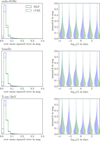 |
Fig. 1 Benchmarks of the two surrogates for the AFTERGLOWPY Gaussian jet model. We show the error distributions of the surrogate predictions against a test data set of size ntest = 7500. The different rows show the error across different passbands. The left panels show the distribution of the mean squared error as defined in Eq. (9). The right panels show the mismatch distribution across the test data set as defined in Eq. (10). The figure compares two different surrogates: one using the MLP architecture (blue) and the other a cVAE (green). |
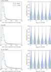 |
Fig. 2 Benchmarks of the two surrogates for the PYBLASTAFTERGLOW Gaussian jet model. We show the deviations of surrogate predictions against a test data set of size ntest = 7232. Figure layout is the same as in Fig. 1. |
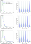 |
Fig. 3 Benchmarks of two surrogates for the KN POSSIS model. We show the deviations of surrogate predictions against a test data set of size ntest = 2238. Figure layout as in Fig. 1. The figure compares two different surrogates: one using the MLP architecture (blue) and the other a LIGHTCURVEMODEL, where an MLP is trained for each passband separately (green). |
4 Bayesian inference with fiesta
Using the surrogate for the determination of the expected light curve m*(t, θ) in Eq. (3) is an approximation to the real likelihood function. In this section, we demonstrate that this approximation is still capable of recovering the correct posterior when accounting for the surrogate uncertainty. We do so by using the best-performing surrogates presented in Sect. 3, namely, the FLUXMODEL instances with cVAE architecture for the afterglow models, and the FLUXMODEL with the MLP architecture for the KN model. We also discuss the performance of the FLOWMC implementation in FIESTA and how it scales when the dimension of the parameter space is increased to include more systematic nuisance parameters in the sampling.
4.1 Injection recoveries
To evaluate whether FIESTA’S surrogates are capable of recovering the correct posterior, we created mock light curve data with the physical base model using randomly drawn model parameters. We were then able to obtain the posterior using the surrogate. The injection data always contain 75 mock magnitude measurements across multiple bands, encompassing the frequency and time range of the model and representing a well-sampled light curve. Specifically, for GRB afterglows, the injection data span from 0.01 to 200 days and contains mock observations from the radio to the x-ray bands. The KN injections reach from the infrared to uV and contain data points between 0.5 and 20 days. For the KN injections, we also apply a detection limit of 24 apparent mag at 40 Mpc, which prevents the surrogates of being used in regions with high prediction error due to high Monte Carlo noise in the POSSIS training data. We add Gaussian noise to these mock measurements, where the measurement errors σ(tj) are drawn from a χ2−distribution with one degree of freedom and scaled to lie around 0.1 mag. To recover the posterior with the surrogate, we use uniform priors across the parameter ranges specified in Table 1. The luminosity distance is fixed to 40 Mpc for each injection.
In Fig. 4, we show how the parameters of one particular injection from the AFTERGLOWPY Gaussian jet model are recovered with FIESTA’S surrogates, using either PYMULTINEST in NMMA or FLOWMC as sampler. Since the injection also incorporates a random mock measurement error, the posterior is not always centered around the true injected parameters indicated by the orange lines, but the marginalized posteriors contain the injected values in the 95% credible interval.
Of all the models presented in Sects. 3.2 and 3.3, AFTERGLOWPY is the only one where the execution time of a single likelihood call is sufficiently fast to be used directly in Bayesian inference. Thus, we can compare the approximate posterior obtained with the FIESTA surrogate to the posterior obtained using the actual physical base model for the likelihood evaluation. The latter is shown in red in Fig. 4. We find good agreement with the posteriors obtained with the FIESTA surrogate, though some small deviations in the posterior tails for the inclination and jet opening angle exist.
We also ran four additional AFTERGLOWPY injection recoveries (similar to those in Fig. 4) and compared them to the surrogate posteriors, finding good agreement. For certain degenerate parameters, we observed that even the FLOWMC sampling algorithm with the surrogate recovers the true injected values better; namely, the true value lies more at the center of the posterior than with NMMA’s PYMULTINEST sampler and when using the actual AFTERGLOWPY model for the likelihood. This can be attributed to broader exploration in the parameter space for degenerate parameters such as εB and log10(nism), indicating an advantage in FLOWMC’s dependence on gradient-based samplers and global proposals.
To systematically evaluate the disagreement between the posteriors caused by the surrogates, we resorted to the Kullback-Leibler (KL) divergence DKL. Bevins et al. (2025) assessed a theoretical link between the root mean square error (RMSE) of an emulator and the impact on the posterior in terms of DKL if it was obtained with the base model or with the surrogate. For a linear model, they derive the upper-bound on DKL,
 (12)
(12)
where Nd is the number of data points and σ their typical error scale. While this upper bound assumes a linear relation d(θ), we can still examine this relationship using our AFTERGLOWPY injections and the respective surrogate and base model posteriors. We then determine DKL between the posteriors through a kernel density estimate. Using our 5 injection-recoveries with Nd = 75, we find that DKL ranges between 2 and 8 nats and the upper limit is indeed obeyed when setting RMSE = 0.1 mag and taking the largest error from the injected mock data as a conservative value for σ. In fact, Eq. (12) is a factor of 1.4-2.8 above our estimated value for DKL. It should be noted however, that this only serves as a limited sanity check, since the bound in Eq. (12) is derived under simplifying assumptions, and determining DKL through kernel density estimates might not be numerically accurate.
We also point out that in order to achieve this agreement between the surrogate posterior and the posterior based on AFTERGLOWPY directly, we set a minimum threshold on the systematic uncertainty σsys. Specifically, σsys was sampled as a free parameter with a uniform prior σsys ∼ U(0.3,1). Lowering the limit on σsys can lead to biases in the posteriors recovered with the surrogate, since sampling the systematic uncertainty mainly accounts for potential tension between model and data, but inherent surrogate errors need to be incorporated a priori. When we set σsys = 0, i.e., turn off the systematic uncertainty entirely, we observe that the posteriors using the surrogate diverge from the posteriors using the direct AFTERGLOWPY evaluations. Although the surrogate posteriors still find values that are close the injection parameters, the latter are not contained in the 95% credible limits. Likewise, the credibility contours between the surrogate and direct AFTERGLOWPY posterior do not overlap anymore. Thus, adjusting for the surrogate uncertainty remains crucial.
In Appendix B, we show similar injection recoveries for the PYBLASTAFTERGLOW and POSSIS surrogates. For these models, we could not compare the FIESTA posterior to a posterior that evaluates the likelihood with the physical base model, yet we still found a good recovery of the injected parameters.
However, a systematic assessment of whether injections are generally well recovered requires going beyond individual examples. For this reason, we ran 200 injection recoveries each for AFTERGLOWPY, PYBLASTAFTERGLOW, and POSSIS. This way, we obtained the distribution of the injection values’ posterior quantiles across multiple inferences. The cumulative distribution of these quantiles can be visualized in a P-P plot. Figure 5 shows the resulting P-P plot for the GRB afterglow inferences, in Fig. 6 we provide the P-P plot for the POSSIS injection recoveries. Overall, we find that the injection values are recovered well, with the injected values lying within the posterior samples in 98.7% of the AFTERGLOWPY and PYBLASTAFTERGLOW injections and in 94.8% the POSSIS injections. However, if the posteriors were unbiased, then, according to the probability integral transform, the quantiles would adhere to a uniform distribution. In Figs. 5 and 6, it is apparent that this is not always the case and the cumulative distributions sometimes fall outside the grey 68, 95, or 99.7% confidence ranges in which they would lie if they were uniform.
There are several reasons for this behavior. In certain cases, the surrogate error might introduce biases in the recovery. However, in Figs. 5 and 6 we also show P-P plots for cases where the injection data is generated with the surrogate instead of the base model. These are shown as dashed lines in Figs. 5 and 6 and display the same trends as the P-P plots with the injections from the base model. Hence, we conclude that the suboptimal recovery of certain parameters is primarily due to our inclusion of the systematic uncertainty and the way we generate the mock data.
For the GRB afterglow injection recoveries, it is the wing angle αw, the interstellar density log10(nism), and the electron power index p that show the most notable deviation from uniformity. In the case of αw, for instance, we note a high degeneracy with the output data. The light curve does not change noticeably when αw goes from 2.5 to 3.5, unless perhaps the alignment with the observer changes, i.e., θw suddenly becomes larger than ι. This leads to broad posterior support for αw, therefore causing the more extreme quantiles for αw to be overrepresented in the P-P plot. This also applies to log10(nism), which mostly affects the early part of the light curve prior to the jet-break. When log10(nism) is low, this late part of the light curve will also match a jet with somewhat higher interstellar density and the posterior will have significant support above the injected value, overrepresenting low quantiles. Our mock injection data are spaced log-uniformly from 0.01 to 200 days and thus in most cases will contain a large data segment from the post-jet break which may cause a degeneracy in log10(nism). On the other hand, for the electron power index p, the injection value’s posterior quantile is too often too close to 0.5, i.e., p is overdetermined. This can be attributed to the fact that the value for p strongly influences the post-jet break slope from the data. The large segment of postjet break data enables the sampler to infer p with good accuracy, but the addition of the systematic uncertainty artificially broadens the posterior, which causes the injected value to lie too often at the center of the posterior.
A similar effect can be seen for some of the KN parameters in Fig. 6. The parameters  ,
,  , and
, and  show the same over-determination, i.e., their quantiles lie too often close to 0.5. However, the corresponding P-P plots where injection data is constructed with the surrogate show similar or even stronger over-determination across all parameters. When the injection is directly with POSSIS, the parameters ι, log10(mej,dyn), log10(mej,wind) also have an overrepresentation of lower quantiles. However, this can be attributed to the fact that when we inject POSSIS data, we do so from randomly selected test data light curves in our set of fixed POSSIS simulations. These were run on a discrete set of parameters and therefore, as seen for instance in the case of the inclination, the injected value will be exactly 0 rad instead of some small value if the injection value was drawn from a continuous distribution. Since 0 rad is the prior bound in the inference, the 0th quantile is overrepresented in the distribution of posterior quantiles. This also offers a partial explanation for the 5.1% of injections mentioned above, where the posterior samples lie exclusively above or below the injection value.
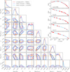 |
Fig. 4 Parameter recovery for an injected mock light curve from the Gaussian AFTERGLOWPY jet model. The corner plot shows the posterior contours at 68 and 95% credibility. Parameters correspond to the symbols in Table 1, σsys is the freely sampled systematic uncertainty. Different colors compare posteriors obtained with different sampling methods. The posterior in red is based on likelihood evaluations from the proper AFTERGLOWPY model with the NMMA sampler. The purple posterior relies on the FIESTA surrogate for the likelihood evaluation but uses the NMMA sampler. The light blue posterior uses the FIESTA surrogate as well but is sampled within FIESTA’s own inference framework that relies on FLOWMC. The injection parameters used to generate the mock light curve data are indicated by the orange lines. The insets on the upper right side show the injection data across the photometric filters and the best-fit light curve (i.e., highest likelihood) of the FIESTA posterior (lightblue) and the actual AFTERGLOWPY light curve used to generate the mock data (red). The latter lies almost completely underneath the former. |
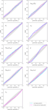 |
Fig. 5 P-P plots for GRB afterglow injections. Each panel shows a P-P plot for the recovery of the parameter displayed in its top left corner. The P-P plots show the cumulative distribution of the injected values’ posterior quantiles for 200 injections. The lightblue curves indicate injection recoveries with AFTERGLOWPY, the magenta ones for PYBLASTAFTER-GLOW. The solid lines signify that the injections stem from physical base model, the dashed lines indicate an injection with the surrogate itself. The gray areas mark the 68-95-99.7% confidence range in which the quantile distribution should fall if it was uniformly distributed. |
4.2 Performance
The computational cost of sampling the posterior, P(θ|d), is mainly determined by the cost of the likelihood function. Using ML surrogates reduces the evaluation time of the likelihood function by several orders of magnitude. This is best illustrated by comparing the total runtime of the inferences shown in Fig. 4, where the posterior for an AFTERGLOWPY injection was obtained with and without the surrogate. The total sampling time with FIESTA amounts to 96 s on an NVIDIA H100 GPU, whereas sampling with the actual AFTERGLOWPY model in NMMA takes 19,700 s (≈5.5 h) on 24 Intel® Xeon® Silver CPUs. Using the power consumption values for the GPUs and CPUs used (NVIDIA Corporation 2023, 2024; Intel Corporation 2022), this implies that inferences with FIESTA consume around 124, respectively, 168 less energy than the equivalent CPU-based run when using the NVIDIA H100, respectively NVIDIA RTX 6000 GPU. This difference is mainly due to the speed-up in the likelihood evaluation and not related to the sampling algorithm, since the run that uses the FIESTA surrogate with the NMMA sampler takes just 203 seconds on the same 24 CPUs. Further, it should be noted that the FLOWMC sampler consists of several stages. First, the likelihood function and the associated neural networks are just-in-time compiled with JAX, which in our inferences takes around 60 s. Then, a training loop takes place which concurrently runs MCMC sampling and training of the normalizing flow proposal, which takes another 30 s. The samples produced during the training loop are considered burn-in samples and are discarded. Generating the final set of posterior samples then only takes about 5 s. The exact length of these different segments depends on the number of datapoints, the hyperparameters of FLOWMC, and the number of photometric filters in the data. The more filters there are, the more often the FLUXMODEL output needs to be converted to AB magnitudes, which involves the evaluation of an integral, thereby decelerating the likelihood evaluation.
Besides the cost of the likelihood function, the size of the parameter space also influences the sampling time. The parameter space at least contains the base model parameters listed in Table 1, but can be extended with parameters to model the systematic uncertainty. As mentioned above, in FIESTA, the systematic uncertainty, σsys, can either be set to a constant value or it can be constructed from a set of sampling parameters. By introducing these nuisance parameters  , the systematic uncertainty can even become time- and filter-dependent through Eq. (5). However, when adding parameters to the sampler, this will impact the sampling time. In Fig. 7, we show how the sampling time (i.e. total runtime minus just-in-time compilation, which remains roughly constant over the cases considered here) per effective sample size of a FIESTA inference evolves when more systematic nuisance parameters are added. While initially the sampling time per effective sample increases notably when going from 10 to 20 sampling dimensions, at a higher dimensionality, the increase remains limited. This is opposite to the behavior of conventional samplers. For instance, in Table II of Jhawar et al. (2025) it is shown that when using the PYMULTI -NEST nested sampler in NMMA, the sampling time increases from 11 minutes when sampling 6 parameters to 107 minutes for a posterior of dimension 21. We of course note that a setting with more than 20 nuisance parameters seems superfluous for real-life data analysis, however, Fig. 7 emphasizes the capability of the FLOWMC sampler to handle large parameter spaces efficiently. This is also useful when combining different models at once, for instance, in joint analyses of GRB afterglow and KN emission.
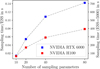 |
Fig. 7 Sampling run time of a FIESTA inference as a function of the parameter space dimension. The plot shows the runtime of a PYBLASTAFTERGLOW injection recovery per effective sample size (ESS) when different numbers of nuisance parameters for the timedependent systematic uncertainty are added. The performance test was conducted on two different GPU types as indicated by the colors in the legend. |
5 Applications
In this section, we apply our newly developed inference framework to two instances of real observations, namely, AT2017gfo/GRB170817A and GRB211112A. We use the bestperforming surrogates from Sect. 3, namely, the FLUXMODEL cVAE’s for the GRB afterglow surrogates and the FLUXMODEL with MLP architecture for the KN surrogate, to jointly analyze the KN emission and GRB afterglow emission in these events.
5.1 AT2017gfo/GRB170817A
As mentioned in Sect. 1, the most prominent instance of a KN and GRB afterglow occurring together is the electromagnetic counterpart to the BNS merger associated with GW170817 (Abbott et al. 2017c,d). We used FIESTA to reanalyze the joint light curve of these events, performing two analyses. One analysis uses our KN surrogate from POSSIS together with the surrogate for the AFTERGLOWPY Gaussian jet, while the other analysis uses the same KN surrogate but together with the PYBLASTAFTERGLOW Gaussian jet surrogate. Our priors are uniform within the ranges specified in Table 1, except for the inclination, where we set ι ~ U(0,π|4) to avoid a second mode at ι ≈ π|2. We confirmed that this second mode is not an artifact from the surrogate, but instead a solution of AFTERGLOWPY to the GRB170817A data, although an inclination of ι > π|4 seems implausible given the observation of the GRB prompt emission and the radio interferometry measurement of the jet inclination angle (Mooley et al. 2018; Ghirlanda et al. 2019; Mooley et al. 2022). The handling of the systematic uncertainty is split between those filters containing the KN observations and those filters containing the GRB afterglow. In particular, we find that the systematic uncertainty around the KN model needs to be represented by four parameters spaced linearly across the KN time interval, each of which is sampled from a uniform prior U(0.5,2). On the other hand, for the GRB afterglow observations only a single systematic uncertainty parameter with a uniform prior U(0.3,2) is needed. The available KN data reach from 0.3 to 24 days, the GRB afterglow data span from 9 to 742 days. We only fit KN data points up to 10 days, since we find that later data points are not well-represented by the POSSIS model. The reason for this behavior is potentially rooted in the breakdown of the local thermodynamical equilibrium in the by-then low-density environment (Waxman et al. 2019; Pognan et al. 2022), which causes the POSSIS predictions to become less applicable. We confirmed that adding the available KN data points at t > 10 days does not significantly alter the posterior. We fixed the luminosity distance at dL = 43.6 Mpc and redshift at z = 0.009727 (Chornock et al. 2017).
In Fig. 8, we show the posterior of our joint KN+GRB afterglow inferences. For the GRB afterglow parameters, we find good agreement between the AFTERGLOWPY and PYBLASTAFTERGLOW models, as well as good agreement compared to previous analyses (Ryan et al. 2020; Pang et al. 2023; Ghirlanda et al. 2019; Troja et al. 2019a). The estimated isotropic kinetic energy from AFTERGLOWPY at  is higher than for PYBLASTAFTERGLOW
  , as is the ambient density with
  from AFTERGLOWPY and
  from PYBLASTAFTER-GLOW. All values are quoted at the 95% level. We attribute this difference to the fact that generally PYBLASTAFTERGLOW light curves are brighter than AFTERGLOWPY light curves due to the different microphysics and radiation scheme. Both analyses find a jet opening angle of about θc = 4−10° and the inclination ι = 23°-44°. This value is partially consistent with analyses that include the displacement of the apparent superluminal centroid to the multiband light curve data (Mooley et al. 2018; Ghirlanda et al. 2019; Mooley et al. 2022), where a range of ι ≈ 14°-28° is inferred. Instead, more recent analyses also find ι = 17.2°-21.2° (Govreen-Segal & Nakar 2023) and ι = 18°-24° (Ryan et al. 2024), which is lower than our estimate. Yet, our credible interval remains consistent with ι ≈ 0°-40° inferred from the GW data alone (Abbott et al. 2017a), using current estimates for the Hubble constant.
The KN parameters offer a more peculiar picture than the afterglow parameters. While the parameters for the ejecta masses broadly agree with estimates from previous works (Anand et al. 2023; Breschi et al. 2024; Pang et al. 2023; Sarin et al. 2024), we find that, in particular, the electron fractions converge to rather extreme values. For both analyses, we find  , and
, and  at 95% credibility. These values contradict the general standard picture in which the dynamical ejecta are neutron-rich, i.e. Ye,dyn ≲ 0.25, and the polar wind ejecta has a higher electron fraction (Metzger & Fernández 2014; Metzger 2020; Shibata & Hotokezaka 2019; Kasen et al. 2017; Nedora et al. 2021). It should be noted, however, that our parameter Y¯e,dyn refers to the mass-averaged electron fraction according to the distribution from Eq. (2) in Anand et al. (2023). Hence, the dynamical ejecta would still contain some portion with low electron fraction. Nevertheless, this value seems high compared to the (uniform) electron fraction in the wind component. The posterior distributions also indicate very low values for υej, wind at the prior edge of 0.05 c, which is in line with previous works (Breschi et al. 2021, 2024; Anand et al. 2023). By comparing the POSSIS training and test data to the AT2017gfo light curve, we confirm that the aforementioned issues are not linked to the performance of our ML surrogate, but instead point towards a systematic issue. Specifically, it seems hard to reconcile the slow descent of the g band with the steep decline of the infrared magnitudes in the 2mass filters. This can be seen in Fig. 9 where we show the best-fit light curves from our analyses for selected filters. Some tension between the bluer and redder components in AT2017gfo has been noted for instance in Breschi et al. (2021) and Hussenot-Desenonges et al. (2025) as well. As mentioned, this might be related to the breakdown of local thermodynamical equilibrium in the late-time ejecta (Waxman et al. 2019; Pognan et al. 2022), or other systematic reasons such as dominance of a few nucleonic decays in the heating process (Kasen & Barnes 2019), unexpected opacity evolution (Kasen & Barnes 2019; Tanaka et al. 2020; Pognan et al. 2022; Gillanders et al. 2024), or ejecta geometry (Collins et al. 2024; King et al. 2025), and emphasizes the need for further research on the early and late KN emission mechanisms.
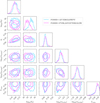 |
Fig. 8 Posterior of the joint KN+GRB afterglow analyses of AT2017gfo/GRB170817A. Selected parameters are shown in the corner plot. The full corner plot can be accessed in our data repository. The lightblue contours indicate the posterior where the GRB afterglow part is fitted with AFTERGLOWPY, magenta is the posterior from PYBLASTAFTERGLOW. Both inferences use the KN surrogate from POSSIS. |
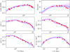 |
Fig. 9 Best-fit light curves from the joint analyses of AT2017gfo/GRB170817A for selected photometric filters. The red data points show their 1σ error bars. The best-fit light curves from the analysis with AFTERGLOWPY (PYBLASTAFTERGLOW) are drawn as solid lines in light-blue (magenta). The colored bands indicate the 1σ systematic uncertainty as determined from the systematic nuisance parameters sampled for this light curve. |
5.2 GRB211211A
GRB211211A was a long GRB observed with the Swift observatory and later associated with a relatively nearby host at ∼ 350 Mpc (Rastinejad et al. 2022). Subsequent analyses of the near-optical and X-ray emission indicated that a KN component was contributing to the emission (Rastinejad et al. 2022; Troja et al. 2022; Mei et al. 2022; Yang et al. 2022; Kunert et al. 2024). We reanalyze the light curve data compiled in Kunert et al. (2024) with FIESTA, using the same surrogates as above for AT2017gfo/GRB170817A. Since the time range of the POSSIS surrogate is restricted to the timespan of 0.226 days and the validity of the POSSIS base model might be restricted to an even smaller time range, we exclude early data points before 0.2 days in the X-ray and uvot filters. We set the priors to be uniform within the ranges from Table 1 and fix the luminosity distance at dL = 358 Mpc and the redshift at z = 0.0763, using Planck18 cosmology (Aghanim et al. 2020). Unlike in AT2017gfo/GRB170817A, the GRB afterglow and KN emission are not featured separately in the light curve data and are superimposed in the UV, optical, and infrared due to the GRB afterglow being seen on axis. Therefore, we sample four systematic nuisance parameters spaced linearly between 0.2-10 days, sampled from a uniform prior U(0.5, 2). For the radio and X-ray band, we set four separate systematic uncertainty parameters that cover the time range from 0.2 to 10 days, sampled from a uniform prior U(0.3,2). This time range is sufficient, even though the X-ray data contain a late data point at 150 days. However, this data point is a detection limit and is fulfilled by our fit regardless of the systematic uncertainty. The posteriors are shown in Fig. 10, the best-fit light curves in Fig. 11. As in the case for GRB170817A, the inferred GRB afterglow parameters do not differ significantly between the analyses with AFTERGLOWPY and PYBLASTAFTERGLOW. The energy from AFTERGLOWPY is again slightly higher as the energy inferred from PYBLASTAFTERGLOW,  compared to
  , which is also the case for the interstellar densities from AFTERGLOWPY
  compared to PYBLASTAFTERGLOW at
  . The microphysical parameters p, εe, and εB are consistent between AFTERGLOWPY and PYBLASTAFTERGLOW.
The KN parameters are relatively unconstrained and some of their marginalized posterior distributions reach down to the lower prior bound. The KN parameters for the dynamical component, i.e., its velocity and electron fraction, essentially recover the prior. The wind ejecta parameters are somewhat better constrained, though still relatively broad with  and
and  . Despite this fact, we find that the KN component is likely needed to explain the data of GRB211211A, as a simple GRB afterglow analysis results in poor fits. Specifically, the reduced chi-squared statistic χ2/ν is 0.24 (0.28) in the joint inference with AFTERGLOWPY (PYBLASTAFTERGLOW) and the KN model, which increases to 1.0 (0.98) when the KN contribution is not included. This is in line with the findings based on Bayesian model selection from Kunert et al. (2024).
In Fig. 10 we also show the results from the analysis of Kunert et al. (2024). Though this analysis also uses the AFTER-GLOWPY Gaussian jet model, unlike our analysis it does not discard early data points before 0.2 days and relies on a different kilonova model (Bulla 2019; Dietrich et al. 2020; Anand et al. 2021; Almualla et al. 2021) with different priors for ejecta masses. Additionally, Kunert et al. (2024) also uses an inclination prior that is dependent on the sampled jet opening angle. Hence, the inferred parameters slightly differ, most notably for the ejecta masses and the interstellar medium density. However, the total ejecta masses mej = mej,dyn − mej,wind obtained from the two different kilonova models are consistent. Our analyses both result in  , while the analysis of Kunert et al. (2024) finds
  . This indicates that even if different assumptions in KN modeling lead to quantitatively different results for the specific model parameters, the total ejecta mass can be inferred consistently.
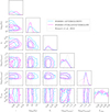 |
Fig. 10 Posterior of the joint KN+GRB afterglow analyses of GRB211211A. Selected parameters are shown in the corner plot. The full corner plot can be accessed in our data repository. The lightblue contours indicate the posterior when the GRB afterglow part is fit with AFTERGLOWPY, magenta is the posterior from PYBLASTAFTERGLOW. Both inferences use the KN surrogate from POSSIS. The lightgrey contours show the analysis from Kunert et al. (2024) as a reference. |
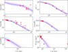 |
Fig. 11 Best-fit light curves from the joint KN+GRB afterglow analyses of GRB211211A for selected photometric filters. Layout as in Fig. 9. Detection limits are shown as triangles. |
6 Discussion and conclusion
The FIESTA package provides ML surrogates of KN and GRB afterglow models to enable efficient likelihood evaluation when sampling a posterior from photometric transient data. It offers a flexible API for training these surrogates, enabling the use of effectively three different architectures. Since FIESTA utilizes the JAX framework, training can be hardware-accelerated by execution on a GPU. Additionally, FIESTA includes functionalities to sample the light curve posterior with FLOWMC (Wong et al. 2023a), an adaptive MCMC sampler that uses gradient-based samplers, and normalizing flow proposals that can also be run on GPUs.
To demonstrate FIESTA’S features, we present surrogates for the AFTERGLOWPY (Ryan et al. 2020) and PYBLASTAFTER-GLOW (Nedora et al. 2025) GRB afterglow models, as well as for the KN model from POSSIS (Bulla 2019, 2023). We find that the surrogates perform well against the respective test data sets, as the prediction error is usually bound within 0.3-0.5 mag. When used during inference, this finite prediction error needs to be offset with a systematic uncertainty, σsys, which can also be sampled in a flexible manner within FIESTA’S implementation. We applied these surrogates to two events with joint KN and GRB afterglow emission, namely AT2017gfo/GRB170817A and GRB211211A. Using our surrogates, we find similar results to previous analyses of these events, even when using the new PYBLASTAFTERGLOW model for the GRB afterglow. However, our posteriors can be evaluated within minutes; whereas previous analyses, for instance, those of Pang et al. (2023); Koehn et al. (2025), could take several hours to days, mainly due to the more expensive likelihood evaluation when computing the light curve directly from AFTERGLOWPY.
Despite the advantages regarding speed when relying on ML surrogates in the likelihood evaluation, this approach also comes with some drawbacks. For one, the parameter ranges in which our surrogates interpolate the training data are fixed and, therefore, it is not possible to extend priors without retraining the surrogates. However, these surrogates can easily be fine-tuned on new training datasets for future use in other places in the parameter space. Further, the prediction error from the surrogate compared to the physical base model could introduce biases in the posteriors. We assessed these potential biases by creating AFTERGLOWPY injection recoveries, where the posterior can be obtained with the surrogate and with the base model. We find that the values for the KL divergence match theoretical expectations within the surrogate uncertainty (Bevins et al. 2025). Furthermore, while we did find biases in the recovery of certain parameters (based on our P-P plots in Figs. 5 and 6), we do not find that this bias is necessarily caused by the use of our surrogates. Still, failure of the surrogate in certain parameter regions cannot be excluded and sanity checks are recommended to validate the results. For instance, the physical base model could be run with the best-fit parameters from the posterior to verify that they actually provide a good fit to the data.
The use of ML techniques for accelerated likelihood evaluation and efficient sampling in Bayesian inference is a common practice in various areas of astrophysics. For instance, the analysis of X-ray spectra has recently been accelerated by the use of advanced stochastic samplers written in JAX (Dupourqué et al. 2024) or with the help of ML surrogate models (Barret & Dupourqué 2024; Tutone et al. 2025; Dupourqué & Barret 2025). For supernovae, Gaussian process surrogate models were developed for inference in Simongini et al. (2024, 2025). Leeney (2025) created a JAX-compatible version of SNCOSMO (Barbary et al. 2025). In FIESTA, we focused on surrogates for electromagnetic transients of BNS mergers; however, in principle, surrogates for other types of transients could also be incorporated. Additionally, as FIESTA surrogates utilize the JAX framework, this opens up the possibility for them to be combined with other JAX software, such as JIM (Wong et al. 2023b; Wouters et al. 2024) for the parameter estimation on GW signals from BNSs. This would enable fast sampling for the joint analysis of GW signals and electromagnetic counterparts and could be linked further to the inference of the EOS for NS matter through the JESTER (Wouters et al. 2025) package, which also leverages JAX to efficiently evaluate the likelihood of an EOS candidate with a given set of NS observations. Additionally, the backward compatibility of our surrogates to NMMA provides the opportunity to perform efficient Bayesian model comparison to either compare transient types (Breschi et al. 2021; Kunert et al. 2024; Hussenot-Desenonges et al. 2024) or to investigate different systematics in the modeling. Such investigations could be related to KN ejecta morphology (Heinzel et al. 2021; King et al. 2025; Hussenot-Desenonges et al. 2025), KN heating rates and opacities (Tanaka et al. 2020; Bulla 2023; Sarin & Rosswog 2024; Brethauer et al. 2024), GRB jet structure (Kunert et al. 2024; Hayes et al. 2020; Lin et al. 2021) or environment (Aksulu et al. 2022), or mappings from BNS parameters to ejecta parameters (Ristic et al. 2025). Given the launch of new transient observatories such as the Vera C. Rubin Observatory (Andreoni et al. 2024) or ULTRASAT (Shvartzvald et al. 2024), the surrogates and accelerated inference techniques presented here could also be used to study different observing strategies to increase the efficiency of parameter estimation (Ragosta et al. 2024; Andrade et al. 2025) and maximize the science output of future detections.
Acknowledgements
We would like to thank the anonymous referee for their helpful suggestions. We would like to thank Kaze Wong for useful discussions and assistance with the FLOWMC package. We would like to thank Nina Kunert for providing the light curve data of GRB211211A. We would like to thank Anna Neuweiler for her assistance with setting up the POSSIS code. Computations were in part performed on the national supercomputer HPE Apollo Hawk at the High Performance Computing Center Stuttgart (HLRS) under the grant number GWanalysis/44189 and on the DFG-funded research cluster jarvis at the University of Potsdam (INST 336/173-1; project number: 502227537). This work used the Dutch national e-infrastructure with the support of the SURF Cooperative using grant no. EINF-8596. H.K., H.R., and T.D. acknowledge funding from the Daimler and Benz Foundation for the project “NUMANJI” and from the European Union (ERC, SMArt, 101076369). T.W. is supported by the research program of the Netherlands Organization for Scientific Research (NWO) under grant number OCENW.XL21.XL21.038. P.T.H.P. is supported by the research program of the Netherlands Organization for Scientific Research (NWO) under grant number VI.Veni.232.021. M.B. acknowledges the Department of Physics and Earth Science of the University of Ferrara for the financial support through the FIRD 2024 grant. Views and opinions expressed are those of the authors only and do not necessarily reflect those of the European Union or the European Research Council. Neither the European Union nor the granting authority can be held responsible for them.
References
- Abbott, B. P., Abbott, R., Abbott, T. D., et al. 2017a, Nature, 551, 85 [Google Scholar]
- Abbott, B. P., Abbott, R., Abbott, T., et al. 2017b, ApJ, 848, L13 [CrossRef] [Google Scholar]
- Abbott, B. P., Abbott, R., Abbott, T., et al. 2017c, PRL, 119, 161101 [Google Scholar]
- Abbott, B. P., Abbott, R., Abbott, T., et al. 2017d, ApJ, 848, L12 [Google Scholar]
- Aghanim, N., Akrami, Y., Ashdown, M., et al. 2020, A&A, 641, A6 [Erratum: A&A 652, C4 (2021)] [NASA ADS] [CrossRef] [EDP Sciences] [Google Scholar]
- Ahumada, T., Anand, S., Bulla, M., et al. 2025, arXiv e-prints [arXiv:2507.00357] [Google Scholar]
- Aksulu, M. D., Wijers, R. A. M. J., van Eerten, H. J., & van der Horst, A. J. 2020, MNRAS, 497, 4672 [NASA ADS] [CrossRef] [Google Scholar]
- Aksulu, M. D., Wijers, R. A. M. J., van Eerten, H. J., & van der Horst, A. J. 2022, MNRAS, 511, 2848 [NASA ADS] [CrossRef] [Google Scholar]
- Almualla, M., Ning, Y., Salehi, P., et al. 2021, arXiv e-prints [arXiv:2112.15470] [Google Scholar]
- Anand, S., Coughlin, M. W., Kasliwal, M. M., et al. 2021, Nat. Astron., 5, 46 [NASA ADS] [CrossRef] [Google Scholar]
- Anand, S., Coughlin, M. W., Kasliwal, M. M., et al. 2023, arXiv e-prints [arXiv:2307.11080] [Google Scholar]
- Andrade, C., Alserkal, R., Manzano, L. S., et al. 2025, Publ. Astron. Soc. Pac., 137, 034102 [Google Scholar]
- Andreoni, I., Ackley, K., Cooke, J., et al. 2017, Publ. Astron. Soc. Austral., 34, e069 [Google Scholar]
- Andreoni, I., Ackley, K., Cooke, J., et al. 2024 arXiv e-prints [arXiv:2411.04793] [Google Scholar]
- Annala, E., Gorda, T., Katerini, E., et al. 2022, PRX, 12, 011058 [Google Scholar]
- Ascenzi, S., Coughlin, M. W., Dietrich, T., et al. 2019, MNRAS, 486, 672 [Google Scholar]
- Barbary, K., Bailey, S., Barentsen, G., et al. 2025, SNCosmo [Google Scholar]
- Barret, D., & Dupourqué, S. 2024, A&A, 686, A133 [NASA ADS] [CrossRef] [EDP Sciences] [Google Scholar]
- Bevins, H. T. J., Gessey-Jones, T., & Handley, W. J. 2025, MNRAS, 544, 375 [Google Scholar]
- Boersma, O. M., & van Leeuwen, J. 2023, Pub. Astron. Soc. Austr., 40, e30 [Google Scholar]
- Breschi, M., Perego, A., Bernuzzi, S., et al. 2021, MNRAS, 505, 1661 [NASA ADS] [CrossRef] [Google Scholar]
- Breschi, M., Gamba, R., Carullo, G., et al. 2024, A&A, 689, A51 [NASA ADS] [CrossRef] [EDP Sciences] [Google Scholar]
- Brethauer, D., Kasen, D., Margutti, R., & Chornock, R. 2024, ApJ, 975, 213 [NASA ADS] [CrossRef] [Google Scholar]
- Bulla, M. 2019, MNRAS, 489, 5037 [NASA ADS] [CrossRef] [Google Scholar]
- Bulla, M. 2023, MNRAS, 520, 2558 [CrossRef] [Google Scholar]
- Chornock, R., Berger, E., Kasen, D., et al. 2017, ApJ, 848, L19 [NASA ADS] [CrossRef] [Google Scholar]
- Collins, C. E., Shingles, L. J., Bauswein, A., et al. 2024, MNRAS, 529, 1333 [NASA ADS] [CrossRef] [Google Scholar]
- Coulter, D. A., Foley, R. J., Kilpatrick, C. D., et al. 2017, Science, 358, 1556 [NASA ADS] [CrossRef] [Google Scholar]
- Curtis, S., Mösta, P., Wu, Z., et al. 2022, MNRAS, 518, 5313 [Google Scholar]
- Dax, M., Green, S. R., Gair, J., et al. 2025, Nature, 639, 49 [Google Scholar]
- Díaz, M. C., Macri, L. M., Lambas, D. G., et al. 2017, ApJ, 848, L29 [Google Scholar]
- Dietrich, T., Coughlin, M. W., Pang, P. T. H., et al. 2020, Science, 370, 1450 [Google Scholar]
- Dupourqué, S., & Barret, D. 2025, A&A, 699, A179 [NASA ADS] [CrossRef] [EDP Sciences] [Google Scholar]
- Dupourqué, S., Barret, D., Diez, C. M., Guillot, S., & Quintin, E. 2024, A&A, 690, A317 [NASA ADS] [CrossRef] [EDP Sciences] [Google Scholar]
- Feroz, F., Hobson, M. P., & Bridges, M. 2009, MNRAS, 398, 1601 [NASA ADS] [CrossRef] [Google Scholar]
- Ford, N. M., Vieira, N., Ruan, J. J., & Haggard, D. 2024, ApJ, 961, 119 [Google Scholar]
- Gabrié, M., Rotskoff, G. M., & Vanden-Eijnden, E. 2022, PNAS, 119, e2109420119 [Google Scholar]
- Ghirlanda, G., Salafia, O. S., Paragi, Z., et al. 2019, Science, 363, 968 [NASA ADS] [CrossRef] [Google Scholar]
- Gianfagna, G., Piro, L., Pannarale, F., et al. 2024, MNRAS, 528, 2600 [Google Scholar]
- Gillanders, J. H., Sim, S. A., Smartt, S. J., Goriely, S., & Bauswein, A. 2024, MNRAS, 529, 2918 [NASA ADS] [CrossRef] [Google Scholar]
- Goldstein, A., et al. 2017, ApJ, 848, L14 [CrossRef] [Google Scholar]
- Govreen-Segal, T., & Nakar, E. 2023, MNRAS, 524, 403 [NASA ADS] [CrossRef] [Google Scholar]
- Grenander, U., & Miller, M. I. 1994, J. R. Stat. Soc. Ser. B , 56, 549 [Google Scholar]
- Guillochon, J., Nicholl, M., Villar, V. A., et al. 2018, ApJS, 236, 6 [NASA ADS] [CrossRef] [Google Scholar]
- Güven, H., Bozkurt, K., Khan, E., & Margueron, J. 2020, PRC, 102, 015805 [Google Scholar]
- Hayes, F., Heng, I. S., Veitch, J., & Williams, D. 2020, ApJ, 891, 124 [NASA ADS] [CrossRef] [Google Scholar]
- Heek, J., Levskaya, A., Oliver, A., et al. 2024, Flax: A neural network library and ecosystem for JAX [Google Scholar]
- Heinzel, J., Coughlin, M. W., Dietrich, T., et al. 2021, MNRAS, 502, 3057 [CrossRef] [Google Scholar]
- Hotokezaka, K., Nakar, E., Gottlieb, O., et al. 2019, Nat. Astron., 3, 940 [NASA ADS] [CrossRef] [Google Scholar]
- Hu, Q., Irwin, J., Sun, Q., et al. 2025, ApJ, 987, L17 [Google Scholar]
- Humphrey, P. J., Liu, W., & Buote, D. A. 2009, ApJ, 693, 822 [Google Scholar]
- Hussenot-Desenonges, T., Wouters, T., Guessoum, N., et al. 2024, MNRAS, 530, 1 [NASA ADS] [CrossRef] [Google Scholar]
- Hussenot-Desenonges, T., Pillas, M., Antier, S., Hello, P., & Pang, P. T. H. 2025, arXiv e-prints [arXiv:2505.21392] [Google Scholar]
- Intel Corporation 2022, Intel® Xeon® Silver 4310 Processor: 18M Cache, 2.10 GHz, accessed: 2025-07-17 [Google Scholar]
- Jhawar, S., Wouters, T., Pang, P. T. H., et al. 2025, PRD, 111, 043046 [Google Scholar]
- Kasen, D., & Barnes, J. 2019, ApJ, 876, 128 [Google Scholar]
- Kasen, D., Metzger, B., Barnes, J., Quataert, E., & Ramirez-Ruiz, E. 2017, Nature, 551, 80 [Google Scholar]
- Kawaguchi, K., Shibata, M., & Tanaka, M. 2018, ApJ, 865, L21 [NASA ADS] [CrossRef] [Google Scholar]
- Kawaguchi, K., Shibata, M., & Tanaka, M. 2020, ApJ, 889, 171 [NASA ADS] [CrossRef] [Google Scholar]
- Kedia, A., Ristic, M., O’Shaughnessy, R., et al. 2023, Phys. Rev. Res., 5, 013168 [Google Scholar]
- King, B. L., De, S., Korobkin, O., Coughlin, M. W., & Pang, P. T. H. 2025, PASP, 137, 104507 [Google Scholar]
- Kingma, D. P., & Welling, M. 2013, arXiv e-prints [arXiv:1312.6114] [Google Scholar]
- Kiuchi, K., Kawaguchi, K., Kyutoku, K., et al. 2017, PRD, 96, 084060 [Google Scholar]
- Kobyzev, I., Prince, S. J., & Brubaker, M. A. 2020, IEEE Trans. Pattern Anal. Mach. Intell., 43, 3964 [Google Scholar]
- Koehn, H., Rose, H., Pang, P. T. H., et al. 2025, PRX, 15, 021014 [Google Scholar]
- Kunert, N., Antier, S., Nedora, V., et al. 2024, MNRAS, 527, 3900 [Google Scholar]
- Lamb, G. P., Mandel, I., & Resmi, L. 2018, MNRAS, 481, 2581 [CrossRef] [Google Scholar]
- Leeney, S. A. K. 2025, arXiv e-prints [arXiv:2504.08081] [Google Scholar]
- Levan, A. J., Malesani, D. B., Gompertz, B. P., et al. 2023, Nat. Astron., 7, 976 [NASA ADS] [CrossRef] [Google Scholar]
- Levan, A. J., Gompertz, B. P., Salafia, O. S., et al. 2024, Nature, 626, 737 [NASA ADS] [CrossRef] [Google Scholar]
- Lin, E.-T., Hayes, F., Lamb, G. P., et al. 2021, Universe, 7, 349 [Google Scholar]
- Lipunov, V. M., Gorbovskoy, E., Kornilov, V. G., et al. 2017, ApJ, 850, L1 [NASA ADS] [CrossRef] [Google Scholar]
- Lukosiüte, K., Raaijmakers, G., Doctor, Z., Soares-Santos, M., & Nord, B. 2022, MNRAS, 516, 1137 [Google Scholar]
- Marinari, E., & Parisi, G. 1992, EPL, 19, 451 [Google Scholar]
- McEwen, J. D., Wallis, C. G. R., Price, M. A., & Mancini, A. S. 2023, arXiv e-prints [arXiv:2111.12720] [Google Scholar]
- Mei, A., Banerjee, B., Oganesyan, G., et al. 2022, Nature, 612, 236 [NASA ADS] [CrossRef] [Google Scholar]
- Metzger, B. D. 2020, Liv. Rev. Rel., 23, 1 [Google Scholar]
- Metzger, B. D., & Fernández, R. 2014, MNRAS, 441, 3444 [CrossRef] [Google Scholar]
- Miceli, D., & Nava, L. 2022, Galaxies, 10, 66 [NASA ADS] [CrossRef] [Google Scholar]
- Mooley, K. P., Deller, A. T., Gottlieb, O., et al. 2018, Nature, 561, 355 [Google Scholar]
- Mooley, K. P., Anderson, J., & Lu, W. 2022, Nature, 610, 273 [NASA ADS] [CrossRef] [Google Scholar]
- Mukherjee, S., Lavaux, G., Bouchet, F. R., et al. 2021, A&A, 646, A65 [NASA ADS] [CrossRef] [EDP Sciences] [Google Scholar]
- Nava, L., Sironi, L., Ghisellini, G., Celotti, A., & Ghirlanda, G. 2013, MNRAS, 433, 2107 [NASA ADS] [CrossRef] [Google Scholar]
- Neal, R. M. 2011, Handbook of Markov Chain Monte Carlo (Boca Raton: CRC Press) [Google Scholar]
- Nedora, V., Bernuzzi, S., Radice, D., et al. 2021, ApJ, 906, 98 [NASA ADS] [CrossRef] [Google Scholar]
- Nedora, V., Menegazzi, L. C., Peretti, E., Dietrich, T., & Shibata, M. 2025, MNRAS, 538, 2089 [Google Scholar]
- Newton, M., & Raftery, A. 1994, J. R. Stat. Soc. Ser. B, 56, 3 [Google Scholar]
- Nicholl, M., Margalit, B., Schmidt, P., et al. 2021, MNRAS, 505, 3016 [NASA ADS] [CrossRef] [Google Scholar]
- NVIDIA Corporation 2023, NVIDIA RTX 6000 Ada Generation Datasheet, accessed: 2025-07-17 [Google Scholar]
- NVIDIA Corporation 2024, NVIDIA H100 Tensor Core GPU, accessed: 202507-17 [Google Scholar]
- Pang, P. T. H., Dietrich, T., Coughlin, M. W., et al. 2023, Nat. Commun., 14, 8352 [Google Scholar]
- Papamakarios, G., Nalisnick, E., Rezende, D. J., Mohamed, S., & Lakshminarayanan, B. 2021, J. Mach. Learn. Res., 22, 2617 [Google Scholar]
- Pellouin, C., & Daigne, F. 2024, A&A, 690, A281 [NASA ADS] [CrossRef] [EDP Sciences] [Google Scholar]
- Peng, Y., Ristic, M., Kedia, A., et al. 2024, Phys. Rev. Res., 6, 033078 [Google Scholar]
- Pognan, Q., Jerkstrand, A., & Grumer, J. 2022, MNRAS, 513, 5174 [NASA ADS] [CrossRef] [Google Scholar]
- Polanska, A., Price, M. A., Piras, D., Spurio Mancini, A., & McEwen, J. D. 2025, OJAp, 8 [Google Scholar]
- Raaijmakers, G., Greif, S. K., Hebeler, K., et al. 2021, ApJ, 918, L29 [NASA ADS] [CrossRef] [Google Scholar]
- Radice, D., Perego, A., Hotokezaka, K., et al. 2018a, ApJ, 869, 130 [Google Scholar]
- Radice, D., Perego, A., Zappa, F., & Bernuzzi, S. 2018b, ApJ, 852, L29 [NASA ADS] [CrossRef] [Google Scholar]
- Ragosta, F., Ahumada, T., Piranomonte, S., et al. 2024, ApJ, 966, 214 [Google Scholar]
- Rastinejad, J. C., et al. 2022, Nature, 612, 223 [NASA ADS] [CrossRef] [Google Scholar]
- Rezende, D. J., & Mohamed, S. 2015, arXiv e-prints [arXiv:1505.05770] [Google Scholar]
- Rezende, D. J., Mohamed, S., & Wierstra, D. 2014, in Proceedings of the 31st International Conference on Machine Learning (ICML) [Google Scholar]
- Rinaldi, E., Fraija, N., & Dainotti, M. G. 2024, Galaxies, 12, 5 [Google Scholar]
- Ristic, M., Champion, E., O’Shaughnessy, R., et al. 2022, Phys. Rev. Res., 4, 013046 [Google Scholar]
- Ristic, M., O’Shaughnessy, R., Villar, V. A., et al. 2023, Phys. Rev. Res., 5, 043106 [Google Scholar]
- Ristic, M., O’Shaughnessy, R., Wagner, K., et al. 2025, arXiv e-prints [arXiv:2503.12320] [Google Scholar]
- Ryan, G., van Eerten, H., MacFadyen, A., & Zhang, B.-B. 2015, ApJ, 799, 3 [NASA ADS] [CrossRef] [Google Scholar]
- Ryan, G., van Eerten, H., Piro, L., & Troja, E. 2020, ApJ, 896, 166 [CrossRef] [Google Scholar]
- Ryan, G., van Eerten, H., Troja, E., et al. 2024, ApJ, 975, 131 [Google Scholar]
- Saha, S., et al. 2024, ApJ, 961, 165 [Google Scholar]
- Salafia, O. S., & Ghirlanda, G. 2022, Galaxies, 10, 93 [NASA ADS] [CrossRef] [Google Scholar]
- Sarin, N., & Rosswog, S. 2024, ApJ, 973, L24 [Google Scholar]
- Sarin, N., Ashton, G., Lasky, P. D., et al. 2021, arXiv e-prints [arXiv:2105.10108] [Google Scholar]
- Sarin, N., Hübner, M., Omand, C. M. B., et al. 2024, MNRAS, 531, 1203 [NASA ADS] [CrossRef] [Google Scholar]
- Savchenko, V., Ferrigno, C., Kuulkers, E., et al. 2017, ApJ, 848, L15 [NASA ADS] [CrossRef] [Google Scholar]
- Setzer, C. N., Peiris, H. V., Korobkin, O., & Rosswog, S. 2023, MNRAS, 520, 2829 [Google Scholar]
- Shappee, B. J., Simon, J. D., Drout, M. R., et al. 2017, Science, 358, 1574 [NASA ADS] [CrossRef] [Google Scholar]
- Shibata, M., & Hotokezaka, K. 2019, Ann. Rev. Nucl. Part. Sci., 69, 41 [NASA ADS] [CrossRef] [Google Scholar]
- Shvartzvald, Y., Waxman, E., Gal-Yam, A., et al. 2024, ApJ, 964, 74 [NASA ADS] [CrossRef] [Google Scholar]
- Simongini, A., Ragosta, F., Piranomonte, S., & Di Palma, I. 2024, MNRAS, 533, 3053 [Google Scholar]
- Simongini, A., Ragosta, F., Piranomonte, S., & Di Palma, I. 2025, EPJ Web Conf., 319, 13002 [Google Scholar]
- Skilling, J. 2004, AIP Conf. Proc., 735, 395 [Google Scholar]
- Skilling, J. 2006, Bayesian Anal., 1, 833 [Google Scholar]
- Soares-Santos, M., Holz, D. E., Annis, J., et al. 2017, ApJ, 848, L16 [CrossRef] [Google Scholar]
- Speagle, J. S. 2020, MNRAS, 493, 3132 [Google Scholar]
- Stratta, G., Nicuesa Guelbenzu, A. M., Klose, S., et al. 2025, ApJ, 979, 159 [Google Scholar]
- Tanaka, M., Kato, D., Gaigalas, G., & Kawaguchi, K. 2020, MNRAS, 496, 1369 [NASA ADS] [CrossRef] [Google Scholar]
- Tanvir, N. R., Levan, A. J., Fruchter, A. S., et al. 2013, Nature, 500, 547 [CrossRef] [Google Scholar]
- Tanvir, N. R., Levan, A. J., González-Fernández, C., et al. 2017, ApJ, 848, L27 [CrossRef] [Google Scholar]
- Thielemann, F. K., Arcones, A., Käppeli, R., et al. 2011, Prog. Part. Nucl. Phys., 66, 346 [NASA ADS] [CrossRef] [Google Scholar]
- Troja, E., Ryan, G., Piro, L., et al. 2018, Nat. Commun., 9, 4089 [NASA ADS] [CrossRef] [Google Scholar]
- Troja, E., van Eerten, H., Ryan, G., et al. 2019a, MNRAS, 489, 1919 [NASA ADS] [Google Scholar]
- Troja, E., Castro-Tirado, A. J., González, J. B., et al. 2019b, MNRAS, 489, 2104 [Erratum: MNRAS 490, 4367 (2019)] [NASA ADS] [Google Scholar]
- Troja, E., Fryer, C.L., O’Connor, B., et al. 2022, Nature, 612, 228 [NASA ADS] [CrossRef] [Google Scholar]
- Tutone, A., Anitra, A., Ambrosi, E., et al. 2025, A&A, 696, A77 [NASA ADS] [CrossRef] [EDP Sciences] [Google Scholar]
- Utsumi, Y., Tanaka, M., Tominaga, N., et al. 2017, Publ. Astron. Soc. Jap., 69, 101 [Google Scholar]
- Valenti, S., Sand, D. J., Yang, S., et al. 2017, ApJ, 848, L24 [CrossRef] [Google Scholar]
- van Eerten, H. J., van der Horst, A. J., & MacFadyen, A. I. 2012, ApJ, 749, 44 [NASA ADS] [CrossRef] [Google Scholar]
- Villar, V. A., Guillochon, J., Berger, E. et al. 2017, ApJ, 851, L21 [CrossRef] [Google Scholar]
- Wallace, W. F., & Sarin, N. 2025, MNRAS, 539, 3319 [Google Scholar]
- Wang, H., & Giannios, D. 2021, ApJ, 908, 200 [Google Scholar]
- Wang, H., Dastidar, R. G., Giannios, D., & Duffell, P. C. 2024, ApJS, 273, 17 [Google Scholar]
- Wang, Y., Chen, C., & Zhang, B. 2026, JHEAp, 50, 100490 [Google Scholar]
- Warren, D. C., Dainotti, M., Barkov, M. V., et al. 2022, ApJ, 924, 40 [NASA ADS] [CrossRef] [Google Scholar]
- Waxman, E., Ofek, E. O., & Kushnir, D. 2019, ApJ, 878, 93 [Google Scholar]
- Wollaeger, R. T., Fryer, C. L., Chase, E. A., et al. 2021, ApJ, 918, 10 [Google Scholar]
- Wong, K. W. k., Gabrié, M., & Foreman-Mackey, D. 2023a, JOSS, 8, 5021 [Google Scholar]
- Wong, K. W. K., Isi, M., & Edwards, T. D. P. 2023b, ApJ, 958, 129 [NASA ADS] [CrossRef] [Google Scholar]
- Wouters, T., Pang, P. T. H., Dietrich, T., & Van Den Broeck, C. 2024, PRD, 110, 083033 [Google Scholar]
- Wouters, T., Pang, P. T. H., Koehn, H., et al. 2025, PRD, 112, 043037 [Google Scholar]
- Wysocki, D., O’Shaughnessy, R., Lange, J., & Fang, Y.-L. L. 2019, PRD, 99, 084026 [Google Scholar]
- Yang, J., Ai, S., Zhang, B.-B., et al. 2022, Nature, 612, 232 [NASA ADS] [CrossRef] [Google Scholar]
- Yang, Y.-H., Troja, E., O’Connor, B., et al. 2024, Nature, 626, 742 [NASA ADS] [CrossRef] [Google Scholar]
- Zhang, B. T., Murase, K., Yuan, C., Kimura, S. S., & Mészáros, P. 2021, ApJ, 908, L36 [NASA ADS] [CrossRef] [Google Scholar]
Appendix A GRB afterglow tophat jet surrogates
In this appendix, we present the benchmarks of the surrogates for the tophat jet models of AFTERGLOWPY and PYBLASTAFTER-GLOW. Figures A.1 and A.2 show the distribution of the prediction error of the surrogate against a test data set. The different architectures are shown again as different colors. In general, all trained surrogates perform well, as the typical mean squared error across the entire light curve is < 0.1 mag across all filters. The only exception is the X-ray filter for PYBLASTAFTERGLOW, but this can be attributed again to the hard cut below 2 · 10−22 mJy we imposed on the training data (see Sect. 3.2).
For AFTERGLOWPY, the MLP surrogate performs noticeably worse than the surrogate with a cVAE architecture, especially at later times. Considering some example light curves, we find that the reason for this is likely due to the fact that the MLP architecture performs worse when a counterjet causes a late bump in the light curve, whereas the cVAE does not struggle with this feature as much. However, the counterjet contribution is also incorporated in the Gaussian models above and in the PYBLASTAFTER-GLOW tophat model, where the MLP and cVAE perform similarly. For both AFTERGLOWPY and PYBLASTAFTERGLOW, the absolute mismatch across the light curve of the cVAE surrogate is typically confined within 0.2 mag, except again in the X-ray filter for PYBLASTAFTERGLOW. For the AFTERGLOWPY cVAE, 95% of test predictions are always within 1 mag of the proper light curve; for the PYBLASTAFTERGLOW cVAE it is even 97%.
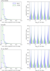 |
Fig. A.1 Benchmarks of the two surrogates for the AFTERGLOWPY tophat jet model. We show the deviations of surrogate predictions against a test data set of size ntest = 7500. Figure layout is the same as in Fig. 1. |
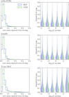 |
Fig. A.2 Benchmarks of the two surrogates for the PYBLASTAFTERGLOW tophat jet model. We show the deviations of surrogate predictions against a test data set of size ntest = 7680. Figure layout is the same as in Fig. 1. |
Appendix B Injection recoveries for the PYBLASTAFTERGLOW and POSSIS surrogates
In Fig. B.1, we show the posterior corner plots from an injection with the PYBLASTAFTERGLOW afterglow model. Likewise, in Fig. B.2 we show the posterior from an injection with POSSIS. The meaning of the respective parameters is given in Table 1, the priors are uniform within the ranges specified there. We set the prior for σsys to be uniform from 0.3 to 1 mag in case of the PYBLASTAFTERGLOW inference and uniform from 0.5 to 1 mag in case of the POSSIS inference, since for the latter the surrogate is expected to have slightly larger prediction errors. We find that the true injected values are well recovered in both cases. For the recovery of the PYBLASTAFTERGLOW injection, we find that σsys, sampled from a uniform prior U(0.3,1) converges to a value slightly larger than the lower prior bound. We attribute this to the late bump in the PYBLASTAFTERGLOW light curve at 100150 days that is not accurately accounted for by the surrogate in the optical. On this interval, the surrogate deviates from the true light curve by about 0.4 mag, which the systematic uncertainty takes into account. However, this only works because the surrogate matches the other parts of the light curve within 0.3 mag and the larger deviation is confined to a small segment. In general, sampling σsys without a sufficiently high prior bound may fail to adequately capture the surrogate prediction error.
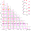 |
Fig. B.1 Parameter recovery for an injected mock light curve from the Gaussian PYBLASTAFTERGLOW jet model. Figure layout as in Fig. 4. The injection is from the PYBLASTAFTERGLOW base model, the recovery is with the FIESTA surrogate and the FLOWMC sampler. |
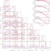 |
Fig. B.2 Parameter recovery for an injected mock light curve from the Gaussian pyblastafterglow jet model. Figure layout as in Fig. 4. The injection is from the POSSIS directly, the recovery is with the fiesta surrogate and the flowMC sampler. The insets on the upper right side show the injection data with the best-fit light curve (purple) and the true POSSIS light curve (red). Triangles indicate upper mock detection limits at 24 mag placed to prevent the surrogate being used on parts of the light curve where the training data is subject to Monte Carlo noise. |
All Tables
All Figures
|
Fig. 1 Benchmarks of the two surrogates for the AFTERGLOWPY Gaussian jet model. We show the error distributions of the surrogate predictions against a test data set of size ntest = 7500. The different rows show the error across different passbands. The left panels show the distribution of the mean squared error as defined in Eq. (9). The right panels show the mismatch distribution across the test data set as defined in Eq. (10). The figure compares two different surrogates: one using the MLP architecture (blue) and the other a cVAE (green). |
| In the text | |
|
Fig. 2 Benchmarks of the two surrogates for the PYBLASTAFTERGLOW Gaussian jet model. We show the deviations of surrogate predictions against a test data set of size ntest = 7232. Figure layout is the same as in Fig. 1. |
| In the text | |
|
Fig. 3 Benchmarks of two surrogates for the KN POSSIS model. We show the deviations of surrogate predictions against a test data set of size ntest = 2238. Figure layout as in Fig. 1. The figure compares two different surrogates: one using the MLP architecture (blue) and the other a LIGHTCURVEMODEL, where an MLP is trained for each passband separately (green). |
| In the text | |
|
Fig. 4 Parameter recovery for an injected mock light curve from the Gaussian AFTERGLOWPY jet model. The corner plot shows the posterior contours at 68 and 95% credibility. Parameters correspond to the symbols in Table 1, σsys is the freely sampled systematic uncertainty. Different colors compare posteriors obtained with different sampling methods. The posterior in red is based on likelihood evaluations from the proper AFTERGLOWPY model with the NMMA sampler. The purple posterior relies on the FIESTA surrogate for the likelihood evaluation but uses the NMMA sampler. The light blue posterior uses the FIESTA surrogate as well but is sampled within FIESTA’s own inference framework that relies on FLOWMC. The injection parameters used to generate the mock light curve data are indicated by the orange lines. The insets on the upper right side show the injection data across the photometric filters and the best-fit light curve (i.e., highest likelihood) of the FIESTA posterior (lightblue) and the actual AFTERGLOWPY light curve used to generate the mock data (red). The latter lies almost completely underneath the former. |
| In the text | |
|
Fig. 5 P-P plots for GRB afterglow injections. Each panel shows a P-P plot for the recovery of the parameter displayed in its top left corner. The P-P plots show the cumulative distribution of the injected values’ posterior quantiles for 200 injections. The lightblue curves indicate injection recoveries with AFTERGLOWPY, the magenta ones for PYBLASTAFTER-GLOW. The solid lines signify that the injections stem from physical base model, the dashed lines indicate an injection with the surrogate itself. The gray areas mark the 68-95-99.7% confidence range in which the quantile distribution should fall if it was uniformly distributed. |
| In the text | |
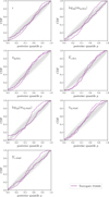 |
Fig. 6 P-P plots for the POSSIS surrogate model. Figure layout as in Fig. 5. |
| In the text | |
|
Fig. 7 Sampling run time of a FIESTA inference as a function of the parameter space dimension. The plot shows the runtime of a PYBLASTAFTERGLOW injection recovery per effective sample size (ESS) when different numbers of nuisance parameters for the timedependent systematic uncertainty are added. The performance test was conducted on two different GPU types as indicated by the colors in the legend. |
| In the text | |
|
Fig. 8 Posterior of the joint KN+GRB afterglow analyses of AT2017gfo/GRB170817A. Selected parameters are shown in the corner plot. The full corner plot can be accessed in our data repository. The lightblue contours indicate the posterior where the GRB afterglow part is fitted with AFTERGLOWPY, magenta is the posterior from PYBLASTAFTERGLOW. Both inferences use the KN surrogate from POSSIS. |
| In the text | |
|
Fig. 9 Best-fit light curves from the joint analyses of AT2017gfo/GRB170817A for selected photometric filters. The red data points show their 1σ error bars. The best-fit light curves from the analysis with AFTERGLOWPY (PYBLASTAFTERGLOW) are drawn as solid lines in light-blue (magenta). The colored bands indicate the 1σ systematic uncertainty as determined from the systematic nuisance parameters sampled for this light curve. |
| In the text | |
|
Fig. 10 Posterior of the joint KN+GRB afterglow analyses of GRB211211A. Selected parameters are shown in the corner plot. The full corner plot can be accessed in our data repository. The lightblue contours indicate the posterior when the GRB afterglow part is fit with AFTERGLOWPY, magenta is the posterior from PYBLASTAFTERGLOW. Both inferences use the KN surrogate from POSSIS. The lightgrey contours show the analysis from Kunert et al. (2024) as a reference. |
| In the text | |
|
Fig. 11 Best-fit light curves from the joint KN+GRB afterglow analyses of GRB211211A for selected photometric filters. Layout as in Fig. 9. Detection limits are shown as triangles. |
| In the text | |
|
Fig. A.1 Benchmarks of the two surrogates for the AFTERGLOWPY tophat jet model. We show the deviations of surrogate predictions against a test data set of size ntest = 7500. Figure layout is the same as in Fig. 1. |
| In the text | |
|
Fig. A.2 Benchmarks of the two surrogates for the PYBLASTAFTERGLOW tophat jet model. We show the deviations of surrogate predictions against a test data set of size ntest = 7680. Figure layout is the same as in Fig. 1. |
| In the text | |
|
Fig. B.1 Parameter recovery for an injected mock light curve from the Gaussian PYBLASTAFTERGLOW jet model. Figure layout as in Fig. 4. The injection is from the PYBLASTAFTERGLOW base model, the recovery is with the FIESTA surrogate and the FLOWMC sampler. |
| In the text | |
|
Fig. B.2 Parameter recovery for an injected mock light curve from the Gaussian pyblastafterglow jet model. Figure layout as in Fig. 4. The injection is from the POSSIS directly, the recovery is with the fiesta surrogate and the flowMC sampler. The insets on the upper right side show the injection data with the best-fit light curve (purple) and the true POSSIS light curve (red). Triangles indicate upper mock detection limits at 24 mag placed to prevent the surrogate being used on parts of the light curve where the training data is subject to Monte Carlo noise. |
| In the text | |
Current usage metrics show cumulative count of Article Views (full-text article views including HTML views, PDF and ePub downloads, according to the available data) and Abstracts Views on Vision4Press platform.
Data correspond to usage on the plateform after 2015. The current usage metrics is available 48-96 hours after online publication and is updated daily on week days.
Initial download of the metrics may take a while.