© The Authors 2025

1. Introduction

It is now widely accepted within the cosmological community that there existed an epoch of rapid space-time expansion in the early Universe, which is referred to as inflation. This inflationary epoch is characterized by exponential growth of the scale factor in such a way that neatly explains the isotropy and homogeneity we observe in the large-scale structure (LSS) today. The driving mechanism for inflation is believed to be scalar field oscillations (Guth 1981; Linde 1982; Albrecht & Steinhardt 1982). Despite the remarkable theoretical success of inflation in its ability to solve the horizon and flatness problems (Guth 1981), among others, its detailed characteristics are not well constrained. Thus, we turn to observational probes.

In the simplest inflationary scenario, involving a single scalar field, overdensities in the cosmic-matter-density profile are expected to follow a Gaussian distribution (Maldacena 2003). Conversely, multi-field models predict varying degrees of deviation from Gaussianity (Creminelli et al. 2011). To distinguish between these models and refine our understanding of the early Universe, we relied on measurements of local primordial non-Gaussianity (PNG).

The primordial gravitational potential for a general scalar field model can be expressed as

$$\begin{array}{c}\hfill {\mathrm{\Phi }}_{\text{NG}}=\varphi +f_{\text{NL}}({\varphi }^2-{⟨\varphi ⟩}^2),\end{array}$$(1)

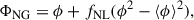
where ϕ represents the potential of a Gaussian random field, and f_NL (this is really $f_{\text{NL}}^{\text{loc}}$, the local PNG parameter, but we refer to it simply as f_NL throughout) quantifies the amplitude of the quadratic deviation in the potential (Komatsu & Spergel 2001; Gangui et al. 1994). A nonzero value of f_NL indicates deviations from the single-field model. Consequently, constraining f_NL is a key step in testing inflationary models.

Significant efforts have been made to measure f_NL. One of the primary methods involves analyzing anisotropies in the cosmic microwave background (CMB), with the Planck bispectrum analysis providing the tightest constraint to date: f_NL = 0.9 ± 5.1 (68% confidence limits) (Planck Collaboration IX 2020). While this has ruled out some highly non-Gaussian multi-field models, achieving greater precision is necessary to further narrow down the model parameter space. Moreover, CMB-based analyses are fundamentally limited by cosmic variance (e.g., Kalaja et al. 2021).

Alternative approaches to probing PNG involve the LSS, offering opportunities for cross-validation and potentially greater sensitivity to f_NL. These methods analyze the distribution of galaxy clusters and dark-matter (DM) halos through the power spectrum and bispectrum, among higher order statistics (see, e.g., Ross et al. 2013; Castorina et al. 2019; Mueller et al. 2022; Cagliari et al. 2025), which are Fourier transforms of the configuration-space two-point, three-point, and higher order correlation functions (2pcf, 3pcf, and npcf, respectively) (Brown et al. 2025). More recently, alternatives to these summary statistics have been explored, including field-level inference (Andrews et al. 2024), wavelet-based peak and valley counts of the log-density field (Wang & He 2025), and higher order non-Gaussian statistics combined with simulation-based inference techniques (Novaes et al. 2025). However, these analyses require careful characterization of nonlinearities induced by structure formation, which must be disentangled from those originating from PNG; this makes tighter constraints increasingly difficult.

Current LSS-based constraints on f_NL find σ_fNL ≈ 9 (Chaussidon et al. 2025). Despite these efforts, the sensitivity required to differentiate even the simplest inflationary models remains elusive. For instance, the slow-roll scenario (Guth 1981; Linde 1982) predicts f_NL ∼ 𝒪(0.01) (Maldacena 2003). Achieving such precision demands novel methodologies and advancements in observational capabilities.

In this paper, we introduce a new method for probing PNG using the LSS. Since PNG introduces scale-dependent correlations in the density field–particularly on large scales–traditional two-point statistics capture only part of the signal. By contrast, higher order moments of the density perturbation field contain information about the width and skewness of the distribution, which are also sensitive to PNG. We propose a method that computes the first three Gaussian moments of a normalized two-point estimator across multiple scales and uses these to constrain f_NL.

We tested this method on three sets of DM halo simulations, each seeded with f_NL = −25, 0, and 25, collectively referred to as the FastPM-L1 simulations (Chaussidon 2023). Each set contains 125 cubic boxes of side length L = 1 h⁻¹ Gpc¹. Using the ConKer algorithm (Brown et al. 2022), we estimate the correlation in matter-density perturbations on various scales. From these distributions, we computed an observation vector $\widehat{\mu }$, consisting of the first three moments of the density perturbation distributions (see Sect. 2.3). Parameterizing these vectors as functions of f_NL yields the expectation vector $\stackrel{\sim }{\mu }(f_{\text{NL}})$. We then constructed a χ² test statistic and used a Markov chain Monte Carlo (MCMC) sampler to evaluate the method’s sensitivity on an independent f_NL = 12 FastPM-L1 simulation set, comparing these results to that of the 2pcf. As we show later, the second moment alone provides nearly comparable constraining power to the 2pcf, underscoring its value as a standalone observable. Our aim is not to report absolute constraints on f_NL, but rather to assess the relative improvement in sensitivity offered by the moments method and characterize its inherent predictive capabilities.

This moments-based approach was previously explored by Mao et al. (2014), who showed that moments of the density field could distinguish between Gaussian and non-Gaussian initial conditions. Our study builds on their insights by applying the method to simulations with f_NL values closer to current observational limits. We formalized a statistical model, improved uncertainty quantification using a larger ensemble of simulations, and demonstrate enhanced sensitivity to PNG–highlighting the method’s potential for modern cosmological analyses.

2. Method

2.1. Theoretical considerations

By applying the Poisson equation to the primordial gravitational potential in Eq. (1), and only considering high peaks in the density distribution – where halos form (Dalal et al. 2008) – the matter overdensity traced by halos in the presence of non-Gaussianity becomes

$$\begin{array}{c}\hfill {\delta }_h\approx [b_1+b_{\varphi }{\alpha }^{-1}{f}_{\text{NL}}]{\delta }_{\text{NG}}.\end{array}$$(2)

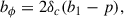
Here, δ_NG is the density field sourced by the potential Φ_NG (Eq. (1)), b₁ is a linear bias that relates the overdensity of halos to that of matter, and b_ϕ is the PNG bias, degenerated with f_NL. A typical parameterization of b_ϕ is

$$\begin{array}{c}\hfill b_{\varphi }=2{\delta }_c(b_1-p),\end{array}$$(3)

where δ_c = 1.69 is the critical density threshold for spherical collapse, and p describes halo formation in primordial overdensities (Barreira 2020). We assume the universality relation p = 1, which is consistent with our halo mass cut (see Sect. 5.1 and Gutiérrez Adame et al. 2024).

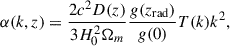
The scale-dependent factor, α, is a function of the wave number, k, associated with density perturbations on scales of s ∼ k⁻¹ and at the redshift z:

$$\begin{array}{c}\hfill \alpha (k,z)=\frac{2c^{2}D(z)}{3H_0^2{\mathrm{\Omega }}_m}\frac{g(z_{\mathrm{rad}})}{g(0)}T(k)k^2,\end{array}$$(4)

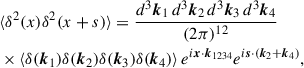
where c is the speed of light, Ω_m is the present day relative matter density, and D(z) is the growth factor normalized to 1 at z = 0. The factor g(z_rad)/g(0) takes into account the difference of this normalization with respect to the early time matter-dominated epoch. The transfer function T(k) is close to unity for scales s > L₀ = 16(Ω_m, 0h²)⁻¹ ≈ 3 h⁻¹ Mpc, which are typically considered in LSS clustering analyses. Thus, the PNG-generated density perturbations depend quadratically on the scale s.

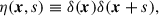
To probe the imprint of these scale-dependent, non-Gaussian features on the LSS, we computed the correlation of the matter perturbation field:

$$\begin{array}{c}\hfill \eta (\mathit{x},s)\equiv \delta (\mathit{x})\delta (\mathit{x}+s),\end{array}$$(5)

where bold variables represent three-dimensional vectors. Note that in this notation, the standard two-point correlation function corresponds to the spatial average of η–that is, the average over all pairs of points separated by a distance, s:

$$\begin{array}{c}\hfill {\xi }_2(s)\equiv ⟨\eta (\mathit{x},s)⟩.\end{array}$$(6)

2.2. Evaluation of matter density field

The matter density field in simulations and real data is evaluated on a discrete grid. In this setting, the density-contrast product from Eq. (5) becomes a discrete convolution:

$$\begin{array}{c}\hfill \eta (\mathit{x},s)=\delta (\mathit{x})[\delta (\mathit{x})\ast \ast \ast K(s)],\end{array}$$(7)

where K(s) is a spherical shell kernel of radius s and thickness Δs, and * * * denotes a 3D discrete convolution.

We computed this quantity using the ConKer algorithm (Brown et al. 2022), which operates on the density-contrast grid:

$$\begin{array}{c}\hfill W_0(X,Y,Z)\equiv D(X,Y,Z)-R(X,Y,Z),\end{array}$$(8)

where D(X, Y, Z) and R(X, Y, Z) represent the data and random tracer counts in the cell (X, Y, Z), respectively, and the full catalog is divided into N such cells.

Next, we convolved W₀ with spherical kernels across a range of scales s = 55 h⁻¹ Mpc − 395 h⁻¹ Mpc, in bins of width Δs = 20 h⁻¹ Mpc. For our actual test cases, the maximum scale, s, we use may vary; see Sect. 3.1, Appendix C for justification. This procedure yields a histogram grid at each scale:

$$\begin{array}{c}\hfill W_1(X,Y,Z;s)\equiv W_0(X,Y,Z)\ast \ast \ast K(s),\end{array}$$(9)

as illustrated in Fig. 1.

Fig. 1. Two-dimensional schematic of how ConKer algorithm evaluates density field with W0 and W1. This shows the convolution of the matter-density variation field, W0 = D − R (left), with a spherical shell kernel, K, with a radius of s and width of Δs. The resulting product is the density histogram, W1 (right). In this example, the inner product is eight, which is placed in the center cell of the W1 grid. The kernel center iterates over each cell, performing this convolution at each scale s.

We applied the same procedure to the random catalog to compute

$$\begin{array}{c}\hfill B_1(X,Y,Z;s)\equiv B_0(X,Y,Z)\ast \ast \ast K(s),\end{array}$$(10)

where B₀ is just the random catalog tracer counts R(X, Y, Z). In this notation, δ(x)∼W₀(X, Y, Z) and δ(x)* * *K(s)∼W₁(X, Y, Z; s), so the discrete density-contrast product from Eq. (7) becomes

$$\begin{array}{c}\hfill \eta \mathbf{(}X,Y,Z;s)=W_0(X,Y,Z)·W_1(X,Y,Z;s).\end{array}$$(11)

To construct a scalar field suitable for moment analysis, we flattened η(X, Y, Z; s) into a one-dimensional array and normalized it using the spatial average-random-field product, ⟨η_R(s)⟩, yielding

$$\begin{array}{c}\hfill {\mathrm{\Gamma }}_n(s)\equiv \frac{\eta (X,Y,Z;s)}{⟨{\eta }_R(s)⟩}\frac{N_R^2}{N_D^2},\end{array}$$(12)

where n indexes over the flattened spatial grid, and N_D and N_R are the total counts of data and random tracers, respectively. This normalization mitigates boundary artifacts arising from the absence of periodic boundary conditions in the ConKer algorithm and ensures consistent statistics across simulations.

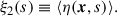
The resulting Γ_n(s) distributions encode scale-dependent deviations from Gaussianity. As seen in Fig. 2, these deviations manifest themselves as variations in the shape (particularly the width and skewness) of the distributions on different scales, characterized by the value of f_NL. This behavior underscores the sensitivity of Γ_n(s) to PNG. This motivated our next step: quantifying these deviations by computing the Gaussian moments (referred to as moments for brevity) of the distributions, which provide a compact and statistically robust characterization of the underlying PNG.

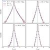Fig. 2. Distributions of flattened density-perturbation estimator, Γn(s), averaged over all 125 FastPM-L1 simulations, shown at s = 95, 195, 295, and 395 h−1 Mpc for the fNL = −25 (blue), 0 (black), and 25 (red) cases.

2.3. Density perturbation moments

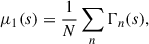
To probe non-Gaussian features in the matter density field, we computed the first three moments of the flattened distributions, Γ_n(s). This is motivated by the fact that information about a distribution’s shape is fully encoded in a series expansion of its moments. The first moment, μ₁(s), is equivalent to the mean (analogous to the 2pcf; see Sect. 4.2), the second, μ₂(s), is the variance, and the third, μ₃(s), is the skewness of the distribution:

$$\begin{array}{cc}\hfill {\mu }_1(s)& =\frac{1}{N}{\displaystyle \sum _n}{\mathrm{\Gamma }}_n(s),\hfill \end{array}$$(13)

$$\begin{array}{cc}\hfill {\mu }_2(s)& =\frac{1}{N}{\displaystyle \sum _n}{[{\mathrm{\Gamma }}_n(s)-{\mu }_1(s)]}^2,\hfill \end{array}$$(14)

$$\begin{array}{cc}\hfill {\mu }_3(s)& =\frac{1}{N}{\displaystyle \sum _n}{[{\mathrm{\Gamma }}_n(s)-{\mu }_1(s)]}^3,\hfill \end{array}$$(15)

where the summations are taken over the N spatial grid points in the density perturbation estimator (see Appendix A for a deeper, physical interpretation of the density moments).

These three moments cumulatively characterize the central tendency, spread, and asymmetry of the distribution. Since a function is fully encoded in its infinite series of moments, even a truncated expansion can efficiently capture deviations from Gaussianity.

As illustrated in Fig. 3, these functions have a noticeable dependence on the f_NL parameter, with the moments from the positive (negative) f_NL case having greater (lesser) magnitudes than those for the fiducial f_NL = 0 case. More specifically, since W₀ ∼ δ, and δ varies linearly with f_NL from Eq. (2), we expect the density grids, W, to exhibit this same dependence. Therefore, given that our density perturbation-estimator, Γ_n(s), includes a product of these density fields in the form of Eq. (11), we expect the moments to exhibit a quadratic dependence in f_NL (see Fig. 4 and Eq. (17)). So, in constructing a combined vector of these moments, we obtained a tool sensitive to PNG. We note that this dependence is only complete for μ₁; higher moments include higher powers of Γ_n(s) and thus higher order terms in f_NL (f_NL⁴ and f_NL⁶ for the second and third moments, respectively; see Sect. 5 for further comments). In practice, however, we find that quadratic parameterization is sufficient for the range of scales considered in this analysis.

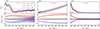Fig. 3. Moments μ1, μ2, and μ3 (left to right) computed from average density fields of the 125 FastPM-L1 simulations, shown for fNL = −25 (blue), 0 (black), and 25 (red). Top panels show raw values; bottom panels show residuals relative to the fNL = 0 case. Shaded regions represent the standard error across simulations. All moments are scaled by s2 to highlight LSS.

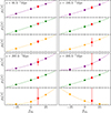Fig. 4. First (purple), second (green), and third (orange) moments plotted as a function of fNL for the same s bins as in Fig. 2. Each point represents the average moment computed from the 125 FastPM-L1 simulations at fNL = −25, 0, and 25, comprising the observation vector, ${\widehat{\mu }}_i$ (with each moment plotted separately). Dashed lines indicate the quadratic fit; i.e., the expectation vector ${\stackrel{\sim }{\mu }}_i(f_{\text{NL}})$. The fNL = 12 test case is shown as a red star, with error bars representing the standard error on μ across the 125 simulations.

We concatenated the three moments into a single observation vector:

$$\begin{array}{c}\hfill {\widehat{\mu }}_i=[{\mu }_1(s),{\mu }_2(s),{\mu }_3(s)],\end{array}$$(16)

with i indexes over s bins. For 18 bins per moment, this yields a total of 3 × 18 = 54 elements in the vector. As we demonstrated, each individual moment follows a roughly quadratic dependence on f_NL, so we expect the full observation vector to exhibit similar behavior. Accordingly, for a catalog with arbitrarily seeded PNG, we modeled the expectation vector as

$$\begin{array}{c}\hfill {\stackrel{\sim }{\mu }}_i(f_{\text{NL}})={\mathcal{A}}_i{f}_{\text{NL}}^2+{\mathcal{B}}_i{f}_{\text{NL}}+{\mathcal{C}}_i,\end{array}$$(17)

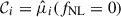where ${\mathcal{C}}_i={\widehat{\mu }}_i(f_{\text{NL}}=0)$. The coefficients 𝒜_i and ℬ_i encode the expected scale-dependent response of each moment to PNG and are determined from fits to multiple simulations with known values of f_NL.

3. Application to simulations

3.1. Simulations

Approximately 80% of the matter in the Universe is believed to be composed of DM, which forms massive, gravitationally bound structures called halos–within which galaxies form. By simulating a Universe composed entirely of DM particles, we can effectively emulate its large-scale structure (see Eq. (2)).

For this study, we used a suite of four approximated particle-mesh N-body simulations generated with FastPM (Feng et al. 2016), each seeded with local PNG values of f_NL = −25, 0, 12, and 25 (see run-knl-3 in Chaussidon 2023). The non-Gaussian initial conditions (via Eq. (1)) are imposed at redshift z = 19, and the simulations are evolved to z = 1.5, covering a volume of (L = 5.52 h⁻¹ Gpc)³ with particle masses of ∼10¹¹ h⁻¹ M_⊙. This redshift is imposed for our study, as it is the only snapshot available in the simulation suite. Moreover, z = 1.5 lies near the median redshift of quasars (QSOs) and close to the upper end of the emission-line galaxy (ELG) and luminous red galaxy (LRG) samples targeted by current and upcoming surveys such as the Dark Energy Spectroscopic Instrument (DESI) (e.g., Prada et al. 2025), making it well suited for demonstrating our method.

Each simulation volume is divided into N_m = 125 non-overlapping sub-boxes of (L = 1 h⁻¹ Gpc)³, which we refer to as the FastPM-L1 simulations (the remaining 0.52 h⁻¹ Gpc is discarded). This subdivision into “mini-universes” is justified by the cosmological assumption of homogeneity and enables us to compute a covariance matrix (see Eq. (21)) from 125 independent mock realizations per f_NL (see Sect. 5.2 for caveats).

To ensure a consistent tracer population and preserve the universality relation (p = 1; see Gutiérrez Adame et al. 2024 and Sect. 5.1), we applied a minimum halo mass cut of M_h > 5 × 10¹² h⁻¹ M_⊙, yielding N_D ≈ 5.5 × 10⁵ halos per box. The resulting comoving halo number density, n ≃ 5.5 × 10⁻⁴ h³ Mpc⁻³, is comparable to the tracer densities of modern, large-scale galaxy-redshift surveys. In DESI, for example, this is similar to LRGs (n ∼ 3 − 6 × 10⁻⁴ h³ Mpc⁻³) and somewhat below ELGs (n ∼ 10⁻³ h³ Mpc⁻³), while being significantly higher than QSOs (n ∼ 10⁻⁵ h³ Mpc⁻³) (Prada et al. 2025). A corresponding random catalog was generated by populating a (L = 1 h⁻¹ Gpc)³ box with N_R = 10N_D randomly distributed objects.

We used the f_NL = −25, 0, and 25 simulations to build our model, reserving the f_NL = 12 simulations for validation. From each box, we evaluated the scale-dependent density perturbation field Γ_n(s) as described in Sect. 2.2 and computed the average field ⟨Γ_n(s)⟩_m–where m indexes over the N_m = 125 simulations–for each f_NL value. These simulation-averaged distributions form the basis for our moment vectors (see Figs. 2 and 3). Unless otherwise noted, all references to Γ_n(s) refer to these averaged fields. We note that a distinct random catalog was generated per sub-box to preserve statistical independence.

From these averaged fields, we computed the moment vectors ${\widehat{\mu }}_i(f_{\mathrm{NL}})$ using Eq. (16), yielding three sets of observations at f_NL = −25, 0, and 25. We then fit these with a quadratic model (Eq. (17)) to extract the coefficients:

$$\begin{array}{cc}\hfill {\mathcal{A}}_i& =[{\widehat{\mu }}_i(25)+{\widehat{\mu }}_i(-25)-2{\widehat{\mu }}_i(0)]/1250,\hfill \end{array}$$(18)

$$\begin{array}{cc}\hfill {\mathcal{B}}_i& =[{\widehat{\mu }}_i(25)-{\widehat{\mu }}_i(-25)]/50,\hfill \end{array}$$(19)

$$\begin{array}{cc}\hfill {\mathcal{C}}_i& ={\widehat{\mu }}_i(0).\hfill \end{array}$$(20)

These yield the expectation vector ${\stackrel{\sim }{\mu }}_i(f_{\text{NL}})$ used throughout the analysis. Figure 4 shows the fits on selected scales.

3.2. Statistical framework

To evaluate the robustness of our model and assess its sensitivity to PNG, we test it against an independent catalog with known f_NL. First, to characterize uncertainties in our observation vector, we derived a covariance matrix from the N_m = 125 f_NL = 0 simulations:

$$\begin{array}{c}\hfill C_{\mathit{ij}}=\frac{1}{N_m-1}{\displaystyle \sum _m}[{\widehat{\mu }}_{m,i}-{⟨\widehat{\mu }⟩}_i][{\widehat{\mu }}_{m,j}-{⟨\widehat{\mu }⟩}_j],\end{array}$$(21)

where ${\widehat{\mu }}_{m,i}$ is the value of the i-th bin from the m-th simulation, and ${⟨\widehat{\mu }⟩}_i$ is the mean of that bin over all N_m realizations. The index, j, iterates over each bin independently of i, corresponding to the second dimension of the covariance matrix. The covariance matrix structure is shown in Fig. 5, computed from the fiducial f_NL = 0 FastPM-L1 set following standard practice (see Appendix B).

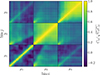Fig. 5. Correlation matrix ($C_{\mathit{ij}}/\sqrt{C_{\mathit{ii}}{C}_{\mathit{jj}}}$) computed from 125 fNL = 0 simulations using Eq. (21). The matrix here was derived using the full observation vector out to smax = 395 h−1 Mpc (54 total bins, 18 per moment). Dashed lines separate the blocks corresponding to different moments in the observation vector, ${\widehat{\mu }}_i$.

Next, we constructed a test statistic to quantify the agreement between the observed vector, ${\widehat{\mu }}_i$, and the expected vector, ${\stackrel{\sim }{\mu }}_i(f_{\text{NL}})$. Assuming a Gaussian likelihood, the χ² statistic is given by

$$\begin{array}{c}\hfill {\chi }^2(f_{\text{NL}})={\displaystyle \sum _{\mathit{ij}}}{[{\widehat{\mu }}_i-{\stackrel{\sim }{\mu }}_i(f_{\text{NL}})]}^T{C}_{\mathit{ij}}^{-1}[{\widehat{\mu }}_j-{\stackrel{\sim }{\mu }}_j(f_{\text{NL}})].\end{array}$$(22)

The best fit, f_NL, was then obtained by minimizing χ² with respect to f_NL for the given observation vector. In Sect. 4, we apply this formalism to the f_NL = 12 FastPM-L1 simulation set and compare the performance of the full moment vector against its individual components.

4. Results: Sensitivity to PNG

4.1. f_NL = 12 test case

To evaluate the sensitivity of our method to PNG, we applied it to a test catalog of 125 FastPM-L1 simulations with f_NL = 12. These simulations were not used to calibrate the f_NL–moment relation, but they lie within the interpolation range of the model (f_NL ∈ [ − 25, 25]), making them ideal for validation.

For this test, we restricted our analysis to a maximum scale of s_max = 275 h⁻¹ Mpc, chosen to optimize reliability given the simulation volume and sample size (see Appendix C). Accordingly, the expectation vector $\stackrel{\sim }{\mu }(f_{\text{NL}})$ (Eq. (17)), observation vector $\widehat{\mu }$ (Eq. (16)), and covariance matrix C_ij (Eq. (21)) are computed using 12 s-bins and the first three moments, yielding a vector of length N = 36 and a 36 × 36 covariance matrix.

As a preliminary check, we show in Fig. 4 the moments from the averaged f_NL = 12 simulations (red stars) at several s-bins alongside the model’s quadratic fit (dashed lines). The close agreement confirms that the test case is well-described by our quadratic moment model, even including scales beyond s_max (shown for illustration).

We then sampled the posterior using the affine-invariant Markov chain Monte Carlo (MCMC) sampler emcee (Foreman-Mackey et al. 2013), based on Goodman and Weare’s algorithm (Goodman & Weare 2010). We used 30 walkers over 10 000 steps, discarding the first 1000 as burn-in and thinning by half the autocorrelation time to retain independent samples. The resulting marginalized posterior on f_NL is shown in Fig. 6, yielding 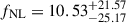$f_{\text{NL}}=10.{53}_{-25.17}^{+21.57}$, which is consistent with the true value of f_NL = 12 within 0.1σ and exhibits only a small bias of Δf_NL = −1.47; this is well within the expected uncertainty given the size of the mock ensemble.

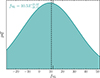Fig. 6. Gaussian fit of marginalized posterior distribution on fNL from MCMC sampling of the fNL = 12 test case. The dashed line marks the median, with uncertainties given by the 16th and 84th percentiles (top left). The true value fNL = 12 is marked with extended ticks on the upper and lower x-axes.

To further assess reliability, we computed the pull statistic:

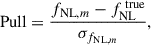$$\begin{array}{c}\hfill \mathrm{Pull}=\frac{f_{\text{NL},m}-f_{\text{NL}}^{\text{true}}}{{\sigma }_{f_{\text{NL},m}}},\end{array}$$(23)

where f_NL, m and σ_fNL, m are the measured value and 1σ uncertainty from the m-th test simulation, and $f_{\text{NL}}^{\text{true}}=12$. For each simulation, we computed ${\widehat{\mu }}_{m,i}$ from the m-th box, derived ${\stackrel{\sim }{\mu }}_i(f_{\text{NL}})$ from the other 124 boxes, and computed the covariance matrix using the remaining 124 f_NL = 0 mocks. This ensures each pull measurement is fully independent of the model. A properly calibrated method should yield a pull distribution with a mean of zero and a standard deviation of one.

The resulting pull distribution is shown in Fig. 7, with mean = −0.20 and std. dev. = 1.31. The slightly broadened distribution reflects the modest simulation count used for the N = 36-bin vector. We fit the pull histogram over the range Pull ∈ [ − 3, 3] to exclude a small number of non-Gaussian tails, which likely stem from sample noise (see Sect. 5.2).

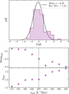Fig. 7. Top panel: Distribution of pull statistic (Eq. (23)) computed from 125 fNL = 12 simulations (purple). A Gaussian fit to the central region (−3 < Pull < 3; dashed line) yields a mean of −0.20 and standard deviation of 1.31. Bottom panel: Mean and standard deviation of pull distribution as a function of smax, the largest radial bin included in the analysis. The dashed vertical line marks the adopted value smax = 275 h−1 Mpc used in the test case.

4.2. Comparison of individual moments

To better understand our model’s sensitivity to PNG and to assess how it compares to the standard two-point correlation function (2pcf), we analyzed the contribution of each individual moment. Specifically, we decomposed the full observation vector, ${\widehat{\mu }}_i$, into its components–μ₁(s), μ₂(s), and μ₃(s)–and evaluated their respective constraining power on f_NL. We also examined the combined moment vector, ${\widehat{\mu }}_i=[{\mu }_1(s),{\mu }_2(s)],$ to test the impact of excluding the third moment.

For each moment combination, we independently fit the expectation vector coefficients 𝒜_i, ℬ_i, and 𝒞_i and constructed the corresponding statistical model as outlined in Sect. 3.2. We then performed MCMC sampling using the same f_NL = 12 simulation set described in Sect. 4.1. The resulting marginalized posteriors are shown in the top panel of Fig. 8.

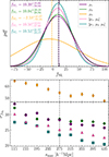Fig. 8. Top panel: Marginalized posterior distributions of fNL for five different observables: μ1 (purple), μ2 (green), μ3 (yellow), [μ1, μ2] (pink), and [μ1, μ2, μ3] (our full model, cyan; see Eq. (16) and Fig. 6). Each observation vector is constructed and sampled independently using the fNL = 12 test simulations. Dashed lines indicate the median value of the MCMC posterior for each case, with corresponding uncertainties (16th and 84th percentiles) annotated in the upper left. Bottom panel: 1σ uncertainty on fNL as function of maximum scale, smax, used in the observation vector. Colors correspond to those in the top panel. Each point represents an independent sampling using bins up to that smax. The dashed vertical gray line marks the smax adopted for the main analysis.

The first and second moments perform similarly, each recovering f_NL within 0.1σ of the true value. The third moment, μ₃(s), has significantly larger uncertainty and bias, recovering f_NL within 0.3σ. Nonetheless, including μ₃(s) in the full vector improves the overall constraint: adding the third moment reduces the uncertainty by ∼8% compared to the [μ₁,  μ₂] case and slightly lowers the bias. This improvement is consistent across a range of maximum scales, as shown in the bottom panel of Fig. 8 (pink points consistently below cyan).

Combining the first two moments alone reduces the uncertainty by ∼13% compared to using either one individually. These results highlight the complementary information each moment provides and support the use of the full three-moment vector to maximize sensitivity to PNG.

To contextualize these gains, we compare our method to the 2pcf. As defined in Eq. (6), the 2pcf is equivalent to the spatial average of η(x, s), which corresponds to the first moment of the density perturbation estimator:

$$\begin{array}{c}\hfill {\mu }_1(s)={⟨{\mathrm{\Gamma }}_n(s)⟩}_n\propto \frac{⟨\eta (X,Y,Z;s)⟩}{⟨{\eta }_R(X,Y,Z;s)⟩}\sim {\xi }_2(s).\end{array}$$(24)

That is, μ₁(s) captures the 2pcf signal normalized by the random correlation field ⟨η_R⟩. Therefore, comparing the full moments method ([μ₁,  μ₂,  μ₃]) to μ₁ alone is effectively a comparison of our moments method with the 2pcf. In this case, we find an ∼21% reduction in the uncertainty on f_NL, indicating a significant sensitivity gain with minimal additional computational cost, since all three moments are derived from the same estimator.

5. Discussion

Leveraging a suite of gigaparsec-scale halo simulations, we demonstrated that a moments-based description of the density field recovers local primordial non-Gaussianity with percent-level accuracy and delivers ∼21% tighter sensitivity to f_NL than the traditional two-point correlation function. Because sharpening f_NL constraints is essential for distinguishing single- from multi-field inflationary models–and thus for decoding the physics of the early Universe–the next challenge is to translate this proof of concept to real survey data. In what follows, we therefore (i) lay out the practical steps needed to incorporate tracer bias and an optimal halo-mass cut, (ii) assess the numerical and volume-related limitations of our present simulation suite, and (iii) highlight the unexpectedly strong constraining power of the second density moment, which points the way to even greater gains.

5.1. Tracer bias and mass cut

The statistical model introduced herein probes the cosmic-matter-density field for evidence of local PNG. Our method performs well in the validation tests described in this work. The primary goal of this study is to lay the groundwork for applying this methodology to observational data, particularly to large datasets with galaxy tracers such as those from DESI. However, several critical steps must be undertaken to adapt the model to such applications. Chief among these is the inclusion of the linear bias, b₁, of the tracer of interest. Since our method is simulation based, any tests performed using survey tracers must account for the difference in magnitude of the PNG signal between the halo simulations used to derive the model and the observed tracer (as the framework described in Equations 15–19 of Brown et al. 2025). While DM halos are a more direct tracer of the LSS, galaxies introduce additional biases arising from selection effects, environmental influences, and population characteristics. Properly accounting for these effects is crucial to decoupling the fiducial halo-mass cut selection, M_h, from the model’s predictions on observational data, thereby enhancing the model’s applicability and robustness.

A second clarification concerns our choice to omit a priori PNG bias measurements and to adopt a mass cut that preserves the universality relation p = 1. In practice, we measured the halo overdensity, δ_h, and the model ties the full expression–including any dependence on the PNG bias, b_ϕ or p–to the known input value of f_NL in the simulation catalogs. Hence, we were only sensitive to the degenerate product f_NL b_ϕ; the calibration absorbs the individual bias factors and renders them irrelevant for the present analysis. We nevertheless imposed a minimum halo mass, M_h, min, chosen to keep p = 1 in the halo-mass function (Gutiérrez Adame et al. 2024). This choice maximizes the separation of the f_NL b_ϕ signal (via Eqs. (2)–(3)) and simplifies the treatment of the scale-dependent bias, reducing potential systematics and sharpening the eventual constraint on f_NL.

5.2. Limitations of our study

Our validation tests draw on four L = 5 h⁻¹ Gpc super–simulations, each sliced into 125 cubic sub–volumes of L = 1 h⁻¹ Gpc. Treating those sub–boxes as independent allowed us to assemble the N_m = 125 mocks used for the covariance matrix and moment uncertainties, but it implicitly assumes statistical homogeneity across the parent box. In real space, that approximation appears largely benign: even a generous convolution kernel of radius s = 500 h⁻¹ Mpc still fits inside a sub–box, and edge effects are mitigated by (i) the integral–constraint correction built into ConKer (Brown et al. 2022) and (ii) the normalization by the mean random density contrast ⟨η_R(s)⟩ (see also Riquelme et al. 2023). In Fourier space, however, each kernel is an average over all wave vectors k; long modes with k ≲ 0.006 h Mpc⁻¹ (comparable to the fundamental mode of a 1 h⁻¹ Gpc box) are shared by adjacent sub–boxes. Consequently, the same super–survey fluctuation feeds multiple “independent” realizations, and the number of truly independent modes drops below unity for scales s ≳ 180 h⁻¹ Mpc (Eq. (A.10)). The result is likely an understatement of large–scale variance and an over-optimistic covariance matrix. Crucially, this caveat reflects our mock construction, not an intrinsic flaw of the moments method; real surveys–or mock suites generated as separate boxes–naturally include the full super-sample covariance matrix.

A related issue is the size of the mock ensemble. The fiducial covariance matrix is 36 × 36, but it is derived from only N_m = 125 mocks, whereas the rule of thumb N_m ≳ 10N would suggest N_m ≳ 360. The widened pull distribution (σ_pull = 1.31; Fig. 7) indicates that statistical noise inflates our error bars. Generating an order-of-magnitude larger ensemble is straightforward–modern surveys routinely provide thousands of low-fidelity mocks for precisely this purpose.

A third systematic concerns the scale range and binning. Our sensitivity to f_NL saturates at the largest kernel radii probed, s_max, which are capped by the catalog volume (Appendix C). Kernels approaching the full (1 h⁻¹ Gpc)³ box become noisy and unreliable. Larger volume data sets such as the DESI DR2 catalog (2.4 h⁻¹ Gpc)³ would admit longer modes, tighten the constraints (see the decreasing trend with s_max in Fig. 8), and support finer binning (e.g., Δs = 4 h⁻¹ Mpc in Abdul Karim et al. 2025, versus our current 20 h⁻¹ Mpc).

Lastly, we revisited our working assumption that the moment vector depends quadratically on f_NL. Section 2.3 shows that each individual moment scales as ${\mu }_n\propto f_{\mathrm{NL}}^{2n}$, so only μ₁ is strictly quadratic; higher moments contain higher order terms that we truncated. This approximation holds up both visually – each moment adheres closely to a quadratic fit across scales (Fig. 4) – and empirically, as the full moment vector delivers strong constraining power (Fig. 6). Residuals only become noticeable for s > 300 h⁻¹ Mpc, where the f_NL = 12 test begins to deviate in μ₃. While a denser simulation grid in f_NL could in principle model these higher order terms, the deviation remains well within our error bars, and both LSS and CMB data already place $f_{\mathrm{NL}}^{\mathrm{loc}}$ comfortably in the [ − 10, 10] range. For these reasons, the quadratic truncation is more than sufficient for our analysis. Future work may explore higher order models for completeness, though we do not expect a meaningful gain in sensitivity.

In short, the dominant systematics – box coupling, limited mock statistics, and volume-driven scale cuts – stem from our test bed rather than from the method itself. All can be alleviated with larger volume, higher multiplicity mock catalogs, and exploring those upgrades is a clear next step.

5.3. Promise of the second moment

Beyond addressing these limitations, our analysis uncovers an unexpected strength: the second moment alone carries nearly as much constraining power as the mean (see Fig. 8). As we show in Sect. 4.2, μ₁ ∼ ξ₂; so, comparing the first and second moments is similar to comparing the familiar 2pcf (the average of the density perturbations) to μ₂ (the variance of the density perturbations). Since both moment vectors contain the same number of bins, this comparison is not confounded by binning resolution or covariance matrix smoothness. Figure 8 confirms that μ₂ offers sensitivity to f_NL comparable to μ₁, while Fig. 3 further shows that μ₂ more clearly tracks the scale-dependent bias, evident in the growing separation between different f_NL cases in the lower center panel. This pattern is also visible in the density-field distributions (Fig. 2), where the mean remains similar across scales, but the width (i.e., μ₂) narrows significantly. Finally, the physical interpretation of μ₂ given in Appendix A suggests that the second (and higher) moment(s) may surpass μ₁ in sensitivity in larger volume surveys. Altogether, these findings point to a promising path: analyses of PNG in the LSS may benefit from combining perturbation moments (or even using the variance alone) – rather than relying solely on mean-based statistics such as the two-point function. This approach is computationally efficient and potentially more sensitive to PNG than the classic 2pcf one.

5.4. Outlook

Looking forward, three incremental yet concrete steps will carry this proof of concept across the finish line to a survey-ready analysis. First, explicitly embedding the tracer’s linear and scale-dependent bias in our forward model – together with a well-motivated lower halo-mass threshold – will disentangle the f_NL imprint from galaxy-selection systematics and extend our calibration beyond DM halos. Second, deriving the covariance matrix from a mock ensemble at least an order of magnitude larger than the present N_m = 125 will quench statistical noise, stabilize large-scale bins, and permit finer radial binning. Third, deploying the method on volumes on the order of (2.4 h⁻¹ Gpc)³–for example, those available in DESI DR2–will admit modes with k ≲ 0.003 h Mpc⁻¹ and further amplify the constraining power, especially in the second and higher moments. Work along these lines is already under way and will be detailed in a forthcoming paper.

6. Conclusions

In this work, we introduced a new framework for probing primordial non-Gaussianity using the moments of the density perturbation field. By computing the first three moments of the normalized two-point estimator, Γ_n(s), from DM-halo simulations seeded with varying f_NL, we built a statistical model that captures the scale-dependent signatures of local PNG. Applying this model to an independent f_NL = 12 test simulation set, we demonstrated percent-level recovery and an ∼21% improvement in sensitivity over the traditional two-point correlation function.

These results highlight the potential of moment-based observables as efficient and powerful summary statistics for LSS analyses. In particular, the second moment alone was shown to carry nearly equivalent constraining power to the mean, suggesting that higher moments can extract additional PNG signal without significant added computational cost.

Future refinements – including the improved treatment of tracer bias, expanded simulation ensembles, and the modeling higher order dependencies in f_NL – will be essential for adapting this method to observational data. As ongoing surveys such as DESI deliver increasingly large and precise catalogs, moment-based analyses offer a scalable path to sharpening constraints on primordial physics and advancing our understanding of the inflationary universe.

Acknowledgments

E.V.’s stipend at SAO is supported through the Chandra X-Ray Center grant GO3-24093X and Space Telescope Science Institute grant HST-GO-17177. Z.B. is grateful for support from the US Department of Energy via grants DE-SC0021165 and DE-SC0011840. R.D. acknowledges support from the Department of Energy under the grant DE-SC0008475.0. E.C. is supported by the Director, Office of Science, Office of High Energy Physics of the U.S. Department of Energy under Contract No. DE-AC02-05CH1123, and by the National Energy Research Scientific Computing Center, a DOE Office of Science User Facility under the same contract.

References

Appendix A: Physical interpretation of higher moments

In Sect. 2.3, we introduced the empirical definitions of the Gaussian moments (Eqs. (13)–(15)). Here, we derived an analytic expression for the second moment, μ₂(s), to clarify its physical meaning and justify its value in constraining PNG. We omitted μ₁ since it corresponds to the usual 2pcf, and μ₃ since its interpretation follows naturally from this treatment.

The second moment–i.e., the variance–is given by

$$\begin{array}{cc}\hfill {\mu }_2(s)& =⟨{(\delta (x)\delta (x+s)-{\mu }_1(s))}^2⟩\hfill \end{array}$$(A.1)

$$\begin{array}{cc}& =⟨{\delta }^2(x){\delta }^2(x+s)⟩-{\mu }_1^2(s).\hfill \end{array}$$(A.2)

The first term encodes the connected four-point function and thus contains the non-Gaussian signal. For simplicity, we omitted the randoms normalization in the above expression, as it does not affect the present discussion. Its Fourier transform is

$$\begin{array}{cc}& ⟨{\delta }^2(x){\delta }^2(x+s)⟩=\frac{d^3{\mathit{k}}_1{d}^3{\mathit{k}}_2{d}^3{\mathit{k}}_3{d}^3{\mathit{k}}_4}{{(2\pi )}^{12}}\hfill \\ \hfill & \times ⟨\delta ({\mathit{k}}_1)\delta ({\mathit{k}}_2)\delta ({\mathit{k}}_3)\delta ({\mathit{k}}_4)⟩e^{i\mathit{x}·{\mathit{k}}_{1234}}{e}^{i\mathit{s}·({\mathit{k}}_2+{\mathit{k}}_4)},\hfill \end{array}$$(A.3)

with k₁₂₃₄ ≡ k₁ + k₂ + k₃ + k₄. This is a collapsed limit of the 4-point function, with two positions at x and two at x + s. While s appears as a vector in the exponential, we averaged over all directions on a sphere of radius |s| to recover the scalar separation s used in the moments.

Applying Wick’s theorem, the 4-point expectation splits into Gaussian and connected parts:

$$\begin{array}{cc}& ⟨\delta ({\mathit{k}}_1)\delta ({\mathit{k}}_2)\delta ({\mathit{k}}_3)\delta ({\mathit{k}}_4)⟩=[⟨\delta ({\mathit{k}}_1)\delta ({\mathit{k}}_2)⟩⟨\delta ({\mathit{k}}_3)\delta ({\mathit{k}}_4)⟩\hfill \\ \hfill & +2\text{permutations}]+{⟨\delta ({\mathit{k}}_1)\delta ({\mathit{k}}_2)\delta ({\mathit{k}}_3)\delta ({\mathit{k}}_4)⟩}_{\text{c}}.\hfill \end{array}$$(A.4)

The Gaussian contractions are already captured in μ₁². The connected component contributes:

$$\begin{array}{c}\hfill {⟨\delta ({\mathit{k}}_1)\delta ({\mathit{k}}_2)\delta ({\mathit{k}}_3)\delta ({\mathit{k}}_4)⟩}_{\text{c}}={(2\pi )}^3{\delta }_D({\mathit{k}}_{1234})\mathcal{T}(k_1,k_2,k_3,k_4),\end{array}$$(A.5)

where 𝒯 is the trispectrum. The Dirac delta enforces momentum conservation and reduces the integral to three independent k-vectors:

$$\begin{array}{cc}& {⟨{\delta }^2(x){\delta }^2(x+s)⟩}_{\text{c}}=\frac{d^3{\mathit{k}}_1{d}^3{\mathit{k}}_2{d}^3{\mathit{k}}_3{d}^3{\mathit{k}}_4}{{(2\pi )}^{12}}{(2\pi )}^3\hfill \\ \hfill & \times {\delta }_D({\mathit{k}}_{1234})\mathcal{T}(k_1,k_2,k_3,k_4)e^{i\mathit{x}·{\mathit{k}}_{1234}}{e}^{i\mathit{s}·({\mathit{k}}_2+{\mathit{k}}_4)}\hfill \end{array}$$(A.6)

$$\begin{array}{cc}& ={\displaystyle \int \int \int \frac{d^3{\mathit{k}}_1{d}^3{\mathit{k}}_2{d}^3{\mathit{k}}_3}{{(2\pi )}^6}}\mathcal{T}(k_1,k_2,k_3,-k_{123})e^{-i\mathit{s}·({\mathit{k}}_1+{\mathit{k}}_3)}.\hfill \end{array}$$(A.7)

This expression emphasizes collapsed configurations (k₁ + k₃ ≈ 0), since the real-space correlator involves only two distinct points. These configurations are especially sensitive to local PNG, which produces long-short mode coupling. The full 4-point function ⟨δ(x₁)δ(x₂)δ(x₃)δ(x₄)⟩_c would span a wider set of shapes (e.g., equilateral, orthogonal), but μ₂ selectively probes the collapsed limit relevant to local-type non-Gaussianity.

A.1. Survey volume sensitivity

This physical picture offers insight into how moment sensitivity scales with volume. In a box of side length L and volume V = L³, the fundamental mode is

$$\begin{array}{c}\hfill {\mathit{k}}_f=\frac{2\pi }{L}\mathit{n},\mathit{n}\in {\mathbb{Z}}^3.\end{array}$$(A.8)

The number of k-modes in a spherical shell of radius k and width Δk is:

$$\begin{array}{c}\hfill N_k(k)=\frac{4\pi k^2\mathrm{\Delta }k}{{(2\pi /L)}^3}=\frac{k^2\mathrm{\Delta }k}{2{\pi }^2}V.\end{array}$$(A.9)

Switching to real-space scale s ∼ 1/k with Δk ≈ Δs/s² yields:

$$\begin{array}{c}\hfill N_k(s)\approx \frac{\mathrm{\Delta }s}{2{\pi }^2{s}^4}V.\end{array}$$(A.10)

So the number of available k-modes falls sharply with increasing s. For example, with V = 1 h⁻³ Gpc³, s = 55h⁻¹ Mpc, and Δs = 20h⁻¹ Mpc, we find N_k ≈ 111–and fewer at larger scales.

Now, since μ₁ samples a single k-vector and μ₂ integrates over three wavevectors (constrained by k₁₂₃₄ = 0), the number of available mode combinations scales as:

$$\begin{array}{cc}\hfill N_k^{{\mu }_1}& \sim N_k,\hfill \end{array}$$(A.11)

$$\begin{array}{cc}\hfill N_k^{{\mu }_2}& \sim N_k^3.\hfill \end{array}$$(A.12)

While the Dirac delta imposes constraints, μ₂ still integrates over a far larger space of configurations than μ₁. This explains its enhanced constraining power in finite-volume surveys and highlights the promise of higher moments for probing PNG. Furthermore, since N_k ∝ V, increases in survey volume significantly enhance the relative signal of higher moments.

Appendix B: Dependence of the covariance matrix on f_NL

In this study, we computed the covariance matrix using the fiducial f_NL = 0 FastPM-L1 simulations, following standard practice in similar analyses (e.g., Mueller et al. 2019, 2022; Adame et al. 2025; Rezaie et al. 2021). To assess the robustness of this assumption, we compared the fiducial covariance matrix with those derived from the f_NL = −25 and f_NL = 25 FastPM-L1 simulations. The relative differences in the normalized covariance matrices are shown in Fig. B.1.

We observed statistically significant deviations between the covariance matrices. In particular, relative differences reach 𝒪(1) in some regions and average around 𝒪(0.1) across the matrix. Notably, the f_NL = −25 and f_NL = 25 covariance matrices seem to diverge from the fiducial case in opposite directions (illustrated by the nearly inverted colors across the 0-point in Fig. B.1).

These results suggest a non-negligible dependence of the covariance matrix structure on the sign and magnitude of the primordial non-Gaussianity with which the simulations are seeded. Since our method probes PNG directly, this dependence suggests a potentially similar impact on other PNG-sensitive observables, such as higher-order n-point correlation functions or the bispectrum. Future studies might explore alternatives such as deriving the covariance matrix from lnP_m, where P_m is the matter power spectrum, which has been shown to exhibit approximate independence from f_NL (see Eq. 13 of Ross et al. 2013).

Fig. B.1. The relative difference between the correlation matrix ($\stackrel{\sim }{C_{\mathit{ij}}}=C_{\mathit{ij}}/\sqrt{C_{\mathit{ii}}{C}_{\mathit{jj}}}$) derived from the fNL = −25 (left) and fNL = 25 (right) simulations, and that from the fNL = 0 fiducial simulations.

Appendix C: Scale dependence

Here we analyzed the scale dependence of our model and justified the choice of s_max = 275h⁻¹ Mpc and bin size Δs = 20h⁻¹ Mpc for constructing the observation vector. While PNG signals grow stronger on large scales due to long-short mode coupling, our simulation boxes span only L = 1h⁻¹ Gpc, so spherical kernels with s ≳ 500h⁻¹ Mpc intersect box boundaries and yield noisy measurements. To avoid this, we limited our tests to s_max ≤ 435h⁻¹ Mpc, maintaining a conservative buffer from the edges.

To determine the optimal s_max, we ran our statistical pipeline at nine values between 115 and 435h⁻¹ Mpc, measuring f_NL and its uncertainty at each. As shown in the bottom panel of Fig. 8, larger s_max yields tighter constraints, as expected. However, increasing the number of bins also enlarges the covariance matrix, worsening its condition given the limited number of simulations (see Sect. 5.2).

To quantify this trade-off, we performed a pull analysis at each s_max (bottom panel of Fig. 7). We found that pulls become increasingly biased and their uncertainties increasingly underestimated at large scales: Mean_pull drifts negative, and σ_pull > 1. As shown in the bottom panel of Fig. 7, both metrics are stable in the range 195–275h⁻¹ Mpc: the bias remains moderate (Mean_pull ≈ −0.1 to −0.2), and the spread stays relatively stable (σ_pull ≈ 1.3). Beyond s_max = 275h⁻¹ Mpc, the pull distribution becomes increasingly skewed and its variance grows rapidly. This plateau identifies 275h⁻¹ Mpc as the upper limit beyond which instability dominates. We therefore adopted s_max = 275h⁻¹ Mpc for testing, as it balances information gain from large-scale modes with robustness of the statistical estimator.

The bin width Δs = 20h⁻¹ Mpc (yielding 36 bins) was chosen similarly. Finer binning increases vector dimensionality and amplifies noise in the covariance matrix, degrading diagnostics like the pull test. We found that moderate variations around Δs = 20 have negligible impact on PNG sensitivity but reduce numerical stability. Thus, the chosen pair (s_max,  Δs) = (275h⁻¹ Mpc,  20h⁻¹ Mpc) reflects a practical minimum in statistical uncertainty and numerical noise given our simulation suite.

All Figures

Fig. 1. Two-dimensional schematic of how ConKer algorithm evaluates density field with W0 and W1. This shows the convolution of the matter-density variation field, W0 = D − R (left), with a spherical shell kernel, K, with a radius of s and width of Δs. The resulting product is the density histogram, W1 (right). In this example, the inner product is eight, which is placed in the center cell of the W1 grid. The kernel center iterates over each cell, performing this convolution at each scale s.

In the text

	Fig. 2. Distributions of flattened density-perturbation estimator, Γn(s), averaged over all 125 FastPM-L1 simulations, shown at s = 95, 195, 295, and 395 h−1 Mpc for the fNL = −25 (blue), 0 (black), and 25 (red) cases.
In the text

	Fig. 3. Moments μ1, μ2, and μ3 (left to right) computed from average density fields of the 125 FastPM-L1 simulations, shown for fNL = −25 (blue), 0 (black), and 25 (red). Top panels show raw values; bottom panels show residuals relative to the fNL = 0 case. Shaded regions represent the standard error across simulations. All moments are scaled by s2 to highlight LSS.
In the text

Fig. 4. First (purple), second (green), and third (orange) moments plotted as a function of fNL for the same s bins as in Fig. 2. Each point represents the average moment computed from the 125 FastPM-L1 simulations at fNL = −25, 0, and 25, comprising the observation vector, ${\widehat{\mu }}_i$ (with each moment plotted separately). Dashed lines indicate the quadratic fit; i.e., the expectation vector ${\stackrel{\sim }{\mu }}_i(f_{\text{NL}})$. The fNL = 12 test case is shown as a red star, with error bars representing the standard error on μ across the 125 simulations.

In the text

	Fig. 5. Correlation matrix ($C_{\mathit{ij}}/\sqrt{C_{\mathit{ii}}{C}_{\mathit{jj}}}$) computed from 125 fNL = 0 simulations using Eq. (21). The matrix here was derived using the full observation vector out to smax = 395 h−1 Mpc (54 total bins, 18 per moment). Dashed lines separate the blocks corresponding to different moments in the observation vector, ${\widehat{\mu }}_i$.
In the text

	Fig. 6. Gaussian fit of marginalized posterior distribution on fNL from MCMC sampling of the fNL = 12 test case. The dashed line marks the median, with uncertainties given by the 16th and 84th percentiles (top left). The true value fNL = 12 is marked with extended ticks on the upper and lower x-axes.
In the text

Fig. 7. Top panel: Distribution of pull statistic (Eq. (23)) computed from 125 fNL = 12 simulations (purple). A Gaussian fit to the central region (−3 < Pull < 3; dashed line) yields a mean of −0.20 and standard deviation of 1.31. Bottom panel: Mean and standard deviation of pull distribution as a function of smax, the largest radial bin included in the analysis. The dashed vertical line marks the adopted value smax = 275 h−1 Mpc used in the test case.

In the text

Fig. 8. Top panel: Marginalized posterior distributions of fNL for five different observables: μ1 (purple), μ2 (green), μ3 (yellow), [μ1, μ2] (pink), and [μ1, μ2, μ3] (our full model, cyan; see Eq. (16) and Fig. 6). Each observation vector is constructed and sampled independently using the fNL = 12 test simulations. Dashed lines indicate the median value of the MCMC posterior for each case, with corresponding uncertainties (16th and 84th percentiles) annotated in the upper left. Bottom panel: 1σ uncertainty on fNL as function of maximum scale, smax, used in the observation vector. Colors correspond to those in the top panel. Each point represents an independent sampling using bins up to that smax. The dashed vertical gray line marks the smax adopted for the main analysis.

In the text

	Fig. B.1. The relative difference between the correlation matrix ($\stackrel{\sim }{C_{\mathit{ij}}}=C_{\mathit{ij}}/\sqrt{C_{\mathit{ii}}{C}_{\mathit{jj}}}$) derived from the fNL = −25 (left) and fNL = 25 (right) simulations, and that from the fNL = 0 fiducial simulations.
In the text

References

- Abdul Karim, M., Aguilar, J., Ahlen, S., et al. 2025, Phys. Rev. D, 112, 083515 [Google Scholar]
- Adame, A. G., Aguilar, J., Ahlen, S., et al. 2025, JCAP, 2025, 012 [Google Scholar]
- Albrecht, A., & Steinhardt, P. J. 1982, Phys. Rev. Lett., 48, 1220 [Google Scholar]
- Andrews, A., Jasche, J., Lavaux, G., et al. 2024, arXiv e-prints [arXiv:2412.11945] [Google Scholar]
- Barreira, A. 2020, JCAP, 2020, 031 [CrossRef] [Google Scholar]
- Brown, Z., Mishtaku, G., & Demina, R. 2022, A&A, 667, A129 [NASA ADS] [CrossRef] [EDP Sciences] [Google Scholar]
- Brown, Z., Demina, R., Adame, A. G., et al. 2025, MNRAS, 543, 2078 [Google Scholar]
- Cagliari, M. S., Barberi-Squarotti, M., Pardede, K., Castorina, E., & D’Amico, G. 2025, JCAP, 07, 043 [Google Scholar]
- Castorina, E., Hand, N., Seljak, U., et al. 2019, JCAP, 2019, 010 [Google Scholar]
- Chaussidon, E. 2023, Theses, Université Paris-Saclay [Google Scholar]
- Chaussidon, E., Yèche, C., de Mattia, A., et al. 2025, JCAP, 2025, 029 [Google Scholar]
- Creminelli, P., D’Amico, G., Musso, M., & Noreña, J. 2011, JCAP, 2011, 038 [Google Scholar]
- Dalal, N., Doré, O., Huterer, D., & Shirokov, A. 2008, Phys. Rev. D, 77, 123514 [CrossRef] [Google Scholar]
- Feng, Y., Chu, M.-Y., Seljak, U., & McDonald, P. 2016, MNRAS, 463, 2273 [NASA ADS] [CrossRef] [Google Scholar]
- Foreman-Mackey, D., Hogg, D. W., Lang, D., & Goodman, J. 2013, PASP, 125, 306 [Google Scholar]
- Gangui, A., Lucchin, F., Matarrese, S., & Mollerach, S. 1994, ApJ, 430, 447 [Google Scholar]
- Goodman, J., & Weare, J. 2010, Commun. Appl. Math. Comput. Sci., 5, 65 [Google Scholar]
- Guth, A. H. 1981, Phys. Rev. D, 23, 347 [Google Scholar]
- Gutiérrez Adame, A., Avila, S., Gonzalez-Perez, V., et al. 2024, A&A, 689, A69 [NASA ADS] [CrossRef] [EDP Sciences] [Google Scholar]
- Kalaja, A., Meerburg, P. D., Pimentel, G. L., & Coulton, W. R. 2021, JCAP, 2021, 050 [CrossRef] [Google Scholar]
- Komatsu, E., & Spergel, D. N. 2001, Phys. Rev. D, 63, 063002 [NASA ADS] [CrossRef] [Google Scholar]
- Linde, A. D. 1982, Phys. Lett. B, 108, 389 [Google Scholar]
- Maldacena, J. 2003, J. High Energy Phys., 2003, 013 [CrossRef] [Google Scholar]
- Mao, Q., Berlind, A. A., McBride, C. K., et al. 2014, MNRAS, 443, 1402 [Google Scholar]
- Mueller, E.-M., Percival, W. J., & Ruggeri, R. 2019, MNRAS, 485, 4160 [Google Scholar]
- Mueller, E.-M., Rezaie, M., Percival, W. J., et al. 2022, MNRAS, 514, 3396 [NASA ADS] [CrossRef] [Google Scholar]
- Novaes, C. P., Thiele, L., Armijo, J., et al. 2025, Phys. Rev. D, 111, 083510 [Google Scholar]
- Planck Collaboration IX. 2020, A&A, 641, A9 [Google Scholar]
- Prada, F., Ereza, J., Smith, A., et al. 2025, A&A, 698, A170 [NASA ADS] [CrossRef] [EDP Sciences] [Google Scholar]
- Rezaie, M., Ross, A. J., Seo, H.-J., et al. 2021, MNRAS, 506, 3439 [Google Scholar]
- Riquelme, W., Avila, S., García-Bellido, J., et al. 2023, MNRAS, 523, 603 [NASA ADS] [CrossRef] [Google Scholar]
- Ross, A. J., Percival, W. J., Carnero, A., et al. 2013, MNRAS, 428, 1116 [NASA ADS] [CrossRef] [Google Scholar]
- Wang, Y., & He, P. 2025, Phys. Rev. D, 111, L041302 [Google Scholar]