| Issue |
A&A
Volume 704, December 2025
|
|
|---|---|---|
| Article Number | A275 | |
| Number of page(s) | 17 | |
| Section | Galactic structure, stellar clusters and populations | |
| DOI | https://doi.org/10.1051/0004-6361/202557051 | |
| Published online | 19 December 2025 | |
Modelling the Milky Way’s exoplanet population based on cosmological galaxy simulations
1
Departament de Física Quàntica i Astrofísica (FQA), Universitat de Barcelona (UB),
Martí i Franquès 1,
08028
Barcelona,
Spain
2
Institut de Ciències del Cosmos (ICCUB), Universitat de Barcelona (UB),
Martí i Franquès 1,
08028
Barcelona,
Spain
3
Institut d’Estudis Espacials de Catalunya (IEEC), Edifici RDIT, Campus UPC,
08860
Castelldefels (Barcelona),
Spain
4
Observatori Fabra, Reial Acadèmia de Ciències i Arts de Barcelona,
Rambla dels Estudis, 115,
08002
Barcelona,
Spain
5
Department of Astronomy, School of Physics and Astronomy, Shanghai Jiao Tong University,
800 Dongchuan Road,
Shanghai
200240,
China
6
State Key Laboratory of Dark Matter Physics, School of Physics and Astronomy, Shanghai Jiao Tong University,
Shanghai
200240,
China
7
Observatório Nacional, MCTI,
Rua Gal. José Cristino 77,
Rio de Janeiro
20921-400,
RJ,
Brasil
8
Institute of Astronomy, University of Cambridge,
Madingley Road,
Cambridge
CB3 0HA,
UK
9
Universidade Federal de Sergipe,
Av. Marechal Rondon, S/N,
49000-000
São Cristóvão,
SE,
Brazil
10
Mullard Space Science Laboratory, University College London,
Holmbury St. Mary,
Dorking,
Surrey
RH5 6NT,
UK
11
National Astronomical Observatory of Japan,
2-21-1 Osawa,
Mitaka,
Tokyo
181-8588,
Japan
12
Laboratòrio Nacional de Astrofísica,
Rua Estados Unidos 154,
37504-364
Itajubá,
MG,
Brazil
13
Instituto Nacional de Pesquisas Espaciais/MCTI,
Av. dos Astronautas 1758,
São José dos Campos,
SP,
Brazil
★ Corresponding author: This email address is being protected from spambots. You need JavaScript enabled to view it.
Received:
31
August
2025
Accepted:
13
November
2025
Abstract
Context. Exoplanet transit and radial-velocity surveys have allowed us to explore the exoplanet population in our Galactic surroundings. The planet populations in more remote areas of the Milky Way (MW) will become accessible with future instrumentation.
Aims. In this paper, we aim to simulate realistic exoplanet populations across different regions of the MW by combining state-of-the-art cosmological simulations of our Galaxy with exoplanet formation models and observations.
Methods. We model the exoplanet populations around simulated single stars, using planet occurrence rate and multiplicity depending on stellar mass, metallicity, and planet type, and assign them physical parameters such as mass and orbital period.
Results. Focussing first on the solar vicinity, we find mostly metallicity-driven differences in the distributions of non-hosting and planet-hosting single stars. In our simulated solar neighbourhood, 52.5% of all planets are Earth-like (23% of them located in the Habitable Zone), 44% are super-Earths or Neptunes, and 3.5% are giant planets. A detailed comparison with the census of Kepler exoplanets and candidates shows that, when taking into account the most relevant selection effects, we obtain a similar distribution of exoplanets compared to the observed population. However, we also detect some significant differences in the exoplanet and host star distributions (e.g. more planets around F-type and red-giant stars compared to the observations) that we attribute mostly to a too strong recent star formation and a too large disc scale height in the simulation compared to the solar neighbourhood, as well as to some caveats in our exoplanet population synthesis that will be addressed in future work. Extending our analysis to other regions of the simulated MW and to other galaxies within the same suite of simulations, we find that the relative percentages of Earth-like, super-Earth or Neptunes, and giant planets remain largely consistent as long as the simulated galaxy matches the morphology and mass of the MW.
Conclusions. We have created a fast and flexible framework to produce exoplanet populations based on MW-like simulations that can easily be adapted to produce predictions for the yields of future exoplanet detection missions.
Key words: planets and satellites: general / planetary systems / Galaxy: disk / Galaxy: evolution / solar neighborhood / Galaxy: stellar content
© The Authors 2025
 Open Access article, published by EDP Sciences, under the terms of the Creative Commons Attribution License (https://creativecommons.org/licenses/by/4.0), which permits unrestricted use, distribution, and reproduction in any medium, provided the original work is properly cited.
This article is published in open access under the Subscribe to Open model. This email address is being protected from spambots. You need JavaScript enabled to view it. to support open access publication.
1 Introduction
The discovery, exploration, and study of exoplanets have started a new era in astrophysics. After 30 years of discoveries, the field of exoplanetary science has reached remarkable advancements in recent years through innovative observation techniques, including better precision in radial velocity measurements, transmission spectroscopy, or direct imaging. As of February 2025, 5823 exoplanets have been confirmed1 (Christiansen et al. 2025).
Several space missions have already explored the exoplanet population in our Galactic surroundings. The most successful surveys so far have been the Kepler Space Telescope (Borucki et al. 2010) and its follow-up mission K2 (Howell et al. 2014), which already account for more than half of the currently confirmed exoplanets (Lissauer et al. 2024, Mayo et al. 2018), the Transiting Exoplanet Survey Satellite (TESS; Pál et al. 2018), and the CoRoT mission Baglin et al. 2006; Deleuil et al. 2018. Presently, the progressive processing of the Gaia mission data (Gaia Collaboration 2016, 2023) is yielding more and more astrometric detections of exoplanets (e.g. Holl et al. 2023; Sahlmann & Gómez 2025), ESA’s CHaracterising ExOPlanet Satellite (CHEOPS, Rando et al. 2018; Fortier et al. 2024) is characterising known exoplanets and their host stars, while the NASA flagship mission James Webb space telescope (JWST, McElwain et al. 2023) is already carrying out transmission spectroscopy of possibly habitable Earth-like exoplanets (e.g. Ahrer et al. 2023). The Planetary Transits and Oscillations of stars mission (PLATO; Rauer et al. 2014, 2025) and Ariel (Atmospheric Remote-sensing Infrared Exoplanet Large-survey; Tinetti et al. 2022) are next-generation telescopes that will provide crucial new statistics on the frequency of different types of exoplanetary systems around different types of stars.
None of the exoplanetary systems discovered to date resemble our Solar System, with almost 80% of the confirmed exoplanet2 with measured mass being heavier than 10 Mθ, while half of the Solar System is composed of small planets. This may be explained by the limitations of the current instruments (in particular, transits and radial-velocity surveys), which tend to favour the detection of massive, short-period planets. Current surveys that account for these selection biases indicate that small planets are more common than giant planets (Johnson et al. 2010; Dressing & Charbonneau 2013; Burke et al. 2015; Bryson et al. 2021). To compensate for the observational biases, various studies tried to derive the probability of a star to host exoplanets (i.e. the occurrence rate), depending on the exoplanet type and the star’s properties, mainly the stellar mass and metallicity (see Pan et al. 2025 and references therein). For example, the occurrence rate of giant planets depends on various variables: it tends to increase with longer orbital periods, as well as with the host star’s metallicity and mass (e.g. Fischer & Valenti 2005; Petigura et al. 2018). It is also observed that multiplanetary systems with resonant orbits and size similarities are common and that exoplanets can form and survive in multiple stellar systems (e.g. Cochran et al. 1997; Anglada-Escudé et al. 2016; Weiss et al. 2018; Triaud et al. 2022).
This work aims to simulate a simple but realistic exoplanet population by modelling the main known factors that influence the existence and distribution of different types of exoplanets. We start from a cosmological simulation of a Milky Way-like galaxy, transform star-particles into stars using stellar evolutionary models, and then generate a synthetic exoplanet population by joining observational results with predictions from exoplanet formation models. Our predictions can thus provide a benchmark for future exoplanet detection missions such as PLATO, HAYDN (High-precision AsteroseismologY in DeNse stellar fields; Miglio et al. 2024), or the Roman Space Telescope’s Galactic Bulge Time Domain Survey (Wilson et al. 2023).
Our paper is structured as follows: in Sect. 2 we describe our method of creating stellar and exoplanetary populations from cosmological galaxy simulations. In Sect. 3, we present the results for a volume-complete exoplanet census of the solar vicinity in our fiducial simulation. In Sect. 4 we compare our model with observations from Kepler using a detailed forward simulation that includes the most relevant selection effects. Sect. 5 then extends our modelling to different environments in the same galaxy, while Sect. 6 studies the differences among the simulated solar-neighbourhood exoplanet populations in six simulated galaxies. In Sect. 7 we summarise and discuss our results in light of the existing literature, and discuss possible future applications and improvements.
2 Methodology
In this work, we aim to simulate a realistic population of exoplanets, starting from a Milky Way-like cosmological galaxy simulation. The star particles used to simulate the initial population of host stars are extracted from a well-tested and publicly available snapshot of a high-resolution cosmological simulation (Sect. 2.1). Focussing on a similar environment to our Solar System in terms of location in the Milky Way, we generate stellar systems from the stellar particles of the host simulation, using a set of stellar models, initial mass function, and multiplicity statistics (Sect. 2.2). Finally, we create planets around these synthetic stars using a series of prescriptions inspired by both the observed exoplanet census and planet population synthesis models (Sect. 2.3).
2.1 Cosmological simulation and solar neighbourhood
We used Numerical Investigation of a Hundred Astronomical Objects - Ultra High Definition (NIHAO-UHD) suite of cosmological hydrodynamical simulations (Buck et al. 2020), which comprises six cosmological zoom-in simulations of Milky Waymass galaxies from the NIHAO simulation suite (Wang et al. 2015) resimulated at higher resolution (mean stellar mass of ~9300 M⊙). For the purpose of this work, we used the stellar particles of the publicly available final snapshots of each of these galaxies. We began by focussing on one of them, g7.55e11, and show its face-on and edge-on views in the top panel of Fig. 1. g7.55e11 displays several features similar to the MW: total stellar mass, stellar disc size, rotation curve, double exponential vertical disc profile (see Buck et al. 2020), and also has a bimodality in the [α/Fe] vs. [Fe/H] in the solar neighbourhood (see Buck 2020), similar to what is observed in the MW (e.g. Fuhrmann 1998; Anders et al. 2014; Hayden et al. 2015; Queiroz et al. 2020; Imig et al. 2023). It also offers a higher resolution in stellar particles, compared to g8.26e11 for example, which would also be a good candidate from the NIHAO-UHD suite of simulations. It does not, however, match the star-formation history of the solar vicinity very well (too many young stars are found in g7.55e11 relative to the solar neighbourhood census (e.g. Mazzi et al. 2024; Gallart et al. 2024; del Alcàzar-Julià et al. 2025). This difference is especially visible when studying the Kepler field of view in Sect. 4, when selecting the observable stars. In Sect. 6 we provide a comparison with the other galaxies of the NIHAO-UHD simulation suite.
In this paper, we focus on the (extended) solar neighbourhood (SN), where most of the presently known exoplanets reside. Since this simulated galaxy has a similar size to the Milky Way, we selected stellar particles with Galactocentric cylindrical coordinates comprised between 7.7 kpc < RGal < 8.7 kpc, |ZGal| < 0.5 kpc, φ = (30 ± 5)° (i.e. a region lagging behind the Galactic bar, based on the value favoured by Bland-Hawthorn & Gerhard 2016). This selection is illustrated in the upper panel of Fig. 1 and results in 1147 stellar particles that can be interpreted as simple stellar populations of 5-9 ∙ 103 M⊙ each (a typical value for star-forming complexes in the Milky Way; e.g. Negueruela 2025). The bottom panel of Fig. 1 shows the age-metallicity relation of the selected solar-vicinity volume as coloured points.
The bimodality for ages >7 Gyr (corresponding to birth radii >20 kpc) arises from the accretion of a smaller satellite galaxy, similar to the Gaia Enceladus/Sausage merger that the Milky Way experienced >9 Gyr ago (Belokurov et al. 2018; Helmi et al. 2018; Gallart et al. 2019; Limberg et al. 2022).
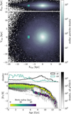 |
Fig. 1 Selection of the stellar particles of the NIHAO-UHD simulation g7.55e11 snapshot 1024 (Buck et al. 2020). Top panel: stellar particles density (number count per pixel) in Galactocentric Cartesian coordinates (in edge-on and top-down views), highlighting the selected solar neighbourhood (1147 stellar particles, highlighted in turquoise). Bottom panel: age distribution and age-metallicity relation of the selected particles, coloured by Galactocentric birth radius. Particles not belonging to the SN selection are shown in grey as reference. |
2.2 From star particles to stellar systems
To translate star particles into individual stars, we created simple stellar populations from a set of stellar evolutionary models. In this work, we used the PARSEC 1.2S + COLIBRI models3 (Bressan et al. 2012; Chen et al. 2015; Marigo et al. 2017; Pastorelli et al. 2020) with standard choices regarding mass loss (ηReimers = 0.2) and YBC bolometric corrections (Chen et al. 2019) with the revised Vega spectrum from Bohlin et al. (2020).
These models use scaled-solar composition with a Z-dependent helium content, microscopic diffusion, nuclear reaction rates from the JINA REACLIB database (Cyburt et al. 2010), the FREEEOS4 equation of state, OPAL opacities (Iglesias & Rogers 1996) except in the low-temperature regime, and a mixing-length parameter (Böhm-Vitense 1958) of αmlt = 1.74.
In practice, for each particle we selected the closest metal-licity and age in a PARSEC grid of evolutionary models, and then sampled a total number of stars (at any evolutionary stage) corresponding to the particle’s mass in the cosmological simulation from an initial mass function. These synthetic single stars were then arranged in stellar systems according to the observed multiplicity statistics (see Appendix A.1).
The stars simulated in this work were generated following the initial mass function (IMF) determined by Kirkpatrick et al. (2024) using a 10 pc volume-complete sample of stars in the solar vicinity. After creating all the stars in the stellar particles, we made a cut in mass, from 0.1 to 1.6 M⊙ in order to keep only stars of type F, G, K and M. O, B, and A stars were excluded because of their short lifetimes and the difficulty in detecting and characterising exoplanets in these systems.
Binary stars are often overlooked as planetary hosts in similar studies (e.g. Madau 2023; Boettner et al. 2024a), as they are systems with complex processes that exhibit a wide variety of instabilities, frequently impacting the stability of the planetary system. Nearby examples, such as the Proxima Centauri system, as well as numerous recent discoveries via transit-timing variations (e.g. Doyle et al. 2011; Kostov et al. 2013; Anglada-Escudé et al. 2016; Getley et al. 2017; Kostov et al. 2020), radial-velocity searches (e.g. Martin et al. 2019), microlensing (Bennett et al. 2016), and imaging companion searches around known planet hosts (Sigurdsson et al. 2003; Mugrauer et al. 2025), show that planets often reside in multiple systems (for recent reviews see Kostov 2023, Deeg & Doyle 2024), orbiting the whole multiple system (‘P-type’ or circumbinary planets, for binary systems) or one of its components (‘S-type’ planets). However, for the purpose of this paper, we focussed exclusively on single stars, not considering exoplanetary systems involving binaries, triples or higher-order multiple stellar systems, nor stellar remnants (white dwarfs, neutron stars, and black holes), due to poor constraints in the present-day exoplanet census. We still included binary and higher-order systems in our stellar population synthesis to obtain a realistic stellar population (see Appendix A.1.) This assumption may lead to an underestimation of the number of exoplanets, as recent studies estimate that around 20% of detected planets orbit multiple systems (see Thebault & Bonanni 2025 for an extensive analysis of the planet-hosting multiple systems). We will include S-type exoplanets in future work.
2.3 Simulating exoplanets
To simulate the exoplanet population orbiting around the simulated stellar systems, we used occurrence rates of different planetary types derived from the literature. We assigned to each single star, depending on its mass and metallicity, a number of Earth-like planets, super-Earth (SE) or Neptunian planets, and sub-giants or giants (see Sect. 2.3.1). Then we assigned a mass and a period to each planet, drawn from bivariate Gaussian distributions obtained by combining observations and planetary formation models (see Sect. 2.3.2). The orbital eccentricity was considered to be zero for all planets, as a first approximation.
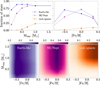 |
Fig. 4 Fractions of single stars harbouring at least one planet of different planetary types. The top left panel shows the occurrence rate as a function of the stellar mass, adapted from Burn et al. (2021). The top right panel shows the occurrence rates as a function of the stellar metal-licity, adapted from Narang et al. (2018). The bottom row shows the joint occurrence rates obtained for each category of planet, combining the stellar mass and metallicity dependencies. |
2.3.1 Occurrence rates and multiplicity
Similarly to stellar multiplicity, the occurrence rates and multiplicities of different planetary types depend on the stellar properties (see, e.g. Sect. 2 of Drążkowska et al. 2023 for a review). In this work, we considered only the dependence on stellar mass and metallicity because these are the most established dependencies. However, there are also indications for additional dependence of planet statistics and composition on stellar age (e.g. Weeks et al. 2025) and detailed chemical composition (e.g. Adibekyan et al. 2012; Tautvaišienė et al. 2022; Cabral et al. 2023; Sharma et al. 2024; Yun et al. 2024). The occurrence rates as a function of stellar mass and metallicity used in this paper (see below) for the three categories (Earth-likes, super-Earths or Neptunes, sub-giants or giants) are presented in Fig. 2, as well as the global occurrence rate obtained by combining those two dependencies.
For the mass dependence, we adapted results from Burn et al. (2021): from a planet formation model (based on the Generation III Bern model; detailed in Emsenhuber et al. 2021a) they derive the fraction of stars harbouring at least one planet of five different types (Earth-like, super-Earth, Neptunians, sub-giants, and giants; see their section 3.2), as a function of the stellar mass. We grouped together the super-Earth and Neptunian planets, as well as the sub-giants and giants, to end up with three categories. As Burn et al. (2021)'s simulations are only available for stars with masses up to 1 M⊙ we use constant extrapolation to extend to our maximum mass of 1.6 M⊙.
There is ample evidence from observations as well as simulations for a dependence of planet occurrence rates on metallicity (e.g. Gonzalez 1997; Fischer & Valenti 2005; Mordasini et al. 2012; Narang et al. 2018). In general terms, there is a consensus that the occurrence rate of giant planets strongly depends on metallicity, while the occurrence rate of rocky planets does not significantly vary with metallicity above a certain metallic-ity floor. There is, however, no consensus on the value of this metallicity floor (e.g. Andama et al. 2024).
In this work, we used the results derived by Narang et al. (2018) from Kepler DR25 results to describe the metallicity dependence of the planet occurrence rate (Fig. 2, upper right panel). To match our three planet categories, we combined their data for the 2-4 R® and 4-8 R® planets in one group, corresponding to our super-Earths & Neptunes category. We conservatively set the occurrence rate to zero for metallicity lower than −1.0 and higher than 0.6, reproducing the lower and upper limits of the detected host-star metallicity distribution.
To combine the dependencies of the planet occurrence rate on the stellar mass and metallicity, we assumed that they are independent. We multiplied the occurrence rate as a function of stellar mass with the occurrence rate as a function of [Fe/H], normalised such that we match the occurrence rate of Burn et al. (2021) for stars with [Fe/H] = 0 (see Fig. 2). When we obtained a combined occurrence rate greater than 1, we considered it equal to 1.
For our single stars sample, we drew their probability of harbouring at least one planet of each planet type using the combined occurrence rate. Then we drew the number of planets of each type using the multiplicity as a function of the stellar mass given by Burn et al. (2021), combining again their 5 categories in 3 by simple addition. The number of planets of each category is drawn randomly following a Poisson distribution centred on the multiplicity value at their stellar mass.
2.3.2 Mass-period distributions
We then assigned fundamental astrophysical parameters to all created planets, in particular mass and orbital period. The distribution of confirmed exoplanets from the NASA Exoplanet Archive (Akeson et al. 2013; Christiansen et al. 2025) shows clear observational biases, with an over-representation of hot Jupiters and a lack of Earth-like planets, due to the large detectability dependence on planetary radius and orbital period (Sect. 4.2). We aim to account for this bias by combining the observed distribution with predictions from a planetary formation model. We approximated the Mass-Period distribution of the different planet categories by bivariate Gaussians. For the super-Earth & Neptunian planets and the giants, the bivariate Gaussians parameters were chosen to reproduce the observational data (confirmed exoplanets from the NASA Exoplanet Archive). For the Earth-like population, we adjusted the bivariate Gaussian parameters such that they reproduce the combination of the distributions shown in Drążkowska et al. (2023, both panels of their Fig. 13)5. The four bivariate Gaussian distributions are overplotted as light grey contours in Fig. 3, and their parameters can be found in Table A.1.
We assigned a random mass and orbital period to all planets, sampling from the bivariate Gaussian associated with their assigned type. For the sub-giants & giants category, we randomly distributed them between hot Jupiters (‘HJ’) and cold or warm Jupiters (‘CJ’), with a 10% probability of being a HJ. We redrew the parameters for planets with masses greater than 104 M® (the lower mass limit of brown dwarfs; e.g. Burrows & Liebert 1993; Joergens 2014) as well as planets with a distance to their host star lower than two times the stellar radius.
In what follows, we use these assigned planet masses to classify the exoplanets into the different planetary types (see the boundaries used in Table 1), instead of the original parent Gaussian in Fig. 3, which could be incompatible with the drawn mass value. A priori, we can think of several different ways to classify exoplanets into planet types, for example by mass, by radius, or by density. In Fig. 4 we compare the percentages obtained for the volume-complete SN (see Sect. 3) using three different classifications: 1. ‘labels’, using the planet type first assigned using the combined occurrence rate of the different planet types (see Sect. 2.3.1 and Fig. 3); 2. ‘mass’ ; and 3. ‘radius’ using the boundaries set in Table 1. As we assigned masses drawing from broad bivariate Gaussian distributions, the associated mass can end up being incoherent with the initial label, leading to differences in the percentages of each planet type. To achieve consistent classifications, we used mass-based categories for the simulated exoplanets and radius-based definitions for the Kepler exoplanets (since Kepler exoplanets are detected by transit, they have accurate radius measurements instead of mass). It would be ideal to use the same category definition for simulated and observed planets, but there are not enough accurate mass measurements for planets detected by Kepler. Thus, our conversion from masses to radii for simulated planets adds another important uncertainty.
In addition, we did not correct for potential overlaps of orbits within a planetary system, nor did we consider the systems’ dynamic stability. In Fig. A.1, we show the architecture (planet distribution vs. semi-major axis) of 40 randomly selected synthetic planetary systems, sorted by stellar mass. We insist that we do not currently aim to produce realistic planetary architectures (see, e.g. Howe et al. 2025), but only try to reproduce the overall statistics of the observed exoplanet population (see Sect. 4 for a comparison with the Kepler field). Dedicated analyses of the variety of exoplanet architectures found by Kepler (e.g. Fabrycky et al. 2014; Lissauer et al. 2024), CHEOPS, and TESS indeed reveal signs of orbital resonances (Luque et al. 2023; Dai et al. 2024), instabilities (Ghosh & Chatterjee 2024), dynamical packing (Obertas et al. 2023), etc. that are out of the scope of this work. The exoplanetary population obtained in this work is only expected to show realistic properties in terms of metallic-ity, effective temperatures, radius of the planets, and semi-major axis of their orbits. Mishra et al. (2021) suggested to divide the planetary systems’ architecture into 4 classes: similar, antiordered, ordered, and mixed. Without imposing any constraint on the system’s architecture (not correcting orbits overlaps, not considering resonances), we obtain similar frequencies to the Bern model used by Mishra et al. (2021): see lower panel of Fig. A.1.
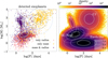 |
Fig. 3 Distribution of detected vs. simulated exoplanets. Left panel: detected exoplanets from the NASA Exoplanet Archive. Planets with both mass and radius measurements are shown in purple, and the ones with only mass measurements are in yellow. Planets with only radius measurement are in red (using the radius-to-mass conversions of Parc et al. 2024), but were not used to derive the bivariate Gaussian distributions. Right panel: density distribution (number count per pixel) of the 24.5 million simulated exoplanets in the solar vicinity. In grey lines are overplotted the bivariate Gaussian distributions used to assign a mass and a period to each planet randomly. The distribution of giants (HJ and CJ) and SE & Neptunes were chosen to reproduce the confirmed exoplanet population (see left panel) while the Earth-like distribution was based on the distribution predicted by (Drążkowska et al. 2023, their Fig. 13). |
Planet types definitions, based on Burn et al. (2021) for masses and on Narang et al. (2018) for radii.
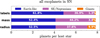 |
Fig. 4 All simulated exoplanets in the volume-complete SN. Influence of the planet type definition on the obtained occurrence rate, comparing three different definitions for the exoplanet categories: using the original labels, the mass or the radius. |
3 Results for the volume-complete solar neighbourhood
In this section, we describe our results obtained for a volumecomplete solar neighbourhood (of approximatively 1 pc3) in our fiducial galactic simulation. We compare the simulated exoplanets to observed exoplanets in Sect. 4.
3.1 Simulated stellar population
As described in Sect. 2.1, we started by selecting the 1147 stellar particles corresponding to the SN in the galaxy g7.55e11's redshift-zero snapshot (Fig. 1). From the stellar particles, we created 9.1 million individual stars, from which we kept only FGKM stars (Sect. 2), excluding stars with mass greater than 1.6 M0: we obtain a total sample of around 8.3 million stars. After the creation of stellar systems as detailed in Appendix A.1, we obtain around 3.4 million single stars, 3.6 million in binary systems, and 1.3 million in higher-order systems. The total stellar density in our SN selection is around 0.005 M⊙ ∙ pc−3, while the latest estimation based on observations gives results around 0.04 M⊙ ∙ pc−3 (Lutsenko et al. 2025). The Hertzsprung-Russell diagram and the distribution in mass-metallicity diagram are shown in Fig. 5.
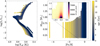 |
Fig. 5 All simulated stars in the volume-complete SN of the g7.55e11 galactic simulation. Left panel shows the Hertzsprung-Russell diagram, colour coded by age. Right panel shows the distribution of stellar mass versus metallicity, also colour coded by age. The zoom-in panel shows the density distribution of stars in the region of the mass-metallicity space plotted in Fig. 2. |
3.2 Exoplanet demographics in the simulated solar vicinity
Simulating exoplanets only around single stars as described in Sect. 2.3, we end up with a total sample of 22.6 million planets, organised in 2.9 million planetary systems and composed of around 52.5% of Earth-like planets, 44% of super-Earths and Neptunians, and around 3.5% of giants and sub-giants. About 23% of them are located in the circumstellar habitable zone (CHZ; see Sect. 3.4). The distribution of the exoplanet sample in the mass-period diagram is shown in Fig. 3. We stress that, by construction (see Table A.1), our mass-period diagram reproduces the observed data for cold and hot Jupiters, as well as super-Earths and Neptunes (as reported in Fig. 13 of Drążkowska et al. 2023).
Fig. 6 shows the effective temperature vs. instellation (the intensity of the received star’s radiation, in surface power density) diagrams for our simulated solar vicinity sample, compared to all currently confirmed exoplanets in the NASA exoplanet database. The left panel of Fig. 6 contains the full sample of planets, while the other panels correspond to our sub-categories Earth-like, super-Earths & Neptunes, and giant planets. Overall, our distribution is compatible with the observed exoplanet populations, with the exception of the giant planets, whose observed distribution covers a wider parameter space than our simulation. The major difference we observe for cool stars is due to a strong observational bias: the majority of our simulated exoplanets orbit M-type stars, the most abundant stellar type (Reylé et al. 2021 estimate that they represent around 60% of all stars within 10 pc), which are underrepresented in the actual detections because they are so faint (for reference, they represent less than 2% of the stars observed by Kepler).
3.3 Representativeness of exoplanet host stars of the underlying population
Comparing the properties of planet-hosting stars to those of the general stellar population is a common technique employed in observational exoplanet studies (e.g. Adibekyan et al. 2012; Bashi et al. 2020; Tautvaišienė et al. 2022). Indeed, these studies are necessary to calibrate the dependencies of the occurrence rate and multiplicity (see Sect. 2.3.1). Here, we compare the effect of our occurrence rate prescriptions on stellar parameters that do not directly influence the occurrence rates, such as age and birth radius (although both of these parameters are indirectly linked to metallicity through Galactic chemical evolution; see, e.g. Chiappini et al. 2001; Minchev et al. 2018).
Our model predicts that only 14% of the single stars in the solar vicinity do not host exoplanets. In Fig. 7 we compare the distribution in age, stellar mass, birth radius, and metallicity [Fe/H] of the entire population (‘all stars’, in grey) with that of the single stars with planets (in blue) and single stars without planets (in red). Since the fraction of planet-hosting stars is large, we find only subtle differences between the planet-hosting and the entire stellar population. On the other hand, we do observe pronounced differences between non-hosting single stars and planet hosts. The most important difference is that around half of the non-hosting stellar population are metal-poor stars (and thus mostly old), while almost all hosting stars have a metal-licity greater than −0.5. This is partly due to our modelling of the planet occurrence rate, set to 0 for stars with [Fe/H] ≤ −1.0; see Fig. 2 and Sect. 2.3.1. We also note that the non-hosting stars group contains a non-negligible fraction of accreted stars that were born outside of the main galaxy (see birth radius distribution on the lower left panel of Fig. 7).
3.4 Planets in the circumstellar habitable zone
The circumstellar habitable zone (CHZ) is the region around a star in which liquid water might exist on the surface of orbiting planets. This zone is considered a key factor in determining the potential for life as we know it, since liquid water is essential for life on Earth. For this reason, one of the primary objectives of the Kepler mission was to determine the occurrence rate of rocky exoplanets in the CHZ of solar-like stars (Borucki et al. 2010; Borucki 2016), often referred to as η⊕. Many studies have since derived estimates of η⊕, with values ranging from <1% to >50% (see, e.g. Appendix 2 of Scherf et al. 2024). The boundaries of the CHZ depend mainly on stellar luminosity and effective temperature, although other factors are sometimes included (e.g. Kaltenegger 2017; Lammer et al. 2024). The optimistic HZ is delimited empirically by the ‘recent Venus’ and ‘early Mars’ limits, i.e. set by the last time liquid surface water could have existed, respectively on Venus and Mars (S/S⊕ = 1.78 and S/S⊕ = 0.32 for Teff = 5800 K; Kasting 1988; Kaltenegger 2017). Here, we use this optimistic definition of the CHZ (see Fig. 6).
In order to assess whether our simulated planets are in the CHZ of their host stars, we used the polynomial equations from Kopparapu et al. (2013) to determine the limits of the CHZ. We find that ~23% of our solar-vicinity exoplanets lie in the CHZ of their host star (~25% of the Earth-likes, ~20% of the superEarths and Neptunes, and ~29% of the giants), a result which is higher than most of the literature values cited above. This can be explained by the extreme under-representation of Earth-like planets in observations compared to the underlying population, as visible in Fig. 6.
4 Forward-modelling the Kepler exoplanet census
The significance of the Kepler mission Borucki et al. (2010) for exoplanetary science can hardly be overestimated (Lissauer et al. 2023). The Kepler field in the constellation of Cygnus, with its more than 4000 exoplanet candidates (Lissauer et al. 2024), is thus the natural testbench for exoplanet population models. In this section, we provide forward simulations of the exoplanetary population in the Kepler field based on the method described in Sects. 2 and 3, taking into account the most important selection effects of the original Kepler mission. This allows us to evaluate the overall quality of our exoplanet simulation and helps us identify ways for future improvements.
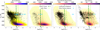 |
Fig. 6 Effective temperature of the host stars vs. instellation at the simulated exoplanet for the volume-complete SN sample. For comparison, we overplot the distribution of the observed exoplanets (Christiansen et al. 2025) as black dots and the solar-system planets as cyan diamonds. The left panel shows the entire sample, while the other three panels show the distribution of each planet category (Earth-like, SE and Neptunians, giant planets). The limits we adopted for the definition of the CHZ are plotted in dark and light green (see Sect. 3.4). |
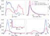 |
Fig. 7 Stellar age, mass, birth radius, and metallicity density distributions for the SN simulation. In each panel, we show the distributions of all simulated stars, stars without planets, and stars with planets, as indicated in the legend (single stars without planets represent ∼14% of the single star population). |
4.1 Kepler selection function
To produce a simple mock sample of the Kepler field, we used the same galaxy g7.55e11 presented in Sect. 2.1. We now focus on a sky area that matches the Kepler field in size and position (see Fig. 8 top left panel). Stars and planets were created following the methods described in Sect. 2, with an additional dispersion in the galactic coordinates to ensure a smooth sampling: we first selected all stellar particles in a wide cone around the Kepler field of view up to a distance of 5.5 kpc from the Sun, to include all Kepler exoplanets. Then, we generated the stellar population following the methods described in Sect. 2.2, before sampling the galactic coordinates of all created stars, following a Gaussian distribution centred on the coordinates of their host stellar particle, with a dispersion of 500 pc in XGal and YGal and of 100 pc in ZGal. Finally, we selected the stars located in the Kepler field, using K2fov package (Mullally et al. 2016). Interstellar extinction, although low in most of the Kepler field (Rodrigues et al. 2014), was added using the 3D extinction map of Green et al. (2019) included in the dustmaps package (Green 2018). Finally, we converted the obtained reddening E(B - V) to extinction in the Gaia G band using AG ≃ 0.84 ∙ AV, and AV = 3.1 ∙ E(B - V). The top left panel of Fig. 8 shows the resulting extinction distribution.
To obtain a stellar population comparable to the Kepler target list (Batalha et al. 2010), we applied the selection fraction as a function of magnitude derived by Wolniewicz et al. (2021) (their Fig. 2b) to the full sample of generated stars. Additionally, we discarded all stars with apparent magnitude G > 16, as well as giants (defined as log(g) ≤ 4) with magnitudes G > 14, to match the actual observed fraction (their Fig. 2a).
After those two magnitude cuts, our sample contains ~31000 stars, with an overrepresentation of stars with magnitudes between G = 15.5 and G = 16. The target selection of Kepler is based on criteria we did not consider, such as the minimal planetary radius expected to be detectable, Rp,min (Batalha et al. 2010). As we are not able to compute this quantity for our simulated population, we modified the magnitude selection function taken from Wolniewicz et al. (2021) to match the final magnitude distribution of Kepler target stars (Wolniewicz et al. 2021; Farmer et al. 2013) (top right panel of Fig. 8). We end up with around 20 000 ‘observed’ stars in the Kepler field, this number being ~12% of the stars actually observed by Kepler6. One of the factors explaining this difference is that we consider only the single stars from our simulation, while some observed stars in the Kepler field are unresolved binaries. However, including all the primary stars (making the same magnitude cuts) would not even double our observed star population. The difference in star counts is thus mainly due to the lower stellar density in the simulation compared with the actual SN (see the first paragraph of Sect. 3).
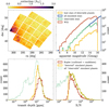 |
Fig. 8 Summary of our simulation of the exoplanet population in the Kepler field. Upper left panel: geometric selection of stars in the simulated Kepler field, colour-coded by interstellar extinction in the G band, AG. Upper right: apparent G magnitude distribution of all simulated stars in the field of view (in blue), the ‘observable’ stars, as selected in Sect. 4.1 (green), compared to the stars observed by Kepler (Wolniewicz et al. 2021 catalogue, in red). Lower panels: transit depth and transit signal-to-noise distributions of planets in the Kepler field. Red: observed distribution among candidate+confirmed Kepler exoplanets. Green: all simulated planets with orbit inclinations compatible with a transit observation (see Sect. 4.2). Yellow: simulated detected exoplanets (i.e. planets with S/N ≥ 7.1). |
4.2 Selection of observable transiting exoplanets
We applied our exoplanet generation process to the simulated stars which would be ‘observed’ by Kepler (around 20 000, see Sect. 4.1), and obtain around 170000 exoplanets. Assuming a random inclination (see Appendix B.3) and ephemeris distribution of the planets orbiting each star, we calculated the detection probability of each exoplanet during a Kepler-like single-star observation campaign of 4 years. In order to simulate the observability of synthetic exoplanets by Kepler, we first estimated the signal-to-noise ratio (S/N) of each exoplanet transit. In practice, we used equation (4) of Christiansen et al. (2012):
 (1)
(1)
In this equation, the number of observed transits Ntr is obtained from the planet’s orbital period P, the total observational time of Kepler tobs, and the fraction of this total time when the target was observed, f, = 0.92, following Christiansen et al. (2012). The transit depth δ = (Rpl/Rst)2 is the squared ratio of the planet’s and host star’s radius (shown in the lower left panel of Fig. 8). Planet radii Rpl were estimated from the planet masses, see Appendix B.2 for details. The secondary peak around 1 ppm in the transit-depth distribution is due to the (mostly undetectable) Earth-like population. Finally, the CDPPeff is the effective combined differential photometric precision, a photometric precision metric. It was experimentally measured during the Kepler mission (Koch et al. 2010; Jenkins et al. 2010); we give more details on how we estimated it for our synthetic planets in Appendix B.3.
We consider a planet to be synthetically ‘detected’ by Kepler if its S/N ≥ 7.1: our fiducial ‘detected’ sample for the Kepler field of view contains around 6200 planets, orbiting 2400 host stars7. The final S/N distribution is shown in the bottom right panel of Fig. 8.
To test our synthetic S/N estimates on real data, we applied them to all candidates and confirmed planets from Kepler. The results are shown in Fig. B.2: the one-to-one comparisons with Kepler demonstrate that 1. the transit depth is retrieved with very good accuracy and precision, and 2. our S/N estimates are globally accurate, albeit with a slightly higher dispersion compared to the published values by Kepler (koi_model_snr), see Appendix B.4.
4.3 Comparison of simulated ‘detectable’ exoplanets with Kepler planets and candidates
We now proceed to a more detailed comparison of the Kepler exoplanet census with our tailored simulation described in the previous subsections. This allows us to identify potential problems with our simulations and to propose ways to overcome them in the future.
In the lower panels of Fig. 8, we compare the transit depth and S/N distributions of our simulated ‘detected’ exoplanet sample with the Kepler exoplanet catalogue. We obtain similar distributions, with an overdensity of planets with transit depths between 10 and 300 compared to the Kepler data. The total number of ‘detected’ planets (around 6200 planets around 2400 host stars) is similar to the observed population (Kepler DR25: 4619 around 3024 host stars), despite having ~10 times fewer simulated stars than observed ones. We notice that we tend to observe too many exoplanets per star (see Sect. 4.3.2). This is likely a consequence of the fact that 1. we do not model stellar variability which further degrades the CDPP, 2. we assume that all planets of a system are perfectly aligned in the same orbital plane, and 3. we estimate each exoplanet’s detectability individually, even in multi-planetary systems (a minor effect for transit surveys like Kepler).
4.3.1 Comparison of host star properties
Starting with the Kepler Input Catalogue (Brown et al. 2011), several works have presented stellar parameters for stars (and in particular planet hosts) in the Kepler field (e.g. Huber et al. 2014; Johnson et al. 2017; Berger et al. 2020; Zhang et al. 2025). For our comparison, we used the homogeneous stellar parameters obtained from Gaia DR3 low-resolution XP spectra and parallaxes combined with broad-band photometry by Khalatyan et al. (2024).
In Appendix B.1, we compare the distributions of apparent magnitudes, distances, effective temperatures, and stellar radii of our synthetic ‘detected’ host stars with the ones from the Kepler catalogue (candidates + confirmed exoplanet hosts). The key differences are: (1) our simulation predicts a larger population of F-type main-sequence planet hosts than observed, and (2) our simulation also predicts more giant-star planet hosts than observed by Kepler (see bottom panels of Fig. B.1). These discrepancies arise because the g7.55e11 simulation differs from the Milky Way disc in some important parameters. Among them, one notable difference is the over-representation of young stars, caused by a rather late peak in the star-formation history, and leading to an over-representation of hot stars (Teff > 6000 K, see middle left panel of Fig. B.1). The distance distribution discrepancy (top right panel) can be explained by the larger vertical velocity dispersion and scale height of the disc in g7.55e11 compared to the MW (see also Sect. 7.1).
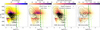 |
Fig. 9 Effective temperature vs. instellation, analogous to Fig. 6, but for the simulated Kepler field. The distribution of the exoplanets observed by Kepler is shown as black dots, while the distribution of ‘detectable’ exoplanets in the Kepler simulation is shown in black density contours. The background distribution shows the distribution of planets after applying magnitude cuts described in Sect. 4.1. The number of detectable exoplanets in the simulated Kepler field is indicated on the lower left part of each panel. |
4.3.2 Comparison of planet occurrence rates
As discussed in Sect. 4.2, although the number of our simulated ‘detectable’ exoplanets in the Kepler field is comparable to the confirmed+candidate exoplanets detected by Kepler (several thousands), we find too many planets per star, with a mean of 2.56 ± 0.04 planets per host star, versus ~1.3 for Kepler. In Fig. 9, we show a comparison of the observed and simulated exoplanet families in the Teff vs. instellation plane (analogous to Fig. 6). We see that our simulation overpredicts the number of SE & Neptunes, while it underpredicts the number of Earthlike planets: we obtain 5% of Earth-like planets, 85% of SE & Neptunes, and 10% of giants, while Kepler confirmed exoplanets are composed of 14% of Earth-like, 74% of SE & Neptunes and 12% of giants.
The percentage obtained for each planet type depends on the definition we adopt. While the percentage of Earth-like planets is stable throughout the different definitions we compared, the percentage of SE & Neptunes and sub-giants & giants varies more strongly. As discussed in Sect. 2.3.2, we chose to use the massbased definition for our simulated exoplanets in Sects. 3, 5, and 6. For our comparison with the Kepler planets in this section, however, we chose to use the radius-based definition, since very few of the Kepler planets have mass estimates.
4.3.3 Comparison of planet masses and radii distributions
Fig. 10 shows the mass-period and the period-radius diagrams of our forward-simulated ‘detected’ exoplanets, compared with the observed Kepler population. The mass-period diagram follows, by construction, the populations shown in Fig. 3, modulo the (heavy) selection effects simulated in Sects. 4.1 and 4.2. Since precise masses are not readily available for most of the observed Kepler exoplanets, we only show the observed population in the period-radius diagram (lower panels of Fig. 10).
After simulating detectability, we have fewer planets with small radii than the actual confirmed cases by Kepler. We suggest that this discrepancy is caused by (1) planets that were confirmed by follow-up observations, and (2) our mass-to-radius conversion (see Appendix B.2), which might be too simplistic. Another well-known feature of the Kepler data that we do not reproduce is the so-called ‘radius gap’, a bimodality in the radius distribution of small planets (e.g. Fulton et al. 2017; Zeng et al. 2017; Petigura et al. 2022), which is expected since we did not explicitly include it in our modelling (see caveats in Sect. 7.1).
Another subtle effect that is seen in the data but not in our model is the photo-evaporation of close-in planets (with periods ≲3 days): planets that initially lay between the low-density sub-Neptunes and the dense super-Earths are likely to lose their atmospheres by the intense radiation of the nearby host star, which results in a gradual decrease of the planet radius over time (see McDonald et al. 2019 for a summary). They end up in lower regions of the R - P space. This phenomenon is complex, depending on the planet’s and atmosphere’s composition, as well as on the stellar type of its host star. We therefore confirm that neither the radius gap nor the missing close-in Neptunes (generally attributed to photo-evaporation) are caused by selection effects. In the future, we aim to introduce some of these more intricate properties of the exoplanet population into our modelling.
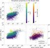 |
Fig. 10 Comparison with exoplanets in the Kepler field (mass-period and radius-period diagrams). The left column shows the exoplanet population obtained by our simulation. The right plot shows the exoplanets found by Kepler (both candidates and confirmed). Top panel: planet mass (in M⊕) vs. orbital period (in days). Bottom row: planet radius (in R⊕) vs. period. For the simulated exoplanets, the radius was obtained with a conversion from the planet mass (see Appendix B). |
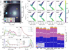 |
Fig. 11 Results of our planetary population synthesis for different regions in the MW-like galaxy g7.55e11. Top left panels: Illustration of the regions studied, in Galactocentric Cartesian co-ordinates. Top right panels: metallicity-coloured Hertzsprung-Russell diagrams for each of the regions. Bottom left panels: Stellar age (A), stellar mass (B), birth radius (C), and metallicity (D) distributions, analogous to Fig. 7. Bottom right panel: Relative planet occurrence statistics for each of the studied regions. |
5 Exoplanet populations in different regions of the simulated galaxy
The impact of the galactic environment on planet formation and evolution has been debated since the seminal paper of Gonzalez et al. (2001) who coined the term Galactic Habitable Zone (see also e.g. Lineweaver et al. 2004; Prantzos 2008; Gowanlock et al. 2011; Baba et al. 2024). In this and the following section, we refrain from discussing this concept in detail, but study the distribution of different types of exoplanets as a function of galactic environment, using the same simulation framework used to study the solar vicinity (Sect. 3) and the Kepler field (Sect. 4). Bashi & Zucker (2022) opened the studies about the influence of the Galactic context on the exoplanet formation, with a sample of 506 planet candidates from Kepler DR25 orbiting 369 host stars, associated to either the thin disc (292 stars), the thick disc (7 stars) or the halo (0 star). They find that thin disc stars (mostly young and metal-rich) host on average more planets than thick disc stars (mostly old and metal-poor). Their sample being limited by its size, it is interesting to use Galactic simulations to study the exoplanet distribution in the Galaxy.
In this section, we study the simulated exoplanet populations in eight regions of the galaxy g7.55e11 (summarised in Fig. 11). In addition to the solar vicinity sample studied in Sect. 3, we selected seven regions that cover the full extent of the galaxy’s disc and bulge, each containing a similar number (~1000) of stellar particles. The top left panel of Fig. 11 shows the location of the seven additional regions: i) an outer-disc region (RGal ~ 15 kpc; cyan), ii) an inner-disc region (RGal~4 kpc; green), iii) the galactic centre (dark violet), iv) two regions similar to the SN selection but at different angles (φGal = 60°, 300°, respectively; yellowish colours); v) two regions with the same distance to the galactic centre than the SN, but situated above and below (2.5 kpc < |ZGal| < 4 kpc) the galactic disc, respectively (pink colours).
In the top right plots of Fig. 11, we show the Hertzsprung-Russell diagrams of the simulated stars in each of the eight regions highlighted in the top left panel of that figure, reflecting the impact of the different age and metallicity distributions on the stellar population in each region. The bottom row of Fig. 11 shows the distribution of the simulated stellar population in age, mass, birth radius, and metallicity (lower left panels) and the relative planet occurrence statistics (lower right panels) for each of the eight selected regions.
We first analyse the stellar populations of the eight regions. We observe very little variation in the stellar mass distribution - this is expected because we assume the IMF to be invariant. Regarding the metallicity distributions within the different regions, we find a clear signature of the negative radial metallicity gradient: the galactic centre region is predominantly metal-rich, and the peak [Fe/H] moves to gradually lower values for the inner region, the SN, phi60, phi300, the upper and lower, and finally the outer region. The upper and lower regions both contain a significant metal-poor tail, as expected, corresponding to potential accreted/halo stars. Studying the host star population in those metal-poor regions is interesting to verify whether such objects can be observationally found and to further explore those regions in search of potential accreted exo-planetary systems, as proposed by Perottoni et al. (2021). The centre region has a secondary peak around [Fe/H] ≃ −0.4, reflecting the complex stellar population mixture that we also observe in the centre of the Milky Way (e.g. Schultheis et al. 2015, 2020; Nieuwmunster et al. 2023; Nandakumar et al. 2024).
The birth radius distributions of all regions are approximately Gaussian, centred on the central radius of the respective region. The dispersion in birth radius increases with distance from the galactic centre (and distance from the disc plane, for the high-|Z| regions). This is mostly due to an increase in the fraction of accreted stars towards the outer disc, while radial migration within the disc dominates in the inner and SN regions. Finally, the age distributions in Fig. 11 reflect the significant differences among the star-formation histories of the eight regions of g7.55e11. As expected, the two high-|Z| regions do not contain any young stars (<4 Gyr). The age distributions reflect the inside-out formation of the galaxy, with the peak of the age distribution shifting towards lower ages as we move from the inner to the outer galaxy. Consistent with its metallicity distribution, the age distribution of the galactic-centre sample is also very broad.
Regarding the exoplanet populations in the eight regions of g7.55e11, we find that the number of planets per star is similar between all regions (between 6 and 7), except for the upper and lower regions which present a mean number of 4 planets per star (due to the lower mean metallicity of the stars found in those regions). The planet type fraction is similar in all of them (52-58% Earth-like, 39-44% SE & Neptunes, 2.6-3.5% giant planets), with slight variations caused by the stellar-population differences. For example, the outer region displays a relative fraction of Earth-like planets that is ~5% higher than in other regions, and the lowest percentage of giant planets (see Sect. 7 for a discussion).
Recently, Boettner et al. (2024a) also investigated variations in galactic planet populations using a different methodology. They combined a high-resolution Milky Way analogue (“37_11 run”) from the HESTIA suite of simulations (Libeskind et al. 2020) with the Bern planet formation model (the New Generation Planet Population Synthesis, NGPPS; Emsenhuber et al. 2021b). The stellar particles of this galactic snapshot have a typical mass of ~104 M⊙. They created the stellar population from all the stellar particles, assuming uniform age and metallicity, and sampling masses from the Chabrier (2003) IMF around a unique value M* = 1 M⊙ ± 5%, keeping only the main sequence stars, to obtain a total number of stars N*. For each stellar particle, they assigned a certain number n of planets of different categories per host star, obtained from the NGPPS model (assuming the initial number of embryos Nembryos = 50 and the stellar mass M* = 1 M⊙). They finally obtain the total number of planets: Npl = n × N*. Applying this framework, they compare the obtained occurrence rates in metal-rich regions (bulge, thin disc) with metal-poor regions (thick disc, halo). Discrepant from our findings (in which the relative proportions among different planet types remain fairly constant throughout the Galaxy; see Fig. 11), they find that giant planets (>300 M⊕) are 10-20 times more frequent in the thin disc, while Earth-like planets are 1.5 times more abundant in the thick disc. Low-mass planets are widespread across all regions. Comparing yields using uniformmass population of lower stellar mass (0.3-0.5 M⊙), they find that the trends are weaker for low-mass dwarfs than solar-mass stars, leading to more homogeneous results across the galaxy. As they base their galactic analysis only on 1 M⊙ stars, while we consider a broader range of stellar masses, we expect to obtain weaker occurrence variation between galactic environment.
6 Comparison of the same region in different simulated galaxies
In this section, we investigate the impact of the simulated galaxy choice on our results. It is well known that the morphology and physical properties of disc galaxies vary considerably (Dutton et al. 2010, 2017, e.g.). Even when ‘Milky-Way-like’ galaxies are explicitly selected from large simulation suites (e.g. by mass, rotation curve, bar, and spiral features), we often find striking differences between the individual galaxies (e.g. Grand et al. 2024; Pillepich et al. 2024). We therefore investigate how the details in the evolutionary history of a galaxy impact the resulting exoplanet population in a solar neighbourhood-like volume, using the other five publicly available final snapshots from the NIHAO-UHD simulation suite of Buck et al. (2020).
In order to compare the solar-neighbourhood-like populations of different galaxies, we used the same spatial definition used in Sect. 2.1 for all final snapshots (see Fig. 12, top panel)8. The differences between the six simulated galaxies are extensively discussed in Buck et al. (2020); we summarise their main characteristics in Table 2. All except g1.12e12, which has a lenticular shape, are clearly disc galaxies with spiral features. The most massive system, g2.79e12, also exhibits a prominent bar.
The lower part of Fig. 12 shows the distribution of the simulated stellar population in age, mass, birth radius, and metallicity (lower-left panels) and the relative planet occurrence statistics (lower-right panel) for each of the simulated solar neighbourhoods in the NIHAO-UHD simulation suite.
Fig. 12 demonstrates that the exoplanet population of a simulated solar neighbourhood does not depend drastically on the particular galaxy and its past history (reflected by the age, birth radius, and metallicity distributions), as long as it is broadly compatible with the main features of the Milky Way. This is illustrated by the little variations we see in the relative proportions of exoplanet types (lower right panel of Fig. 12). Even though there are important differences in the star-formation histories of the six galaxies, the only galaxies for which the relative occurrence rates of Earth-like vs. gaseous planets differs significantly from our fiducial simulation (g7.55e11 discussed above) are 1.12e12 (the lenticular galaxy, which hosts an important old and metal-poor population) and, to a lesser extent, 6.96e11. This galaxy is smaller than our fiducial galaxy, and the chosen solar vicinity is therefore relatively further outwards from its galactic centre, as well as metal-poorer (and thus compatible with our findings in Sect. 5).
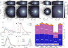 |
Fig. 12 Results of our planetary population synthesis for solar neighbourhood analogues in the six publicly available NIHAO-UHD galaxies, similar to Fig. 11. The top row highlights the selections of the solar vicinity volumes (8.2 kpc from the galactic centre, see Sect. 2.1) in each of the final snapshots. Each selection, except for the more lenticular galaxy 1.12e12, contains between 2 and 4 million stars. The lower panels show the simulated stellar and exoplanet statistics and are analogous to Fig. 11. |
Main properties of the 6 simulated galaxies from NIHAO-UHD suite, compared to the MW.
7 Discussion and conclusions
In this paper, we have studied the exoplanet population from a galactic perspective. We created a framework that generates a synthetic exoplanet population based on a state-of-the-art galaxy simulation that reproduces the most important features of the Milky Way. Focussing first on the Solar Neighbourhood (SN; Sect. 3), we constructed stellar populations and allocated planetary systems to single stars using a prescription informed by both exoplanet statistics and planetary formation models.
For the 3.4 million single stars generated in the SN, we obtain 22.6 million planets. They are distributed in 2.9 million planetary systems, with a mean of 6.7 exoplanets per star (~7.8 per host star). The minority of single stars that do not host any planets are globally older and more metal-poor than the general population (Fig. 7). Using mass-based planet type definitions, 52.5% of the generated planets are classified as Earth-like, 44% as SE & Neptunes, and 3.5% as sub-giants & giants. Among them, 22.5% are located in their host star’s CHZ (24.5% of the Earth-like, 19.8% of the SE & Neptunes, and 29.1% of the sub-giants & giants; Fig. 6). Our models rely on the mass and metallicity dependencies of planet occurrence rates derived from the literature. In this way, we are able to extrapolate exoplanet population properties to different galactic environments. As expected, the majority of exoplanets are located in planetary systems around M stars (see Fig. 6) because these are the most abundant stars, although they are observable only in very close-by systems.
To further validate and test our modelling, we also created a full forward simulation of the Kepler satellite’s census of exoplanets (Sect. 4, Figs. 8-10, Appendix B). Our modelling relies on the same galaxy simulation and includes detailed prescriptions for Kepler’s observing campaign. This experiment results in a comparable number of exoplanets compared to the observed Kepler census, with a similar distribution as Kepler for giants, HJ and CJ (see Fig. 10). However, the Kepler modelling also demonstrates several shortcomings of our modelling that will be addressed in the future (see below).
When extending our modelling to different regions of the same galaxy (Fig. 11), we find that thick disc, halo, and outerdisc regions host less planets per star than the SN and other more central regions of the galaxy9, as well as more Earth-like planets in proportion. The main driver for this is the metal-licity dependence of the planet occurrence rates. Comparing the SN equivalent in different galaxies of the simulation suite (Fig. 12), we again find that the main factor of difference in planet type occurrence rates is the metallicity distribution of the stellar population. More metal-poor galaxies have a smaller number of planets per star, and host fewer giant planets, but (in percentage) more Earth-like.
In total, we obtain ~6.7 planets per star, higher than the Boettner et al. (2024a) estimate (~5.6) or the one of Hsu et al. (2019) (~5.0). As discussed below, our higher estimate could be influenced by some of the approximations used here.
7.1 Caveats and future work
We recall the several limitations in our analysis that should be addressed in future work:
Our sample excludes planets in binary or higher-order star systems, which may influence the overall occurrence rates;
Exoplanet formation yields are strongly metallicity-dependent, yet the precise relationship between occurrence rates and stellar [Fe/H] remains poorly constrained. Improved models incorporating the joint dependence of planet occurrence on stellar mass and metallicity are needed. In particular, we assumed very conservative limits for the occurrence rate below [Fe/H] = −1, which will only be improved by future space missions like PLATO and HAYDN;
The conversion from planetary mass to radius introduces significant uncertainty due to the degeneracy in composition and structure models;
By defining planet types based on mass rather than originally assigned planet types, we inherently modify the original occurrence rates. In the future, we will improve this categorisation by combining masses and radii to define the planetary types by density. This will allow us to obtain a finer division between Earth-like planets, super-Earths, water worlds, sub-Neptunes, Neptunes, etc.
Our model does not account for orbital resonances or system architecture, which may affect the detectability and distribution of planets;
We do not incorporate the observed radius gap nor the Neptune desert, which requires a clearer distinction between super-Earths and sub-Neptunes in future work. We plan to incorporate different photo-evaporation effects in a future version of our exoplanet simulation.
Our full forward simulation of the Kepler exoplanet census reveals some additional caveats:
The underlying galaxy simulation g7.55e11 shows some important differences with the Milky Way in terms of starformation history (the simulation has too many young stars) and disc structure (the thin disc is kinematically too hot) that are reflected in systematic differences also in the stellar population of the Kepler field. In the future we will therefore also apply our method to Milky-Way-like star-count simulations like TRILEGAL (Girardi et al. 2005; Dal Tio et al. 2021) or the Besançon Galaxy Model (Robin et al. 2003, 2022; del Alcàzar-Julià et al. 2025). One of our goals is to compare the exoplanet population of the different galactic components (like Boettner et al. 2024b);
The model overproduces detectable exoplanets relative to the observed number of stars, potentially suggesting a potential overestimation of the underlying occurrence rates;
The ‘detectable’ exoplanets we obtain in the Kepler field do not occupy the same regions of the radius-period space as the observed one. In addition to the overpopulation of the radius gap and Neptune desert, we underpopulate the region of sub-Earth radii (R < 1 R⊕) as well as super-Earths with periods over 100 days. Those differences could be explained by the important differences in the parameters of the host stellar population, especially stellar radii;
The synthetic stellar sample from the galactic simulation does not replicate the Kepler Input Catalogue well enough, limiting the accuracy of our comparison with observed exoplanet demographics. Future work will refine this approach by applying our methodology directly to the Kepler Input Catalogue, thus enabling more robust constraints on planet occurrence rates (see, e.g. Matuszewski et al. 2023; Boettner et al. 2024b).
In the future, we plan to improve our exoplanet population simulations by addressing several of the points mentioned above, to be able to apply and test our predictions for the next generation of exoplanet discovery missions, such as PLATO, Roman, Ariel, or HAYDN.
Data availability
The NIHAO-UHD simulations used in this work were produced by Buck et al. (2020) and are available at https://tobias-buck.de/#sim_data. The code used to produce the figures in this paper can be found at https://github.com/cpadois/glxsimu_to_exoplanets_paper.
Acknowledgements
We thank the anonymous referee for their constructive comments which improved greatly the clarity of the paper. This paper is funded by the Horizon Europe Marie Sklodowska-Curie Actions Doctoral Network MWGa-iaDN (Grant agreement No. 101072454; https://www.mwgaiadn.eu/), cofunded by UK Research and Innovation (EP/X031756/1). This work was partially funded by the Spanish MICIN/AEI/10.13039/501100011033 and by the ‘ERDF A way of making Europe’ funds by the European Union through grant RTI2018-095076-B-C21 and PID2021-122842OB-C21, and the Institute of Cosmos Sciences University of Barcelona (ICCUB, Unidad de Excelencia ‘María de Maeztu’) through grant CEX2019-000918-M. FA acknowledges financial support from MCIN/AEI/10.13039/501100011033 through a RYC2021-031638-I grant co-funded by the European Union NextGenerationEU/PRTR. J.A. is supported by the National Natural Science Foundation of China under grant No. 12233001, by the National Key R&D Program of China under grant No. 2024YFA1611602, by a Shanghai Natural Science Research Grant (24ZR1491200), by the ‘111’ project of the Ministry of Education under grant No. B20019, and by the China Manned Space Project with Nos. CMS-CSST-2025-A08, CMS-CSST-2025-A09, and CMS-CSST-2025-A11. D.S. acknowledges support from the Foundation for Research and Technological Innovation Support of the State of Sergipe (FAPITEC/SE) and the National Council for Scientific and Technological Development (CNPq), under grant numbers 794017/2013 and 444372/2024-5. E.M. acknowledges funding from FAPEMIG under project number APQ-02493-22 and a research productivity grant number 309829/2022-4 awarded by the CNPq. The preparation of this work has made use of TOPCAT (Taylor 2005), NASA’s Astrophysics Data System Bibliographic Services, as well as the open-source Python packages astropy (Astropy Collaboration 2018), and numpy (van der Walt et al. 2011). The figures in this paper were produced with matplotlib (Hunter 2007). This research has made use of the NASA Exoplanet Archive https://exoplanetarchive.ipac.caltech.edu/, which is operated by the California Institute of Technology, under contract with the National Aeronautics and Space Administration under the Exoplanet Exploration Program. This work has made use of data from the European Space Agency (ESA) mission Gaia (http://www.cosmos.esa.int/gaia), processed by the Gaia Data Processing and Analysis Consortium (DPAC, http://www.cosmos.esa.int/web/gaia/dpac/consortium). Funding for the DPAC has been provided by national institutions, in particular the institutions participating in the Gaia Multilateral Agreement.
References
- Adibekyan, V. Z., Delgado Mena, E., Sousa, S. G., et al. 2012, A&A, 547, A36 [NASA ADS] [CrossRef] [EDP Sciences] [Google Scholar]
- Ahrer, E.-M., Stevenson, K. B., Mansfield, M., et al. 2023, Nature, 614, 653 [NASA ADS] [CrossRef] [Google Scholar]
- Akeson, R. L., Chen, X., Ciardi, D., et al. 2013, PASP, 125, 989 [Google Scholar]
- Andama, G., Mah, J., & Bitsch, B. 2024, A&A, 683, A118 [NASA ADS] [CrossRef] [EDP Sciences] [Google Scholar]
- Anders, F., Chiappini, C., Santiago, B. X., et al. 2014, A&A, 564, A115 [NASA ADS] [CrossRef] [EDP Sciences] [Google Scholar]
- Anglada-Escudé, G., Amado, P. J., Barnes, J., et al. 2016, Nature, 536, 437 [Google Scholar]
- Astropy Collaboration (Price-Whelan, A. M., et al.) 2018, AJ, 156, 123 [Google Scholar]
- Baba, J., Tsujimoto, T., & Saitoh, T. R. 2024, ApJ, 976, L29 [Google Scholar]
- Baglin, A., Auvergne, M., Barge, P., et al. 2006, in ESA Special Publication, 1306, The CoRoT Mission Pre-Launch Status - Stellar Seismology and Planet Finding, eds. M. Fridlund, A. Baglin, J. Lochard, & L. Conroy, 33 [Google Scholar]
- Bashi, D., & Zucker, S. 2022, MNRAS, 510, 3449 [NASA ADS] [CrossRef] [Google Scholar]
- Bashi, D., Zucker, S., Adibekyan, V., et al. 2020, A&A, 643, A106 [NASA ADS] [CrossRef] [EDP Sciences] [Google Scholar]
- Batalha, N. M., Borucki, W. J., Koch, D. G., et al. 2010, ApJ, 713, L109 [NASA ADS] [CrossRef] [Google Scholar]
- Belokurov, V., Erkal, D., Evans, N. W., Koposov, S. E., & Deason, A. J. 2018, MNRAS, 478, 611 [Google Scholar]
- Bennett, D. P., Rhie, S. H., Udalski, A., et al. 2016, AJ, 152, 125 [Google Scholar]
- Berger, T. A., Huber, D., van Saders, J. L., et al. 2020, AJ, 159, 280 [Google Scholar]
- Bland-Hawthorn, J., & Gerhard, O. 2016, ARA&A, 54, 529 [Google Scholar]
- Boettner, C., Dayal, P., Trebitsch, M., et al. 2024a, A&A, 686, A167 [NASA ADS] [CrossRef] [EDP Sciences] [Google Scholar]
- Boettner, C., Viswanathan, A., & Dayal, P. 2024b, A&A, 692, A150 [NASA ADS] [CrossRef] [EDP Sciences] [Google Scholar]
- Bohlin, R. C., Hubeny, I., & Rauch, T. 2020, AJ, 160, 21 [Google Scholar]
- Böhm-Vitense, E. 1958, ZAp, 46, 108 [NASA ADS] [Google Scholar]
- Borucki, W. J. 2016, Rep. Prog. Phys., 79, 036901 [Google Scholar]
- Borucki, W. J., Koch, D., Basri, G., et al. 2010, Science, 327, 977 [Google Scholar]
- Bressan, A., Marigo, P., Girardi, L., et al. 2012, MNRAS, 427, 127 [NASA ADS] [CrossRef] [Google Scholar]
- Brown, T. M., Latham, D. W., Everett, M. E., & Esquerdo, G. A. 2011, AJ, 142, 112 [Google Scholar]
- Bryson, S., Kunimoto, M., Kopparapu, R. K., et al. 2021, AJ, 161, 36 [NASA ADS] [CrossRef] [Google Scholar]
- Buck, T. 2020, MNRAS, 491, 5435 [NASA ADS] [CrossRef] [Google Scholar]
- Buck, T., Obreja, A., Macciò, A. V., et al. 2020, MNRAS, 491, 3461 [Google Scholar]
- Burke, C. J., Christiansen, J. L., Mullally, F., et al. 2015, ApJ, 809, 8 [NASA ADS] [CrossRef] [Google Scholar]
- Burn, R., Schlecker, M., Mordasini, C., et al. 2021, A&A, 656, A72 [NASA ADS] [CrossRef] [EDP Sciences] [Google Scholar]
- Burrows, A., & Liebert, J. 1993, Rev. Mod. Phys., 65, 301 [CrossRef] [Google Scholar]
- Cabral, N., Guilbert-Lepoutre, A., Bitsch, B., Lagarde, N., & Diakite, S. 2023, A&A, 673, A117 [NASA ADS] [CrossRef] [EDP Sciences] [Google Scholar]
- Chabrier, G. 2003, PASP, 115, 763 [Google Scholar]
- Chen, Y., Bressan, A., Girardi, L., et al. 2015, MNRAS, 452, 1068 [Google Scholar]
- Chen, Y., Girardi, L., Fu, X., et al. 2019, A&A, 632, A105 [EDP Sciences] [Google Scholar]
- Chiappini, C., Matteucci, F., & Romano, D. 2001, ApJ, 554, 1044 [NASA ADS] [CrossRef] [Google Scholar]
- Christiansen, J. L., Jenkins, J. M., Caldwell, D. A., et al. 2012, PASP, 124, 1279 [NASA ADS] [CrossRef] [Google Scholar]
- Christiansen, J. L., McElroy, D. L., Harbut, M., et al. 2025, Planet. Sci. J., 6, 186 [Google Scholar]
- Cochran, W. D., Hatzes, A. P., Butler, R. P., & Marcy, G. W. 1997, ApJ, 483, 457 [Google Scholar]
- Cyburt, R. H., Amthor, A. M., Ferguson, R., et al. 2010, ApJS, 189, 240 [NASA ADS] [CrossRef] [Google Scholar]
- Dai, F., Goldberg, M., Batygin, K., et al. 2024, AJ, 168, 239 [NASA ADS] [CrossRef] [Google Scholar]
- Dal Tio, P., Mazzi, A., Girardi, L., et al. 2021, MNRAS, 506, 5681 [NASA ADS] [CrossRef] [Google Scholar]
- Deeg, H. J., & Doyle, L. R. 2024, arXiv e-prints [arXiv:2408.15307] [Google Scholar]
- del Alcàzar-Julià, M., Figueras, F., Robin, A. C., Bienaymé, O., & Anders, F. 2025, A&A, 697, A128 [Google Scholar]
- Deleuil, M., Aigrain, S., Moutou, C., et al. 2018, A&A, 619, A97 [NASA ADS] [CrossRef] [EDP Sciences] [Google Scholar]
- Doyle, L. R., Carter, J. A., Fabrycky, D. C., et al. 2011, Science, 333, 1602 [NASA ADS] [CrossRef] [Google Scholar]
- Drążkowska, J., Bitsch, B., Lambrechts, M., et al. 2023, in Astronomical Society of the Pacific Conference Series, 534, Protostars and Planets VII, eds. S. Inutsuka, Y. Aikawa, T. Muto, K. Tomida, & M. Tamura, 717 [Google Scholar]
- Dressing, C. D., & Charbonneau, D. 2013, ApJ, 767, 95 [Google Scholar]
- Dutton, A. A., van den Bosch, F. C., & Dekel, A. 2010, MNRAS, 405, 1690 [NASA ADS] [Google Scholar]
- Dutton, A. A., Obreja, A., Wang, L., et al. 2017, MNRAS, 467, 4937 [Google Scholar]
- Emsenhuber, A., Mordasini, C., Burn, R., et al. 2021a, A&A, 656, A69 [NASA ADS] [CrossRef] [EDP Sciences] [Google Scholar]
- Emsenhuber, A., Mordasini, C., Burn, R., et al. 2021b, A&A, 656, A70 [NASA ADS] [CrossRef] [EDP Sciences] [Google Scholar]
- Fabrycky, D. C., Lissauer, J. J., Ragozzine, D., et al. 2014, ApJ, 790, 146 [Google Scholar]
- Farmer, R., Kolb, U., & Norton, A. J. 2013, MNRAS, 433, 1133 [Google Scholar]
- Fischer, D. A., & Valenti, J. 2005, ApJ, 622, 1102 [NASA ADS] [CrossRef] [Google Scholar]
- Fortier, A., Simon, A. E., Broeg, C., et al. 2024, A&A, 687, A302 [NASA ADS] [CrossRef] [EDP Sciences] [Google Scholar]
- Fuhrmann, K. 1998, A&A, 338, 161 [NASA ADS] [Google Scholar]
- Fulton, B. J., Petigura, E. A., Howard, A. W., et al. 2017, AJ, 154, 109 [Google Scholar]
- Gaia Collaboration (Prusti, T., et al.) 2016, A&A, 595, A1 [NASA ADS] [CrossRef] [EDP Sciences] [Google Scholar]
- Gaia Collaboration (Vallenari, A., et al.) 2023, A&A, 674, A1 [NASA ADS] [CrossRef] [EDP Sciences] [Google Scholar]
- Gallart, C., Bernard, E. J., Brook, C. B., et al. 2019, Nat. Astron., 3, 932 [NASA ADS] [CrossRef] [Google Scholar]
- Gallart, C., Surot, F., Cassisi, S., et al. 2024, A&A, 687, A168 [NASA ADS] [CrossRef] [EDP Sciences] [Google Scholar]
- Getley, A. K., Carter, B., King, R., & O’Toole, S. 2017, MNRAS, 468, 2932 [Google Scholar]
- Ghosh, T., & Chatterjee, S. 2024, MNRAS, 527, 79 [Google Scholar]
- Girardi, L., Groenewegen, M. A. T., Hatziminaoglou, E., & da Costa, L. 2005, A&A, 436, 895 [NASA ADS] [CrossRef] [EDP Sciences] [Google Scholar]
- Gonzalez, G. 1997, MNRAS, 285, 403 [Google Scholar]
- Gonzalez, G., Brownlee, D., & Ward, P. 2001, Icarus, 152, 185 [Google Scholar]
- Gowanlock, M. G., Patton, D. R., & McConnell, S. M. 2011, Astrobiology, 11, 855 [NASA ADS] [CrossRef] [Google Scholar]
- Grand, R. J. J., Fragkoudi, F., Gómez, F. A., et al. 2024, MNRAS, 532, 1814 [NASA ADS] [CrossRef] [Google Scholar]
- Green, G. M. 2018, J. Open Source Softw., 3, 695 [Google Scholar]
- Green, G. M., Schlafly, E., Zucker, C., Speagle, J. S., & Finkbeiner, D. 2019, ApJ, 887, 93 [NASA ADS] [CrossRef] [Google Scholar]
- Hayden, M. R., Bovy, J., Holtzman, J. A., et al. 2015, ApJ, 808, 132 [Google Scholar]
- Helmi, A., Babusiaux, C., Koppelman, H. H., et al. 2018, Nature, 563, 85 [Google Scholar]
- Holl, B., Sozzetti, A., Sahlmann, J., et al. 2023, A&A, 674, A10 [NASA ADS] [CrossRef] [EDP Sciences] [Google Scholar]
- Howe, A. R., Becker, J. C., Stark, C. C., & Adams, F. C. 2025, AJ, 169, 149 [Google Scholar]
- Howell, S. B., Sobeck, C., Haas, M., et al. 2014, PASP, 126, 398 [Google Scholar]
- Hsu, D. C., Ford, E. B., Ragozzine, D., & Ashby, K. 2019, AJ, 158, 109 [NASA ADS] [CrossRef] [Google Scholar]
- Huber, D., Silva Aguirre, V., Matthews, J. M., et al. 2014, ApJS, 211, 2 [NASA ADS] [CrossRef] [Google Scholar]
- Hunter, J. D. 2007, Comput. Sci. Eng., 9, 90 [NASA ADS] [CrossRef] [Google Scholar]
- Iglesias, C. A., & Rogers, F. J. 1996, ApJ, 464, 943 [NASA ADS] [CrossRef] [Google Scholar]
- Imig, J., Price, C., Holtzman, J. A., et al. 2023, ApJ, 954, 124 [CrossRef] [Google Scholar]
- Jenkins, J. M., Chandrasekaran, H., McCauliff, S. D., et al. 2010, SPIE Conf. Ser., 7740, 77400D [Google Scholar]
- Joergens, V. 2014, Astrophysics and Space Science Library, 401, 50 Years of Brown Dwarfs: From Prediction to Discovery to Forefront of Research [Google Scholar]
- Johnson, J. A., Aller, K. M., Howard, A. W., & Crepp, J. R. 2010, PASP, 122, 905 [Google Scholar]
- Johnson, J. A., Petigura, E. A., Fulton, B. J., et al. 2017, AJ, 154, 108 [Google Scholar]
- Kaltenegger, L. 2017, ARA&A, 55, 433 [NASA ADS] [CrossRef] [Google Scholar]
- Kasting, J. F. 1988, Icarus, 74, 472 [NASA ADS] [CrossRef] [Google Scholar]
- Khalatyan, A., Anders, F., Chiappini, C., et al. 2024, A&A, 691, A98 [NASA ADS] [CrossRef] [EDP Sciences] [Google Scholar]
- Kipping, D. M. 2010, MNRAS, 407, 301 [CrossRef] [Google Scholar]
- Kirkpatrick, J. D., Marocco, F., Gelino, C. R., et al. 2024, ApJS, 271, 55 [NASA ADS] [CrossRef] [Google Scholar]
- Koch, D. G., Borucki, W. J., Basri, G., et al. 2010, ApJ, 713, L79 [Google Scholar]
- Kopparapu, R. K., Ramirez, R., Kasting, J. F., et al. 2013, ApJ, 765, 131 [NASA ADS] [CrossRef] [Google Scholar]
- Kostov, V. B. 2023, Universe, 9, 455 [Google Scholar]
- Kostov, V. B., McCullough, P. R., Hinse, T. C., et al. 2013, ApJ, 770, 52 [NASA ADS] [CrossRef] [Google Scholar]
- Kostov, V. B., Orosz, J. A., Feinstein, A. D., et al. 2020, AJ, 159, 253 [Google Scholar]
- Lammer, H., Scherf, M., & Sproß, L. 2024, Astrobiology, 24, 897 [Google Scholar]
- Lian, J., Wang, T., Feng, Q., Huang, Y., & Guo, H. 2025, ApJ, 990, L37 [Google Scholar]
- Libeskind, N. I., Carlesi, E., Grand, R. J. J., et al. 2020, MNRAS, 498, 2968 [NASA ADS] [CrossRef] [Google Scholar]
- Limberg, G., Souza, S. O., Pérez-Villegas, A., et al. 2022, ApJ, 935, 109 [NASA ADS] [CrossRef] [Google Scholar]
- Lineweaver, C. H., Fenner, Y., & Gibson, B. K. 2004, Science, 303, 59 [NASA ADS] [CrossRef] [Google Scholar]
- Lissauer, J. J., Batalha, N. M., & Borucki, W. J. 2023, in Astronomical Society of the Pacific Conference Series, 534, Protostars and Planets VII, eds. S. Inutsuka, Y. Aikawa, T. Muto, K. Tomida, & M. Tamura, 839 [Google Scholar]
- Lissauer, J. J., Rowe, J. F., Jontof-Hutter, D., et al. 2024, Planet. Sci. J., 5, 152 [Google Scholar]
- Luque, R., Osborn, H. P., Leleu, A., et al. 2023, Nature, 623, 932 [NASA ADS] [CrossRef] [Google Scholar]
- Lutsenko, A., Carraro, G., Korchagin, V., Tkachenko, R., & Vieira, K. 2025, ApJ, 990, 88 [Google Scholar]
- Madau, P. 2023, ApJ, 957, 66 [Google Scholar]
- Marigo, P., Girardi, L., Bressan, A., et al. 2017, ApJ, 835, 77 [Google Scholar]
- Martin, D. V., Triaud, A. H. M. J., Udry, S., et al. 2019, A&A, 624, A68 [NASA ADS] [CrossRef] [EDP Sciences] [Google Scholar]
- Matuszewski, F., Nettelmann, N., Cabrera, J., Börner, A., & Rauer, H. 2023, A&A, 677, A133 [NASA ADS] [CrossRef] [EDP Sciences] [Google Scholar]
- Mayo, A. W., Vanderburg, A., Latham, D. W., et al. 2018, AJ, 155, 136 [Google Scholar]
- Mazzi, A., Girardi, L., Trabucchi, M., et al. 2024, MNRAS, 527, 583 [Google Scholar]
- McDonald, G. D., Kreidberg, L., & Lopez, E. 2019, ApJ, 876, 22 [Google Scholar]
- McElwain, M. W., Feinberg, L. D., Perrin, M. D., et al. 2023, PASP, 135, 058001 [NASA ADS] [CrossRef] [Google Scholar]
- Miglio, A., Mosser, B., Girardi, L., et al. 2024, in 8th TESS/15th Kepler Asteroseismic Science Consortium Workshop, 51 [Google Scholar]
- Minchev, I., Anders, F., Recio-Blanco, A., et al. 2018, MNRAS, 481, 1645 [NASA ADS] [CrossRef] [Google Scholar]
- Mishra, L., Alibert, Y., Leleu, A., et al. 2021, A&A, 656, A74 [NASA ADS] [CrossRef] [EDP Sciences] [Google Scholar]
- Mordasini, C., Alibert, Y., Benz, W., Klahr, H., & Henning, T. 2012, A&A, 541, A97 [NASA ADS] [CrossRef] [EDP Sciences] [Google Scholar]
- Mugrauer, M., Kollak, A.-K., Pietsch, L., & Michel, K.-U. 2025, Astron. Nachr., 346, e70005 [Google Scholar]
- Mullally, F., Barclay, T., & Barentsen, G. 2016, K2fov: Field of view software for NASA’s K2 mission, Astrophysics Source Code Library [record ascl:1681.889] [Google Scholar]
- Nandakumar, G., Ryde, N., Mace, G., et al. 2024, ApJ, 964, 96 [NASA ADS] [CrossRef] [Google Scholar]
- Narang, M., Manoj, P., Furlan, E., et al. 2018, AJ, 156, 221 [Google Scholar]
- Negueruela, I. 2025, Universe, 11, 20 [Google Scholar]
- Nieuwmunster, N., Nandakumar, G., Spitoni, E., et al. 2023, A&A, 671, A94 [NASA ADS] [CrossRef] [EDP Sciences] [Google Scholar]
- Obertas, A., Tamayo, D., & Murray, N. 2023, MNRAS, 526, 2118 [NASA ADS] [CrossRef] [Google Scholar]
- Offner, S. S. R., Moe, M., Kratter, K. M., et al. 2023, in Astronomical Society of the Pacific Conference Series, 534, Protostars and Planets VII, eds. S. Inutsuka, Y. Aikawa, T. Muto, K. Tomida, & M. Tamura, 275 [Google Scholar]
- Pál, A., Molnár, L., & Kiss, C. 2018, PASP, 130, 114503 [Google Scholar]
- Pan, M., Liu, B., Jiang, L., et al. 2025, ApJ, 985, 7 [Google Scholar]
- Parc, L., Bouchy, F., Venturini, J., Dorn, C., & Helled, R. 2024, A&A, 688, A59 [NASA ADS] [CrossRef] [EDP Sciences] [Google Scholar]
- Pastorelli, G., Marigo, P., Girardi, L., et al. 2020, MNRAS, 498, 3283 [Google Scholar]
- Perottoni, H. D., Amarante, J. A. S., Limberg, G., et al. 2021, ApJ, 913, L3 [NASA ADS] [CrossRef] [Google Scholar]
- Petigura, E. A., Marcy, G. W., Winn, J. N., et al. 2018, AJ, 155, 89 [Google Scholar]
- Petigura, E. A., Rogers, J. G., Isaacson, H., et al. 2022, AJ, 163, 179 [NASA ADS] [CrossRef] [Google Scholar]
- Pillepich, A., Sotillo-Ramos, D., Ramesh, R., et al. 2024, MNRAS, 535, 1721 [NASA ADS] [CrossRef] [Google Scholar]
- Prantzos, N. 2008, Space Sci. Rev., 135, 313 [NASA ADS] [CrossRef] [Google Scholar]
- Queiroz, A. B. A., Anders, F., Chiappini, C., et al. 2020, A&A, 638, A76 [NASA ADS] [CrossRef] [EDP Sciences] [Google Scholar]
- Rando, N., Asquier, J., Corral Van Damme, C., et al. 2018, SPIE Conf. Ser., 10698, 106980K [Google Scholar]
- Rauer, H., Catala, C., Aerts, C., et al. 2014, Exp. Astron., 38, 249 [Google Scholar]
- Rauer, H., Aerts, C., Cabrera, J., et al. 2025, Exp. Astron., 59, 26 [Google Scholar]
- Reylé, C., Jardine, K., Fouqué, P., et al. 2021, A&A, 650, A201 [Google Scholar]
- Robin, A. C., Reylé, C., Derrière, S., & Picaud, S. 2003, A&A, 409, 523 [NASA ADS] [CrossRef] [EDP Sciences] [Google Scholar]
- Robin, A. C., Bienaymé, O., Salomon, J. B., et al. 2022, A&A, 667, A98 [NASA ADS] [CrossRef] [EDP Sciences] [Google Scholar]
- Rodrigues, T. S., Girardi, L., Miglio, A., et al. 2014, MNRAS, 445, 2758 [Google Scholar]
- Sahlmann, J., & Gómez, P. 2025, MNRAS, 537, 1130 [Google Scholar]
- Scherf, M., Lammer, H., & Spross, L. 2024, Astrobiology, 24, e916 [Google Scholar]
- Schultheis, M., Cunha, K., Zasowski, G., et al. 2015, A&A, 584, A45 [NASA ADS] [CrossRef] [EDP Sciences] [Google Scholar]
- Schultheis, M., Rojas-Arriagada, A., Cunha, K., et al. 2020, A&A, 642, A81 [EDP Sciences] [Google Scholar]
- Seager, S., & Mallén-Ornelas, G. 2003, ApJ, 585, 1038 [Google Scholar]
- Sharma, A., Stonkute, E., Drazdauska, A., et al. 2024, A&A, 691, A160 [NASA ADS] [CrossRef] [EDP Sciences] [Google Scholar]
- Sigurdsson, S., Richer, H. B., Hansen, B. M., Stairs, I. H., & Thorsett, S. E. 2003, Science, 301, 193 [NASA ADS] [CrossRef] [Google Scholar]
- Tautvaišienė, G., Mikolaitis, S., Drazdauskas, A., et al. 2022, ApJS, 259, 45 [CrossRef] [Google Scholar]
- Taylor, M. B. 2005, in Astronomical Society of the Pacific Conference Series, 347, Astronomical Data Analysis Software and Systems XIV, eds. P. Shopbell, M. Britton, & R. Ebert, 29 [Google Scholar]
- Thebault, P., & Bonanni, D. 2025, A&A, 700, A106 [NASA ADS] [CrossRef] [EDP Sciences] [Google Scholar]
- Tinetti, G., Eccleston, P., Lueftinger, T., et al. 2022, in European Planetary Science Congress, EPSC2022-1114 [Google Scholar]
- Triaud, A. H. M. J., Standing, M. R., Heidari, N., et al. 2022, MNRAS, 511, 3561 [NASA ADS] [CrossRef] [Google Scholar]
- van der Walt, S., Colbert, S. C., & Varoquaux, G. 2011, Comput. Sci. Eng., 13, 22 [Google Scholar]
- Wang, L., Dutton, A. A., Stinson, G. S., et al. 2015, MNRAS, 454, 83 [NASA ADS] [CrossRef] [Google Scholar]
- Weeks, A., Van Eylen, V., Huber, D., et al. 2025, MNRAS, 539, 405 [Google Scholar]
- Weiss, L. M., Marcy, G. W., Petigura, E. A., et al. 2018, AJ, 155, 48 [Google Scholar]
- Wilson, R. F., Barclay, T., Powell, B. P., et al. 2023, ApJS, 269, 5 [Google Scholar]
- Wolniewicz, L. M., Berger, T. A., & Huber, D. 2021, AJ, 161, 231 [Google Scholar]
- Yun, S., Lee, Y. S., Kim, Y. K., et al. 2024, ApJ, 971, 35 [Google Scholar]
- Zeng, L., Jacobsen, S. B., & Sasselov, D. D. 2017, RNAAS, 1, 32 [Google Scholar]
- Zhang, B., Huang, Y., Beers, T. C., et al. 2025, ApJS, 277, 6 [Google Scholar]
These authors obtain the first distribution with their own simplified pebble accretion population synthesis (their Sect. 5.2), assuming that all pebbles are converted into planetesimals (their Sect. 5.4) and using 300 m and 50 km planetesimals. The second distribution is the result of the Bern single-planet synthesis model (Emsenhuber et al. 2021b), using 300 m planetesimals.
Using theWolniewicz et al. (2021) catalogue with the Observed flag of 1, and applying cuts in magnitude (∈[6, 16]) and mass (≤1.6 M⊕) to be comparable to our stellar population. Those additional cuts have a minimal impact on the total number of stars.
Mean value among 1000 iterations - these numbers can change slightly (±154 planets, ±46 host stars) with each random rerun. The number of planets per star does not vary significantly (2.56 ± 0.04).
Because of its high mass and density in the selected region, we made an exception for the g2.79e12 galaxy, reducing the angle of selection to [178, 182]° to keep a reasonable number of stellar particles.
Exception made of the centre region, which exhibit a secondary metallicity pick at lower metallicity (~−0.3).
Appendix A Method details
Appendix A.1 Generating single, binary and higher-order stellar systems
The multiplicity fraction (MF) is defined as the number of binary or higher-order systems observed for stars of a determined mass. We interpolated the MF and the companion frequency (CF) as a function of the primary mass given by Offner et al. 2023. We then iterated over the simulated stars, starting from the highest masses: for each star, we first determined whether it is a single or the primary of a multiple system. If it is non-single, we drew a random number of companions from a Poisson distribution with an expectation value that follows the CF. The numbers we obtain for the simulated SN are given in Sect. 3.
For primary stars, we drew a random mass ratio q for their respective number of companions, following a uniform distribution between 0.05 and 1.0. Then we assigned a star from the single star population with the closest masses Mcompa = q Mprim as companions. If the drawn q gives a companion mass lower than the sample minimal mass tabulated in the PARSEC models (0.1 M⊙), we marked that primary star with a low-mass companion flag. After this process, we had categorised all created stars into three categories: single stars, primary stars in multiple systems, and companion stars. In this paper, as a first approximation, we discarded all stars involved in multiple systems and focus on the single-star population.
Appendix A.2 Mass-period distributions and planet types
In Table A.1 we report the parameters of the bivariate Gaussian distributions used to assign mass and period to our simulated exoplanets (see Sect. 2.3.2). The covariance matrix is defined as

Parameters of the bivariate Gaussian distributions in the mass-period diagram.
Appendix B Details of our simulation of the Kepler field
Appendix B.1 Comparison of the host stars parameters distribution
In Fig. B.1, we compare the simulated host star population in the Kepler field of view to the detected host stars by Kepler. We plot their distribution in magnitude, distance, effective temperature, and stellar radius. Although the magnitude distributions are coherent (which is expected because we reproduced the Kepler magnitude distribution in Sect. 4.1), we see important differences in the distance, effective temperature, and stellar radius distributions. The distribution of those three parameters for the host stars of detectable planets directly reflects the distribution of the total simulated stellar population in the Kepler field.
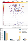 |
Fig. A.1 Top panel: Randomly selected synthetic planetary systems, sorted by stellar mass. Stars are coloured by effective temperature, and their size is based on their radius. The planets are coloured as in Fig. 2. An arbitrary scale is used for stellar radius and planet size for illustrative purposes. Bottom panel: Distribution of our generated planetary systems in the different classes defined by Mishra et al. (2021), compared to their results and to the observations (from their paper too). |
Appendix B.2 Conversion from planets mass to radius
The mass-radius relation depends on the type of planet and its composition, but it is not an exact linear relationship. To obtain an accurate global distribution while keeping a simple process of conversion, we used the relations derived by Parc et al. (2024), adding a Gaussian dispersion to reproduce the observed distribution (see eq. B.1). We randomly distributed equally planets with masses between 5 and 14 M⊕ between the first two relations.
 (B.1)
(B.1)
Appendix B.3 CDPP estimation
To estimate the effective CDPP of each planet, we used the formula of Christiansen et al. (2012): CDPPeff = √tCDPP/tdur × CDPPN, with tdur being the planet’s transit duration in hours, tCDPP the closest provided duration (3h, 6h or 12h, here we use tCDPP = 6h), and CDPPn the root-mean-square (rms) CDPP value associated with the tCDPP at the considered host star’s magnitude. We thus scaled the tabulated CDPPN to the actual duration of the transit. To do so, we need to calculate the two quantities tdur and CDPPn, as detailed below.
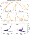 |
Fig. B.1 Comparison of host stars properties distribution, between simulated ‘detected’ exoplanet host stars (yellow histograms in top panels) and Kepler confirmed and candidate exoplanet hosts (red). Top and middle row: Magnitude, distance, effective temperature, and stellar radius distributions. Lower panels: Kiel diagrams of simulated hosts (left) and Kepler planet hosts (right). |
Assigning random inclination. As a first step, we assigned an inclination to every exoplanet’s orbit. We assumed all planets belonging to a planetary system to have the same orbital inclination. We assigned an inclination i to all host stars in our simulated Kepler field of view, following a uniform random distribution for cos(i). This leads to an average percentage of observable transits of around 2.5%.
Calculate tdur. The transit duration of an exoplanet can be defined in several ways (see Kipping (2010) for an overview). In this work, since we assumed all simulated exoplanets to have circular orbits, we chose to use the simplified expression first presented by Seager & Mallén-Ornelas (2003), with P the orbital period in hours, i the orbit inclination in degrees and aR the semi-major axis in stellar radius units:
 (B.2)
(B.2)
The computation of tdur is possible only if cos(i) ≤ aR−1.
Fitting CDPPN as a function of host star’s magnitude. The CDPPN is usually derived from the lightcurve analysis. We aim to simulate this quantity for our synthetic sample by reproducing the CDPPN distribution for Kepler Quarter 3 planetary targets, given by Christiansen et al. (2012). We fitted the distribution as a function of the magnitude for tdur = 6h. Giant stars (log(g) ≤ 4) were divided into two groups, one having higher rms CDPP, likely due to higher variability (Koch et al. 2010; Christiansen et al. 2012). We separated dwarfs from giants, sampling giant’s CDPP from the upper or lower branch randomly (half in each).
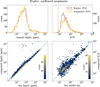 |
Fig. B.2 Comparison of calculated vs. observational transit-depth and S/N ratio distributions of Kepler exoplanets. Top panels: histograms (calculated: yellow, KOI-reported: red). Bottom panels: one-to-one comparisons. |
Appendix B.4 Transit depth and S/N comparison for Kepler confirmed exoplanets
To evaluate the accuracy of our S/N estimates, we ran the calculations detailed in Sect. B.3 for the planets detected and confirmed by Kepler. In Fig. B.2 we compare our results to the published values of Kepler Objects of Interest catalogue (KOIs). The transit depth, calculated as the square ratio of the planet’s and the host star’s radius, matches well the observational koi_depth. The median logarithmic difference between computed and koi_depth is −0.067 dex, with an absolute deviation of 0.024 dex. The planet detection S/N is obtained using equation 1. The median of log10(computed S/N) - log10(koi_model_snr) is 0.026 dex, with an absolute dispersion of 0.094 dex. We stress that the S/N is not computed for all Kepler exoplanets, because ~ 20% have an inclination not compatible with our transit duration estimation (see equation B.2).
All Tables
Planet types definitions, based on Burn et al. (2021) for masses and on Narang et al. (2018) for radii.
Main properties of the 6 simulated galaxies from NIHAO-UHD suite, compared to the MW.
All Figures
|
Fig. 1 Selection of the stellar particles of the NIHAO-UHD simulation g7.55e11 snapshot 1024 (Buck et al. 2020). Top panel: stellar particles density (number count per pixel) in Galactocentric Cartesian coordinates (in edge-on and top-down views), highlighting the selected solar neighbourhood (1147 stellar particles, highlighted in turquoise). Bottom panel: age distribution and age-metallicity relation of the selected particles, coloured by Galactocentric birth radius. Particles not belonging to the SN selection are shown in grey as reference. |
| In the text | |
|
Fig. 4 Fractions of single stars harbouring at least one planet of different planetary types. The top left panel shows the occurrence rate as a function of the stellar mass, adapted from Burn et al. (2021). The top right panel shows the occurrence rates as a function of the stellar metal-licity, adapted from Narang et al. (2018). The bottom row shows the joint occurrence rates obtained for each category of planet, combining the stellar mass and metallicity dependencies. |
| In the text | |
|
Fig. 3 Distribution of detected vs. simulated exoplanets. Left panel: detected exoplanets from the NASA Exoplanet Archive. Planets with both mass and radius measurements are shown in purple, and the ones with only mass measurements are in yellow. Planets with only radius measurement are in red (using the radius-to-mass conversions of Parc et al. 2024), but were not used to derive the bivariate Gaussian distributions. Right panel: density distribution (number count per pixel) of the 24.5 million simulated exoplanets in the solar vicinity. In grey lines are overplotted the bivariate Gaussian distributions used to assign a mass and a period to each planet randomly. The distribution of giants (HJ and CJ) and SE & Neptunes were chosen to reproduce the confirmed exoplanet population (see left panel) while the Earth-like distribution was based on the distribution predicted by (Drążkowska et al. 2023, their Fig. 13). |
| In the text | |
|
Fig. 4 All simulated exoplanets in the volume-complete SN. Influence of the planet type definition on the obtained occurrence rate, comparing three different definitions for the exoplanet categories: using the original labels, the mass or the radius. |
| In the text | |
|
Fig. 5 All simulated stars in the volume-complete SN of the g7.55e11 galactic simulation. Left panel shows the Hertzsprung-Russell diagram, colour coded by age. Right panel shows the distribution of stellar mass versus metallicity, also colour coded by age. The zoom-in panel shows the density distribution of stars in the region of the mass-metallicity space plotted in Fig. 2. |
| In the text | |
|
Fig. 6 Effective temperature of the host stars vs. instellation at the simulated exoplanet for the volume-complete SN sample. For comparison, we overplot the distribution of the observed exoplanets (Christiansen et al. 2025) as black dots and the solar-system planets as cyan diamonds. The left panel shows the entire sample, while the other three panels show the distribution of each planet category (Earth-like, SE and Neptunians, giant planets). The limits we adopted for the definition of the CHZ are plotted in dark and light green (see Sect. 3.4). |
| In the text | |
|
Fig. 7 Stellar age, mass, birth radius, and metallicity density distributions for the SN simulation. In each panel, we show the distributions of all simulated stars, stars without planets, and stars with planets, as indicated in the legend (single stars without planets represent ∼14% of the single star population). |
| In the text | |
|
Fig. 8 Summary of our simulation of the exoplanet population in the Kepler field. Upper left panel: geometric selection of stars in the simulated Kepler field, colour-coded by interstellar extinction in the G band, AG. Upper right: apparent G magnitude distribution of all simulated stars in the field of view (in blue), the ‘observable’ stars, as selected in Sect. 4.1 (green), compared to the stars observed by Kepler (Wolniewicz et al. 2021 catalogue, in red). Lower panels: transit depth and transit signal-to-noise distributions of planets in the Kepler field. Red: observed distribution among candidate+confirmed Kepler exoplanets. Green: all simulated planets with orbit inclinations compatible with a transit observation (see Sect. 4.2). Yellow: simulated detected exoplanets (i.e. planets with S/N ≥ 7.1). |
| In the text | |
|
Fig. 9 Effective temperature vs. instellation, analogous to Fig. 6, but for the simulated Kepler field. The distribution of the exoplanets observed by Kepler is shown as black dots, while the distribution of ‘detectable’ exoplanets in the Kepler simulation is shown in black density contours. The background distribution shows the distribution of planets after applying magnitude cuts described in Sect. 4.1. The number of detectable exoplanets in the simulated Kepler field is indicated on the lower left part of each panel. |
| In the text | |
|
Fig. 10 Comparison with exoplanets in the Kepler field (mass-period and radius-period diagrams). The left column shows the exoplanet population obtained by our simulation. The right plot shows the exoplanets found by Kepler (both candidates and confirmed). Top panel: planet mass (in M⊕) vs. orbital period (in days). Bottom row: planet radius (in R⊕) vs. period. For the simulated exoplanets, the radius was obtained with a conversion from the planet mass (see Appendix B). |
| In the text | |
|
Fig. 11 Results of our planetary population synthesis for different regions in the MW-like galaxy g7.55e11. Top left panels: Illustration of the regions studied, in Galactocentric Cartesian co-ordinates. Top right panels: metallicity-coloured Hertzsprung-Russell diagrams for each of the regions. Bottom left panels: Stellar age (A), stellar mass (B), birth radius (C), and metallicity (D) distributions, analogous to Fig. 7. Bottom right panel: Relative planet occurrence statistics for each of the studied regions. |
| In the text | |
|
Fig. 12 Results of our planetary population synthesis for solar neighbourhood analogues in the six publicly available NIHAO-UHD galaxies, similar to Fig. 11. The top row highlights the selections of the solar vicinity volumes (8.2 kpc from the galactic centre, see Sect. 2.1) in each of the final snapshots. Each selection, except for the more lenticular galaxy 1.12e12, contains between 2 and 4 million stars. The lower panels show the simulated stellar and exoplanet statistics and are analogous to Fig. 11. |
| In the text | |
|
Fig. A.1 Top panel: Randomly selected synthetic planetary systems, sorted by stellar mass. Stars are coloured by effective temperature, and their size is based on their radius. The planets are coloured as in Fig. 2. An arbitrary scale is used for stellar radius and planet size for illustrative purposes. Bottom panel: Distribution of our generated planetary systems in the different classes defined by Mishra et al. (2021), compared to their results and to the observations (from their paper too). |
| In the text | |
|
Fig. B.1 Comparison of host stars properties distribution, between simulated ‘detected’ exoplanet host stars (yellow histograms in top panels) and Kepler confirmed and candidate exoplanet hosts (red). Top and middle row: Magnitude, distance, effective temperature, and stellar radius distributions. Lower panels: Kiel diagrams of simulated hosts (left) and Kepler planet hosts (right). |
| In the text | |
|
Fig. B.2 Comparison of calculated vs. observational transit-depth and S/N ratio distributions of Kepler exoplanets. Top panels: histograms (calculated: yellow, KOI-reported: red). Bottom panels: one-to-one comparisons. |
| In the text | |
Current usage metrics show cumulative count of Article Views (full-text article views including HTML views, PDF and ePub downloads, according to the available data) and Abstracts Views on Vision4Press platform.
Data correspond to usage on the plateform after 2015. The current usage metrics is available 48-96 hours after online publication and is updated daily on week days.
Initial download of the metrics may take a while.