| Issue |
A&A
Volume 704, December 2025
|
|
|---|---|---|
| Article Number | A271 | |
| Number of page(s) | 16 | |
| Section | Interstellar and circumstellar matter | |
| DOI | https://doi.org/10.1051/0004-6361/202557227 | |
| Published online | 17 December 2025 | |
Globules and pillars in Cygnus X
IV. Velocity-resolved [OI] 63 μm map of a peculiar proplyd-like object
1
I. Physikalisches Institut, Universität zu Köln,
Zülpicher Str. 77,
50937
Köln,
Germany
2
Max-Planck Institut für Radioastronomie,
Auf dem Hügel 69,
53121
Bonn,
Germany
3
European Southern Observatory,
Karl-Schwarzschild-Straße 2,
85748
Garching,
Germany
4
Physikalischer Verein, Gesellschaft für Bildung und Wissenschaft,
Robert-Mayer-Str. 2,
60325
Frankfurt,
Germany
5
Laboratoire d’Astrophysique de Bordeaux, Université de Bordeaux, CNRS, B18N,
33615
Pessac,
France
6
Instituto Nacional de Astrofísica, Óptica y Electrónica,
Apartado Postal 51 y 216,
72000
Puebla,
Mexico
★ Corresponding author: This email address is being protected from spambots. You need JavaScript enabled to view it.
Received:
12
September
2025
Accepted:
3
November
2025
Abstract
A proplyd is defined as a young stellar object (YSO) surrounded by a circumstellar disk of gas and dust and embedded in a molecular envelope undergoing photo-evaporation by external ultraviolet (UV) radiation. Since the discovery of the Orion proplyds, one question has arisen as to how inside-out photo-evaporation and external irradiation can influence the evolution of these systems. For such an investigation, it is essential to determine the molecular and atomic gas masses, as well as the photo-evaporation and free-fall timescales. Understanding the dynamics within the photo-dissociation regions (PDRs) of a potential envelope–disc system, as well as the surrounding gas in relation to photo-evaporative flows, requires spectrally resolved line observations. Thus, we chose to investigate an isolated, globule-shaped object (~0.37 pc × 0.11 pc at a distance of 1.4 kpc), located near the centre of the Cygnus OB2 cluster and named proplyd #7 in optical observations. In the literature, there is no consensus on the nature of this source. Observations point toward a massive star (with or without disc) with a H II region or a G-type T Tauri star with a photo-evaporating disc, embedded in a molecular envelope. We obtained a map of the [O I] line at 63 μm with 6″ angular resolution and employed archival data of the [C II] 158 μm line (14" resolution), using the upGREAT heterodyne receiver aboard SOFIA. We also collected IRAM 30m CO data at 1 mm (11″ resolution). All the lines were detected across the whole object. The peak integrated [O I] emission of ~5 K km s−1 is located ~10″ west of an embedded YSO. The [O I] and [C II] data near the source show bulk emission at ~11 km s−1 and a line wing at ~13 km s−1, while the 12CO 2→1 data reveal additional blue-shifted high-velocity emission. The widespread [O I] emission prompts the question of its origin since the [O I] line can serve as a cooling line for a PDR or for shocks associated with a disc. From both local and non-local thermodynamic equilibrium (LTE and non-LTE) calculations, we obtained a column density of NOI ≈ 1018 cm−2 at a density of 4–8 × 103 cm−3. The [O I] line is, thus, sub-thermally excited. The KOSMA-τ PDR model can explain the emissions in the tail with a low external UV field (<350 G°, mostly consistent with our UV field estimates), but not at the location of the YSO. There, the high line intensities and increased line widths for all lines and a possible bipolar CO outflow suggest the presence of a protostellar disc. However, the existence of a thermal H II region, revealed by combining existing and new radio continuum data, points towards a massive star – and not a T Tauri-type one. The circumstellar environment of proplyd #7 consists mostly of molecular gas. We derived molecular and atomic gas masses of ~20 M⊙ and a few M⊙, respectively. The photo-evaporation (only considering external illumination) lifetime of 1.6 ± 105 yr is shorter than the free-fall lifetime of 5.2 ± 105 yr; thus, we find that proplyd #7 might not have had the time to produce many more stars. This viewpoint is supported by simulation results from the literature.
Key words: ISM: clouds / evolution / HII regions / ISM: jets and outflows / ISM: molecules / photon-dominated region (PDR)
© The Authors 2025
 Open Access article, published by EDP Sciences, under the terms of the Creative Commons Attribution License (https://creativecommons.org/licenses/by/4.0), which permits unrestricted use, distribution, and reproduction in any medium, provided the original work is properly cited.
This article is published in open access under the Subscribe to Open model. This email address is being protected from spambots. You need JavaScript enabled to view it. to support open access publication.
1 Introduction
Single low- and high-mass stars form through the gravitational collapse of magnetised cores embedded within surrounding material. The core’s initial angular momentum leads to the development of a Keplerian disc. While most of the mass accretes onto the star via the envelope and disc, a small fraction forms planets. In the earliest evolutionary stages, the material surrounding the star is gas-rich. This ‘protoplanetary disc’ is eventually dispersed by internal (central star) and external (nearby massive stars) photo-evaporation, by extreme-UV (EUV; energy >13.6 eV) and far-UV (FUV; energy between 6 and 13.6 eV) photons and X-rays (Clarke et al. 2001; Ercolano et al. 2008; Gorti & Hollenbach 2008; Alexander et al. 2014; Winter et al. 2019; Winter & Haworth 2022; Allen et al. 2025). The EUV radiation dissociates molecules and ionises atoms in the disc’s outer layers while FUV radiation mostly removes gas from the outer disc, where most of the mass is located (Gorti & Hollenbach 2009). Atomic fine structure lines, such as the neutral oxygen [O I] 63 μm line, are observed in a layer of approximately one AV within the photodissociation region (PDR) on the disc surface (Dent et al. 2013; Gorti & Hollenbach 2008). The [O I] 63 μm line is predicted to be the strongest cooling line in discs, with line luminosities as high as 10−4 L⊙ from T Tauri systems (Gorti & Hollenbach 2008; Meijerink et al. 2008; Aresu et al. 2014).
The external photo-evaporation of the disc and its enveloping molecular clump, caused by EUV and FUV radiation from nearby massive stars, was first seen in optical observations of the Orion Nebula (Laques & Vidal 1979; O’Dell et al. 1993). The discovered objects (named proplyds) appear in silhouette as discs, surrounded by teardrop-shaped envelopes with bright, ionised rims facing the exciting external source(s) and tails extending away. Follow-up observations in other regions have revealed considerable size variability among proplyds (Bally et al. 1998), with a number of them shown to be irradiated protoplanetary discs that are also still embedded in a molecular envelope; thus, such objects could feasibly be considered ‘globules’. Typical sizes for the discs of the Orion proplyds range from 45 to 355 AU, with tails that can extend up to ~2000 AU (Bally et al. 2000). Larger objects (i.e. with the size referring to the longest extent of the globule-shaped disc+envelope structure) have been identified, for example, in NGC 3603 (1.5–2.1 ± 104 AU, Brandner et al. 2000) and Cygnus (5–10 ± 104 AU, Wright et al. 2012). In Cygnus, it remains unclear if all such objects possess discs, leading Wright et al. to describe them as ‘proplyd-like’. Proplyds have also been analytically and numerically modelled (Johnstone et al. 1998; Henney & O’Dell 1999; Störzer & Hollenbach 1999; Richling & Yorke 2000; Carlsten & Hartigan 2018; Peake et al. 2025). To distinguish true proplyds from other UV-illuminated gas condensations without discs, such terms as evaporating gaseous globules (EGG; Smith et al. 2003) and globulettes (Gahm et al. 2007) have been introduced for features around 104 AU (~0.05 pc) in size. McCaughrean & Andersen (2002) proposed that either EGGs are a precursor to proplyds that eventually go on to form stars or the gas ends up completely photo-evaporating. In Schneider et al. (2016a), EGGs, globules, and proplyd-like objects in Cygnus X were classified using Herschel far-infrared (FIR) imaging at 70 μm.
Studying these objects is of particular interest, as they may represent an isolated mode of star formation, possibly regulated by gas compression driven by radiation or stellar winds. In such cases, the external compression can lead to a shortened star formation timescale. These objects are convenient to study because they exhibit a well-defined morphology and are located outside major molecular cloud complexes. Observational studies, such as the present investigation of a single object in Cygnus X (proplyd #7), together with numerical simulations, are essential for probing the interaction between protoplanetary systems and their surrounding environments. This paper is aimed at improving our understanding of the physical nature of this specific object and to contribute to our ongoing multi-wavelength studies (Schneider et al. 2016a; Djupvik et al. 2017; Schneider et al. 2021) of features such as globules, pillars, EGGs, and proplyds that have been shaped by stellar feedback.
Here, we present observations of spectrally resolved [O I] 63 μm and ionised carbon [C II] 158 μm line emission from proplyd #7 at an angular resolution of 6″ and 14″, respectively, together with complementary molecular line observations at 1 mm (Sect. 3). For simplicity, we call the whole feature, the possible disc, and the enveloping gas including the tail and proplyd (or, specifically, proplyd #7). We assume a distance of 1.4 kpc for proplyd #7 since it is most likely shaped by the Cyg OB2 association which is located at that distance (Rygl et al. 2012; Dzib et al. 2013). Previous studies, particularly Gas Survey of Protoplanetary Systems (GASPS; Dent et al. 2013) and recent investigations of proplyds in Orion and Carina (Champion et al. 2017), have relied on velocity-unresolved data obtained from the PACS spectrometer on board Herschel with a resolution of approximately 9″. By utilising the enhanced velocity resolution provided by upGREAT on the Stratospheric Observatory for Far-Infrared Astronomy (SOFIA), we can more effectively characterise the gas dynamics associated with the proplyd’s envelope (Sect. 4). However, considering the angular resolution of 6″ (corresponding to ~8400 AU at a distance of 1.4 kpc), it is not straightforward to resolve the transition between the (potential) protoplanetary disc and the surrounding envelope. We employed the FIR line and continuum data, along with the CO 2→1 observations at two positions of proplyd #7, for the PDR modeling and to independently determine the physical properties such as column densities and masses, as well as the radio SED (Sect. 5). Section 6 addresses the lifetime of this object and provides interpretations of its nature.
2 Proplyd #7 in Cygnus X
This study focuses on an object in Cygnus X classified in the infrared (IR) as IRAS 20324+4057 and by Wright et al. (2012) as a proplyd-like feature. Figure 1 shows these objects that appear in projection close to the Cyg OB2 cluster centre (Schneider et al. 2016a). The source we study here (indicated in Fig. 1 as ‘pr 7’) was previously investigated by several authors; however, its true nature remains uncertain.
Comerón et al. (2002) classified the source as a potential OB star (designated star B2), based on near-IR (NIR) spectroscopy, in particular the Br-γ line. Pereira & Miranda (2007) identified it as an H II region (source GLMP1000) with a bow shock or a disc with outflow, deduced from the observed Hα/[N II] and Hα/[S II] line intensity ratios. The ratios are more compatible with a photoionised region than a shock-excited nebulosity. Hα and [NII] images (their Fig. B.1) show that the north-western edge of proplyd #7 is particularly bright and conclude that B2 could be the (internal) exciting source. Wright et al. (2012) combined Hα, Hubble Space Telescope (HST), and Spitzer observations, named the object proplyd #7 (a term adopted in this paper) exhibiting a typical head-tail structure with a rim-brightened head. Sahai et al. (2012) further investigated this source, named it ’Tadpole’, and proposed the term frEGG (free-floating EGG). They determined that it has a length of 54.7″ (7.7 ± 104 AU, 0.37 pc) and a maximum width of 14.1″ (2.0 ± 104 AU, 0.1 pc). The size of proplyd #7 is thus at the upper end of the size range mentioned above. They identified a ‘cometary knot’ in HST images (their Fig. 2), with a peak at RA(2000) = 20h34m13.23s, Dec(2000) = 41°08′14.6″, coinciding with the location of a luminous point source in the 2MASS (20341326+4108140) and MSX6c (G080.1909+00.5353) catalogues, and with star B2 in Comerón et al. (2002). It is interpreted as scattered light from the lobes of a collimated bipolar outflow directed along the tilted, polar axis of a flared disc (or dense equatorial region). In addition, they detected three faint red stars north-west from the knot, using the High Angular Resolution Observer NIR camera on the Palomar 200-inch telescope. The VLA map of the radio emission at 8.5 GHz (Fig. 3 in Sahai et al. 2012) strongly peaks at the head of proplyd #7. The authors suggest that this is a result of a compressed magnetic layer in this front that is interacting with cosmic rays (CRs) associated with the Cyg OB2 association. From CO observations (45″ beam), they derived a mass of 3.7 M⊙ of the molecular gas around the central object; thus, they consider it more plausible that proplyd #7 is an EGG. Guarcello et al. (2013) classified the central young stellar object (YSO) in proplyd #7 as a Class I star (star 1724) from the OSIRIS (Optical System for Imaging and low-Resolution Integrated Spectroscopy) Gran Telescopio Canaria survey. In a subsequent study by Guarcello et al. (2014), the authors tentatively propose that the YSO’s spectral features are consistent with a young (<2 Myr) G-type star (T Tauri), actively accreting from a disc. They reported an intense outflow and a potential stellar jet of ionised gas, and they detected a brightness variability. They found that the mass loss rate is higher than the accretion rate and suggested that the outflow dominates. Isequilla et al. (2019) deduced from their observations at 325 and 610 MHz, using the Giant Meterwave Radio Telescope (GMRT) that the radio emission from proplyd #7 is of thermal origin, in contrast to what is stated in Sahai et al. (2012).
From the Herschel data at 36″ angular resolution, Schneider et al. (2016a) derived a hydrogen density of 8.8 × 103 cm−3, a dust temperature of 18.3 K, a size of 0.37 ± 0.11 pc (same as derived by Sahai et al. 2012), and a mass of 43 M⊙ for proplyd #7. These values refer to the disc+envelope system and the tail. Proplyd #7 is located at 5.9 pc projected distance from the Cyg OB2 association centre, commonly defined by the Cyg OB2 #8 (Schulte 1958; Wright et al. 2015) trapezium of O stars. It has been suggested (Wright et al. 2012; Guarcello et al. 2014) that the morphology and orientation of proplyd #7 (and other objects in this region) are governed by the stellar feedback from Cyg OB2 #8. However, Isequilla et al. (2019) favour the O-stars Cyg OB2 #9 and #22 as the dominating ionizing sources. The closest system to proplyd #7 are three B-stars of type B0.5 V, B 1.5 V, and B1V. We derive and discuss the UV field in this paper.
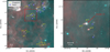 |
Fig. 1 False-colour image of the central Cygnus X region (left; Schneider et al. 2016a) and a zoom onto the region indicated by the red dashed box around Proplyd #7 (right). The R and G channels correspond to Spitzer 8 μm, while the B channel corresponds to Herschel (PACS 70 μm) emission. The proplyd-like objects detected by Wright et al. (2012) and Schneider et al. (2016a) are labelled in yellow (pr1-11). Proplyd #7 (pr 7) is located in the upper centre region, close to some massive stars of the Cyg OB2 association. These are marked in grey, following the nomenclature in Wright et al. (2015). |
3 Observations
3.1 SOFIA
The [O I] atomic fine structure line at 4.74478 THz (63.2 μm) and the CO 16→15 rotational line at 1.841345 THz were observed with the heterodyne receiver upGREAT1 on board SOFIA during one guaranteed time (GT) flight on 2 November 2016, from Palmdale, California (programme ID 83_0433). The [O I] line was observed in the 7-pixel High Frequency Array (HFA), and the CO line in the one-pixel L 2 channel. The map centre position is RA(2000)=20h34m13.3s and Dec(2000)=+41°08′13.8″. The observing mode was set to on-the-fly (OTF) mapping with chopping in single phase A with a chop throw of 120″ and a chop frequency of 0.655 Hz. The array orientation was tilted by −19.1 deg relative to the scanning direction so that the HFA 7 pixels scan at an equal distance. The central channel was set to a velocity of +8 km s−1. The map covers an area of ~60″×30″.
Procedures to determine the instrument alignment and telescope efficiencies, antenna temperature, and atmospheric calibration, as well as the spectrometers used are described in Heyminck et al. (2012) and Guan et al. (2012). All line intensities are reported as main beam temperatures scaled with main-beam efficiencies of 0.69 and 0.68 for [O I] and CO, respectively, and a forward efficiency of 0.97. The main beam sizes are 6.1″ for the H-channel and 15.3″ for the L2 channel.
The calibrated [O I] and CO spectra were further reduced and analysed with the GILDAS software, developed and maintained by IRAM. From the spectra, a third-order baseline was removed and spectra were then averaged with 1/σ2 weighting (baseline noise). The mean rms (root mean square) noise temperatures per 0.28 km s−1 velocity bin is 0.8 K for [O I] in a 6″ beam. The CO 16→15 line was not detected on a 0.4 K rms level in a velocity bin of 0.6 km s−1. We estimate that the absolute calibration uncertainty is around ~20%. The telluric [O I] line, originating from the mesosphere, is visible in the spectra as an absorption feature, but is located at +1 km s−1 and, thus, far away from the systemic velocity of the proplyd, which is around 11 km s−1.
We also used [O I] 63 μm and [C II 158 μm line data from the SOFIA archive, collected as part of programme 05_0176 (PIs: R. Sahai et al.), obtained with the HFA and LFA-array of upGREAT (Risacher et al. 2018). The spectra had a baseline of an order of one removed in terms of the fixed velocity scale and they were also sigma-weighted during the averaging of spectra per position. The beam efficiencies were determined for all HFA (LFA) pixels (varying between 0.59 and 0.68 for the HFA array) and between 0.65 and 0.73 for the LFA array using Jupiter as a calibrator and applied individually. All [O I] and [C II] temperatures are thus in main beam brightness temperatures and the beam size is 14.1″ for [C II] and 6.1″ for [O I]. We note that only a single footprint of the arrays was obtained for proplyd #7 and not a full map in [O I] as for our GT data set. A complementary set of publicly available data were used for this study, including Herschel and Spitzer.
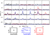 |
Fig. 2 [O I] 63 μm, [C II] 158 μm, and 12CO 2→1 spectra of proplyd #7. To increase the S/N, the [O I] data were smoothed to an angular resolution of 10″ and re-gridded to 10″ (original resolution 6″ on a ~2″ sampling grid). The velocity resolution was degraded to ~0.4 km s−1. The [C II] (CO) spectra are on their nominal angular resolution of 14″ (12″) and velocity resolution of 0.2 (0.3) km s−1. The displayed main beam brightness temperature and velocity ranges are indicated in the small lower panels. The star indicates the approximate location of the YSO. |
3.2 IRAM 30m
Proplyd #7 was observed for 2 h within Director’s Discretionary Time (DTT) in a setting at 1 mm (tuning frequency 218.6 GHz) with EMIR, covering the following lines: 12CO (230.538 GHz), 13CO (220.3987 GHz), and C18O 2→1 (219.560 GHz), as well as other molecular lines such as SiO 5→4, DCO+ 3→2, and DCN 3→2, and two H2CO lines. All data have an angular resolution of 11–12″. Here, we present only the isotopomeric CO 2→1 data. We started by observing a strip with four pointings and then performed an OTF map that is 120″×80″ in size, with one horizontal and one vertical coverage, respectively. The weather conditions were good (opacity at 1 mm 0.3 to 0.4) and the pointing accuracy was checked with the source K3-50A and found to be good within 1–2″.
3.3 GLOSTAR
We made use of radio continuum data from the Global View of Star Formation in the Milky Way (GLOSTAR) survey (Medina et al. 2019; Brunthaler et al. 2021), which combines data taken at the Karl G. Jansky Very Large Array (VLA) in its D and B-configurations with zero-spacing from the Effelsberg 100 m telescope. The correlator setting covers the continuum emission in full polarization within 4–8 GHz (using two 1 GHz sub-bands centred at 4.7 and 6.9 GHz). For technical details, we refer to the papers cited above. Here, we used data in a combined B +D configuration with a resolution of 4″. The mean background level, as determined in an emission-free region north-west of proplyd #7, is 0.2 mJy.
4 Results
4.1 [OI], [CII], and CO line observations
Figure 2 presents the observed [O I], [C II], and CO 2→1 spectra across proplyd #7. The [O I] line is prominently detected, with peak emission around the (0,0) position, very close to the location of the YSO. Notably, strong [O I] emission is also observed in the proplyd tail (1.6–1.9 K). However, to thermally excite bright [O I] 63 μm emission densities of a few 105 cm−3 and high temperatures (typically >100 K) are required. As we will see later, these conditions are not given in the proplyd tail. The [C II] observations tend to feature fewer data points, but they do exhibit a similar spatial distribution for the emission. In the proplyd tail, all lines display a single Gaussian component with a peak velocity around 10.5 km s−1. In contrast, the spectra around the (0,0) position require a fit with at least two2 Gaussian components (an additional component at ~13 km s−1), an example for a fit to the [O I] line at offset (−4″, 0) is displayed in Fig. 3. The red-shifted wing is seen in all lines and most likely indicates gas streaming away from the observer. Although low-mass stars often exhibit outflow signatures during their early evolutionary stages driven by accretion processes in the disc, with previous studies, such as Guarcello et al. (2014), indicating outflow activity, it is unlikely that the 13 km s−1 component represents a highly collimated [O I] jet. This is because typical [O I] jets have velocities exceeding 100 km s−1 (Podio et al. 2012). However, for massive stars (Kuiper et al. 2011), an envelope-disc interaction leads to an atomic jet of at least partly ionised gas orthogonal to the disc, which can then drive a molecular outflow (see below) and create an outflow-confined H II region. The [O I] velocities can be lower, but still of the order of a few 10 km s−1 and thus also faster than the velocity difference we observe for the wing emission with respect to the bulk emission.
Another possibility is that the red-shifted [O I], [C II], and CO emission is due to a photo-evaporative flow, triggered by external UV radiation. Proplyd #7 is clearly exposed to the radiation and wind of the nearby O-stars (Sect. 5.1) and we could expect a dynamic impact with gas released from the surface layer. This would explain the small difference in velocity between the bulk emission and the red-shifted wing emission. However, the atomic and molecular line profiles across proplyd #7 do not show broad wings everywhere, which would be expected in the case of significant photo-evaporation. We note that this can be a geometry effect, combined with the low angular resolution. In the case where the closest star #720 (see Sect. 5.1) would have the largest influence on proplyd #7, the radiation field and wind would be strongest at the western border, which is only approximately two beam sizes away from the YSO. The tail extends further east from the YSO and is thus shielded from direct stellar irradiation.
Table 1 presents the [O I] line fitting results and associated errors for both spectral components. Only positions where the main beam brightness temperature exceeds the rms noise are included, as indicated in the table. However, some results have substantial uncertainties and should be interpreted with caution. Figure 5 displays maps of the line centre velocity and width overlaid on a colour plot of PACS 70 μm emission, with line-integrated (9–14 km s−1) [O I] emission contours. The peak of [O I] emission is offset by approximately 6″ to the west of the YSO and the 70 μm peak, which marks the location of hot dust heated by the central star3. A similar distribution is evident in the Spitzer/IRAC image at 8 μm (Fig. 6).
From Fig. 5, a clear gradient in line velocity and width of the first component is observed, extending from east to west along proplyd #7. The central velocity decreases from 11.3 km s−1 at the western edge to 10.5 km s−1 at the eastern end of the tail. The line width of the main component 1 is approximately 1.1 km s−1 near the western border, increases significantly at the position of the YSO to 2.37 km s−1 and gradually decreases to 1.27 km s−1 in the tail. The elevated line width at the central position, combined with the presence of a high-velocity wing in [O I] emission, suggests a significant role for the central star’s radiation in producing the observed [O I] emission (see discussion above). If the [O I] 63 μm line was mainly driven by the externally illuminated PDR, such a marked variation in line width would not be expected. If the central source is a massive star with a (compact) H II region, the interaction of the radiation and wind of the source with the interface (i.e. the atomic PDR and then the molecular envelope) could result in high-velocity emission in all line tracers ([O I], and [C II] in the PDR and CO in the molecular gas) without the need of an accretion disc. If there is an accretion disc (regardless if the central source is a T Tauri or a massive star), the high accretion luminosity could be the source for the [O I] excitation by shocks though accretion luminosity is also often released in the UV and then leads to a second internal PDR. This would superimpose the shock effect. The [O I] (and possible [C II]) emission would then arise from the photoevaporating disc. However, we did not detect emission4 from a shock tracer (SiO 5→4) and the observed velocity gradient across the proplyd is also not straightforward to explain in this scenario.
Results from fitting two Gaussian lines to the observed [O I] spectra.
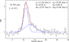 |
Fig. 3 Example of an [O I] spectrum and fit to the data. The black histogram shows the observed [O I] spectrum closest to the central YSO (position with offset −4″,0), smoothed to an angular resolution of 10″. The blue Gaussian lines represent the fit to this spectrum with two components. Centre velocity, temperature, and FWHM values are given in the panel. The red line gives the resulting fit. |
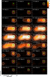 |
Fig. 4 Channel map of 12CO 2→1 line emission. Each channel covers a velocity range of 0.3 km s−1. Contours go from 2 to 34 K km s−1 in steps of 4 K km s−1 and the green star indicates the position of the YSO. |
4.2 A protostellar CO outflow
A CO 2→1 bipolar outflow, oriented apparently mostly along the line of sight, is clearly identifiable in the channel maps of CO emission shown in Fig. 4 (channel maps of 13CO and C18O 2→1 emission are given in Fig. A.1), and in the 3D position-velocity (PV) cut in Fig. A.2. Both, the blue-shifted (~7–9 km s−1) and the red-shifted (~11–14 km s−1) components appear rather focussed on the central source. One possibility is that we are observing a protostellar outflow from a young star with an accretion disc that lies mostly in the plane of the sky. This is in tension with the proposal of Sahai et al. (2012), who interpreted a conical optical feature as scattered light from an outflow, tilted in a way so that the near-side of the disc is lying to the north-west of the YSO. They derived an opening angle of the bipolar outflow cavity around 5–7° and an outflow cavity axis inclined at an angle of 18° to the line of sight. Because of the low angular resolution of our CO data, we could exclude this geometry, but we do note that comparing the CO outflow and the optical observations is challenging. Whether the central source is a low-mass star, a G-type star (T Tauri) as proposed by Guarcello et al. (2014) or a massive young star can also not be concluded from the CO observations alone.
Another possibility for the outflow emission is that a massive star (with or without disc) has created a cavity by its radiation and winds and entrained gas can also arise from ablation of gas at the cavity borders to the surrounding molecular cloud (see Sect. 4.1). This scenario was previously reported, for example, in S106 (Schneider et al. 2018) and in a globule in Cygnus X (Djupvik et al. 2017; Schneider et al. 2021).
4.3 GLOSTAR observations
Figure 7 displays the GLOSTAR image of proplyd #7 at 5.9 GHz, determined from the B+D VLA configuration at 4″ angular resolution. The radio emission distribution is similar to what was observed at 8.5 GHz and 22 GHz (Sahai et al. 2012). Firstly, the emission forms a bright half-circle at the western head of proplyd #7. This appearance can have various explanations. It can be caused by higher density due to external compression (radiation and wind from the close-by OB-stars). However, it is also possible that the YSO is a massive star and created a compact H II region, where the expanding ionised gas is compressed from the inside and forms a denser and, thus, brighter shell in the west while towards the east, dense molecular gas forms a barrier. This scenario would well explain the half-circle morphology. No very compact emission was detected in the GLOSTAR B-configuration which is sensitive to structures up to 4″, that correspond to 0.03 pc at a distance of 1.4 kpc. This could imply that we do not observe an ultra-compact H II region (sizes of <0.1 pc), but moreover a more evolved, compact H II region that is typically 0.1–0.5 pc in size, depending on density.
The large-scale 5.9 GHz emission can have several reasons. It is clear that enough EUV photons are required to generate the ionised hydrogen for the free-free emission. Proplyd #7 could be embedded in an environment with a sufficient large fraction of ionised gas. We checked the Cygnus mapping at 1′ resolution of the Canadian Galactic Plane survey (Taylor et al. 2003) at 1420 MHz and indeed reveal that there is an enhanced level of ~12 mJy emission around proplyd #7. Figure 8 in Setia Gunawan et al. (2003) shows also a higher emission level around proplyd #7 (their source 118). Another argument for external illumination is that all other proplyd-like objects in this area also shine at 5.9 GHz, even those who clearly do not have an internal YSO.
Nevertheless, it is also possible that EUV photons stem from inside. In this case, the central YSO must be a massive star (see above) with an internal H II region and the material east of the bright emission spot must be very clumpy so that the EUV photons can channel through the molecular clump. Proplyd #7 has a fragmented structure, this becomes obvious in the overlay with line integrated 13CO emission (lower panel of Fig. 7) and in the channel maps displayed in Fig. A.1. However, higher angular resolution molecular line observations are necessary to better reveal the structure.
From the drop in flux between 8.5 GHz and 22 GHz, Sahai et al. (2012) argued in favour of non-thermal emission (Fig. A.3 displays the radio SED). However, the observed flux density at 5.9 GHz is at around 49 mJy and, thus, it is significantly lower than what would be expected from purely non-thermal emission, indicating an optically thick regime consistent with a thermal H II region; meanwhile, the 22 GHz emission is in the optically thin part of the SED. We note that the flux density at 22 GHz is a lower limit because these observations were performed in the C-configuration and even though an UV-taper was applied to arrive to a similar beam as for the 8.5 GHz observations, the shorter baselines are missing at 22 GHz so that extended emission gets lost. In summary, from the overall emission distribution (Fig. A.3) and the comparison between the absolute values of radio emission, we deduced that we observe typical free-free emission from a thermal compact H II region. This conclusion is similar to what was stated in Isequilla et al. (2019), described with a turnover frequency of a few GHz.
 |
Fig. 5 Distribution of [O I] line centre velocity and FWHM. Overlays of [O I] line integrated (v=9 to 15 km s−1) emission (contour levels 5, 6, 7, 8, and 8.5 K km s−1) on Herschel/PACS 70 μm emission in color. The left panel shows the line centre velocities in km s−1 of the two components (first component in black, second in grey) and the right panel the linewidth in km s−1. The values (Table 1) were determined from Gaussian fits to the spectra from Fig. 2. |
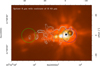 |
Fig. 6 Spitzer 8 μm image of proplyd #7. The NIR map is in units of MJy/sr, ranging from 44 to 1.4 ± 104 with contours of [O I] emission (5, 6, 7, 8, 8.5 K km s−1) overlaid. Two positions where the PDR modelling was performed are indicated: position 1 (offset −4″,0) with a blue circle (radius 7″) and position 2 (offset 36″, 0) with a green circle, respectively. |
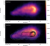 |
Fig. 7 GLOSTAR 5.9 GHz images of proplyd #7. The top image shows the GLOSTAR data only. The image scale is in Jy/beam at an angular resolution of 4″. The star indicates the position of the YSO. The lower panel displays the same radio image with contours of 13CO 2→1 emission overlayed. The contour lines have values of 5–37.5 K km s−1 in steps of 2.5 K km s−1. |
5 Analysis
5.1 The external FUV field of proplyd #7
A central question in revealing the nature of proplyd #7 is to assess how much of the observed emission in all line tracers is caused by internal and external radiation. Given that proplyd #7 is oriented towards the centre of the Cyg OB2 association, its morphology was most likely influenced by external stellar feedback. Pereira & Miranda (2007) and Wright et al. (2012) showed in their Hα maps that the northern edge of proplyd #7 is brighter than the southern part, suggesting an influence from the central O-stars of Cyg OB2 (mainly #8, 9, and 22 from the notation of Schulte (1958). However, the overall orientation of proplyd #7 is west-east and points mostly towards the star #720 (notation from Massey & Thompson 1991; see our Fig. 1). Figure 8 (Schneider et al. 2016a) displays the FUV field, obtained by translating the observed Herschel 70 and 160 μm fluxes into a FUV field, assuming all incoming radiation is re-radiated in the FIR. We note that it is clear that a FUV field can only be determined in this way when there is enough material so that all FUV photons can be absorbed in a PDR. Otherwise it provides a lower limit only. We obtained values of 352 and 239 G° for positions 1 and 2, respectively and a high field of 1737 G° at the location of the YSO. From the stellar census5, Schneider et al. (2016a) derived an upper limit of ~1000 G° averaged over proplyd #7. Because at the position of the YSO we find a significantly higher value, it is obvious that there is additional heating (potentially through an internal PDR).
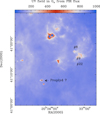 |
Fig. 8 FUV field around proplyd #7. The FUV field in Habing units (G°) is determined from the Herschel 70 and 160 μm fluxes on an angular resolution and on a grid of 11". Proplyd #7 is indicated by an arrow. |
5.2 PDR (photodissociation region) modelling
We employed KOSMA-τ (Röllig et al. 2006; Röllig & Ossenkopf-Okada 2022), a well-tested (Röllig et al. 2007) PDR model to derive local physical conditions from the observed [O I], [C II] and CO 2→1 line intensities and ratios, and FIR 70 and 160 μm fluxes.
KOSMA-τ numerically computes the energetic and chemical balance in a spherical cloud with a density gradient similar to a Bonnor–Ebert sphere that is externally irradiated. The whole region is represented by an ensemble of such spherical clumps. While the model allows for superpositions of different clumps with a size spectrum, we only used the simplified approach with identical clumps sizes. The full numerical computation scheme of KOSMA-τ involves three steps.
First, the continuum radiative transfer code MCDRT (Szczerba et al. 1997) was used to compute the thermal balance of all dust components as well as the FUV radiative transfer within the model cloud, and the emergent continuum radiation. We employed the dust model 7 from Weingartner & Draine (2001a), which assumes that the impact of the gas on the dust temperature is negligible. The MCDRT output was then used as input for the second step, where KOSMA-τ computes the chemical structure and temperature of the gas in equilibrium. The result are radial chemical and temperature profiles of the model clump. In a third step, they are used to perform the line radiative transfer computations, giving the spectral emission of the model cloud for comparison with observations (Gierens et al. 1992). In the model runs, we applied the most recent CO self-shielding functions by Visser et al. (2009) and assume a Doppler line width according to the line width-and-size relation by Larson (1981). The photoelectric heating is estimated according to Weingartner & Draine (2001b). The formation of H2 on grain surfaces follows Cazaux & Tielens (2002, 2004, 2010) and formation on PAH surfaces is suppressed. We applied the UMIST Database for Astrochemistry chemical network (McElroy et al. 2013), including all isotopic reaction variants including 13C and 18O isotopes. More details on the model and how it is applied to SOFIA data can be found in Schneider et al. (2018, 2021).
In Table 2, we give the values of the [O I], [C II], and CO 2→1 line intensity for two positions where we performed the modelling processes indicated in Fig. 6. Position 1 (−4″,0″) characterises the peak of [O I] emission and is close to the location of the YSO, while position 2 (36″,0′) is in a more quiescent region in the tail of proplyd #7. The upper limit for the mass for both positions in one beam is around 2 M⊙, determined from the Herschel column density map. Thus, we used the KOSMA-τ models that were calculated for a clump mass of 1 M⊙; however, we note that the model results depend only weakly on the clump mass.
The [O I] line integrated (over the whole velocity range) intensity is 5.8 × 10⁻⁴ erg s−1 sr−1 cm−2 and 1.6 × 10⁻⁴ erg s−1 sr−1 cm−2 for positions 1 and 2, respectively. These values are lower than what was observed for the proplyds in Carina (4.5 × 10⁻³ erg s−1 sr−1 cm−2) and Orion (1.5 × 10⁻² erg s−1 sr−1 cm−2) by Champion et al. (2017).
Figure 9 presents the parameter space of gas density and FUV radiation field derived from the KOSMA-τ model (2020), implemented in the PDR Toolbox (Pound & Wolfire 2023) as ‘non-clumpy’. The intersection of the observed line intensities and diagnostic line ratios delineates the most probable values for both the gas density and the FUV field strength. From the plots, it becomes obvious that the PDR model does not deliver one simple solution for the density and UV-field for the two positions. For position 1, the FIR line emission and ratios indicate a FUV field <100 G°) that is lower than the one estimated from the FIR flux-based method. The Herschel flux values of 70 and 160 μm cover a parameter space with much higher FUV field. The derived gas density has values of the order of 105 cm−3, which is consistent with expectations for dense PDRs.
For position 2, the FIR lines point towards an even lower FUV field (around 20 G°) and a density of 104 cm−3, while the Herschel flux values and the 12CO 2→1 line cross approximately the estimated field of around 240 G° at a density of 104 cm−3. In addition, the PDR model delivers a surface temperature of around 150 to 200 K.
The inconsistency between the fit results for the line and continuum data suggests that the chemical and thermal structure of proplyd #7 are governed by several processes and not by FUV radiation alone. Considering only the effect of photo-dissociation, the actual PDR chemistry is traced through the [O I] and [C II] lines where the observations suggest a relatively low FUV field. In contrast the thermal dust emission traces the total energy input into the ISM, including compression, shocks, magneto-hydrodynamic (MHD) dissipation, and radiation outside of the FUV wavelength range. The fact that the continuum levels suggest much higher radiation fields in the fit indicates that those non-FUV processes are dominant in proplyd #7 (at least at the position of the YSO), so that it cannot be described as a simple PDR. Nevertheless, the model is useful to constrain the gas density and assess the pure FUV effect.
Values for the PDR modelling.
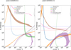 |
Fig. 9 PDR KOSMA-τ model results. The left (right) panel shows the diagnostic diagrams for UV-field and density, derived from the observed lines, line ratios, and FIR fluxes for positions 1 and 2 in proplyd #7. The red and blue dashed lines indicate the UV field determined from the FIR Herschel fluxes and from the stellar census, respectively, for positions 1 and 2. |
5.3 The physical properties and star-formation history of proplyd #7
We used the CO data to determine the excitation temperature and column densities (NCO and N(H2)) across proplyd #7 as well as to estimate the total molecular gas mass. The FIR [O I] 63 μm and [C II] 158 μm lines were used to derive the mass of the atomic gas component associated with the PDR of proplyd #7. Detailed calculations are given in Appendix B and we also summarise these results in Table 3. We note that all values are an approximation and have significant uncertainties (see Appendix B). The total mass is an important property because it determines its evolution and lifetime and, thus, the total time available for accretion by the star(s) that might form inside it and for any further stars that might subsequently form.
The molecular mass derived from CO observations is 16.3 M⊙, which is comparable to the 19.1 M⊙ obtained from the Herschel column density map that includes both atomic and molecular hydrogen (see column 4 in Table 3). In contrast, the atomic gas mass is significantly lower, with 1.8 M⊙ and 3.9 M⊙, derived from [O I] and [C II] emission, respectively. Thus, the atomic PDR associated with proplyd #7 contributes only a minor fraction to the total mass. The mass-loss rate is estimated using Eq. (3) from Schneider et al. (2016a), adopting the same values for the external UV photon flux, the equivalent radius, and the distance to the central stars of Cygnus OB2. This yields a mass-loss rate of 9.65 × 10⁻⁵ M⊙ yr−1, at least a factor 100–1000 larger than the typical values for the Orion proplyds (Henney & O’Dell 1999; Sheehan et al. 2016; Winter et al. 2019; Ballering et al. 2023; Aru et al. 2024; Boyden et al. 2025). The photo-evaporation time (tphoto), defined as the time required to completely photo-evaporate the object (assuming constant density but a variable radius), is calculated using Eq. (4) in Schneider et al. (2016a), resulting in tphoto = 1.62 × 10⁵ yr. We adopted the UV exposure time for proplyd #7 as texpos = 4.52 × 10⁶ yr, based on Table A.2 of Schneider et al. (2016a). The free-fall time for an isothermal, gravitational collapse is computed using the standard expression ![Mathematical equation: $\[\mathrm{t}_{f f}=\sqrt{\left(3 \pi /(32 G~ n~ m_{H} ~\mu)\right.}\]$](/articles/aa/full_html/2025/12/aa57227-25/aa57227-25-eq1.png) , where G is the gravitational constant, n = 4.4 × 103 cm−3 is the average particle number density, mH is the mass of a hydrogen atom, and μ = 2.33 is the mean molecular weight accounting for the presence of heavier elements. We obtain a value of tff = 5.2 × 10⁵ yr. The photo-evaporation timescale is relatively short, 1.62 × 10⁵ yr, consistent with values derived for the proplyds in Orion (Johnstone et al. 1998). In contrast, the free-fall timescale is more than twice as long, indicating that proplyd #7 is likely to be dispersed by external irradiation before it can undergo gravitational collapse and form more stars. The lifetime of proplyd #7 is probably even shorter if we consider the feedback effects (radiation and wind) from the internal YSO.
, where G is the gravitational constant, n = 4.4 × 103 cm−3 is the average particle number density, mH is the mass of a hydrogen atom, and μ = 2.33 is the mean molecular weight accounting for the presence of heavier elements. We obtain a value of tff = 5.2 × 10⁵ yr. The photo-evaporation timescale is relatively short, 1.62 × 10⁵ yr, consistent with values derived for the proplyds in Orion (Johnstone et al. 1998). In contrast, the free-fall timescale is more than twice as long, indicating that proplyd #7 is likely to be dispersed by external irradiation before it can undergo gravitational collapse and form more stars. The lifetime of proplyd #7 is probably even shorter if we consider the feedback effects (radiation and wind) from the internal YSO.
Physical overall averaged properties of proplyd #7.
6 Conclusions: Proplyd #7 as an embedded protoplanetary disc or an irradiated globule
Our millimetre (mm), FIR, and radio observations of proplyd #7 are limited by angular resolution, ranging from 4″ to 14″, which hampers the ability to disentangle emission from a potential protoplanetary disc and the molecular envelope. The embedded YSO within proplyd #7 may still be accreting mass from the surrounding gas reservoir. This scenario contrasts with that of typical Orion proplyds, where the disc is actively losing mass due to external photo-evaporation. Despite these limitations, we detected outflow signatures in the CO, [O I], and [C II] lines near the location of the YSO. These emissions could originate from two plausible scenarios:
(i) a protoplanetary disc associated with the central star, either a massive star or a T Tauri star.
(ii) gas ablated from the cavity walls by the radiation and stellar winds of a massive central star in the absence of a disc.
Both scenarios are possible; however, scenario (ii) is more probable, mostly because of the radio continuum observations that point toward the existence of a thermal H II region and stellar classifications in the literature (Comerón et al. 2002; Isequilla et al. 2019), which suggest that the central object is an OB star. In this case, the [C II] and [O I] lines may be shock-excited, explaining why the observed line intensities and FIR continuum fluxes deviate from the KOSMA-τ PDR model predictions. The CO emission is likely entrained in the ionised outflow. This would explain the contradiction why the FIR continuum emission in proplyd #7 is reasonably well reproduced by an external UV radiation field of a few hundred G0 (at least for position 2), but the observed [O I] and [C II] line intensities are better matched by models assuming a lower FUV field. However, the situation is more complex. We observe the same morphology in dust, radio continuum (that we interpret as thermal), and CO, which is inconsistent because on one hand, EUV photons need to penetrate for the free-free emission; however, FUV shielding is required for the formation of CO. Having both in the same structure is only possible if we have a very clumpy medium with dense, self-shielding clumps and a highly fragmented structure with many channels for UV penetration in between. However, in this case, we tend to run into problems for the calculation of the FUV field. The FUV estimate from the FIR emission assumes that all FUV photons are absorbed; thus, accordingly, we cannot have too many leaking photons (i.e. there is a margin of about a factor 2 when looking at the numbers). However, the EUV extinction should exceed the FUV extinction. Therefore, it is unclear how we can manage to still have enough EUV photons to generate all the ionised hydrogen required for free-free emission. This is only possible if proplyd #7 was indeed found to be embedded in a significantly ionised medium, which is not fully the case (Sect. 4.3).
Overall, the external irradiation from nearby OB stars in the Cyg OB2 cluster may have had only a moderate impact on proplyd #7. The object has been exposed to UV radiation for approximately 4.5 × 10⁶ yr and has persisted over this timescale. It remains uncertain whether the formation of the central star(s) resulted from radiative and wind-driven gas compression by the OB stars or from spontaneous gravitational collapse of an isolated molecular clump. The Jeans mass6 is a few M⊙ for typical temperatures of 10–20 K and densities 103 to 104 cm−3 and, thus, much lower than the current gas mass of ~20 M⊙, as derived from CO and dust (the initial cloud mass was likely higher). In contrast, the atomic gas mass (estimated from [O I] and [C II] emission) is relatively low, on the order of a few M⊙. From a simulation viewpoint, the ongoing star formation within proplyd #7 has not necessarily been triggered externally (e.g. by a shock front preceding a D-type ionization front). Smooth particle hydrodynamic simulations presented in Bisbas et al. (2011), which model the propagation of ionizing radiation and the resulting dynamical evolution of a molecular clump, show in their Fig. 12 a parameter space of ionizing flux and clump mass that distinguishes between regimes of triggered star formation and clump dispersal. Proplyd #7 has an upper limit for the ionizing flux of 4.8 × 1010 cm−2, estimated from a geometric dilution factor of 1/(4πd2) at a distance, d, of 5.9 pc from the central Cyg OB2 cluster, assuming a photon emission rate of 1050.3 s−1 (Schneider et al. 2016a). With a mass of ~20 M⊙ (Table 3), this places proplyd #7 within the regime where the clump is expected to be dispersed rather than to undergo externally triggered star formation through mechanisms such as radiatively driven implosion (Lefloch & Lazareff 1994). This is supported by arguments of timescales. Proplyd #7 is unlikely to survive much longer because given its photo-evaporation timescale of 1.62 × 10⁵ yr and a free-fall time of 5.2 × 10⁵ yr, it is improbable that further star formation will occur within this object.
Although significant progress has been made in understanding the nature of proplyd #7, further observations are required to address the key question of whether we are observing a disc around a massive star within a globule (a remarkable discovery if confirmed) that is driving a protostellar CO outflow. NIR spectroscopy and imaging of H2 and Brγ emission from the central object would aid in determining the spectral type of the potential massive star. However, this is most likely not possible because the spectrum of the central star is strongly veiled, as demonstrated in Guarcello et al. (2014). One could use for example the James Webb Space Telescope (JWST) to observe CO vibrational bands to trace the hot and cold gas and light hydrocarbons. H2 NIR (NIRSpec) observations could provide a much better understanding of the distribution of the molecular gas. New FIR cooling line observations are no longer possible following the shutdown of SOFIA; however, the [O I] 63 μm line emission, together with [C II] emission and hydrogen column densities, can be incorporated into shock models such as the Paris-Durham model (Godard et al. 2019). However, this analysis lies beyond the scope of the present work. Such modelling would reveal whether the relatively strong [O I] and [C II] emissions originate from protoplanetary disc environments where shocks and high-energy processes occur. These processes could include accretion shocks arising from gas infall onto the central star, heating of the inner disc regions that induces shocks, or jet-driven shocks generated either by outflows from the central star or by interactions within the disc that propagate into the surrounding medium. On the other hand, [O I] emission arising from an atomic jet linked to the disc-envelope-star system is predicted to emerge from high-velocity (≪100 km s−1) dissociative J-type shocks that hit the dense surrounding gas (Hollenbach 1985; Hollenbach & McKee 1989). In contrast, the observed redshifted [O I] emission exhibits relatively low projected velocities of ~2–5 kms−1.
In summary, proplyd #7 retains unresolved characteristics and apparent contradictions that warrant further investigation. It remains uncertain whether proplyd #7 truly merits its designation as a protoplanetary disc or whether it is instead a compact, small globule undergoing internal star formation. However, the study presented here sets constraints on the timeline of the evolution of this object and highlights observational discrepancies that future higher angular resolution studies have to solve.
Acknowledgements
We thank the anonymous referee for very useful comments. This study was based on observations made with the NASA/DLR Stratospheric Observatory for Infrared Astronomy (SOFIA). SOFIA is jointly operated by the Universities Space Research Association Inc. (USRA), under NASA contract NNA17BF53C, and the Deutsches SOFIA Institut (DSI), under DLR contract 50 OK 0901 to the University of Stuttgart. (up)GREAT is a development by the MPI für Radioastronomie and the KOSMA/Universität zu Köln, in cooperation with the DLR Institut für Optische Sensorsysteme. This work partially uses data from the GLOSTAR survey, whose database is available at http://glostar.mpifr-bonn.mpg.de and is supported by the MPIfR, Bonn. N.S. acknowledges support by the BMWI via DLR, Projekt Number 50OR2217. S.K. acknowledges support by the BMWI via DLR, project number 50OR2311. This work was supported by the CRC1601 (SFB 1601 sub-project A6, B2) funded by the DFG (German Research Foundation) – 500700252. S.D. acknowledges support by the International Max Planck Research School (IMPRS) for Astronomy and Astrophysics at the Universities of Bonn and Cologne. S.A.D. acknowledges the M2FINDERS project from the European Research Council (ERC) under the European Union’s Horizon 2020 research and innovation programme (grant No. 101018682). G.N.O.L. acknowledges the financial support provided by Secretaría de Ciencia, Humanidades, Tecnología e Innovación (Secihti) through grant CBF-2025-I-201. We thank the director of IRAM, Karl Schuster, for providing us with Director’s Discretionary Time to observe proplyd #7 with the IRAM 30m telescope.
References
- Alexander, R., Pascucci, I., Andrews, S., Armitage, P., & Cieza, L. 2014, in Protostars and Planets VI, eds. H. Beuther, R. S. Klessen, C. P. Dullemond, & T. Henning, 475 [Google Scholar]
- Allen, M., Anania, R., Andersen, M., et al. 2025, Open J. Astrophys., 8, 54 [Google Scholar]
- Aresu, G., Kamp, I., Meijerink, R., et al. 2014, A&A, 566, A14 [NASA ADS] [CrossRef] [EDP Sciences] [Google Scholar]
- Aru, M. L., Maucó, K., Manara, C. F., et al. 2024, A&A, 687, A93 [NASA ADS] [CrossRef] [EDP Sciences] [Google Scholar]
- Ballering, N. P., Cleeves, L. I., Haworth, T. J., et al. 2023, ApJ, 954, 127 [NASA ADS] [CrossRef] [Google Scholar]
- Bally, J., Sutherland, R. S., Devine, D., & Johnstone, D. 1998, AJ, 116, 293 [NASA ADS] [CrossRef] [Google Scholar]
- Bally, J., O’Dell, C. R., & McCaughrean, M. J. 2000, AJ, 119, 2919 [NASA ADS] [CrossRef] [Google Scholar]
- Bisbas, T. G., Wünsch, R., Whitworth, A. P., Hubber, D. A., & Walch, S. 2011, ApJ, 736, 142 [Google Scholar]
- Boreiko, R. T., & Betz, A. L. 1996, ApJ, 464, L83 [NASA ADS] [CrossRef] [Google Scholar]
- Boyden, R. D., Emig, K. L., Ballering, N. P., et al. 2025, ApJ, 983, 81 [Google Scholar]
- Brandner, W., Grebel, E. K., Chu, Y.-H., et al. 2000, AJ, 119, 292 [Google Scholar]
- Brunthaler, A., Menten, K. M., Dzib, S. A., et al. 2021, A&A, 651, A85 [EDP Sciences] [Google Scholar]
- Carlsten, S. G., & Hartigan, P. M. 2018, ApJ, 869, 77 [NASA ADS] [CrossRef] [Google Scholar]
- Cazaux, S., & Tielens, A. 2002, ApJ, 575, L29 [NASA ADS] [CrossRef] [Google Scholar]
- Cazaux, S., & Tielens, A. 2004, ApJ, 604, 222 [NASA ADS] [CrossRef] [Google Scholar]
- Cazaux, S., & Tielens, A. 2010, ApJ, 715, 698 [NASA ADS] [CrossRef] [Google Scholar]
- Champion, J., Berné, O., Vicente, S., et al. 2017, A&A, 604, A69 [NASA ADS] [CrossRef] [EDP Sciences] [Google Scholar]
- Clarke, C. J., Gendrin, A., & Sotomayor, M. 2001, MNRAS, 328, 485 [NASA ADS] [CrossRef] [Google Scholar]
- Comerón, F., Pasquali, A., Rodighiero, G., et al. 2002, A&A, 389, 874 [Google Scholar]
- Dent, W. R. F., Thi, W. F., Kamp, I., et al. 2013, PASP, 125, 477 [NASA ADS] [CrossRef] [Google Scholar]
- Djupvik, A. A., Comerón, F., & Schneider, N. 2017, A&A, 599, A37 [NASA ADS] [CrossRef] [EDP Sciences] [Google Scholar]
- Dzib, S. A., Rodríguez, L. F., Loinard, L., et al. 2013, ApJ, 763, 139 [Google Scholar]
- Ercolano, B., Drake, J. J., Raymond, J. C., & Clarke, C. C. 2008, ApJ, 688, 398 [Google Scholar]
- Gahm, G. F., Grenman, T., Fredriksson, S., & Kristen, H. 2007, AJ, 133, 1795 [Google Scholar]
- Gierens, K., Stutzki, J., & Winnewisser, G. 1992, A&A, 259, 271 [Google Scholar]
- Godard, B., Pineau des Forêts, G., Lesaffre, P., et al. 2019, A&A, 622, A100 [NASA ADS] [CrossRef] [EDP Sciences] [Google Scholar]
- Goldsmith, P. F. 2019, ApJ, 887, 54 [NASA ADS] [CrossRef] [Google Scholar]
- Goldsmith, P. F., Langer, W. D., Pineda, J. L., & Velusamy, T. 2012, ApJS, 203, 13 [Google Scholar]
- Goldsmith, P. F., Langer, W. D., Seo, Y., et al. 2021, ApJ, 916, 6 [NASA ADS] [CrossRef] [Google Scholar]
- Gorti, U., & Hollenbach, D. 2008, ApJ, 683, 287 [NASA ADS] [CrossRef] [Google Scholar]
- Gorti, U., & Hollenbach, D. 2009, ApJ, 690, 1539 [Google Scholar]
- Guan, X., Stutzki, J., Graf, U. U., et al. 2012, A&A, 542, L4 [NASA ADS] [CrossRef] [EDP Sciences] [Google Scholar]
- Guarcello, M. G., Drake, J. J., Wright, N. J., et al. 2013, ApJ, 773, 135 [Google Scholar]
- Guarcello, M. G., Drake, J. J., Wright, N. J., García-Alvarez, D., & Kraemer, K. E. 2014, ApJ, 793, 56 [Google Scholar]
- Henney, W. J., & O’Dell, C. R. 1999, AJ, 118, 2350 [CrossRef] [Google Scholar]
- Heyminck, S., Graf, U. U., Güsten, R., et al. 2012, A&A, 542, L1 [NASA ADS] [CrossRef] [EDP Sciences] [Google Scholar]
- Hollenbach, D. 1985, Icarus, 61, 36 [NASA ADS] [CrossRef] [Google Scholar]
- Hollenbach, D., & McKee, C. F. 1989, ApJ, 342, 306 [Google Scholar]
- Isequilla, N. L., Fernández-López, M., Benaglia, P., Ishwara-Chandra, C. H., & del Palacio, S. 2019, A&A, 627, A58 [NASA ADS] [CrossRef] [EDP Sciences] [Google Scholar]
- Johnstone, D., Hollenbach, D., & Bally, J. 1998, ApJ, 499, 758 [NASA ADS] [CrossRef] [Google Scholar]
- Kabanovic, S., Schneider, N., Ossenkopf-Okada, V., et al. 2022, A&A, 659, A36 [NASA ADS] [CrossRef] [EDP Sciences] [Google Scholar]
- Kuiper, R., Klahr, H., Beuther, H., & Henning, T. 2011, ApJ, 732, 20 [CrossRef] [Google Scholar]
- Lacy, M., Baum, S. A., Chandler, C. J., et al. 2020, PASP, 132, 035001 [Google Scholar]
- Langer, W. D., & Penzias, A. A. 1990, ApJ, 357, 477 [Google Scholar]
- Langer, W. D., & Penzias, A. A. 1993, ApJ, 408, 539 [NASA ADS] [CrossRef] [Google Scholar]
- Laques, P., & Vidal, J. L. 1979, A&A, 73, 97 [NASA ADS] [Google Scholar]
- Larson, R. B. 1981, MNRAS, 194, 809 [Google Scholar]
- Lefloch, B., & Lazareff, B. 1994, A&A, 289, 559 [NASA ADS] [Google Scholar]
- Leurini, S., Wyrowski, F., Wiesemeyer, H., et al. 2015, A&A, 584, A70 [NASA ADS] [CrossRef] [EDP Sciences] [Google Scholar]
- Liseau, R., White, G. J., Larsson, B., et al. 1999, A&A, 344, 342 [NASA ADS] [Google Scholar]
- Mangum, J. G., & Shirley, Y. L. 2015, PASP, 127, 266 [Google Scholar]
- Massey, P., & Thompson, A. B. 1991, AJ, 101, 1408 [NASA ADS] [CrossRef] [Google Scholar]
- McCaughrean, M. J., & Andersen, M. 2002, A&A, 389, 513 [NASA ADS] [CrossRef] [EDP Sciences] [Google Scholar]
- McElroy, D., Walsh, C., Markwick, A., et al. 2013, A&A, 550, A36 [NASA ADS] [CrossRef] [EDP Sciences] [Google Scholar]
- Medina, S. N. X., Urquhart, J. S., Dzib, S. A., et al. 2019, A&A, 627, A175 [NASA ADS] [CrossRef] [EDP Sciences] [Google Scholar]
- Meijerink, R., Glassgold, A. E., & Najita, J. R. 2008, ApJ, 676, 518 [NASA ADS] [CrossRef] [Google Scholar]
- Meyer, D. M., Jura, M., & Cardelli, J. A. 1998, ApJ, 493, 222 [CrossRef] [Google Scholar]
- Milam, S. N., Savage, C., Brewster, M. A., Ziurys, L. M., & Wyckoff, S. 2005, ApJ, 634, 1126 [Google Scholar]
- O’Dell, C. R., Wen, Z., & Hu, X. 1993, ApJ, 410, 696 [CrossRef] [Google Scholar]
- Peake, T., Haworth, T. J., Aru, M.-L., & Henney, W. J. 2025, MNRAS, 541, 2917 [Google Scholar]
- Pereira, C. B., & Miranda, L. F. 2007, A&A, 462, 231 [NASA ADS] [CrossRef] [EDP Sciences] [Google Scholar]
- Podio, L., Kamp, I., Flower, D., et al. 2012, A&A, 545, A44 [CrossRef] [EDP Sciences] [Google Scholar]
- Pound, M. W., & Wolfire, M. G. 2023, AJ, 165, 25 [NASA ADS] [CrossRef] [Google Scholar]
- Richling, S., & Yorke, H. W. 2000, ApJ, 539, 258 [NASA ADS] [CrossRef] [Google Scholar]
- Risacher, C., Güsten, R., Stutzki, J., et al. 2018, J. Astron. Instrum., 7, 1840014 [NASA ADS] [CrossRef] [Google Scholar]
- Röllig, M., & Ossenkopf-Okada, V. 2022, A&A, 664, A67 [NASA ADS] [CrossRef] [EDP Sciences] [Google Scholar]
- Röllig, M., Ossenkopf, V., Jeyakumar, S., Stutzki, J., & Sternberg, A. 2006, A&A, 451, 917 [Google Scholar]
- Röllig, M., Abel, N. P., Bell, T., et al. 2007, A&A, 467, 187 [Google Scholar]
- Rygl, K. L. J., Brunthaler, A., Sanna, A., et al. 2012, A&A, 539, A79 [NASA ADS] [CrossRef] [EDP Sciences] [Google Scholar]
- Sahai, R., Morris, M. R., & Claussen, M. J. 2012, ApJ, 751, 69 [Google Scholar]
- Schneider, N., Bontemps, S., Motte, F., et al. 2016a, A&A, 591, A40 [NASA ADS] [CrossRef] [EDP Sciences] [Google Scholar]
- Schneider, N., Bontemps, S., Motte, F., et al. 2016b, A&A, 587, A74 [NASA ADS] [CrossRef] [EDP Sciences] [Google Scholar]
- Schneider, N., Röllig, M., Simon, R., et al. 2018, A&A, 617, A45 [NASA ADS] [CrossRef] [EDP Sciences] [Google Scholar]
- Schneider, N., Röllig, M., Polehampton, E. T., et al. 2021, A&A, 653, A108 [NASA ADS] [CrossRef] [EDP Sciences] [Google Scholar]
- Schneider, N., Ossenkopf-Okada, V., Clarke, S., et al. 2022, A&A, 666, A165 [NASA ADS] [CrossRef] [EDP Sciences] [Google Scholar]
- Schulte, D. H. 1958, ApJ, 128, 41 [Google Scholar]
- Setia Gunawan, D. Y. A., de Bruyn, A. G., van der Hucht, K. A., & Williams, P. M. 2003, ApJS, 149, 123 [NASA ADS] [CrossRef] [Google Scholar]
- Sheehan, P. D., Eisner, J. A., Mann, R. K., & Williams, J. P. 2016, ApJ, 831, 155 [NASA ADS] [CrossRef] [Google Scholar]
- Smith, N., Bally, J., & Morse, J. A. 2003, ApJ, 587, L105 [NASA ADS] [CrossRef] [Google Scholar]
- Sofia, U. J., Lauroesch, J. T., Meyer, D. M., & Cartledge, S. I. B. 2004, ApJ, 605, 272 [NASA ADS] [CrossRef] [Google Scholar]
- Störzer, H., & Hollenbach, D. 1999, ApJ, 515, 669 [CrossRef] [Google Scholar]
- Szczerba, R., Omont, A., Volk, K., Cox, P., & Kwok, S. 1997, A&A, 317, 859 [NASA ADS] [Google Scholar]
- Taylor, A. R., Gibson, S. J., Peracaula, M., et al. 2003, AJ, 125, 3145 [NASA ADS] [CrossRef] [Google Scholar]
- Tielens, A. G. G. M. 2010, The Physics and Chemistry of the Interstellar Medium [Google Scholar]
- van der Tak, F. F. S., Black, J. H., Schöier, F. L., Jansen, D. J., & van Dishoeck, E. F. 2007, A&A, 468, 627 [NASA ADS] [CrossRef] [EDP Sciences] [Google Scholar]
- Visser, R., Van Dishoeck, E., & Black, J. H. 2009, A&A, 503, 323 [NASA ADS] [CrossRef] [EDP Sciences] [Google Scholar]
- Weingartner, J. C., & Draine, B. 2001a, ApJ, 548, 296 [Google Scholar]
- Weingartner, J. C., & Draine, B. 2001b, ApJS, 134, 263 [CrossRef] [Google Scholar]
- Winter, A. J., & Haworth, T. J. 2022, Eur. Phys. J. Plus, 137, 1132 [NASA ADS] [CrossRef] [Google Scholar]
- Winter, A. J., Clarke, C. J., & Rosotti, G. P. 2019, MNRAS, 485, 1489 [NASA ADS] [CrossRef] [Google Scholar]
- Wright, N. J., Drake, J. J., Drew, J. E., et al. 2012, ApJ, 746, L21 [NASA ADS] [CrossRef] [Google Scholar]
- Wright, N. J., Drew, J. E., & Mohr-Smith, M. 2015, MNRAS, 449, 741 [NASA ADS] [CrossRef] [Google Scholar]
German Receiver for Astronomy at Terahertz. GREAT is a development by the MPI für Radioastronomie and the KOSMA/Universität zu Köln, in cooperation with the MPI für Sonnensystemforschung and the DLR Institut für Planetenforschung.
We did not try a fit to the blue-shifted component, that is visible in the CO spectra and to a lesser extent in the [C II] spectra, because of the low S/N in the [O I] data.
We note that the dust temperature of proplyd #7 is 18.3 K (Table 1 in Schneider et al. 2016a), the highest values amongst all proplyd-like objects in the Cygnus sample, which may point towards internal excitation. However, this is a spatially averaged value of a map at 36″ resolution (Fig. 8 in Schneider et al. 2016a) and still reflects mostly the cooler envelope gas.
The rms in a channel of 0.27 km s−1 width was only 0.3 K so that a weak SiO 5→4 line cannot be excluded.
Note: the derived FUV field is an upper limit because it is assumed that all stars are in the plane of the sky and that there is no extinction of the UV field by dust and gas of the ISM.
This is the critical mass MJ above which a gas cloud becomes gravitationally unstable and begins to collapse under its own gravity and is calculated by ![Mathematical equation: $\[\mathrm{M}_{J}=\left(\frac{5 ~k_{b} ~T}{G ~\mu ~m_{H}}\right)^{3 / 2}\left(\frac{3}{4 ~\pi ~n}\right)^{1 / 2} \approx 1 ~M_{\odot}\left(\frac{T}{10 K}\right)^{3 / 2}\left(\frac{n}{10^{4} c m^{-3}}\right)^{-1 / 2}\]$](/articles/aa/full_html/2025/12/aa57227-25/aa57227-25-eq18.png) .
.
We did not detect the 13[C II] line that would have allowed for the 12[C II] optical depth to be derived (Kabanovic et al. 2022).
Appendix A Complementary plots
Figure A.1 displays channel maps of the 13CO and C18O 2→1 emission of proplyd #7. The optically thin C18O has peak emission around 10 km s−1 close to the position of the YSO, while the marginally optically thin 13CO also extends further east. At higher velocities, above 11 km s−1, proplyd #7 fragments into two separated clumps.
Figure A.2 displays one viewpoint of a 3D position-velocity cut of 12CO 2→1 emission. The outflow with red- and blue-shifted emission is clearly visible at the position of the YSO (RA(2000) = 20h34m14s, Dec(2000)=41°8′). In addition, proplyd #7 appears slightly distorted, with the tip of its tail exhibiting higher red-shifted velocities. This may indicate rotational motion, with the head and tail rotating at different speeds, a behaviour previously observed in a Cygnus globule (Schneider et al. 2021) using the [C II] 158 μm line.
Figure A.3 presents the radio SED of proplyd #7, incorporating values from the literature along with our GLOSTAR measurement. The corresponding flux densities are listed in Table A. The fitted broken power law follows the form,
![Mathematical equation: $\[S(\nu)=S_0\left[\frac{\nu}{\nu_t}\right]^{\alpha_1}\left[1+\left(\frac{\nu}{\nu_t}\right)^{\alpha_1-\alpha_2}\right]^{-1}.\]$](/articles/aa/full_html/2025/12/aa57227-25/aa57227-25-eq2.png) (A.1)
(A.1)
Here, S0 corresponds to the peak flux density, α1 and α2 are the low- and high-frequency spectral indices respectively, and νt is the transition frequency. The overall shape of the SED is consistent with a compact thermal H II region. Only data with comparable angular resolution, for which the beam can be assumed to be fully filled, have been included. Although differences in resolution introduce some uncertainty, the SED indicates peak emission of ~80 mJy at 18–20 GHz, consistent with a partially optically thick regime at lower frequencies, where Sν ∝ να with α < 2. At 22 GHz, the emission should lie in the optically thin regime, following Sν ∝ ν−0.1. We argue here that the low values for α2, constrained only by a single data point at 22 GHz, are due to the use of the C-configuration which misses the short baselines and thus extended emission.
Flux density values of Proplyd #7.
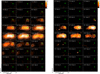 |
Fig. A.1 Channel maps of CO emission. The left (right) panel shows a channel map of 13CO (C18O) 2→1 emission from 0 to 22 (0 to 5) K km s−1 in steps of 4 km s−1 (0.3 km s−1). The green star indicates the position of the protostar. |
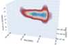 |
Fig. A.2 3D Position-velocity cut of proplyd #7 in 12CO 2→1. An interactive version is available online. |
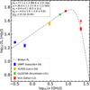 |
Fig. A.3 Radio SED of proplyd 7. The dashed line corresponds to the best fit of a broken power law (PL; see Eq. (A.1)), with the fit results given in the upper-left panel and in brackets the fit results for the same function, but excluding the first data point. The red arrow on the last data point indicates that this flux value is likely underestimated. |
Appendix B Calculation of physical properties
B.1 Column density and mass from CO data
For the calculation of the molecular gas properties such as excitation temperature, opacity, and column density (see Mangum & Shirley (2015) and Schneider et al. (2016b) for details), we assume local thermal equilibrium (LTE). In this case, the excitation temperature Tex (12CO) [K] can be derived from the main beam brightness temperature Tmb (12CO) [K], assuming this line is optically thick. This is a valid approximation because the 12CO/13CO 2→1 line ratio in proplyd #7 is typically 2–10 and thus not reflecting the interstellar 12C/13C abundance of around 60–70 (Langer & Penzias 1990, 1993; Milam et al. 2005). The excitation temperature then calculates with
![Mathematical equation: $\[\mathrm{T}_{e x}\left({ }^{12} \mathrm{CO}\right)=\frac{11.06}{\ln \left(1+11.06 /\left(\mathrm{T}_{m b}\left({ }^{12} \mathrm{CO}\right)+0.19\right)\right)}.\]$](/articles/aa/full_html/2025/12/aa57227-25/aa57227-25-eq3.png) (B.1)
(B.1)
The 13CO opacity is estimated using the excitation temperature Tex obtained from 12CO and the observed 13CO main beam brightness temperature Tmb(13CO) [K] with
![Mathematical equation: $\[\tau_{13}=-\ln \left(1-\frac{\mathrm{T}_{m b}({ }^{13} \mathrm{CO})}{\left(10.58 /(e^{10.58 / \mathrm{T}_{e x}}-1)-0.21\right)}\right).\]$](/articles/aa/full_html/2025/12/aa57227-25/aa57227-25-eq4.png) (B.2)
(B.2)
The pixel-by-pixel maps of Tex and τ13 are displayed in Fig. B.1. It becomes obvious that the excitation temperature increases from around 10 K in the outskirts of proplyd #7 to a maximum value of 35 K in the central regions. Interestingly, the peak temperatures are not found at the position of the YSO but further east. The opacity map indicates that the 13CO line is mostly optically thin with values below one across proplyd #7.
The beam averaged total column density N of the optically thin 13CO molecule can be determined from the observed line integrated main beam brightness temperature Tmb(13CO) with
![Mathematical equation: $\[N_{^{13}}{_\mathrm{CO}}=f\left(T_{e x}\right) \int \mathrm{T}_{m b}\left({ }^{13} \mathrm{CO}\right) d \mathrm{v},\]$](/articles/aa/full_html/2025/12/aa57227-25/aa57227-25-eq5.png) (B.3)
(B.3)
with
![Mathematical equation: $\[f\left(T_{e x}\right)=\frac{3 h Z}{8 \pi^3 \mu_d^2 J_u} \frac{e^{E_{u p} / k T_{e x}}}{\left[1-e^{-h \nu / k T_{e x}}\right]\left(J\left(T_{e x}\right)-J\left(T_{B G}\right)\right)},\]$](/articles/aa/full_html/2025/12/aa57227-25/aa57227-25-eq6.png) (B.4)
(B.4)
and
![Mathematical equation: $\[J\left(T_{e x}\right)=\frac{h \nu}{k\left(e^{h \nu / k T_{e x}}-1\right)},\]$](/articles/aa/full_html/2025/12/aa57227-25/aa57227-25-eq7.png) (B.5)
(B.5)
and J(TBG) = J(2.7K). h and k denote the Planck and the Boltzman constants, respectively, Eup is the energy of the upper level, ν is the frequency [GHz], μd is the dipole moment [Debye], Ju is the upper value of the rotational quantum number and ∫ Tmb(13CO) dv is the velocity integrated line intensity.
The first two terms of the rotational partition function are given by
![Mathematical equation: $\[Z=\frac{k T_{e x}}{h B}+1 / 3,\]$](/articles/aa/full_html/2025/12/aa57227-25/aa57227-25-eq8.png) (B.6)
(B.6)
with the rotational constant B expressed to first order as ν=2BJu.
For the determination of the H2 column density N(H2), we use a [12C]/13C] abundance of 70 (Langer & Penzias 1990), and a [12CO]/[H2] abundance of 8.5 10−5 (Tielens 2010). We additionally apply a correction to the hydrogen mass of a factor of 1.36 to account for helium and other heavy elements. The map of the H2 column density is displayed in Fig. B.1 and indicates typical values of molecular clouds or clumps in the range of a few 1021 cm−2 up to 2×1022 cm−2. These values correspond well to the Herschel derived column density map (Schneider et al. 2016a).
The total mass is then derived from
![Mathematical equation: $\[\mathrm{M}(_{t o t, \mathrm{CO}})=N(\mathrm{H}_2) m_{\mathrm{H}_2} ~A,\]$](/articles/aa/full_html/2025/12/aa57227-25/aa57227-25-eq9.png) (B.7)
(B.7)
with the mass of a hydrogen molecule mH2 and the area A of proplyd #7. We obtain a total mass of 16.3 M⊙ which corresponds well to the one of 19.1 M⊙ obtained from a high angular resolution (18″) map of the Cygnus region presented in Schneider et al. (2022). An earlier estimation of 47 M⊙ given in Schneider et al. (2016a) is based on a lower resolution (36″) column density map which is not corrected for fore- and background contamination (as was done in Schneider et al. 2022).
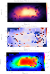 |
Fig. B.1 Maps of physical properties of proplyd #7. Top: Map of the excitation temperature derived from the 12CO 2→1 line. Middle: Map of the 13CO opacity. Bottom: Map of the H2 column density, calculated from the 13CO column density. See text for all calculations. |
From the area A, we determine an equivalent radius r of the globule with ![Mathematical equation: $\[r=\sqrt{A / \pi}\]$](/articles/aa/full_html/2025/12/aa57227-25/aa57227-25-eq10.png) and obtain r = 0.22 pc. An estimate of the density n, using the H2 column density and an extent of proplyd #7 considering a spherical geometry with n = N(H2)/(2 r), yields n = 4.4×103 cm−3.
and obtain r = 0.22 pc. An estimate of the density n, using the H2 column density and an extent of proplyd #7 considering a spherical geometry with n = N(H2)/(2 r), yields n = 4.4×103 cm−3.
B.2 Column density and mass from [C II] data
The [C II] line profiles do not show a sign of self-absorption (P Cygnus profiles with a dip at the bulk emission velocity) so that we assume the most simple scenario of a thermally excited, optically thin7 [C II] line with atomic hydrogen as the major collision partner. The [C II] column density NCII [cm−2] is then calculated (Goldsmith et al. 2012) from
![Mathematical equation: $\[N_{\mathrm{CII}}=\frac{\mathrm{I}_{\mathrm{CII}} \cdot 10^{16}}{3.43} \times\left[\left(1+0.5 \times e^{91.25 / \mathrm{T}_{k i n}}\right)\left(1+\frac{2.4 \times 10^{-6}}{C_{u l}}\right)\right],\]$](/articles/aa/full_html/2025/12/aa57227-25/aa57227-25-eq11.png) (B.8)
(B.8)
with the line integrated [C II] emission ICII in [K km s−1], the kinetic temperature Tkin [K], and the de-excitation rate Cul [s−1], which is estimated by
![Mathematical equation: $\[C_{\mathrm{ul}}=n \times R_{u l},\]$](/articles/aa/full_html/2025/12/aa57227-25/aa57227-25-eq12.png) (B.9)
(B.9)
with density n [cm−3] and de-excitation rate coefficient Rul, derived with
![Mathematical equation: $\[R_{\mathrm{ul}}=7.6 \times 10^{-10}\left(\mathrm{~T}_{k i n} / 100\right)^{0.14}.\]$](/articles/aa/full_html/2025/12/aa57227-25/aa57227-25-eq13.png) (B.10)
(B.10)
The atomic mass is then calculated via
![Mathematical equation: $\[\mathrm{M}_{(t o t, \mathrm{H})}=N(\mathrm{H}) m_{\mathrm{H}} A,\]$](/articles/aa/full_html/2025/12/aa57227-25/aa57227-25-eq14.png) (B.11)
(B.11)
with the mass mH of a hydrogen atom and assuming an [C]/[H] abundance of 1.6×10⁻⁴ (Sofia et al. 2004) for converting NCII column densities into NH column densities. We also apply the helium-contribution factor of 1.36.
There are several sources of uncertainty in these calculations. First, the value of ICII represents only a rough approximation across the region for which we have [C II] data (see Fig. 2). Second, both the kinetic temperature (Tkin) and the gas density (n) must be specified, which presents a significant challenge.
From the observed maximum main beam brightness temperature of ~9 K (Fig. 2), we obtain a Rayleigh-Jeans corrected temperature TRJ with
![Mathematical equation: $\[T_{R J}=\frac{h \nu}{k}\left[\ln \left(1+\frac{h \nu}{k T_{m b, C_{I I}}}\right)\right]^{-1}\]$](/articles/aa/full_html/2025/12/aa57227-25/aa57227-25-eq15.png) (B.12)
(B.12)
of 38 K. This is the lower limit of the excitation temperature for the [C II] line and for thermal excitation Tex ≈ Tkin. We are approximately in this limit because of the derived densities. The average density obtained from the CO data analysis is n = 4.4 × 103 cm−3 while PDR modelling yields local densities of n ~ 105 cm−3 at Position 1 (corresponding to the location of the YSO) and n ~ 104 cm−3 at Position 2 (in the more quiescent tail). In all cases, the densities are above the critical density of 3×103 cm−3 for collisions with H atoms.
We calculated the gas mass using various combinations and extreme values of these parameters. A value of M = 0.7 M⊙ is obtained for Tkin = 200 K and n = 104 cm−3, while a mass of M = 3.9 M⊙ results from Tkin = 38 K and n = 4.4 × 103 cm−3. These results suggest that the exact values of temperature and density have only a moderate influence on the derived mass. However, we emphasise once again that the [C II] intensity is based on a limited number of data points and should be regarded as an estimate. Overall, we consider the mass determination to be accurate within a factor of ~2.
B.3 Column density and mass from [O I] data
The calculation of the [O I]-column density NOI and the associated mass of the atomic gas is even more challenging to calculate than for [C II] because the line often has a high optical depth (e.g. Liseau et al. 1999; Leurini et al. 2015; Schneider et al. 2018; Goldsmith 2019) and a more complex line excitation scheme. [O I] in its ground electronic state has three fine structure levels that are inverted in energy, with the 3P0 level having the highest energy and the 3P2 the lowest. The observable fine structure transitions in the FIR are the 3P0 → 3P1 transition at 145.5 μm and the 3P1 → 3P2 one at 63.2 μm. We only have data of the 63 μm line, which can be excited by collisions with atomic hydrogen at densities above the critical density of 7.8 105 cm−3 (Goldsmith 2019). The densities in proplyd #7 are lower (maximum value is 105 cm−3 from PDR modelling), so that the excitation will be sub-thermal.
We first assume LTE conditions so that the [O I] column density is calculated (Leurini et al. 2015) with
![Mathematical equation: $\[N_{\mathrm{OI}}=\frac{8 \pi k \nu^2}{h c^3 A_{u l}} \frac{Z e^{E_j / k T_{e x}}}{g_j} \frac{\tau}{1-e^{-\tau}} \int T_{\mathrm{mb}, \mathrm{OI}} ~d \mathrm{v},\]$](/articles/aa/full_html/2025/12/aa57227-25/aa57227-25-eq16.png) (B.13)
(B.13)
with the Einstein-coefficient Aul = 8.91×10⁻⁵ s−1, c the speed of light, Ej/k = 228 K the upper level energy, gj = 3, τ the [O I] opacity, and Z the partition function that is given by
![Mathematical equation: $\[Z_{\mathrm{OI}}=\sum_{j=0}^2 g_j ~e^{-E_j / T_{e x}}=5+3 ~e^{-227.7 / T_{e x}}+e^{-326.6 / T_{e x}}\]$](/articles/aa/full_html/2025/12/aa57227-25/aa57227-25-eq17.png) (B.14)
(B.14)
The difficulty now is to to estimate the excitation temperature and the opacity. From the observed main beam brightness temperature of 2 K, we obtain a Rayleigh-Jeans corrected temperature TRJ of 48 K via Eq. B.12, adopted for [O I]. This is the lower limit for the excitation temperature and in this case, the line is subthermally excited. Typical excitation temperatures in bright and dense PDRs are higher (Leurini et al. 2015; Schneider et al. 2018), of the order of 100 to 200 K, and the [O I] 63 μm line is optically thick and shows self-absorption features (Boreiko & Betz 1996; Leurini et al. 2015; Schneider et al. 2018; Goldsmith et al. 2021). However, we do not observe self-reversal in the [O I] line profile so we assume that neither the optical depth nor the excitation temperature are very high in proplyd #7 (note that the radiation field is relatively low). Again, we calculate the [O I] column density and mass for a representative range of Tex and τ, using a [O I]/[H] abundance of 2.5×10⁻⁴ (Meyer et al. 1998) for converting NOI column densities into NH column densities. We also apply the helium-contribution factor of 1.36.
Taking a high Tex of 200 K, we obtain mass values between M = 0.04 M⊙ for τ = 1 and M = 0.13 M⊙ for τ = 5, respectively. The influence of the opacity is thus moderate. Taking the lower limit of Tex = 48 K and a marginal optically thick [O I] line (see below) with τ = 2, we get a mass of M = 1.8 M⊙. The [O I] column density in this case is then 1018 cm−2 which corresponds well to the results of optically thin or slightly optically thick, subthermally excited [O I] emission, calculated in Goldsmith (2019) using the Molpop–CEP code in a slab geometry. In their Fig. 2, an excitation temperature of 48 K corresponds to a density of ~104.5 cm−3 and a kinetic temperature Tkin of 100 K. Figure 4 gives NOI as a function of optical depth and a value of 1–5 corresponds to a NOI ~ 1018 cm−2. Figure 8 displays [O I] line profiles for Tkin = 100 K, n=104 cm−3, and a line width of 1.67 km s−1 and again, the model maximum antenna temperature of ~1.7 K for NOI = 1018 cm−2 corresponds well to our [O I] observations for proplyd #7. Interestingly, the line profile shows some indications of a flat top, but no significant dip as it is the case for higher [O I] column densities. We thus think that our observed [O I] line is only marginally optically thick with τ values of not more than a few.
In addition to the estimates given above, we applied the non-LTE code RADEX van der Tak et al. (2007) on the two positions where we performed PDR modelling, namely, position 1 with offset −4″, 0″ and position 2 with offset 36″, 0″. We calculated a parameter grid, including kinetic temperature Tkin, H2 density n(H2), and [O I]-column density NOI, in a uniform medium. Tkin was varied between 80 and 200 K, n(H2) ranged from 103 to 105 cm−3, and NOI from 0.9 × 10¹⁸ to 3 × 1018 cm−2. For all three parameters we have calculated 100 grid points. For Tkin, we used a linear spacing, and for n(H2) and NOI logarithmic spacing.
The results are not unique because we cannot unambiguously determine the densities. However, we still obtain a best-fit solution judging from the χ2. For position 1, the excitation temperature is approximately 49 K, with Tkin = 171.7 K, and n(H2) = 8.5 × 103 cm−3. For position 2, the excitation temperature is 47 K at Tkin = 171.7 K, and n(H2) = 6.4 × 103 cm−3. Both positions yield an optical depth of 1.9 and an [O I] column density of NOI = 0.9 × 1018 cm−2. All values correspond very well to what we derived from the LTE approach and by comparing to Goldsmith (2019).
In summary, the mass estimate has a larger variation depending on Tex, but considering the LTE calculations and the comparison to Goldsmith (2019), as well as the RADEX calculations, the most likely values for the [O I] column density is ~1018 cm−2 and the atomic mass is 1.8 M⊙. This value also corresponds well to the atomic mass of 1–4 M⊙ determined from the [C II] data.
All Tables
All Figures
|
Fig. 1 False-colour image of the central Cygnus X region (left; Schneider et al. 2016a) and a zoom onto the region indicated by the red dashed box around Proplyd #7 (right). The R and G channels correspond to Spitzer 8 μm, while the B channel corresponds to Herschel (PACS 70 μm) emission. The proplyd-like objects detected by Wright et al. (2012) and Schneider et al. (2016a) are labelled in yellow (pr1-11). Proplyd #7 (pr 7) is located in the upper centre region, close to some massive stars of the Cyg OB2 association. These are marked in grey, following the nomenclature in Wright et al. (2015). |
| In the text | |
|
Fig. 2 [O I] 63 μm, [C II] 158 μm, and 12CO 2→1 spectra of proplyd #7. To increase the S/N, the [O I] data were smoothed to an angular resolution of 10″ and re-gridded to 10″ (original resolution 6″ on a ~2″ sampling grid). The velocity resolution was degraded to ~0.4 km s−1. The [C II] (CO) spectra are on their nominal angular resolution of 14″ (12″) and velocity resolution of 0.2 (0.3) km s−1. The displayed main beam brightness temperature and velocity ranges are indicated in the small lower panels. The star indicates the approximate location of the YSO. |
| In the text | |
|
Fig. 3 Example of an [O I] spectrum and fit to the data. The black histogram shows the observed [O I] spectrum closest to the central YSO (position with offset −4″,0), smoothed to an angular resolution of 10″. The blue Gaussian lines represent the fit to this spectrum with two components. Centre velocity, temperature, and FWHM values are given in the panel. The red line gives the resulting fit. |
| In the text | |
|
Fig. 4 Channel map of 12CO 2→1 line emission. Each channel covers a velocity range of 0.3 km s−1. Contours go from 2 to 34 K km s−1 in steps of 4 K km s−1 and the green star indicates the position of the YSO. |
| In the text | |
|
Fig. 5 Distribution of [O I] line centre velocity and FWHM. Overlays of [O I] line integrated (v=9 to 15 km s−1) emission (contour levels 5, 6, 7, 8, and 8.5 K km s−1) on Herschel/PACS 70 μm emission in color. The left panel shows the line centre velocities in km s−1 of the two components (first component in black, second in grey) and the right panel the linewidth in km s−1. The values (Table 1) were determined from Gaussian fits to the spectra from Fig. 2. |
| In the text | |
|
Fig. 6 Spitzer 8 μm image of proplyd #7. The NIR map is in units of MJy/sr, ranging from 44 to 1.4 ± 104 with contours of [O I] emission (5, 6, 7, 8, 8.5 K km s−1) overlaid. Two positions where the PDR modelling was performed are indicated: position 1 (offset −4″,0) with a blue circle (radius 7″) and position 2 (offset 36″, 0) with a green circle, respectively. |
| In the text | |
|
Fig. 7 GLOSTAR 5.9 GHz images of proplyd #7. The top image shows the GLOSTAR data only. The image scale is in Jy/beam at an angular resolution of 4″. The star indicates the position of the YSO. The lower panel displays the same radio image with contours of 13CO 2→1 emission overlayed. The contour lines have values of 5–37.5 K km s−1 in steps of 2.5 K km s−1. |
| In the text | |
|
Fig. 8 FUV field around proplyd #7. The FUV field in Habing units (G°) is determined from the Herschel 70 and 160 μm fluxes on an angular resolution and on a grid of 11". Proplyd #7 is indicated by an arrow. |
| In the text | |
|
Fig. 9 PDR KOSMA-τ model results. The left (right) panel shows the diagnostic diagrams for UV-field and density, derived from the observed lines, line ratios, and FIR fluxes for positions 1 and 2 in proplyd #7. The red and blue dashed lines indicate the UV field determined from the FIR Herschel fluxes and from the stellar census, respectively, for positions 1 and 2. |
| In the text | |
|
Fig. A.1 Channel maps of CO emission. The left (right) panel shows a channel map of 13CO (C18O) 2→1 emission from 0 to 22 (0 to 5) K km s−1 in steps of 4 km s−1 (0.3 km s−1). The green star indicates the position of the protostar. |
| In the text | |
|
Fig. A.2 3D Position-velocity cut of proplyd #7 in 12CO 2→1. An interactive version is available online. |
| In the text | |
|
Fig. A.3 Radio SED of proplyd 7. The dashed line corresponds to the best fit of a broken power law (PL; see Eq. (A.1)), with the fit results given in the upper-left panel and in brackets the fit results for the same function, but excluding the first data point. The red arrow on the last data point indicates that this flux value is likely underestimated. |
| In the text | |
|
Fig. B.1 Maps of physical properties of proplyd #7. Top: Map of the excitation temperature derived from the 12CO 2→1 line. Middle: Map of the 13CO opacity. Bottom: Map of the H2 column density, calculated from the 13CO column density. See text for all calculations. |
| In the text | |
Current usage metrics show cumulative count of Article Views (full-text article views including HTML views, PDF and ePub downloads, according to the available data) and Abstracts Views on Vision4Press platform.
Data correspond to usage on the plateform after 2015. The current usage metrics is available 48-96 hours after online publication and is updated daily on week days.
Initial download of the metrics may take a while.