| Issue |
A&A
Volume 704, December 2025
|
|
|---|---|---|
| Article Number | A286 | |
| Number of page(s) | 13 | |
| Section | Planets, planetary systems, and small bodies | |
| DOI | https://doi.org/10.1051/0004-6361/202557330 | |
| Published online | 23 December 2025 | |
Stationary wave dynamics in Venus's upper clouds
Morphology and forcing from Akatsuki/LIR and Venus planetary climate model analyses
1
National Key Laboratory of Deep Space Exploration/School of Earth and Space Sciences, University of Science and Technology of China,
Hefei
230026,
China
2
CAS Center for Excellence in Comparative Planetology/CAS Key Laboratory of Geospace Environment/Mengcheng National Geophysical Observatory, University of Science and Technology of China,
Hefei
230026,
China
3
Laboratoire de Météorologie Dynamique (LMD/IPSL), Sorbonne Université, ENS, PSL Research University, Ecole Polytechnique, Institut Polytechnique de Paris, CNRS,
Paris,
France
4
LATMOS/IPSL, Sorbonne Université, UVSQ, Université Paris-Saclay, Centre National de la Recherche Scientifique,
Paris,
France
★ Corresponding author: This email address is being protected from spambots. You need JavaScript enabled to view it.
Received:
19
September
2025
Accepted:
17
November
2025
Abstract
Context. Stationary waves play a crucial role in vertically transporting momentum and energy in Venus’s atmosphere. Their global contributions (approximately −0.1 m s−1 day−1 at the upper cloud) are smaller than those of planetary-scale waves and meridional circulation (approximately ±1.0 m s−1 day−1), but stationary waves exert strong regional control, shaping the longitudinal structure of the super-rotating flow above highlands. Observations have linked wave signatures near the cloud top (~70 km) to underlying highland regions. However, their vertical propagation characteristics and contributions to the morphology of super-rotation remain poorly understood.
Aims. This study aims to characterize the structure, variability, and propagation of stationary waves in Venus’s atmosphere and to evaluate their role in modulating the longitudinal structure of cloud-top super-rotation.
Methods. We analyzed eight years of thermal emission data from Akatsuki/LIR to isolate stationary wave components. Simulations were performed using the high-resolution Venus planetary climate model, which incorporates a realistic topography and a hybrid vertical coordinate system.
Results. Stationary wave signatures in the brightness temperature and horizontal winds are consistently observed and simulated above highland regions, with a notable local time dependence and long-term variability. The vertical transport of angular momentum and heat dominates the wave-induced momentum and energy budget, leading to zonal wind deceleration and adiabatic heating in the upper cloud layer. Despite filtering by two weak static stability layers in the deep atmosphere, stationary waves can propagate upward and impact cloud-top dynamics.
Conclusions. Stationary waves exert a measurable influence on Venus’s upper-cloud super-rotation by vertically redistributing momentum and heat in longitude. Their effects are modulated by both vertical static stability and diurnal variations. These results highlight the crucial role of stationary waves in maintaining the observed longitudinal structure of the super-rotating atmosphere.
Key words: planets and satellites: atmospheres / planets and satellites: terrestrial planets
© The Authors 2025
 Open Access article, published by EDP Sciences, under the terms of the Creative Commons Attribution License (https://creativecommons.org/licenses/by/4.0), which permits unrestricted use, distribution, and reproduction in any medium, provided the original work is properly cited.
This article is published in open access under the Subscribe to Open model. This email address is being protected from spambots. You need JavaScript enabled to view it. to support open access publication.
1 Introduction
The Venusian atmosphere exhibits a rapid westward zonal flow, known as super-rotation, which reaches velocities exceeding ~100 m/s near the cloud tops at ~70 km, approximately 5060 times faster than the rotation of the solid surface (Read & Lebonnois 2018). Despite extensive observational and modeling efforts aimed at elucidating the mechanisms that sustain and modulate this super-rotation (Fukuya et al. 2021 ; Lai et al. 2024; Lebonnois et al. 2010; Takagi et al. 2023), its longitudinal structure and the underlying forcing processes remain poorly constrained. Of the proposed mechanisms, stationary waves capable of transporting momentum and energy both vertically and horizontally have emerged as key factors that potentially influence the longitudinal variability of the atmospheric flow. However, the detailed dynamics governing the propagation of these waves and their role in shaping the super-rotation are yet to be fully understood.
The first topography-related stationary waves on Venus were detected by the Vega balloons, which observed enhanced vertical wind, temperature, and pressure perturbations around 53 km over elevated terrain (Blamont et al. 1986; Sagdeev et al. 1986). More recently, a large stationary wave with a bow-shaped structure extending over 10 000 km in latitude was observed at ~65 km altitude above highland regions by the Longwave Infrared Camera (LIR) on board Akatsuki (Fukuhara et al. 2017a). Complementary statistical detections of mountain-related stationary waves have been reported using data from the Venus Infrared Thermal Imaging Spectrometer (VIRTIS; Peralta et al. 2017), the Venus Monitoring Camera (VMC; Piccialli et al. 2014), and the Radio Science Experiment (VeRa; Tellmann et al. 2012) on board Venus Express. Recent VIRTIS-M dayside observations have consistently shown similar wave properties in the lower and upper clouds, but no direct correspondence between them in shape or relative position (Silva et al. 2024). These studies reveal a clear interaction between the upper clouds and surface topography but little correlation with the lower clouds. This complex behavior likely arises from the interplay of topographic forcing, convective processes, and Kelvin-Helmholtz instabilities within the context of Venus’s deep atmosphere, which is characterized by two weakly stable layers at altitudes of 18-30 km and 48-55 km (Lebonnois & Schubert 2017; Tellmann et al. 2012).
Mesoscale modeling nested within lower-resolution general circulation models (GCMs) suggests that mountain waves can propagate through the two weakly stable layers in the deep atmosphere. However, much of their energy is deposited into these regions (Lefèvre et al. 2020). Contrastingly, at high latitudes, thicker mixed layers in the deep atmosphere appear to suppress wave activity at cloud-top levels in simulations, contradicting VeRa observations that show concentrated wave activity in upper clouds at these latitudes (Tellmann et al. 2012). Furthermore, sub-grid-scale orographic parameterizations in the Venus planetary climate model (PCM) produce stationary mountain waves at altitudes of around 35 km that remain detectable in high-latitude upper clouds, suggesting that convective layers do not entirely block such waves (Navarro et al. 2018). Consequently, elucidating the mechanisms of stationary wave propagation through Venus’s deep atmosphere is critical for understanding their impact on the upper cloud dynamics.
In addition, time-averaged background zonal winds from UV observations show significantly reduced velocities - by approximately 20 m/s - above the Aphrodite Terra highland compared to those above flatter regions (Bertaux et al. 2016). This zonal wind deceleration is also modulated by local time (Patsaeva et al. 2019) and the long-term variability of superrotation (Patsaeva et al. 2024), complicating the relationship between surface topography and cloud-top circulation. A highresolution T63 (triangular spectral truncation with a maximum wavenumber of 63) Atmosphere and Ocean Research Institute (AORI) Venus GCM employing sigma coordinates has been used to investigate the stationary components of the atmospheric field, revealing enhanced wave activity in the cloud tops above high-latitude highland regions (Yamamoto et al. 2021). Notably, while planetary-scale waves such as thermal tides and Rossby and Kelvin waves dominate the global momentum and energy balance (Lai et al. 2025; Yamamoto et al. 2023, 2024), these regionally confined stationary waves exert strong control over the longitudinal variability of the super-rotating flow (Bertaux et al. 2016; Yamamoto et al. 2021).
Stationary wave characteristics vary considerably across GCMs, underscoring the need for model intercomparisons to identify robust features. The Venus PCM, which incorporates realistic topography and a hybrid vertical coordinate system, has been validated against mesoscale model results, while T63-resolution GCMs have been shown to capture stationary wave patterns. In this study, we used a higher-resolution version of the Venus PCM (around T95) and combined its output with Akatsuki/LIR observations to conduct a comparative analysis based on temporally averaged fields. Such averaging is a practical approach for isolating stationary components and evaluating their typical characteristics as well as their contributions to the maintenance and longitudinal structure of super-rotation.
2 Datasets and methods
2.1 Akatsuki/LIR observations and analysis
Akatsuki/LIR is a broadband mid-infrared imager operating in the 8-12 μm range, capable of detecting thermal emission from both the dayside and nightside of the Venusian atmosphere. Image acquisition typically occurs every 1-2 hours along Akatsuki’s elongated equatorial orbit, which has a period of ~11 days, with an apoapsis of ~360 000 km (~300 km resolution) and a periapsis of 1000-8000 km (~7 km resolution; Nakamura et al. 2016). The LIR primarily senses thermal emission from the 65±10 km altitude level, according to its contribution function (Taguchi et al. 2007). The relative uncertainty is ~0.3 K for a nominal brightness temperature of 230 K, and the absolute accuracy is within 3 K (Fukuhara et al. 2011). However, recent assessments suggest that LIR underestimates infrared radiance by ~ 15-17% (Nishiyama et al. 2025), requiring caution in interpreting absolute brightness temperatures. In this study, we used Level 3d mapped brightness temperature data (Murakami et al. 2018), which were calibrated using the baffle (hood) temperature (Fukuhara et al. 2017b) and correlated to account for detector sensitivity degradation (Taguchi et al. 2023). To ensure data quality and consistency with the model resolution, we used only images acquired between October 2016 and December 2023, excluding periods affected by power supply fluctuations (Fukuhara et al. 2017b). Furthermore, observations taken at orbital altitudes exceeding 150 000 km are excluded to maintain a comparable horizontal resolution (~130 km, equivalent to 1.25° longitude at the equator) with the Venus PCM simulations used in this study.
The original Level 3d maps are first re-gridded onto a 288 × 144 longitude-latitude grid. The limb-darkening effect, caused by the increase in effective sensing altitude with emission angle (Akiba et al. 2021; Longobardo et al. 2012), is then corrected using the method described in Lai & Li (2023). Specifically, the brightness temperature (T) is fitted as a function of the cosine of the emission angle (θ) using the relation
 (1)
(1)
where T0 is the nadir brightness temperature, and C is a fitted constant value. The brightness temperature in each image is then scaled to its T0. The cloud motions are derived using the cloud tracking method in Fukuya et al. (2021), adopting the same settings as in Lai & Li (2023), but with improved treatment of the longitudinal boundary by explicitly accounting for the periodicity in longitude during high-pass filtering and template matching. This correction effectively eliminates artificial discontinuities in horizontal winds near the longitudinal boundary 0°/360°.
To extract stationary features from highly variable meteorological data, temporal averaging is applied in geographic coordinates. A suitable time window for averaging is defined by constructing a Venus date index through fitting a sawtooth function to the subsolar longitude, based on local time variations derived from LIR observations (Fig. 1). Observations are binned into 2-Venus-hour intervals (Figs. 1b-d), followed by a 5-Venus-day running mean with Gaussian weighting in time. The long-term decay of brightness temperature observed here is consistent with that from Earth-orbiting satellites (Nishiyama et al. 2025). This may reflect the influence of solar activity cycles, as suggested by previous analyses (Khatuntsev et al. 2022). Venus PCM simulations indicate that both the zonal wind and temperature respond approximately in proportion to variations in the solar heating rate (Lee et al. 2019). However, recent observations after early 2021 do not show a clear correlation with solar cycle variations (Horinouchi et al. 2024). Given that the current continuous record spans only about 16 years -less than two solar cycles - it remains uncertain whether this long-term variation is caused by solar activity or other dynamical or radiative processes. Furthermore, contrasting variation trends between equatorial and midlatitude regions indicate oscillations in the meridional circulation, whose horizontal angular momentum (AM) flux impacts the equatorial and midlatitude jets responsible for cloud super-rotation (Lai et al. 2024).
Temporal averaging intends to suppress thermal tides; however, due to uneven temporal distribution of observations, atmospheric thermal tidal signals persist and must be removed. To remove thermal tides, the 2-Venus-hour binned data (shown as scattered points in Figs. 1b-d) are transformed from geographic to solar-fixed coordinates. In this frame, a Gaussian-weighted 5-Venus-day running mean is applied, and thermal tides are extracted via least-squares harmonic fitting using local time wavenumbers 1-4. According to previous studies on thermal tides (Kouyama et al. 2019; Zasova et al. 2002), wavenumbers 1-4 are the main components in the Venus middle-to-lower atmosphere. We also tested higher wavenumbers (1-8), but their inclusion did not alter the results. The fitted tidal components are then subtracted from each 2-Venus-hour mean field. Finally, median values of the thermal-tide-corrected data are computed at each spatial grid point to reduce the impact of outliers and robustly isolate stationary components of brightness temperature and horizontal winds (Fig. 2).
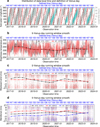 |
Fig. 1 Distribution and smoothing of Akatsuki/LIR data. Panel a : distribution of brightness temperature (gray dots) and derived cloud-tracked winds (cyan dots) as a function of local time and observation date. Black dots indicate the subsolar longitude of each image. The defined Venus date was derived by fitting a sawtooth function to the subsolar longitude. Panels b-d: 1/12 Venus-day means of brightness temperature (b), zonal wind (c), and meridional wind (d). The solid lines represent 5-Venus-day running means applied to each variable. |
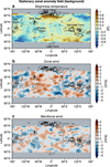 |
Fig. 2 Zonal anomalies of stationary features observed by Akat-suki/LIR. Panels show brightness the temperature (a), zonal wind (b), and meridional wind (c) after a temporal median is applied following thermal tide removal. Color shading indicates zonal anomalies relative to the longitudinal mean at each latitude. Black contours indicate the surface topography at elevations of 1, 3, and 5 km, with major highland regions labeled in panel a. Gray areas indicate regions with insufficient valid data. For the wind (brightness temperature) data, areas left with fewer than 20 (40) valid measurements after the removal of thermal tides are left empty (see Fig. A.1a). |
2.2 Venus PCM simulations
The Venus PCM is based on the Laboratoire de Météorologie Dynamique zoom model, which employs a finite-difference dynamical core in latitude-longitude coordinates (Hourdin et al. 2006). It includes a comprehensive radiative transfer scheme (Lebonnois et al. 2010) using precomputed solar heating tables based on latitudinally varying cloud distributions (Haus et al. 2014, 2015), a soil model (Hourdin et al. 1993), and a topographic boundary layer scheme (Lebonnois et al. 2018). The analyzed simulation, described in detail by Lai et al. (2024, 2025), uses output from the final 5 Venus days.
The model is configured with a horizontal resolution of 288 longitudes × 144 latitudes and 50 vertical levels, using hybrid vertical coordinates extending from the surface up to ~95 km. The hybrid vertical coordinate is defined as p = αp + bppsurf (see Table 1 of Lebonnois et al. 2010), where bp scales the influence of surface pressure (psurf ) on the vertical levels. Larger bp values enhance stationary-wave amplitudes near the surface, at levels, but above ~20 km in this simulation, bp is small (<0.1), so the hybrid coordinate has minimal impact on wave propagation at upper levels. Temporally averaged stationary features, 〈X〉, of various model variables (X) are shown in Fig. 5. The Scorer parameter (l), which characterizes the minimum vertical wavelength for gravity wave propagation (Lefèvre et al. 2020; Scorer 1949), was computed as
 (2)
(2)
where N is the Brunt-Väisälä frequency, u is the zonal wind, and z is the altitude. This parameter l indicates the vertical propagation conditions of stationary (Lee) waves. If l2 remains nearly constant with height, internal gravity waves generated by mountains propagate vertically and do not change to external ones. If l2 decreases rapidly with altitude, waves with horizontal wavenumber, k > l, can become trapped below that level (trapped Lee waves). Conversely, if l2 increases with height, vertical wave propagation is generally suppressed. The Richardson number (Ri), a nondimensional measure of the ratio of static stability to vertical shear of horizontal winds (Miles 1961), is defined as
 (3)
(3)
where v is the meridional wind. Values of Ri < 0.25 indicate conditions favorable for the development of Kelvin-Helmholtz instabilities, where vertical shear dominates stratification and can lead to wave dissipation. Conversely, regions with Ri > 1 are generally considered stable for wave propagation.
3 LIR-observed stationary features
To evaluate the background horizontal stationary features, zonal anomalies of brightness temperature, zonal wind, and meridional wind are examined (Fig. 2), based on the methodology described in Sect. 2, with thermal tides removed. To ensure the robustness of the final stationary structure, we followed a similar approach to that of Fukuya et al. (2021), retaining only spatial grids with enough valid data points (Fig. A.1a). In addition, we verified the results using the longitudinal gradient of brightness temperature to fit and remove thermal tides, ensuring that the anomalies in each image were not affected by absolute values from different observation times. The resulting stationary structures remained nearly identical, confirming that the outcome is not influenced by the thermal tide removal. The brightness temperature generally exhibits higher values above highland regions in the upper cloud layer, especially in the midlatitudes (see Fig. A.1c). At higher latitudes, the correlation remains unclear due to limited data coverage. Nonetheless, planetary-scale stationary waves with wavenumbers 2-4 may be present, as suggested by previous GCM simulations (Yamamoto et al. 2021).
Instantaneous LIR images often show large-scale bowshaped stationary waves associated with enhanced brightness temperatures (Fukuhara et al. 2017a; Kouyama et al. 2017), supporting the validity of the features extracted here. For zonal wind (defined as positive westward in this study), reduced flow speeds are observed over highland regions at cloud-top levels (Fig. 2b), consistent with VMC-derived dayside wind fields (Bertaux et al. 2016). Since LIR senses slightly lower altitudes (~65 km) than VMC (~70 km), this may indicate the vertical propagation and dissipation of stationary waves within the upper cloud layer. However, the ~30° longitudinal offset between zonal wind minima and topography reported in VMC observations is not evident in the LIR data. This discrepancy may result from local time dependence (Patsaeva et al. 2019) and temporal variability of the stationary structures (Patsaeva et al. 2024).
For meridional wind, although some topographic correlations have been reported in VMC data, no significant relationship is apparent in the LIR results (Fig. 2c). This may be due to LIR’s lower sensitivity to meridional motions or intrinsically weaker topographic coupling in the meridional wind field (Bertaux et al. 2016; Patsaeva et al. 2019).
The generation of stationary waves is favored in the afternoon sector due to the diurnal cycle of near-surface atmospheric stability, which becomes more conducive to wave excitation during this period (Navarro et al. 2018). Statistical analyses of LIR observations further indicate that large-scale stationary waves are more frequently detected from noon to afternoon (Kouyama et al. 2017). This preference may contribute to a westward shift of the dayside zonal wind stationary features by approximately 90°, spanning from 10 to 16 local time at cloud-top altitudes (Patsaeva et al. 2019).
Because LIR senses thermal emissions from both the dayside and nightside upper clouds, it enables a more comprehensive analysis of the diurnal dependence of stationary wave structures. As shown in Fig. 3, brightness temperature and horizontal winds averaged over the 5°S-15°S latitude band exhibit pronounced local time-dependent variations. The westward shift of the stationary brightness temperature pattern is particularly evident, progressing at a rate of ~15-20° per Venus hour, consistent with the ~15°Zhour shift previously reported by VMC for dayside features.
A similar westward progression is apparent in the LIR-derived zonal wind field, though less pronounced, likely due to the limited availability of reliable cloud-tracked wind vectors. This shift occurs between 10 and 16 local time, with a localized disturbance near 13 hours that may be due to data quality issues. Although the meridional wind shows no clear correlation with surface topography, it also exhibits a westward displacement. Mesoscale model simulations suggest that the vertical gradient of static stability varies with local time, being strongest near midnight and weakest in the afternoon close to the surface. This diurnal variation favors the upward propagation of gravity waves with shorter vertical wavelengths around noon and in the afternoon (Lefèvre et al. 2020). Consequently, enhanced vertical wave propagation is expected during these hours, consistent with the elevated brightness temperatures observed over Aphrodite Terra in the afternoon sector (Fig. 3b).
Long-term analyses combining dayside cloud-top winds from Venus Express/VMC and Akatsuki UV imager have revealed that the zonal wind exhibits distinct longitudinal responses to variations in the background circulation, with larger amplitude fluctuations observed above highland regions such as Aphrodite Terra (Patsaeva et al. 2024). Fig. 4 presents corresponding results from LIR at a slightly lower altitude (~65 km), following the removal of diurnal cycle variations.
At low latitudes, the background zonal wind shows a decreasing trend from Venus day 149 to 157, followed by an increase through day 161 (Fig. 1c). Its temporal evolution coincides with a reduced contrast in both the brightness temperature and the zonal wind between Aphrodite Terra and surrounding lowland regions during Venus days 151-158 (Figs. 4a and 4b). Interestingly, this behavior is consistent with previous findings at cloud-top levels on the dayside. The observation of similar features by different instruments at different altitudes suggests that this is a robust phenomenon, although its underlying mechanism remains unclear. To date, no comprehensive explanation has been proposed. Capturing this behavior likely requires simulations that incorporate time-dependent solar forcing.
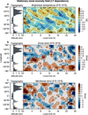 |
Fig. 3 Local time dependence of zonal anomalies near Aphrodite Terra (5°S-15°S). Panels show brightness temperatures (a), zonal winds (b), and meridional winds (c) based on observations binned into 2-Venus-hour intervals in defined Venus Universal Time (Venus UT). The resulting fields are projected onto local time-longitude coordinates, and the median value is taken in each bin over the 5°S-15°S latitude band. Color shading indicates deviations from the zonal mean at each local time. |
4 Stationary waves and their propagation simulated by the Venus PCM
Although mesoscale models have been employed to investigate stationary mountain waves over specific highland regions (Lefèvre et al. 2020), high-resolution GCMs remain essential for characterizing the global influence of stationary waves on the horizontal structure of Venus’s cloud layers (Yamamoto et al. 2021). The Venus PCM incorporates surface topography, slope wind effects (Lebonnois et al. 2018), and a hybrid vertical coordinate system, making it suitable for simulating vertically propagating stationary waves.
Fig. 5 presents the temporally averaged stationary wave structures at three altitude levels - 30 km (deep atmosphere), 50 km (lower clouds), and 70 km (cloud top) - in terms of temperature, vertical velocity, and horizontal winds. At ~30 km, near the upper boundary of the deep mixed layer, clear stationary wave signatures are visible: temperature decreases, zonal winds weaken, and vertical wind amplitudes increase over highland regions. In contrast, meridional winds do not show consistent correlations with topography at any level and are thus not discussed further.
At ~50 km, near the base of the convective layer (48-55 km), the influence of surface topography weakens, except in high-latitude mountainous regions. This attenuation is likely due to the partial filtering of stationary waves by the two low-stability layers in the deep atmosphere, as discussed later in Fig. 7.
At cloud-top level (~70 km), large-scale stationary wave patterns reappear with temperature maxima (~0.2-0.4 K) over highland terrain (Figs. 5a, 6a), similar to Akatsuki/LIR observations above Alta Regio, Aphrodite Terra, and the Phoebe Regio (Fig. 6b). Enhanced mesoscale disturbances over highlands (~0.2 K) are likewise consistent with LIR results (Figs. 6c-f).
Vertical velocity, being directly linked to vertical wave propagation, serves as a sensitive tracer of stationary wave activity and reveals coherent structures extending from the surface to the cloud top. Zonal winds are reduced (~1 m/s) above highland regions, in agreement with AORI GCM simulations (~2 m/s; Yamamoto et al. 2021) and LIR observations (~2-3 m/s). These values are substantially lower than those derived from dayside UV observations (~20 m/s), likely reflecting strong local time dependence in the manifestation of stationary wave features (Fig. 3; see also Kouyama et al. 2017; Patsaeva et al. 2019).
At high latitudes, vertically propagating stationary waves are more prominent, exhibiting a planetary-scale structure with zonal wavenumber 2. These features closely resemble those produced by the AORI Venus GCM. They are consistent with Akatsuki/LIR observations, supporting the robustness of the stationary wave patterns generated by the Venus PCM’s boundarylayer scheme. However, mesoscale simulations indicate that most mountain waves are filtered out at high latitudes due to the presence of a thicker low-stability layer (Lefèvre et al. 2020), underscoring the need for future high-resolution GCMs to resolve this discrepancy.
To investigate the vertical propagation of stationary waves, Fig. 7 shows vertical cross sections across low-latitude (Aphrodite Terra, 10°S) and high-latitude (Ishtar Terra, 65°N) mountainous regions. The vertical structure of the stationary vertical wind exhibits enhanced amplitudes within the lower mixed layer and immediately above the highland surfaces. In both regions, wave propagation is strongly attenuated between the two weakly stable layers, where most wave energy is filtered. Nevertheless, above the highlands, a portion of the wave signal persists beyond ~50 km, with reduced amplitudes and reversed horizontal phase tilts, and shows renewed growth with altitude in the clouds.
In the weakly stable layers (Fig. B.1), the Scorer parameter (see Sect. 2) becomes small or even negative, thereby inhibiting vertical wave propagation. Vertical flows are amplified below ~40 km but weaken sharply around this altitude (Figs. 7a, b). This sudden weakening is unlikely to be caused by the hybrid coordinate, since bp is already small above 20 km. Rather, it results from a rapid increase in static stability, which raises the Scorer parameter and suppresses vertical propagation of gravity waves (Figs. B.1a, 7c and 7d). Similar behavior is seen in mesoscale simulations (see Fig. 6 of Lefèvre et al. 2020) and the AORI Venus GCM with non-hybrid coordinates (see Fig. 7b of Yamamoto et al. 2021). While the hybrid coordinate can slightly modulate stationary-wave amplitudes, the dominant factor for the weakening around 40 km is the vertical variation of static stability. Consequently, only a fraction of the stationary wave energy can penetrate these layers. According to estimates by Lefèvre et al. (2020) using the method of Sutherland & Yewchuk (2004), the first barrier (18-35 km) can attenuate approximately 79% of wave energy, and the second (48-54 km), around 16% at low latitudes. At high latitudes, the second barrier alone can account for a reduction of ~55% in wave energy.
Despite this stronger filtering at high latitudes - due to a thicker convective layer - the initial wave amplitudes are significantly larger in these regions, with vertical wind perturbations approximately three times greater than at low latitudes. This implies that wave energy is nearly an order of magnitude higher at high latitudes, allowing stationary waves to remain prominent even after partial attenuation. These results support the idea that high-latitude stationary wave activity remains dynamically significant despite strong filtering. Akatsuki/LIR observations are mostly limited to midlatitudes, and additional high-latitude measurements are needed to confirm this behavior. Nevertheless, statistical analyses from radio occultation and infrared imagery indicate enhanced gravity wave activity at high latitudes (Mori et al. 2021; Silva et al. 2021; Tellmann et al. 2012). Similarly, simulations with the AORI GCM also show stronger stationary wave propagation at high latitudes (Yamamoto et al. 2021).
Eliassen-Palm (EP) flux, F = (0, F(φ), F(z)), is a traditional diagnostic tool used to characterize wave-induced AM transport in the atmosphere, particularly in the latitude-altitude plane (Fig. 8a). It is defined following Andrews et al. (1987) as
![Mathematical equation: \begin{cases} F^{(\phi)} = \rho_0 a \cos\phi \left( \bar{u}_z \frac{\overline{v'\theta'}}{\bar{\theta}_z} - \overline{v'u'}\right), \\[1ex] F^{(z)} = \rho_0 a \cos\phi \left\{ \left[f - \frac{1}{a\cos\phi}\frac{\partial}{\partial \phi}(\bar{u}\cos\phi)\right] \frac{\overline{v'\theta'}}{\bar{\theta}_z} - \overline{w'u'} \right\}. \end{cases}](/articles/aa/full_html/2025/12/aa57330-25/aa57330-25-eq4.png) (4)
(4)
Here, overbars denote zonal means, primes denote zonal anomalies, and the variables σ0, a, θ, w represent basic air density, planetary radius, potential temperature, and vertical wind, respectively. In the context of stationary waves, each variable (X) is first temporally averaged over the 5 Venus days, denoted (X). The vertical AM flux (〈w〉′〈u〉)′ cos φ, as shown in Fig. 7c) is equal to  times the vertical AM flux term of EP flux (Fig. 8b). The zonal acceleration associated with EP flux divergence is computed as
  from the transformed Eulerian-mean (TEM) momentum equation. Caution is needed when applying the TEM equations in low-stability layers, particularly around 30 km altitude, because θz approaches zero, which can lead to an unphysical amplification of the EP flux (see Fig. B.1). From the TEM thermodynamic equation, the wave-induced adiabatic heating can be estimated as
![Mathematical equation: \bar{\theta}_t \approx -\frac{1}{\rho_0} \left[ \rho_0 \left(\frac{\overline{v'\theta'}}{a}\frac{\bar{\theta}_\phi}{\bar{\theta}_z}+\overline{w'\theta'} \right)\right]_z \,,](/articles/aa/full_html/2025/12/aa57330-25/aa57330-25-eq7.png) (5)
(5)
The vertical heat flux term associated with stationary waves is represented by  .
.
Vertical AM fluxes are enhanced above highland regions at both low and high latitudes (Figs. 7e, f), exerting a measurable influence on the zonal structure of the upper cloud layers. Notably, the flux is predominantly negative in these areas, indicating upward transport of westward momentum. This contributes to a deceleration of zonal winds above mountainous regions at cloud-top altitudes, as shown in Fig. 8b. As expected for stationary waves, the vertical component dominates the EP flux. This deceleration is consistent with LIR in Sect. 3 and UV observations (Bertaux et al. 2016; Patsaeva et al. 2019, 2024), which report weakened wind speeds over highlands at cloud-top levels, suggesting that stationary waves dissipate near the cloud top. To explain the ~20 m/s zonal wind reduction observed on the dayside above mountainous regions by VMC (Bertaux et al. 2016), a deceleration rate of approximately −0.1 m s−1 day−1 would be required - an order of magnitude larger than that simulated by the Venus PCM. However, LIR observations indicate zonal wind reductions roughly one order of magnitude smaller than those inferred from VMC, and even mesoscale simulations with horizontal resolutions of 15-40 km yield deceleration rates about four times smaller than those required. Although the precise contribution of stationary waves to the observed wind deceleration remains uncertain, both modeling and observations suggest that they constitute one of the primary mechanisms responsible for slowing the zonal winds at upper cloud above Venusian highlands.
Between 40 and 45 km, both EP and AM fluxes are notably weakened in low to midlatitudes, likely due to the strong filtering effect of the low-stability layer between 18 and 35 km. In contrast, this effect is less pronounced at high northern latitudes, possibly because of the steep topographic gradients of Ishtar Terra (Yamamoto et al. 2021). Such filtering suppresses the upward propagation of AM fluxes above relatively flat regions, consistent with the trapping effect associated with a low Scorer parameter (Lefèvre et al. 2020). The extremely high EP fluxes between 30 and 40 km at ~60°N/S may arise from unphysical amplification caused by small vertical gradients of potential temperature (Fig. B.1b). The alternating directions of vertical AM fluxes below 40 km likely reflect the superposition of zonal-mean signals over regions with varying stability, influenced by convective activity and local instabilities. As shown in Fig. 9b, stationary waves generally propagate upward below 40 km above the mountain regions.
The enhanced temperatures observed above highland regions at upper cloud levels can be partly attributed to adiabatic heating induced by stationary waves. In these layers, net heating exhibits a vertically layered pattern of alternating warming and cooling, with the vertical heat flux component playing a dominant role (Figs. 8c, d). Around the LIR-sensitive altitude (~65 km), and particularly above 70 km, net heating becomes more pronounced and shows a clear spatial correlation with surface topography in the midlatitudes. At high latitudes, by contrast, topography-related heating signals are less evident. This may result from the presence of planetary-scale stationary waves, whose dynamics remain poorly understood (Figs. 5 and 6; see also Yamamoto et al. 2021), and which may mask localized heating signatures associated with topography. In the deep atmosphere, the strongly neutral stratification between ~18 and 35 km appears to trap and dissipate a significant portion of the stationary wave energy. This trapping leads to localized energy and momentum deposition near the surface, as indicated by vertical profiles of adiabatic heating and acceleration rates, both of which show strong coupling to the underlying topography at these altitudes.
To examine the local time dependence of stationary waves, Venus PCM outputs are transformed into a local time framework at each longitude and latitude. Fig. 9 illustrates results over the Aphrodite Terra latitude band. Notably, low zonal wind speeds are more clearly associated with Alta Regio (120°W-180°W) during the dayside, in agreement with LIR observations. In contrast, over Aphrodite Terra, the cloud-top zonal wind unexpectedly exhibits higher velocities on the dayside. This may reflect weaker coupling between the surface topography of Aphrodite Terra and the overlying cloud-top flow, compared to Alta Regio (see Figs. 5, 6, and 7). The underlying mechanism remains unclear but may be related to the double-peaked longitudinal structure of Aphrodite Terra, which could induce more complex stationary wave patterns than those generated by isolated mountains (Smith 1979). Similar signatures of weaker mountain waves over Aphrodite Terra have also been reported in mesoscale simulations (Lefèvre et al. 2020) and the AORI GCM (Yamamoto et al. 2021).
The longitudinal structure in the Venus PCM shows a westward drift with increasing local time, with a phase speed of approximately 15° per Venus hour - comparable to that observed in both LIR and VMC datasets (~15-20° per Venus hour on the dayside). This local time dependence is primarily governed by vertical propagation conditions for stationary waves, as represented by the Ri number in Fig. 9b. In contrast, the Scorer parameter shows little sensitivity to local time, indicating a limited role in modulating diurnal wave behavior.
Within the 40-60 km altitude range, Ri exhibits strong local time variability that closely follows changes in the vertical AM flux (Fig. 9c). Between 9 and 17 Venus hours, near the second topographic peak of Aphrodite Terra (noting the westward background flow), Ri low values (<0.25) extend over a broader altitude range from the surface, while intermediate values (5-10) occur at lower altitudes, implying enhanced wave dissipation and momentum deposition in the deep atmosphere. This leads to reduced upward propagation and results in weaker deceleration - or even acceleration - of the cloud-top zonal wind, consistent with observed higher wind speeds. At other local times, higher Ri values favor wave propagation and the associated deceleration at the cloud top.
A comprehensive understanding of the long-term variability, such as the 12-year cycles reported by Patsaeva et al. (2024), and its impact on stationary waves will require model developments capable of capturing realistic fluctuations in the background wind field, which is beyond the scope of this study.
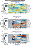 |
Fig. 4 Temporal variations of zonal anomalies near Aphrodite Terra (5°S-15°S). A 5-Venus-day Gaussian smoothing is applied along the Venus date axis, followed by thermal tide removal via harmonic fitting at each smoothed field within the 5°S-15°S latitude band. Panel a : brightness temperatures. Panel b : zonal winds. Panel c : meridional winds. Color shading indicates deviations from the zonal mean. The red rectangles indicate the regions where the longitudinal contrasts are reduced over time. Gray areas indicate regions without data. |
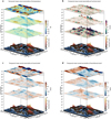 |
Fig. 5 Horizontal structure of stationary waves simulated by the Venus PCM, averaged over 5 Venus days. Panels show air temperatures (a), vertical winds (b), zonal winds (c), and meridional winds (d) at three altitude levels: deep atmosphere (−30 km), lower clouds (~50 km), and cloud top (~70 km). Black contours indicate the underlying surface topography, with elevations corresponding to major highland regions. Undulations on each horizontal slice represent the absolute values of anomalies scaled by two standard deviations (〈X〉′/2σ) to enhance visibility in the 3D perspective. |
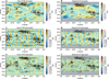 |
Fig. 6 Comparison of horizontal stationary features at the cloud top between the Venus PCM (a, c, and e) and Akatsuki/LIR (b, d, and f), analogous to Figs. 2 and 5 but decomposed using longitudinal filters: low-pass (a and b; wavenumber ≤6), band-pass (c and d; 6 ≤ wavenumber ≤12), and high-pass (e and f; wavenumber ≥12). |
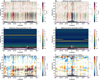 |
Fig. 7 Vertical structure of stationary waves at latitudes corresponding to Aphrodite Terra (a, c, and e; 10°S) and Ishtar Terra (b, d, and f; 65°N) in the Venus PCM, averaged over 5 Venus days. Panels a and b: zonal anomalies of vertical wind (color shading), overlaid with streamlines of vertical and zonal wind. The vertical wind is normalized at each altitude level for visibility. Panels c and d: scorer parameter. Panels e and f : vertical AM flux associated with stationary waves, calculated as 〈w〉′〈u〉′ cos φ. |
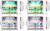 |
Fig. 8 AM transport (a and b) and adiabatic heating (c and d) associated with stationary waves in the Venus PCM. Panels a and b: EP flux and the vertical flux of AM (arrows; both divided by basic air density), along with the corresponding zonal wind acceleration (color shading). Panels c and d: Adiabatic heating induced by stationary waves and the associated vertical heat flux component. Light and dark gray shading indicates, respectively, the maximum and mean surface topography at each latitude. Black contours represent the background zonal wind (m/s). |
5 Conclusions
We investigated the characteristics and vertical propagation of stationary waves in the Venusian atmosphere using long-term Akatsuki/LIR observational data and simulations from the Venus PCM. Stationary wave features in the brightness temperature and upper-cloud winds were extracted from LIR data, and this revealed clear longitudinal anomalies aligned with highland regions. These anomalies exhibit a strong local time dependence and long-term variations that are correlated with the background wind. The results are broadly consistent with previous cloud-top observations and confirm vertical propagation at the slightly lower altitudes detectable by LIR.
The simulations reproduce the observed stationary wave patterns, including enhanced vertical wind amplitudes, temperature perturbations, and reduced zonal wind speeds above highlands. These features display coherent vertical structures extending from the deep atmosphere to the cloud tops. The model captures the filtering effects of two low-static-stability layers in the deep atmosphere, consistent with theoretical predictions and mesoscale studies. Simulated zonal wind deceleration and EP flux divergence confirm that stationary waves contribute significantly to AM redistribution and modulate the super-rotating flow in longitude. Vertical AM flux dominates wave-induced momentum transport. Simulated adiabatic heating suggests that vertical heat transport by stationary waves affects the thermal structure, particularly near 65 km. At high latitudes, however, the heating patterns are more complex and less clearly associated with topography, likely due to the influence of planetary-scale stationary waves, which are not yet fully understood.
These findings highlight the important role of stationary waves in shaping the longitudinal and temporal variability of the Venusian atmosphere, particularly in the cloud-top region for which observational constraints exist. The agreement between observations and model results demonstrates the Venus PCM’s ability to represent key dynamical processes. Future progress will require higher model resolution and extended observational coverage, especially at high latitudes and over longer timescales, to fully understand the life cycle of stationary waves and their role in maintaining super-rotation.
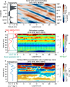 |
Fig. 9 Local time dependence of zonal anomalies near Aphrodite Terra (5°S-15°S) in the Venus PCM. Panel a : brightness temperature. Panel b: Richardson number and vertical propagation of stationary waves (arrows; −ρ0a〈w〉′〈u〉′ cos φ). Panel c: zonal acceleration induced by stationary waves expressed as |

Acknowledgements
The work described in this paper was carried out at the University of Science and Technology of China, with support from the National Natural Science Foundation of China Grant 42130203. This study benefited from the IPSL Data and Computing Center ESPRI, which is supported by CNRS, Sorbonne Université, CNES and Ecole Polytechnique, as well as from the High-Performance Computing (HPC) resources of the HPC resources of Centre Informatique National de l’Enseignement Supérieur (CINES) under the allocation n° A0120110391 made by Grand Equipement National de Calcul Intensif (GENCI). D.L. was supported by the National Natural Science Foundation of China (42508018) and the Fundamental Research Funds for the Central Universities (WK2080250235). M.L. acknowledges receiving funding from the European Union’s Horizon Europe research and innovation program under the Marie Sklodowska-Curie grant agreement 101110489/MuSICA-V. The Akatsuki project of JAXA provided the data used in this study. We thank all the members of the Akatsuki Mission for their support.
References
- Akiba, M., Taguchi, M., Fukuhara, T., et al. 2021, JGRE, 126, e2020JE006808 [Google Scholar]
- Andrews, D. G., Holton, J. R., & Leovy, C. B. 1987, Middle Atmosphere Dynamics (Cambridge: Academic Press) [Google Scholar]
- Bertaux, J.-L., Khatuntsev, I. V., Hauchecorne, A., et al. 2016, JGRE, 121, 1087 [Google Scholar]
- Blamont, J. E., Young, R. E., Seiff, A., et al. 1986, Science, 231, 1422 [NASA ADS] [CrossRef] [Google Scholar]
- Fukuhara, T., Taguchi, M., Imamura, T., et al. 2011, EP&S, 63, 1009 [Google Scholar]
- Fukuhara, T., Futaguchi, M., Hashimoto, G. L., et al. 2017a, NatGe, 10, 85 [Google Scholar]
- Fukuhara, T., Taguchi, M., Imamura, T., et al. 2017b, EP&S, 69, 141 [Google Scholar]
- Fukuya, K., Imamura, T., Taguchi, M., et al. 2021, Nature, 595, 511 [NASA ADS] [CrossRef] [Google Scholar]
- Haus, R., Kappel, D., & Arnold, G. 2014, Icarus, 232, 232 [Google Scholar]
- Haus, R., Kappel, D., & Arnold, G. 2015, P&SS, 117, 262 [Google Scholar]
- Horinouchi, T., Kouyama, T., Imai, M., et al. 2024, JGRE, 129, e2023JE008221 [Google Scholar]
- Hourdin, F., Van, P. L., Forget, F., & Talagrand, O. 1993, JAtS, 50, 11 [Google Scholar]
- Hourdin, F., Musat, I., Bony, S., et al. 2006, ClDy, 27, 787 [Google Scholar]
- Khatuntsev, I. V., Patsaeva, M. V., Titov, D. V., et al. 2022, Atmos, 13, 2023 [Google Scholar]
- Kouyama, T., Imamura, T., Taguchi, M., et al. 2017, GeoRL, 44, 1298 [Google Scholar]
- Kouyama, T., Taguchi, M., Fukuhara, T., et al. 2019, GeoRL, 46, 9457 [Google Scholar]
- Lai, D., & Li, T. 2023, JGRE, 128, e2022JE007596 [Google Scholar]
- Lai, D., Lebonnois, S., & Li, T. 2024, JGRE, 129, e2023JE008253 [Google Scholar]
- Lai, D., Lebonnois, S., & Li, T. 2025, AGUA, 6, e2025AV001880 [Google Scholar]
- Lebonnois, S., Hourdin, F., Eymet, V., et al. 2010, JGR, 115, E06006 [Google Scholar]
- Lebonnois, S., & Schubert, G. 2017, NatGe, 10, 473 [Google Scholar]
- Lebonnois, S., Schubert, G., Forget, F., & Spiga, A. 2018, Icarus, 314, 149 [Google Scholar]
- Lee, Y. J., Jessup, K.-L., Perez-Hoyos, S., et al. 2019, AJ, 158, 126 [NASA ADS] [CrossRef] [Google Scholar]
- Lefèvre, M., Spiga, A., & Lebonnois, S. 2020, Icarus, 335, 113376 [Google Scholar]
- Longobardo, A., Palomba, E., Zinzi, A., et al. 2012, P&SS, 69, 62 [Google Scholar]
- Miles, J. W. 1961, JFM, 10, 496 [Google Scholar]
- Mori, R., Imamura, T., Ando, H., et al. 2021, JGRE, 126, 0 [Google Scholar]
- Murakami, S.-y., Ogohara, K., Takagi, M., et al. 2018, Venus Climate Orbiter Akatsuki LIR Longitude-Latitude Map Data [Google Scholar]
- Nakamura, M., Imamura, T., Ishii, N., et al. 2016, EP&S, 68, 75 [Google Scholar]
- Navarro, T., Schubert, G., & Lebonnois, S. 2018, NatGe, 11, 487 [Google Scholar]
- Nishiyama, G., Yudai, Y., Uno, S., et al. 2025, EP&S, 77, 91 [Google Scholar]
- Patsaeva, M. V., Khatuntsev, I. V., Zasova, L. V., et al. 2019, JGRE, 124, 1864 [Google Scholar]
- Patsaeva, M. V., Khatuntsev, I. V., Titov, D. V., et al. 2024, SoSyR, 58, 148 [Google Scholar]
- Peralta, J., Hueso, R., Sánchez-Lavega, A., et al. 2017, NatAs, 1, 187 [Google Scholar]
- Piccialli, A., Titov, D. V., Sanchez-Lavega, A., et al. 2014, Icarus, 227, 94 [NASA ADS] [CrossRef] [Google Scholar]
- Read, P. L., & Lebonnois, S. 2018, AREPS, 46, 175 [Google Scholar]
- Sagdeev, R. Z., Linkin, V. M., Kerzhanovich, V. V., et al. 1986, Science, 231, 1411 [NASA ADS] [CrossRef] [Google Scholar]
- Scorer, R. S. 1949, QJRMS, 75, 41 [Google Scholar]
- Silva, J. E., Machado, P., Peralta, J., et al. 2021, A&A, 649, A34 [NASA ADS] [CrossRef] [EDP Sciences] [Google Scholar]
- Silva, J. E., Peralta, J., Cardesín-Moinelo, A., et al. 2024, Icarus, 415, 116076 [NASA ADS] [CrossRef] [Google Scholar]
- Smith, R. B. 1979, in Advances in Geophysics, ed. B. Saltzman (Amsterdam: Elsevier), 21, 87 [Google Scholar]
- Sutherland, B. R., & Yewchuk, K. 2004, JFM, 511, 125 [Google Scholar]
- Taguchi, M., Fukuhara, T., Imamura, T., et al. 2007, AdSpR, 40, 861 [NASA ADS] [Google Scholar]
- Taguchi, M., Kouyama, T., Sugawa, T., Murakami, S.-y., & Futaguchi, M. 2023, EP&S, 75, 53 [Google Scholar]
- Takagi, M., Ando, H., Imai, M., Sugimoto, N., & Matsuda, Y. 2023, JGRE, 128, e2023JE007922 [Google Scholar]
- Tellmann, S., Häusler, B., Hinson, D. P., et al. 2012, Icarus, 221, 471 [Google Scholar]
- Yamamoto, M., Ikeda, K., & Takahashi, M. 2021, Icarus, 355, 114154 [Google Scholar]
- Yamamoto, M., Hirose, T., Ikeda, K., Takahashi, M., & Satoh, M. 2023, Icarus, 392, 115392 [Google Scholar]
- Yamamoto, M., Ikeda, K., Takahashi, M., & Satoh, M. 2024, Icarus, 411, 115921 [Google Scholar]
- Zasova, L., Khatountsev, I. V., Ignatiev, N. I., & Moroz, V. I. 2002, AdSpR, 29, 243 [Google Scholar]
Appendix A Data preprocessing and statistical characteristics
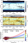 |
Fig. A.1 Statistical analysis of LIR brightness temperature data after removal of thermal tides. Panel (c): Counts of available data. Panel (b): Standard deviation of the tide-removed brightness temperature along the time axis. Panel (c): Zonal brightness temperature anomalies in Fig. 2a (scattered points) as a function of underlying surface elevation. The solid curve in (c) represents a second-order polynomial fit, with shaded areas indicating the root mean squared error. |
Appendix B Background stability field in the Venus PCM
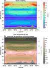 |
Fig. B.1 Temporal and zonal averaged static stability (a) and reciprocal of potential temperature vertical gradient (1/θ̄z, b) in the Venus PCM. Light and dark gray shading indicates, respectively, the maximum and mean surface topography at each latitude. Black contours represent the background zonal wind. |
All Figures
|
Fig. 1 Distribution and smoothing of Akatsuki/LIR data. Panel a : distribution of brightness temperature (gray dots) and derived cloud-tracked winds (cyan dots) as a function of local time and observation date. Black dots indicate the subsolar longitude of each image. The defined Venus date was derived by fitting a sawtooth function to the subsolar longitude. Panels b-d: 1/12 Venus-day means of brightness temperature (b), zonal wind (c), and meridional wind (d). The solid lines represent 5-Venus-day running means applied to each variable. |
| In the text | |
|
Fig. 2 Zonal anomalies of stationary features observed by Akat-suki/LIR. Panels show brightness the temperature (a), zonal wind (b), and meridional wind (c) after a temporal median is applied following thermal tide removal. Color shading indicates zonal anomalies relative to the longitudinal mean at each latitude. Black contours indicate the surface topography at elevations of 1, 3, and 5 km, with major highland regions labeled in panel a. Gray areas indicate regions with insufficient valid data. For the wind (brightness temperature) data, areas left with fewer than 20 (40) valid measurements after the removal of thermal tides are left empty (see Fig. A.1a). |
| In the text | |
|
Fig. 3 Local time dependence of zonal anomalies near Aphrodite Terra (5°S-15°S). Panels show brightness temperatures (a), zonal winds (b), and meridional winds (c) based on observations binned into 2-Venus-hour intervals in defined Venus Universal Time (Venus UT). The resulting fields are projected onto local time-longitude coordinates, and the median value is taken in each bin over the 5°S-15°S latitude band. Color shading indicates deviations from the zonal mean at each local time. |
| In the text | |
|
Fig. 4 Temporal variations of zonal anomalies near Aphrodite Terra (5°S-15°S). A 5-Venus-day Gaussian smoothing is applied along the Venus date axis, followed by thermal tide removal via harmonic fitting at each smoothed field within the 5°S-15°S latitude band. Panel a : brightness temperatures. Panel b : zonal winds. Panel c : meridional winds. Color shading indicates deviations from the zonal mean. The red rectangles indicate the regions where the longitudinal contrasts are reduced over time. Gray areas indicate regions without data. |
| In the text | |
|
Fig. 5 Horizontal structure of stationary waves simulated by the Venus PCM, averaged over 5 Venus days. Panels show air temperatures (a), vertical winds (b), zonal winds (c), and meridional winds (d) at three altitude levels: deep atmosphere (−30 km), lower clouds (~50 km), and cloud top (~70 km). Black contours indicate the underlying surface topography, with elevations corresponding to major highland regions. Undulations on each horizontal slice represent the absolute values of anomalies scaled by two standard deviations (〈X〉′/2σ) to enhance visibility in the 3D perspective. |
| In the text | |
|
Fig. 6 Comparison of horizontal stationary features at the cloud top between the Venus PCM (a, c, and e) and Akatsuki/LIR (b, d, and f), analogous to Figs. 2 and 5 but decomposed using longitudinal filters: low-pass (a and b; wavenumber ≤6), band-pass (c and d; 6 ≤ wavenumber ≤12), and high-pass (e and f; wavenumber ≥12). |
| In the text | |
|
Fig. 7 Vertical structure of stationary waves at latitudes corresponding to Aphrodite Terra (a, c, and e; 10°S) and Ishtar Terra (b, d, and f; 65°N) in the Venus PCM, averaged over 5 Venus days. Panels a and b: zonal anomalies of vertical wind (color shading), overlaid with streamlines of vertical and zonal wind. The vertical wind is normalized at each altitude level for visibility. Panels c and d: scorer parameter. Panels e and f : vertical AM flux associated with stationary waves, calculated as 〈w〉′〈u〉′ cos φ. |
| In the text | |
|
Fig. 8 AM transport (a and b) and adiabatic heating (c and d) associated with stationary waves in the Venus PCM. Panels a and b: EP flux and the vertical flux of AM (arrows; both divided by basic air density), along with the corresponding zonal wind acceleration (color shading). Panels c and d: Adiabatic heating induced by stationary waves and the associated vertical heat flux component. Light and dark gray shading indicates, respectively, the maximum and mean surface topography at each latitude. Black contours represent the background zonal wind (m/s). |
| In the text | |
|
Fig. 9 Local time dependence of zonal anomalies near Aphrodite Terra (5°S-15°S) in the Venus PCM. Panel a : brightness temperature. Panel b: Richardson number and vertical propagation of stationary waves (arrows; −ρ0a〈w〉′〈u〉′ cos φ). Panel c: zonal acceleration induced by stationary waves expressed as |
| In the text | |
|
Fig. A.1 Statistical analysis of LIR brightness temperature data after removal of thermal tides. Panel (c): Counts of available data. Panel (b): Standard deviation of the tide-removed brightness temperature along the time axis. Panel (c): Zonal brightness temperature anomalies in Fig. 2a (scattered points) as a function of underlying surface elevation. The solid curve in (c) represents a second-order polynomial fit, with shaded areas indicating the root mean squared error. |
| In the text | |
|
Fig. B.1 Temporal and zonal averaged static stability (a) and reciprocal of potential temperature vertical gradient (1/θ̄z, b) in the Venus PCM. Light and dark gray shading indicates, respectively, the maximum and mean surface topography at each latitude. Black contours represent the background zonal wind. |
| In the text | |
Current usage metrics show cumulative count of Article Views (full-text article views including HTML views, PDF and ePub downloads, according to the available data) and Abstracts Views on Vision4Press platform.
Data correspond to usage on the plateform after 2015. The current usage metrics is available 48-96 hours after online publication and is updated daily on week days.
Initial download of the metrics may take a while.