| Issue |
A&A
Volume 704, December 2025
|
|
|---|---|---|
| Article Number | L16 | |
| Number of page(s) | 9 | |
| Section | Letters to the Editor | |
| DOI | https://doi.org/10.1051/0004-6361/202557359 | |
| Published online | 12 December 2025 | |
Letter to the Editor
TOI-7510: A solar-analog system of three transiting giant planets near a Laplace resonance chain★
1
Observatoire de Genève, Département d’Astronomie, Université de Genève, Chemin Pegasi 51b, 1290 Versoix, Switzerland
2
Université Côte d’Azur, Laboratoire Lagrange, OCA, CNRS UMR, 7293 Nice, France
3
School of Physics and Astronomy, Monash University, Victoria 3800, Australia
4
Univ. Grenoble Alpes, CNRS, IPAG, F-38000 Grenoble, France
5
Department of Astrophysical Sciences, Princeton University, Princeton, NJ 08544, USA
6
PNRA and IPEV, Concordia Station, Antarctica
7
Instituto Tecnológico de Buenos Aires (ITBA), Iguazú 341, Buenos Aires CABA C1437, Argentina
8
Instituto de Ciencias Físicas (ICIFI; CONICET), ECyT-UNSAM, Buenos Aires, Argentina
9
NASA Ames Research Center, Moffett Field, Mountain View, CA 94035, USA
10
School of Physics & Astronomy, University of Birmingham, Edgbaston, Birmingham B15 2TT, UK
★★ Corresponding author: This email address is being protected from spambots. You need JavaScript enabled to view it.
Received:
22
September
2025
Accepted:
20
November
2025
Abstract
We report the confirmation and initial characterization of a compact and dynamically rich multiple giant planet system orbiting the solar analog TOI-7510. The system was recently identified as a candidate two-planet system in a machine-learning search of the TESS light curves. Using TESS data and photometric follow-up observations with ASTEP, CHEOPS, and EulerCam, we show that one transit was initially misattributed and that the system consists of three transiting giant planets with orbital periods of 11.5, 22.6, and 48.9 days. The planets have radii of 0.65, 0.96, and 0.94 RJ, making them the largest known trio of transiting planets. The system architecture lies near a 4:2:1 mean motion resonant chain, inducing large transit timing variations for all three planets. Photodynamical modeling gives mass estimates of 0.057, 0.41, and 0.60 MJ and favors low eccentricities and mutual inclinations. TOI-7510 is an interesting system for investigating the dynamical interactions and formation histories of compact systems of giant planets.
Key words: stars: individual: TOI-7510 / planetary systems / techniques: photometric / techniques: radial velocities
This study uses CHEOPS data observed as part of the Discretionary Programme (DP) PR450028 (PI Almenara).
© The Authors 2025
 Open Access article, published by EDP Sciences, under the terms of the Creative Commons Attribution License (https://creativecommons.org/licenses/by/4.0), which permits unrestricted use, distribution, and reproduction in any medium, provided the original work is properly cited.
This article is published in open access under the Subscribe to Open model. This email address is being protected from spambots. You need JavaScript enabled to view it. to support open access publication.
1. Introduction
Salinas et al. (2025) recently identified the solar-analog star TOI-7510 (TIC 118798035) as a candidate multiplanet system during a machine learning search of the light curves of the Transiting Exoplanet Survey Satellite (TESS; Ricker et al. 2015). They interpreted the system as containing only two planets. However, the apparent transit-timing variations (TTVs) of the outer planet seemed implausibly large (see Fig. 14 in Salinas et al. 2025). This anomaly drew our attention to the system, so we explored the possibility that one of the observed TESS transits was caused by a third planet.
In this Letter, we confirm three transiting giant planets in the TOI-7510 system with orbital periods of 11.5 days (planet b), 22.6 days (planet c), and 48.9 days (planet d). Their radii are 0.65, 0.96, and 0.94 RJ, respectively, making this system the largest known trio of transiting planets in terms of planetary size. Another notable feature is its compactness. There are only five known systems of three or more giant1 planets that feature period ratios of Pi + 1/Pi ≲ 3, comparable to the outer Solar System: HD 184010 (Teng et al. 2022), HD 34445 (Howard et al. 2010; Vogt et al. 2017), ρ CrB (Noyes et al. 1997; Fulton et al. 2016; Brewer et al. 2023), GJ 876 (Delfosse et al. 1998; Marcy et al. 1998, 2001; Rivera et al. 2010), and now TOI-7510 (see Fig. 1). Because the four other systems are non-transiting, TOI-7510 is the system of choice for studying the processes that shape compact multi-giant systems such as our own. We highlight this system’s orbital architecture, the preliminary constraints we obtained on its planetary masses and eccentricities, and the high potential of the system for further investigation.
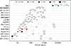 |
Fig. 1. Known systems hosting three or more planets with masses (or minimum masses) between 14 ME and 13 MJ, mass uncertainties below 20%, and orbital period uncertainties below 2%. Open circles indicate planets detected via radial velocity monitoring, while filled circles correspond to transiting planets. The circle sizes are proportional to the logarithm of the planetary mass. Period ratios between adjacent planets are annotated in black or in light gray if Pi + 1/Pi > 3.5. Notably, the inner pair of TOI-7510 has a period ratio of 1.957, similar to the Uranus–Neptune ratio of 1.961. Lower-mass planets in these systems are excluded from the figure. Data were retrieved from the NASA Exoplanet Archive (Akeson et al. 2013). |
2. Observations
TOI-7510 was observed by TESS in four sectors, approximately every two years (see Fig. 2). Due to this sparse temporal coverage, the TESS transits do not uniquely constrain the orbital period of planet d, with its possible values ranging from 38.6 to 733 days. To resolve this ambiguity, we organized a follow-up campaign aimed at capturing two consecutive transits of planet d using the Antarctica Search for Transiting ExoPlanets (ASTEP; Guillot et al. 2015; Mékarnia et al. 2016), the CHaracterising ExOPlanet Satellite (CHEOPS; Benz et al. 2021), and the EulerCam (ECAM; Lendl et al. 2012). We confirmed an orbital period of 48.9 days for planet d. In addition, we acquired 30 radial velocity (RV) measurements with the CORALIE spectrograph (Queloz et al. 2001; Ségransan et al. 2010). Those datasets are described in Appendix A.
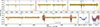 |
Fig. 2. Photodynamical modeling of the transit photometry. The dots, color coded by telescope, represent the noise-model-corrected observations. The black line shows the transit model. Vertical lines mark the midtransit time of planets b (blue), c (orange), and d (green) and are labeled by the number of orbital periods since the first observed transit. |
3. Stellar parameters
To determine the stellar parameters of TOI-7510, we fit its spectral energy distribution (SED; see Appendix B) using stellar atmosphere and evolution models, adopting priors on the distance from the Gaia parallax (Gaia Collaboration 2016, 2023) and on atmospheric parameters from Gaia XP spectra (Andrae et al. 2023a). The derived stellar mass and radius (1.053 ± 0.068 M⊙, 1.030 ± 0.046 R⊙, both within 1 sigma of the Sun) were used as priors in the photodynamical modeling (Sect. 4).
4. Analysis
We jointly fit the observed photometry and RVs using a photodynamical model (Carter et al. 2011) that accounts for the gravitational interactions among the four known bodies in the system (Appendix C). Table D.3 lists the median and the 68% credible interval (CI) of the marginal distribution of the inferred system parameters. Figure 3 presents the posterior TTVs for the three planets, derived from the times of minimum projected separation between the star and planet, and a comparison with the individually determined transit times (Table D.2) computed with juliet (Espinoza et al. 2019; Kreidberg 2015; Speagle 2020), assuming a constant transit duration and the same noise model as in the photodynamical analysis.
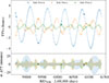 |
Fig. 3. Posterior TTV predictions of planets b (blue band), c (orange band), and d (green band) computed relative to a linear ephemeris (Table D.3). A thousand random draws from the posterior distribution were used to estimate the median TTV values and their uncertainties (68.3% confidence interval). The upper panel shows the posterior TTV values and compares them with the individual transit-time determinations (Table D.2, error bars). In the lower panel, the posterior median transit-timing value was subtracted to emphasize the uncertainty in the distribution and facilitate a clearer comparison with the individually determined transit times. |
5. Results and discussion
Pairs of planets near a mean-motion resonance (MMR) are expected to exhibit TTVs at the superperiod, which for a pair of planets near the k + 1 : k MMR is Psuper = 1/(k/Pin − (k + 1)/Pout). As the 2:1 MMRs is the closest relevant MMR for both pairs of planets, the two expected superperiods are Psuper, bc = 1/(1/Pb − 2/Pc)≈528 days and Psuper, cd = 1/(1/Pc − 2/Pd)≈296 days. Despite the relatively low number of available transits and RV measurements, the large signal to noise ratio of each individual transit observation motivated a photodynamical modeling of the available data (Sect. 4). We note that at this stage, the constraints come mainly from the photometry rather than the RV data due to the limited precision of CORALIE RVs dominated by photon noise for such a star magnitude. As a result, the mass and radius scale of the system is currently set by the stellar mass and radius priors obtained from modeling the star. Figure 3 shows that the periodicities of the TTV model for the inner (b) and outer (d) planets are respectively close to the expected values for Psuper, bc and Psuper, cd, while the TTV model for the middle (c) planet is a sum of contributions at both periods. In addition, a short-term “chopping” effect (Deck et al. 2014) is visible in the TTV model. The observed TTVs are therefore well explained by a three-planet model, supporting our interpretation of the system. Regarding the orbital parameters, the orbital inclinations and longitudes of the ascending node are well constrained and compatible with pairwise mutual inclinations of ≲2°, hinting at a relatively flat system.
Next we consider the constraints on the masses of the planets and their eccentricity vectors (eccentricity and longitude of periastron). The TTV characterization of multi-planetary systems dominated by a signal at the superperiod can be affected by two layers of eccentricity degeneracies: a degeneracy between the mass of the planets and the part of the eccentricities related to the resonant interaction (Boué et al. 2012; Lithwick et al. 2012), and the degeneracy of the non-resonant part of the eccentricities (Leleu et al. 2021). The first degeneracy has been resolved in tens of TTV systems, enabling robust mass measurements (Hadden & Lithwick 2017; Leleu et al. 2023; Almenara et al. 2025), typically by observing the chopping signal, the effect of libration in a resonance (Almenara et al. 2025), or other TTV signals besides the superperiod signals. Resolving the second degeneracy, which also allows for the determination of the full eccentricity vector, is more difficult, and it has only been accomplished for a few systems, notably for planets near 2:1 MMRs with giant planets (Korth et al. 2023, 2024; Borsato et al. 2024). Despite the relatively few observed transits of TOI-7510, the planetary masses appear well constrained, with respective values of 0.057 ± 0.005, 0.41 ± 0.04, and 0.60 ± 0.06 MJ for planets b, c, and d. However, given the relatively low number of data points, the mass determinations are not yet robust, and our fit would, for instance, be largely blind to additional dynamically significant planets in the system. The masses may therefore change once more data are obtained. At this point, the full eccentricity vectors of the planets are not well constrained, although their magnitudes are each below 0.1 in the posterior (see Fig. D.2). Overall, the results of this preliminary study are consistent with general trends in the sub-Neptune population, with planets close to MMRs tending to have lower densities (see Fig. D.1) and smaller mutual inclinations than than those far from resonance (Leleu et al. 2024).
Regarding the system’s architecture, TOI-7510 is the first known system where three transiting giant planets all have radii above 0.65 RJ. In fact, two of the planets are nearly Jupiter-sized. Unlike the more common systems of super-Earths and sub-Neptunes, TOI-7510 hosts higher-mass planets with larger envelope masses, suggesting primordial atmospheres and formation during the disk stage. Figure 1 presents an analogous comparison involving mass rather than radius, as all other known systems of three or more giants are at least partially non-transiting (open circles in the figure). All three planets of TOI-7510 orbit within 0.27 au, well inside Mercury’s orbital distance around the Sun. The three planets must have undergone substantial inward migration since the inner regions of a typical protoplanetary disk would not contain enough mass to form them in situ. The period ratios between the planets largely determine the relevance of their mutual gravitational interactions. Only HD 184010, HD 34445, ρ CrB, GJ 876, and TOI-7510 exhibit compactness comparable to the outer Solar System, with adjacent planets having period ratios ≲3. Thus, constraining the current orbital architecture of these systems can lead to better understanding of the physical processes that shaped them in the past, for example, whether the architectures are consistent with formation and migration in the proto-planetary disk and indeed whether they have signatures of post-disk gravitational instabilities (e.g., Izidoro et al. 2017; Li et al. 2025).
Moreover, the period ratios 1.96 and 2.17 for the inner and outer pairs are worth commenting on in this preliminary investigation, especially from the point of view of the formation of a three-planet system composed of a Neptune interior to two gas giants. Studies of planet-disk interactions distinguish between Type I and Type II migration for low- and high-mass planets, respectively, with the latter involving disk clearing in the vicinity of the planet, which in turn results in migration timescales that are considerably longer than for Type I. One can therefore conceive of a situation where planet b arrives at the disk edge ahead of the two giants, and in the meantime, the two giants experience resonant repulsion via mutual density wave emission as they migrate inward (Podlewska-Gaca et al. 2012; Baruteau & Papaloizou 2013; Cui et al. 2021). Since resonance capture normally occurs at period ratios larger than exact commensurability and systems that are not captured move on to the next strong resonance, a period ratio slightly less than commensurability for the inner pair suggests some interesting planet-disk dynamics not readily described by simple migration models.
With three transiting giant planets near a 4:2:1 Laplace resonance chain with peak-to-peak TTV amplitudes of 1 to 7 hours at the superperiod signal and a typical timing precision of 1 to 3 minutes, TOI-7510 is an excellent candidate for in-depth TTV characterization of its planetary masses and orbital parameters, including the full eccentricity vectors. This should be enabled by the additional TESS observations scheduled for April 21 to June 13, 2026 (sectors 103 and 104), as well as by the future ground- and space-based photometric follow-up. The star is bright enough (G = 11.8 mag) for high-precision RV monitoring on an 8 m class telescope, which will help determine precise absolute masses and radii without needing to rely on stellar evolutionary models (Agol et al. 2005; Almenara et al. 2015).
The planets exhibit low bulk densities and moderate stellar insolation, with equilibrium temperatures between 540 and 880 K. Their co-evolution allows for a refined study of their bulk composition (Havel et al. 2011), while their moderate equilibrium temperatures imply that inflation from Ohmic dissipation should be limited (Thorngren et al. 2016). With its extremely low density, planet b is particularly intriguing, and it is another example of a so-called super-puff planet (Masuda 2014), probably with a small core and a highly extended H/He envelope. Owing to its low density and moderately high equilibrium temperature, planet b has a transmission spectroscopy metric (Kempton et al. 2018) of 155 ± 17, above the suggested threshold for atmospheric follow-up. The characterization of the atmospheres of planets in this intriguing near-resonant system should shed light on planetary formation in general.
Data availability
Samples from the posterior, transit times forecast, and datasets are available at https://zenodo.org/records/17662413.
Here, we define a giant as a planet ≥ 14 M⊕ in order to exclude most of the sub-Neptune population.
BJDTDB times for the target observations were computed following https://github.com/havijw/tess-time-correction.
We adopted a solar-scaled composition, assuming [α/Fe] = 0.0 dex.
Acknowledgments
This paper uses data obtained with the ASTEP telescope, at Concordia Station in Antarctica. ASTEP benefited from the support of the French and Italian polar agencies IPEV and PNRA in the framework of the Concordia station program, from OCA, INSU, Idex UCAJEDI (ANR- 15-IDEX-01) and ESA through the Science Faculty of the European Space Research and Technology Centre (ESTEC). The Birmingham contribution to ASTEP is supported by the European Union’s Horizon 2020 research and innovation programme (grant’s agreement n° 803193/BEBOP), and from the Science and Technology Facilities Council (STFC; grant n° ST/S00193X/1, and ST/W002582/1). This paper includes data collected by the TESS mission. Funding for the TESS mission is provided by the NASA’s Science Mission Directorate. Resources supporting this work were provided by the NASA High-End Computing (HEC) Program through the NASA Advanced Supercomputing (NAS) Division at Ames Research Center for the production of the SPOC data products. This paper includes data collected by the TESS mission that are publicly available from the Mikulski Archive for Space Telescopes (MAST). CHEOPS is an ESA mission in partnership with Switzerland with important contributions to the payload and the ground segment from Austria, Belgium, France, Germany, Hungary, Italy, Portugal, Spain, Sweden, and the United Kingdom. The CHEOPS Consortium would like to gratefully acknowledge the support received by all the agencies, offices, universities, and industries involved. Their flexibility and willingness to explore new approaches were essential to the success of this mission. CHEOPS data analysed in this article will be made available in the CHEOPS mission archive (https://cheops.unige.ch/archive_browser/). This work is based on observations collected with the CORALIE echelle spectrograph and EulerCam mounted on the 1.2 m Swiss Euler telescope at La Silla Observatory, Chile. This work has made use of data from the European Space Agency (ESA) mission Gaia (https://www.cosmos.esa.int/gaia), processed by the Gaia Data Processing and Analysis Consortium (DPAC, https://www.cosmos.esa.int/web/gaia/dpac/consortium). Funding for the DPAC has been provided by national institutions, in particular the institutions participating in the Gaia Multilateral Agreement. Simulations in this paper made use of the REBOUND code which can be downloaded freely at http://github.com/hannorein/rebound. These simulations have been run on the Bonsai cluster kindly provided by the Observatoire de Genève. A.L., J.K, and J.M.A. acknowledges support of the Swiss National Science Foundation under grant number TMSGI2_211697. M.L. acknowledges support of the Swiss National Science Foundation under grant number PCEFP2_194576. This work has been carried out within the framework of the NCCR PlanetS supported by the Swiss National Science Foundation under grant 51NF40_205606.
References
- Agol, E., Steffen, J., Sari, R., & Clarkson, W. 2005, MNRAS, 359, 567 [Google Scholar]
- Akeson, R. L., Chen, X., Ciardi, D., et al. 2013, PASP, 125, 989 [Google Scholar]
- Allard, F., Homeier, D., & Freytag, B. 2012, Philos. Trans. Royal Soc. London Ser. A, 370, 2765 [Google Scholar]
- Almenara, J. M., Díaz, R. F., Mardling, R., et al. 2015, MNRAS, 453, 2644 [Google Scholar]
- Almenara, J. M., Mardling, R., Leleu, A., et al. 2025, A&A, 703, A167 [NASA ADS] [CrossRef] [EDP Sciences] [Google Scholar]
- Andrae, R., Fouesneau, M., Sordo, R., et al. 2023a, A&A, 674, A27 [CrossRef] [EDP Sciences] [Google Scholar]
- Andrae, R., Rix, H.-W., & Chandra, V. 2023b, ApJS, 267, 8 [NASA ADS] [CrossRef] [Google Scholar]
- Astropy Collaboration (Price-Whelan, A. M., et al.) 2022, ApJ, 935, 167 [NASA ADS] [CrossRef] [Google Scholar]
- Baranne, A., Queloz, D., Mayor, M., et al. 1996, A&AS, 119, 373 [NASA ADS] [CrossRef] [EDP Sciences] [Google Scholar]
- Baruteau, C., & Papaloizou, J. C. B. 2013, ApJ, 778, 7 [NASA ADS] [CrossRef] [Google Scholar]
- Benz, W., Broeg, C., Fortier, A., et al. 2021, Exp. Astron., 51, 109 [Google Scholar]
- Borsato, L., Degen, D., Leleu, A., et al. 2024, A&A, 689, A52 [NASA ADS] [CrossRef] [EDP Sciences] [Google Scholar]
- Boué, G., Oshagh, M., Montalto, M., & Santos, N. C. 2012, MNRAS, 422, L57 [NASA ADS] [Google Scholar]
- Bradley, L. 2023, https://doi.org/10.5281/zenodo.7946442 [Google Scholar]
- Brandeker, A., Patel, J. A., & Morris, B. M. 2024, Astrophysics Source Code Library [record ascl:2404.002] [Google Scholar]
- Brasseur, C. E., Phillip, C., Fleming, S. W., Mullally, S. E., & White, R. L. 2019, Astrophysics Source Code Library [record ascl:1905.007] [Google Scholar]
- Brewer, J. M., Zhao, L. L., Fischer, D. A., et al. 2023, AJ, 166, 46 [Google Scholar]
- Broeg, C., Fernández, M., & Neuhäuser, R. 2005, Astron. Nachr., 326, 134 [NASA ADS] [CrossRef] [Google Scholar]
- Caldwell, D. A., Tenenbaum, P., Twicken, J. D., et al. 2020, Res. Notes Am. Astron. Soc., 4, 201 [Google Scholar]
- Carter, J. A., Fabrycky, D. C., Ragozzine, D., et al. 2011, Science, 331, 562 [NASA ADS] [CrossRef] [Google Scholar]
- Chen, Y., Girardi, L., Bressan, A., et al. 2014, MNRAS, 444, 2525 [Google Scholar]
- Cui, Z., Papaloizou, J. C. B., & Szuszkiewicz, E. 2021, ApJ, 921, 142 [Google Scholar]
- Cutri, R. M., Skrutskie, M. F., van Dyk, S., et al. 2003, VizieR Online Data Catalog: II/246 [Google Scholar]
- Cutri, R. M., Wright, E. L., Conrow, T., et al. 2021, VizieR On-line Data Catalog: II/328 [Google Scholar]
- Deck, K. M., Agol, E., Holman, M. J., & Nesvorný, D. 2014, ApJ, 787, 132 [CrossRef] [Google Scholar]
- Delfosse, X., Forveille, T., Mayor, M., et al. 1998, A&A, 338, L67 [Google Scholar]
- Díaz, R. F., Almenara, J. M., Santerne, A., et al. 2014, MNRAS, 441, 983 [Google Scholar]
- Dotter, A., Chaboyer, B., Jevremović, D., et al. 2008, ApJS, 178, 89 [Google Scholar]
- Espinoza, N., Kossakowski, D., & Brahm, R. 2019, MNRAS, 490, 2262 [Google Scholar]
- Fausnaugh, M. M., Burke, C. J., Ricker, G. R., & Vanderspek, R. 2020, Res. Notes Am. Astron. Soc., 4, 251 [Google Scholar]
- Foreman-Mackey, D., Hogg, D. W., Lang, D., & Goodman, J. 2013, PASP, 125, 306 [Google Scholar]
- Foreman-Mackey, D., Agol, E., Ambikasaran, S., & Angus, R. 2017, AJ, 154, 220 [Google Scholar]
- Fulton, B. J., Howard, A. W., Weiss, L. M., et al. 2016, ApJ, 830, 46 [NASA ADS] [Google Scholar]
- Gaia Collaboration (Prusti, T., et al.) 2016, A&A, 595, A1 [NASA ADS] [CrossRef] [EDP Sciences] [Google Scholar]
- Gaia Collaboration (Vallenari, A., et al.) 2023, A&A, 674, A1 [NASA ADS] [CrossRef] [EDP Sciences] [Google Scholar]
- Garcia, L. J., Timmermans, M., Pozuelos, F. J., et al. 2022, MNRAS, 509, 4817 [Google Scholar]
- Goodman, J., & Weare, J. 2010, Commun. Appl. math. Computat. Sci., 5, 65 [Google Scholar]
- Gregory, P. C. 2005, ApJ, 631, 1198 [NASA ADS] [CrossRef] [Google Scholar]
- Guillot, T., Abe, L., Agabi, A., et al. 2015, Astron. Nachr., 336, 638 [NASA ADS] [CrossRef] [Google Scholar]
- Hadden, S., & Lithwick, Y. 2017, AJ, 154, 5 [Google Scholar]
- Havel, M., Guillot, T., Valencia, D., & Crida, A. 2011, A&A, 531, A3 [Google Scholar]
- Høg, E., Fabricius, C., Makarov, V. V., et al. 2000, A&A, 355, L27 [Google Scholar]
- Howard, A. W., Johnson, J. A., Marcy, G. W., et al. 2010, ApJ, 721, 1467 [Google Scholar]
- Hoyer, S., Guterman, P., Demangeon, O., et al. 2020, A&A, 635, A24 [NASA ADS] [CrossRef] [EDP Sciences] [Google Scholar]
- Irwin, J. B. 1952, ApJ, 116, 211 [Google Scholar]
- Izidoro, A., Ogihara, M., Raymond, S. N., et al. 2017, MNRAS, 470, 1750 [Google Scholar]
- Jenkins, J. M., Twicken, J. D., McCauliff, S., et al. 2016, SPIE Conf. Ser., 9913, 99133E [Google Scholar]
- Kempton, E. M. R., Bean, J. L., Louie, D. R., et al. 2018, PASP, 130, 114401 [Google Scholar]
- Kipping, D. M. 2010, MNRAS, 408, 1758 [Google Scholar]
- Korth, J., Gandolfi, D., Šubjak, J., et al. 2023, A&A, 675, A115 [NASA ADS] [CrossRef] [EDP Sciences] [Google Scholar]
- Korth, J., Chaturvedi, P., Parviainen, H., et al. 2024, ApJ, 971, L28 [NASA ADS] [CrossRef] [Google Scholar]
- Kreidberg, L. 2015, PASP, 127, 1161 [Google Scholar]
- Leleu, A., Chatel, G., Udry, S., et al. 2021, A&A, 655, A66 [CrossRef] [Google Scholar]
- Leleu, A., Delisle, J. B., Udry, S., et al. 2023, A&A, 669, A117 [NASA ADS] [CrossRef] [EDP Sciences] [Google Scholar]
- Leleu, A., Delisle, J.-B., Burn, R., et al. 2024, A&A, 687, L1 [NASA ADS] [CrossRef] [EDP Sciences] [Google Scholar]
- Lendl, M. 2014, Ph.D Thesis, University of Geneva, Switzerland [Google Scholar]
- Lendl, M., Anderson, D. R., Collier-Cameron, A., et al. 2012, A&A, 544, A72 [NASA ADS] [CrossRef] [EDP Sciences] [Google Scholar]
- Li, R., Chiang, E., Choksi, N., & Dai, F. 2025, AJ, 169, 323 [Google Scholar]
- Lightkurve Collaboration (Cardoso, J. V. d. M., et al.) 2018, Astrophysics Source Code Library [record ascl:1812.013] [Google Scholar]
- Lindegren, L., Klioner, S. A., Hernández, J., et al. 2021, A&A, 649, A2 [EDP Sciences] [Google Scholar]
- Lithwick, Y., Xie, J., & Wu, Y. 2012, ApJ, 761, 122 [Google Scholar]
- Marcy, G. W., Butler, R. P., Vogt, S. S., Fischer, D., & Lissauer, J. J. 1998, ApJ, 505, L147 [Google Scholar]
- Marcy, G. W., Butler, R. P., Fischer, D., et al. 2001, ApJ, 556, 296 [Google Scholar]
- Masuda, K. 2014, ApJ, 783, 53 [Google Scholar]
- Mékarnia, D., Guillot, T., Rivet, J. P., et al. 2016, MNRAS, 463, 45 [Google Scholar]
- Mowlavi, N., Holl, B., Lecoeur-Taïbi, I., et al. 2023, A&A, 674, A16 [NASA ADS] [CrossRef] [EDP Sciences] [Google Scholar]
- Noyes, R. W., Jha, S., Korzennik, S. G., et al. 1997, ApJ, 483, L111 [NASA ADS] [CrossRef] [Google Scholar]
- Parc, L., Bouchy, F., Venturini, J., Dorn, C., & Helled, R. 2024, A&A, 688, A59 [NASA ADS] [CrossRef] [EDP Sciences] [Google Scholar]
- Pecaut, M. J., & Mamajek, E. E. 2013, ApJS, 208, 9 [Google Scholar]
- Pepe, F., Mayor, M., Galland, F., et al. 2002, A&A, 388, 632 [NASA ADS] [CrossRef] [EDP Sciences] [Google Scholar]
- Podlewska-Gaca, E., Papaloizou, J. C. B., & Szuszkiewicz, E. 2012, MNRAS, 421, 1736 [Google Scholar]
- Queloz, D., Mayor, M., Udry, S., et al. 2001, The Messenger, 105, 1 [NASA ADS] [Google Scholar]
- Rein, H., & Liu, S. F. 2012, A&A, 537, A128 [NASA ADS] [CrossRef] [EDP Sciences] [Google Scholar]
- Rein, H., & Tamayo, D. 2015, MNRAS, 452, 376 [Google Scholar]
- Ricker, G. R., Winn, J. N., Vanderspek, R., et al. 2015, J. Astron. Telescopes Instrum. Syst., 1, 014003 [Google Scholar]
- Riello, M., De Angeli, F., Evans, D. W., et al. 2021, A&A, 649, A3 [NASA ADS] [CrossRef] [EDP Sciences] [Google Scholar]
- Rivera, E. J., Laughlin, G., Butler, R. P., et al. 2010, ApJ, 719, 890 [Google Scholar]
- Salinas, H., Brahm, R., Olmschenk, G., et al. 2025, MNRAS, 538, 2031 [Google Scholar]
- Schmider, F.-X., Abe, L., Agabi, A., et al. 2022, SPIE Conf. Ser., 12182, 121822O [NASA ADS] [Google Scholar]
- Ségransan, D., Udry, S., Mayor, M., et al. 2010, A&A, 511, A45 [NASA ADS] [CrossRef] [EDP Sciences] [Google Scholar]
- Skrutskie, M. F., Cutri, R. M., Stiening, R., et al. 2006, AJ, 131, 1163 [NASA ADS] [CrossRef] [Google Scholar]
- Smith, J. C., Stumpe, M. C., Van Cleve, J. E., et al. 2012, PASP, 124, 1000 [Google Scholar]
- Speagle, J. S. 2020, MNRAS, 493, 3132 [Google Scholar]
- Stassun, K. G., Oelkers, R. J., Paegert, M., et al. 2019, AJ, 158, 138 [Google Scholar]
- Stumpe, M. C., Smith, J. C., Van Cleve, J. E., et al. 2012, PASP, 124, 985 [Google Scholar]
- Stumpe, M. C., Smith, J. C., Catanzarite, J. H., et al. 2014, PASP, 126, 100 [Google Scholar]
- Tayar, J., Claytor, Z. R., Huber, D., & van Saders, J. 2022, ApJ, 927, 31 [NASA ADS] [CrossRef] [Google Scholar]
- Teng, H.-Y., Sato, B., Takarada, T., et al. 2022, PASJ, 74, 1309 [Google Scholar]
- Thorngren, D. P., Fortney, J. J., Murray-Clay, R. A., & Lopez, E. D. 2016, ApJ, 831, 64 [NASA ADS] [CrossRef] [Google Scholar]
- Twicken, J. D., Catanzarite, J. H., Clarke, B. D., et al. 2018, PASP, 130, 064502 [Google Scholar]
- Vogt, S. S., Butler, R. P., Burt, J., et al. 2017, AJ, 154, 181 [NASA ADS] [CrossRef] [Google Scholar]
- Wright, E. L., Eisenhardt, P. R. M., Mainzer, A. K., et al. 2010, AJ, 140, 1868 [Google Scholar]
- Zechmeister, M., & Kürster, M. 2009, A&A, 496, 577 [CrossRef] [EDP Sciences] [Google Scholar]
Appendix A: Datasets
A.1. TESS
TESS (Ricker et al. 2015) observed TOI-7510 in full-frame images (FFIs) during Sectors 13, 39, 66, and 93, with cadences of 1800, 600, 200 and 200 seconds, respectively. For Sectors 13 and 39, we used the presearch data-conditioning simple aperture photometry (PDCSAP; Smith et al. 2012, Stumpe et al. 2012, 2014) light curves of TOI-7510, produced by the TESS Science Processing Operations Center (SPOC; Jenkins et al. 2016; Caldwell et al. 2020). For sectors 66 and 93, we produced light curves using TESSCut (Brasseur et al. 2019) from FFIs calibrated by SPOC, and performed photometry with the Lightkurve package (Lightkurve Collaboration 2018)2. Prior to the availability of SPOC-calibrated FFIs for Sector 93, we also made use of the TESS Image CAlibrator Full Frame Images (TICA; Fausnaugh et al. 2020). The SPOC detected the transit signature of planet c at an orbital period of 22.572 days in a search of Sector 39, and second candidate transit signal at 4.666 days consisting of one transit of planet b with the single transit of planet d. Planet c’s signature passed all the data validation diagnostic tests (Twicken et al. 2018), while the diagnostic tests for the planet b/d transits were compromised by the erroneous orbital period. TESS photometry is contaminated by the nearby eclipsing binary Gaia DR3 6652375098458686720, which has a period of 1.36 days (Mowlavi et al. 2023).
A.2. ASTEP
ASTEP is a 0.4 m telescope equipped with a Wynne Newtonian coma corrector, located at Dome C on the east Antarctic plateau (Guillot et al. 2015; Mékarnia et al. 2016). The focal box hosts two high-sensitivity cameras at red and blue wavelengths (Schmider et al. 2022). ASTEP observations of TOI-7510 were scheduled on June 16 and 17, 2025, continuously, to attempt to detect planet d whose period, between 38.6 and 733 days, was very uncertain at this point. TESS was observing the target during this period, but a programmed 5-hour data downlink meant the possibility of missing the transit. The transit of planet d on 2025-06-17 was observed simultaneously and with consistent depths, with ASTEP in band B and band R and TESS. This helped refine the set of 19 possible aliases for the next transit of planet d. Four of these aliases (#19, 18, 17, and 16) were observed by ASTEP on July 25, 28, and 30, 2025, and August 1, 2025, and ruled out. On August 5, 2025, because of the shorter night, ASTEP could only observe after the predicted egress of alias #15, whose transit was detected by CHEOPS and EulerCam (see below). In addition, ASTEP observed achromatic transits of planet c on June 26 and September 2, 2025.
A.3. CHEOPS
CHEOPS (Benz et al. 2021) observed a partial transit of planet d on August 4, 2025 (Table A.1). The raw data was automatically processed by the CHEOPS data reduction pipeline (DRP; version 15.1.1; Hoyer et al. 2020). We performed point-spread function photometry with the PIPE package3 (Brandeker et al. 2024).
CHEOPS observations.
A.4. EulerCam
We observed a transit of planet d, simultaneously with CHEOPS, on August 4, 2025, using EulerCam (ECAM; Lendl et al. 2012) on the Swiss 1.2 m Euler telescope at La Silla Observatory. The night was cloudy, and the egress occurred at high airmass. Observations were conducted with the r’-Gunn filter, using exposure times ranging from 30 to 90 seconds. The image reduction was carried out following Lendl et al. (2012) and Lendl (2014). Aperture photometry was performed using prose (Garcia et al. 2022), which relies on astropy (Astropy Collaboration 2022) and photutils (Bradley 2023). The optimal differential photometry followed Broeg et al. (2005).
A.5. CORALIE
TOI-7510 was observed with the CORALIE spectrograph (Queloz et al. 2001; Ségransan et al. 2010) on the Swiss 1.2 m Euler telescope at La Silla Observatory, Chile, between 2025 June 5 and September 14. CORALIE is a fiber-fed echelle spectrograph with a 2″ science fiber, and a secondary fiber with a Fabry–Perot for simultaneous drift measurement. It has a spectral resolution of R∼60,000. In total, 30 spectra were obtained with a median exposure duration of 45 minutes and a median signal to noise ratio at 550 nm of 11. RVs are extracted using the standard CORALIE DRS-3.8 by cross-correlating the spectra with a binary G2V mask (Baranne et al. 1996; Pepe et al. 2002). The resulting RVs, with a median error of 33 m s−1, are shown in Fig. C.3 and listed in Table A.2. The BIS, FWHM, and other line-profile diagnostics were also computed, as was the Hα index for each spectrum to check for possible variation in stellar activity. The observation on June 11, 2025, was excluded from the analysis because the spectrum was contaminated by the full Moon located 35° from the target.
CORALIE RV measurements.
Appendix B: SED
The SED was constructed using photometric data from Gaia Data Release 3 (DR3; Riello et al. 2021), the 2-Micron All-Sky Survey (2MASS; Skrutskie et al. 2006; Cutri et al. 2003), and the Wide-field Infrared Survey Explorer (WISE; Wright et al. 2010; Cutri et al. 2021). The corresponding measurements are listed in Table D.1. We adopted the PHOENIX/BT-Settl atmosphere model (Allard et al. 2012), along with two sets of stellar evolution models: Dartmouth (Dotter et al. 2008) and PARSEC (Chen et al. 2014). The SED fitting followed the procedure described by Díaz et al. (2014), using informative priors for the effective temperature, surface gravity, and metallicity,4 from (Andrae et al. 2023b). The distance prior was based on the Gaia zeropoint-corrected parallax (Lindegren et al. 2021). Uniform priors were adopted for the remaining parameters. We included a jitter term (Gregory 2005) for each photometric band set (Gaia, 2MASS, and WISE). The posterior median values for the stellar radius are identical for both stellar evolution models, while the stellar mass differs by 0.007 M⊙. We merged the results from the two models assuming equal probability for each. The priors and posteriors for all parameters are listed in Table B.1, and the maximum a posteriori (MAP) stellar atmosphere model is shown in Fig. B.1. Following Tayar et al. (2022), we added a systematic uncertainty floor of 4.2% for the radius and 5% for the mass, combined in quadrature with the statistical uncertainties (Table D.1).
Modeling of the SED.
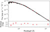 |
Fig. B.1. Spectral energy distribution of TOI-7510. The solid line shows the MAP PHOENIX/BT-Settl interpolated synthetic spectrum, red circles are the absolute photometric observations, and gray open circles are the result of integrating the synthetic spectrum in the observed bandpasses. The lower panel shows the residuals of the MAP model, with the jitter added quadratically to the data error bars. |
Appendix C: Photodynamical modeling
The positions and velocities of the four bodies assumed in the system were computed as a function of time using the n-body code REBOUND (Rein & Liu 2012) employing the WHFast integrator (Rein & Tamayo 2015) with a time step of 0.02 days. The sky-projected positions were used to generate the light curve with batman (Kreidberg 2015), incorporating the light-time effect (Irwin 1952). Oversampling was applied to the TESS data to account for the integration-induced distortion described by Kipping (2010). The line-of-sight velocity of the star, derived from the n-body integration, was used to model the RV measurements. The model was parameterized using the stellar mass and radius, limb-darkening coefficients, planet-to-star mass and radius ratios, and Jacobi orbital elements (Table D.3) at the reference epoch (tref). Due to the symmetry of the problem, we fixed the longitude of the ascending node of planet c at tref to 180°, and constrained the inclination of planet d to be less than 90°. We modeled the error terms of the transit light curves using Gaussian process regression, adopting the approximate Matern kernel implemented in celerite (Foreman-Mackey et al. 2017). We used different kernel hyperparameters for each photometry dataset, corresponding to the individual panels in Fig. C.1. For the CHEOPS observation, we included a linear model with a log-background term and a sine-of-roll-angle component. For
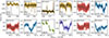 |
Fig. C.1. Photodynamical modeling of the transit photometry. Each dataset is shown in a different panel, labeled with the midtransit date (or the start date of the observation for TESS) and the telescope (or instrument). The error bars, in different colors for each telescope (same color code as in Fig. 2), represent the observations. The black line is the MAP model that combines both transits and noise, while the gray line shows the pure transit model. |
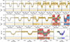 |
Fig. C.2. Noise-model-corrected transits of planets b (first row), c (second row), and d (third row), shown as dots with the same color code as in Fig. 2. The MAP model (black line) and the continuous oversampled MAP model (gray line) from the photodynamical modeling are also shown. Each panel is centered at the linear ephemeris (indicated by the vertical gray lines). Each panel is labeled with the telescopes that observed and the epoch number. The residuals after subtracting the MAP model are shown in the lower part of each panel. |
the ECAM transit, we added linear models in the point spread function centroid shifts and the full width at half maximum. The model for the RV has two additional parameters: the systemic velocity and a jitter term. In total, the model comprises 66 free parameters. We adopted normal priors for the stellar mass and radius from Sect. 3, and uninformative priors for the remaining parameters. The joint posterior distribution was sampled using the emcee algorithm (Goodman & Weare 2010); emcee, with a Gaussian likelihood function and using 660 walkers.
The MAP model for the transit photometry and RV data is plotted in Figs. C.1, and C.3, respectively. Noise-model-corrected datasets and transits for each planet are shown in Figs. 2 and C.2, respectively.
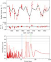 |
Fig. C.3. Top panel: CORALIE RVs of TOI-7510 (red error bars) together with the median RV model (black line) and the 68.3% confidence interval (gray region), both estimated from a thousand random draws from the posterior distribution. Residuals from the median model are shown. Bottom panel: Periodogram of the CORALIE RVs. The red line represents the Generalised Lomb–Scargle periodogram (Zechmeister & Kürster 2009). The gray horizontal lines represent 10, 1, and 0.1% false-alarm levels, from bottom to top. The vertical blue, orange, and green lines respectively mark the period of the transiting planets b, c, and d. |
Appendix D: Additional figures and tables
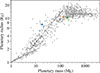 |
Fig. D.1. Mass–radius diagram of known exoplanets. Gray dots are transiting planets listed in the NASA Exoplanet Archive with planetary radius and mass uncertainties below 20%. The dashed black lines are the mass–radius relations from Parc et al. (2024). The Solar System’s giant planets are indicated by their initials (J, S, U, N). |
Astrometry, photometry, and stellar parameters for TOI-7510.
Transit times of the observations.
Inferred system parameters.
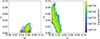 |
Fig. D.2. Pairwise joint posterior distributions of the eccentricities for planets b, c, and d. The dots represent the posterior samples at tref, with the color scale showing their log-posterior value. The evolution during the observations for a thousand random draws from the posterior distribution is shown in light gray (red for the MAP model). |
All Tables
All Figures
|
Fig. 1. Known systems hosting three or more planets with masses (or minimum masses) between 14 ME and 13 MJ, mass uncertainties below 20%, and orbital period uncertainties below 2%. Open circles indicate planets detected via radial velocity monitoring, while filled circles correspond to transiting planets. The circle sizes are proportional to the logarithm of the planetary mass. Period ratios between adjacent planets are annotated in black or in light gray if Pi + 1/Pi > 3.5. Notably, the inner pair of TOI-7510 has a period ratio of 1.957, similar to the Uranus–Neptune ratio of 1.961. Lower-mass planets in these systems are excluded from the figure. Data were retrieved from the NASA Exoplanet Archive (Akeson et al. 2013). |
| In the text | |
|
Fig. 2. Photodynamical modeling of the transit photometry. The dots, color coded by telescope, represent the noise-model-corrected observations. The black line shows the transit model. Vertical lines mark the midtransit time of planets b (blue), c (orange), and d (green) and are labeled by the number of orbital periods since the first observed transit. |
| In the text | |
|
Fig. 3. Posterior TTV predictions of planets b (blue band), c (orange band), and d (green band) computed relative to a linear ephemeris (Table D.3). A thousand random draws from the posterior distribution were used to estimate the median TTV values and their uncertainties (68.3% confidence interval). The upper panel shows the posterior TTV values and compares them with the individual transit-time determinations (Table D.2, error bars). In the lower panel, the posterior median transit-timing value was subtracted to emphasize the uncertainty in the distribution and facilitate a clearer comparison with the individually determined transit times. |
| In the text | |
|
Fig. B.1. Spectral energy distribution of TOI-7510. The solid line shows the MAP PHOENIX/BT-Settl interpolated synthetic spectrum, red circles are the absolute photometric observations, and gray open circles are the result of integrating the synthetic spectrum in the observed bandpasses. The lower panel shows the residuals of the MAP model, with the jitter added quadratically to the data error bars. |
| In the text | |
|
Fig. C.1. Photodynamical modeling of the transit photometry. Each dataset is shown in a different panel, labeled with the midtransit date (or the start date of the observation for TESS) and the telescope (or instrument). The error bars, in different colors for each telescope (same color code as in Fig. 2), represent the observations. The black line is the MAP model that combines both transits and noise, while the gray line shows the pure transit model. |
| In the text | |
|
Fig. C.2. Noise-model-corrected transits of planets b (first row), c (second row), and d (third row), shown as dots with the same color code as in Fig. 2. The MAP model (black line) and the continuous oversampled MAP model (gray line) from the photodynamical modeling are also shown. Each panel is centered at the linear ephemeris (indicated by the vertical gray lines). Each panel is labeled with the telescopes that observed and the epoch number. The residuals after subtracting the MAP model are shown in the lower part of each panel. |
| In the text | |
|
Fig. C.3. Top panel: CORALIE RVs of TOI-7510 (red error bars) together with the median RV model (black line) and the 68.3% confidence interval (gray region), both estimated from a thousand random draws from the posterior distribution. Residuals from the median model are shown. Bottom panel: Periodogram of the CORALIE RVs. The red line represents the Generalised Lomb–Scargle periodogram (Zechmeister & Kürster 2009). The gray horizontal lines represent 10, 1, and 0.1% false-alarm levels, from bottom to top. The vertical blue, orange, and green lines respectively mark the period of the transiting planets b, c, and d. |
| In the text | |
|
Fig. D.1. Mass–radius diagram of known exoplanets. Gray dots are transiting planets listed in the NASA Exoplanet Archive with planetary radius and mass uncertainties below 20%. The dashed black lines are the mass–radius relations from Parc et al. (2024). The Solar System’s giant planets are indicated by their initials (J, S, U, N). |
| In the text | |
|
Fig. D.2. Pairwise joint posterior distributions of the eccentricities for planets b, c, and d. The dots represent the posterior samples at tref, with the color scale showing their log-posterior value. The evolution during the observations for a thousand random draws from the posterior distribution is shown in light gray (red for the MAP model). |
| In the text | |
Current usage metrics show cumulative count of Article Views (full-text article views including HTML views, PDF and ePub downloads, according to the available data) and Abstracts Views on Vision4Press platform.
Data correspond to usage on the plateform after 2015. The current usage metrics is available 48-96 hours after online publication and is updated daily on week days.
Initial download of the metrics may take a while.