| Issue |
A&A
Volume 705, January 2026
|
|
|---|---|---|
| Article Number | A78 | |
| Number of page(s) | 17 | |
| Section | Catalogs and data | |
| DOI | https://doi.org/10.1051/0004-6361/202554997 | |
| Published online | 06 January 2026 | |
Dwarf galaxies within the Kilo Degree Survey
1
Space physics and Astronomy Research Unit, University of Oulu,
Pentti Kaiteran katu 1,
90014
Oulu,
Finland
2
Institute of Astronomy,
Madingley Rd,
Cambridge
CB3 0HA,
UK
3
Visiting Fellow, Clare Hall, University of Cambridge,
Cambridge,
UK
4
Institute of Physics, Laboratory of Astrophysics, Ecole Polytechnique Fédérale de Lausanne (EPFL),
1290 Sauverny,
Switzerland
★ Corresponding author: This email address is being protected from spambots. You need JavaScript enabled to view it.
Received:
2
April
2025
Accepted:
5
November
2025
Abstract
Context. Constraining the properties, spatial distribution, and luminosity function of dwarf galaxies in different galactic environments is crucial for understanding the dwarf galaxy formation and evolution. Large surveys such as the Kilo Degree Survey (KiDS) provide useful publicly available datasets that can be used to identify dwarf galaxy candidates in a range of galactic neighborhoods. The resulting catalogs are useful for constraining the abundance of dwarfs in different environments and also provide useful galaxy samples for future follow-up studies. Ultimately this analysis of low-mass galaxies also provides constraints on our cosmological galaxy formation models.
Aims. We generated a dwarf galaxy candidate catalog based on the KiDS images. KiDS data covers a 1004 deg2 area in u′, g′, r′, and i′ filters that is centered on two horizontal stripes at the equator and in the southern hemisphere. In our catalog we provide the locations, photometric properties, and visual classifications of dwarf galaxy candidates within 60 Mpc in all different environments covered by the KiDS. We also use the catalog to analyze the dwarf galaxy numbers and distributions in groups as a function of groups’ virial mass.
Methods. We used Max-Tree Objects (MTO) to identify sources from the KiDS data. We then selected objects based on their detection sizes and surface brightness. We used automated photometric pipeline to run GALFIT on the images in order to measure the structure, brightness, and color of the objects. We then used size, surface brightness, and color cuts to exclude the likely background galaxies and classify the likelihoods of the remaining objects being dwarf galaxies based on their visual appearance. We also probed the completeness limits and detection biases of our detection procedure, by embedding simulated galaxies into the KiDS images.
Results. Our catalog contains galaxies that have Re larger than 3 arcsec and reaches the 50% completeness limit at the r′-band mean effective surface brightness of 26 mag arcsec−2. Near the completeness limit there is a slight selection bias toward detecting more round and centrally peaked objects more effectively than the more elongated and centrally flat. Altogether we identified 4 × 10⁷ objects from the KiDs data. After applying the size, color, and surface brightness cuts, we were left with 6230 objects for which we performed photometry and visual classifications. We ranked those objects into five classes based on their likeliness of being a dwarf. We identified 763 galaxies as clear dwarfs, 793 as likely dwarfs, and 933 as possible dwarfs. The remaining objects are likely not dwarfs. Based on the distances of groups that the dwarfs are likely to be associated with, the dwarfs are expected to lie at distances of between 14 Mpc −60 Mpc. The majority of dwarfs in the sample have magnitudes of between 14 mag < mr <20 mag, effective radii of between 1 arcsec < Re <30 arcsec, and mean effective surface brightnesses of between 21 mag arcsec−2 < μ̄r,e < 25 mag arcsec−2. We compare the measured properties of the galaxies in our catalog with values from the literature and find mostly good agreement between those, when considering the differences in the data qualities. The only exceptions are the effective radii, which are systematically smaller in our catalog, due to the background subtraction method used in the KiDS data reduction. We also identify the most likely associations with groups and cluster for all the dwarfs in our catalog. Additionally we compare the number of dwarfs and their distribution within the groups with similar dwarfs found in the Illustris-TNG simulations. We find no statistically significant tension between the dwarf numbers and distributions between the observations and the simulations.
Conclusions. Our catalog contains locations, colors, structural parameters, and likely group memberships for 2489 dwarf galaxy candidates. All the measurements are publicly available. The catalog can be used to study properties of dwarfs in a range of environments and it provides a good dataset for follow-up studies.
Key words: galaxies: dwarf
© The Authors 2026
 Open Access article, published by EDP Sciences, under the terms of the Creative Commons Attribution License (https://creativecommons.org/licenses/by/4.0), which permits unrestricted use, distribution, and reproduction in any medium, provided the original work is properly cited.
This article is published in open access under the Subscribe to Open model. This email address is being protected from spambots. You need JavaScript enabled to view it. to support open access publication.
1 Introduction
Dwarf galaxies are by definition low-mass and low-surface-brightness (LSB) galaxies, which are typically defined on the basis of their stellar mass being less than 109 M⊙ (Hodge 1971; Bullock & Boylan-Kolchin 2017, see also Binggeli 1994). Based on the studies done in the nearby galactic environments (e.g., Binggeli et al. 1985; Cote et al. 1997; Karachentsev et al. 2000; Koposov et al. 2008; Chiboucas et al. 2009; Pak et al. 2014; Müller et al. 2018; Habas et al. 2020; Mao et al. 2021; Carlsten et al. 2021; Venhola et al. 2022; Danieli et al. 2023; Crosby et al. 2023), we know that the number of galaxies increases significantly with decreasing mass, which makes dwarf galaxies the most abundant type of galaxies in the Universe. Regardless of their abundance, the number of low-mass galaxies, their structure, and their distributions in the different galactic environments are still poorly known due to (a) the difficulty of finding them in the first place, and (b) measuring distances to derive their physical properties and accurately establish their membership.
From the cosmological perspective, the abundance and distribution of these low-mass galaxies in the galaxy groups and clusters are important tests for our cosmological models (Kroupa 2012; Bullock & Boylan-Kolchin 2017; Pawlowski 2018; Revaz & Jablonka 2018; Sales et al. 2022). In order to make a comparison between the cosmological simulations and reality, dwarfs need to be mapped across a cosmologically significant volume, which requires datasets covering large areas of the sky. With a few exceptions (e.g., Carlsten et al. 2021; Kanehisa et al. 2024), such cosmological probes are mostly performed on a case-by-case basis, whereby one galaxy environment is compared to simulated analogs (e.g., Ibata et al. 2014; Smercina et al. 2018; Sawala et al. 2023; Crosby et al. 2024; Pawlowski et al. 2024).
In the last decade, several new astronomical surveys that cover a significant fraction of the sky have been carried out. Surveys such as the Dark Energy Survey (DES, Abbott et al. 2021), Kilo Degree Survey (KiDS, de Jong et al. 2017), and PanStarrs (PS, Chambers et al. 2016) cover thousands of square degrees with deep observations. Those surveys have key science projects that are mostly concentrated on compact objects, and the analysis pipelines have been optimized to perform well on such objects. As the data are deep, it is possible to utilize these datasets also for the analysis of low-surface-brightness objects such as dwarf galaxies (Greco et al. 2018; Tanoglidis et al. 2021; Müller & Schnider 2021 ; Paudel et al. 2023). Therefore, it is useful to apply LSB-optimized detection and analysis pipelines to those datasets to obtain large dwarf catalogs.
The identification of dwarfs from blind imaging surveys can be divided into four parts, First, pixels with a signal are detected. Second, the detected pixels are segmented into different objects. The third step is to perform measurements for the objects to quantify their properties. Finally, the objects of interest are selected among other objects. Typically, the first and second parts are performed by a single piece of source detection software such as SExtractor (Bertin & Arnouts 1996) or NoiseChisel (Akhlaghi 2019), or by visual inspection. According to Haigh et al. (2021), the best performance in automated LSB object detection and segmentation can be obtained with Max-Tree objects (MTO, Teeninga et al. 2016). It has been used to detect dwarf galaxies in different surveys (Müller & Jerjen 2020; Venhola et al. 2022, Heesters et al. 2025) and offers a good trade-off between detection completeness and false positives. The improvement in the detection and segmentation tools opens up new possibilities with these large public imaging datasets. The improved quality of the detections can be used to reduce the number of false detections and improve the accuracy of the detection parameters, allowing one to automatically select a clean sample of galaxy candidates. Having high purity in the initial detections allows for the analysis of much larger datasets than before. This is especially important in the analysis of dwarfs that have historically been hard to detect automatically with high purity.
In our cosmological standard model, which is based on dark energy and dark matter (DM), galaxies form hierarchically via merging and they are clustered into groups and clusters. In recent decades, several cosmological simulations, including Aquarius (Springel et al. 2008) and IllustrisTNG (Nelson et al. 2019), have simulated the large- and small-scale structure of the Universe. From those simulations we have strong constraints for the spatial distribution and number of subhalos in galaxy groups and clusters. Regardless of the fact that the exact properties of the baryonic matter in the simulated galaxies have quite large uncertainties due to poorly known baryonic effects, the total baryonic masses, galaxy numbers, and their spatial distribution within the large-scale structure of the Universe are relatively robust to the used baryonic effects in the simulations and can be meaningfully compared with observations. In the current literature, there are very few works that have tried to make this kind of comparison with observations and simulations with statistically significant samples. In this paper, we try to compile a significant sample of dwarf galaxies in galaxy groups to perform a comparison between the cosmological simulations and observations.
In this paper, we aim to analyze the KiDS dataset in order to find new dwarf galaxies and produce a galaxy catalog. The paper is structured as follows. In Section 2, we present the data used in this paper. In Section 3, we describe and test the detection algorithm that we used for the KiDS data. In Section 4, we describe the photometric measurements made for the selected objects, and in Section 5 we describe the selection process of dwarf galaxy candidates based on our source lists and the morphology of the objects. We then present the contents of the whole catalog in Section 6, show some general characteristics (Section 7), and discuss and summarize the results (Section 8).
2 Kilo Degree Survey data
The Kilo Degree Survey (KiDS, de Jong et al. 2013, 2017) is a public ESO survey carried out with the OmegaCAM camera mounted at the VLT Survey Telescope (VST) at Cerro Paranal, Chile, and will cover over 1350 deg2 in the ugri bands once it is completed. The survey employs a five-step dither scheme that yields an effective field of view of 60.4 arcmin in right ascension and 58.8 arcmin in declination, which is one square degree in total. The natural pixel size in the OmegaCAM images is 0.21 arcsec, but the mosaics are rebinned into 0.2 arcsec pixels. The integrated exposure times per filter are: 1000 s (u band), 900 s (g band), 1800 s (r band), and 1200 s (i band). Strict seeing conditions are invoked to ensure good image quality: for the u′, g′, r,, and i′ bands the seeing in the observations is better than 1.1, 0.9, 0.8, and 1.1 arcsec, respectively. The mean 5σ limiting magnitudes for point sources measured with a 2 arcsec aperture are 24.2, 25.1, 25.0, and 23.6 mag for the u,, g′, r,, and i′ filters, respectively. To date, over 1000 deg2 of calibrated images have been released with the fourth data release (Kuijken et al. 2019).
There are two main stripes being surveyed, the KiDS-North and KiDS-South stripes (see Fig. 1, in which we the survey footprints of the two stripes are indicated - once they hit completion). In this figure, we present all galaxies within 2-47 Mpc (i.e. a radial velocity of 3500 km s−1), taken from the galaxy group catalog of Kourkchi & Tully (2017). In the two KiDS stripes, there are some major galaxy aggregations, such as the Fornax cluster, the Virgo infall region, and the massive NGC 5831 group, as well as voids and field environments. This makes KiDS an intriguing dataset with which to simultaneously study objects in different environments.
KiDS data is shared in the form of 1 deg × 1 deg sized mosaic images that also have associated weight maps in each band. We downloaded u′, g′, r′, and i′ band mosaics and the associated weight maps of the 1004 fields. We then generated a point spread function (PSF) model for each r′-band mosaic, which were used for our photometric fitting (see Section 4). To generate the PSFs, we used the photutils Python package (Bradley et al. 2024): first, we identified the non-saturated bright stars from the images with the DAOStarFinder-function and then we built the 2D-PSF model with EPSFBuilder-function, using an oversampling factor of four. As a result, we generated a PSF model with the size of 101 × 101 pixels for each KiDS observation field.
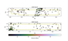 |
Fig. 1 KiDS footprints and galaxies between between 2 and 47 Mpc, taken from the galaxy group catalog of Kourkchi & Tully (2017). The symbols denote the galaxies and the color scale represents their distances based on the Hubble Lêmaitre law. The overdensity of galaxies in the center of the upper panel comprises the Virgo cluster and its surroundings, and the overdensity in the lower left of the lower panel is the Fornax cluster. The dashed yellow lines indicate the areas covered by the KiDS data. |
3 Object detection and initial selection
We aim to scan through the 1004 deg2 area visible in the KiDS images and detect the objects that can be reliably detected from the data. We used MTO (Teeninga et al. 2016) for the object detection; this is a max-tree based detection algorithm that allows for nesting of the objects and is highly nonparametric. As has been demonstrated by Haigh et al. (2021) and Venhola et al. (2022), MTO is more complete and precise in the detection of LSB galaxies than ProFound (Robotham et al. 2018), SExtractor (Bertin & Arnouts 1996), and NoiseChisel (Akhlaghi & Ichikawa 2015), which are the other commonly used object detection algorithms. Additionally, MTO is essentially free of parameters that significantly affect the detection efficiency, which makes it optimal for the detection of dwarf galaxies from this kind of large dataset. We performed the object detection in two parts: first we probed the detection completeness limits of the MTO on the KiDS images (Section 3.1) and then we applied MTO for the KiDS data and performed object selection (Section 3.2).
3.1 Detection completeness
We tested the detection completeness of MTO for the KiDS images by injecting artificial dwarf galaxies into the images. For this purpose, we created dwarf galaxies that are modeled with 2D Sérsic profiles. The injected galaxies were simulated on small postage stamp images with the pixel size matched with KiDS. The stellar light distribution of the simulated galaxy was first added to the central parts of the image. The image was then convolved with the r′-band PSF model (described in Section 2). Finally a Poisson distributed noise was simulated based on the ADU value of the data and the gain of the images. These simulated postage stamps were then added to the KiDS mosaics. We injected 100 dwarf galaxies per r′-band KiDS image to random positions and repeated the process 80 times, providing 8000 artificial galaxies with known structural parameters and locations. The parameters of the artificial galaxies were chosen randomly between the following ranges: 2 arcsec < Re <64 arcsec, 21.5 mag arcsec−2 < μ̄e′,r′ < 29 mag arcsec−2, 0.5 < Sérsic n <2, and 0.2 < b/a < 1. These properties for the simulated dwarfs are similar to the dwarfs found in the groups and clusters in the nearby Universe (see e.g., Venhola et al. 2018 and Poulain et al. 2021).
In order to test the completeness of our detection and selection algorithm, we then ran MTO for all the simulated fields. We did a similar selection for these simulations as we did for the real observations, which was based on the detected object size (effective radius based on detected pixels, Re,det > 3 arcsec) and surface brightness (median surface brightness of the detected pixels, μdet > 22 mag arcsec−2). The images also contain real objects, so it is crucial to ensure that the detections we obtain correspond to the simulated galaxies. In order to ensure that the detected objects correspond to the simulated galaxies, we first ran the detection for the KiDS image without the simulated galaxies and then with the simulated galaxies and removed the detections in both runs that were the same. For the criterion of detection of the simulated galaxy, we required the detection to be within 0.5Re of the object center.
We show the results for the detection completeness for the simulated galaxies as a function of their surface brightness and size in the upper panel of Fig. 2. We obtain complete detections with no bias in the object size down to 25 mag arcsec−2. After that limit the small objects tend not to be selected using our detection algorithm. For the analysis of the number of dwarfs in the groups, it is also significant to know the limiting magnitude of our catalog that is based on the detected objects. We show the detection completeness as a function of magnitude in the lower panel of Fig. 2. We find that our limiting magnitude is between 18 and 19 mag in the r′ band. We assume from now on that we have more than 75% completeness for objects brighter than 18 mag and with an effective radius larger than 5 arcsec.
To ensure that our detection algorithm and selection criteria do not introduce significant selection biases during the detection and selection, we also analyzed the parameters of the detected galaxies with regard to the flat input distributions. In Fig. 3 we show the trends for the b/a and Sérsic n of the detected galaxies as a function of their surface brightness. There is a slight trend for both parameters, so that for the faintest objects we preferably detect more peaked and round objects. This trend is expected since, when detecting objects near the noise limit of the data, both increasing n and increasing b/a (when keeping μ̄e,r′ fixed) increases the signal of the object.
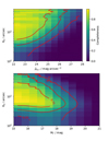 |
Fig. 2 Completeness based on our detections and selection limits. The upper panel shows the input effective radii and mean effective surface brightness in the r′ band for artificial galaxies embedded in the KiDS images. The lower panel shows the input r′-band magnitude and effective radii. The colors in the images indicate the fraction of detected and selected galaxies in a given parameter space and the red lines show the 25, 50, and 75% completeness contours. |
3.2 Detection and initial selection of objects
We then ran MTO for the 1004 KiDS fields. Our detection resulted 6.5 × 10⁷ initial detections, including dwarf galaxies, stars, imaging artifacts, and background objects (see Fig. 4). In order to limit our sample into nearby (d < 60 Mpc) resolved dwarf galaxies, we applied a selection cut in the mean effective surface brightness of the detected pixels, μ̄det,r′ > 22 mag arcsec−2, and the effective radius based on detected pixels, Re,det > 3 arcsec. This cut limits our sample to 9794 galaxies. We used the 3 arcsec size limit due to the fact that number of objects increases exponentially with a decreasing size limit, which quickly makes the sample size problematically large, and due to the fact that we want to be able to analyze the morphology of the selected objects. In Fig. 5, we show the distribution of detected objects’ detection magnitudes, sizes, and median surface brightnesses. We publish the parameters of the initial detections and galaxies selected based on their size and surface brightness in separate electronic catalogs with this paper (see Appendix A for details).
After selecting objects based on their size and surface brightness, we used colors to further narrow the selection to nearby dwarfs. We measured u,, g′, r′, and i′-band aperture magnitudes for all the galaxies using an aperture with 3 arcsec radius. We used the g′ - r′ colors to exclude objects that have colors that are too red for dwarf galaxies. We used the limiting color of g′ - r′ < 0.9. This color cut is relatively conservative as this color is typical for massive elliptical galaxies that have older and more metal-poor stellar populations than dwarfs. For example, in the Fornax cluster, where the majority of dwarfs are of early type, this color cut would not have excluded any dwarfs (see Venhola et al. 2018). We did not use color selection at the blue end of colors, since dwarf galaxies in the field are likely star-forming and metal-poor, and thus they can be very blue. Additionally, using color cuts at the blue end would likely not exclude any actual high-redshift background galaxies from the selection. Using the color selection, we are left with 6230 galaxies. We show the color distribution of the galaxies selected based on their sizes and surface brightness and the color selection limit used in Fig. 6.
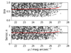 |
Fig. 3 Distribution of the axis ratios (upper panel) and Sérsic indices (lower panel) of the simulated dwarfs detected with MTO as a function of the mean effective surface brightness in the r″ band. The black and red lines show the input mean and output running mean of the parameter distribution, respectively. |
4 Photometric pipeline
After removing the objects that are unlikely to be dwarfs based on their surface brightness, color index, or size, we were left with 6230 objects. We performed photometric measurements for all these objects. We used GALFIT 3.0 (Peng et al. 2010) to fit Sérsic profiles to the 2D-light distribution of the galaxies. We used the same pipeline as Venhola et al. (2022), but for the sake of completeness we also briefly describe the main steps here.
At first, we cut thumbnail images of the science mosaics in all the available bands using the coordinates and sizes of the selected objects. In the cutting, we used the detection coordinates and cut the thumbnails at a distance of 10×Re,det. Similarly, we also cut the segmentation map image and the weight in the r′ band, which we then transformed into a σ image by taking an inverse value of the square root of each pixel’s value in the weight image. As is described in Section 2, we also generated a PSF model for each field that was used for the fitting process of the objects in the given field.
We then used the segmentation map and the corresponding object list to generate masks and input models for GALFIT. We selected the main object and the nearby bright stars and galaxies into the input model. They were fit with Sérsic functions within GALFIT. However, we limited the maximum number of objects in the model to five. In the case of more than five bright objects, we selected the brightest ones into the model and masked the others. All other sources in the image were masked using the MTO segmentation map. In GALFIT, we also fit the background of the image with a plane with three degrees of freedom (intensity level in the center and the gradients along the two axes).
We acknowledge that fitting all galaxies with single Sérsic profiles does not provide excellent models for all dwarfs, especially if they are distorted or star-forming irregulars. However, early-type low-mass dwarfs are generally mostly featureless (see Janz et al. 2016 and Su et al. 2021) and can thus be fairly robustly fit with Sérsic profiles. Star-forming dwarfs may have a more irregular and complicated structure that is not well fit by any analytical profile, but having the same type of measurements for them as for the early-type dwarfs makes the catalog uniform and easy to interpret.
We visually checked the fit quality of all the models modeled with GALFIT. Among the automatically fit objects, we found on the order of 300 galaxies for which the initial models were poor due to galaxies being fit with several Sérsic profiles instead of one or having some poorly masked neighboring galaxies in the images. In such cases, we corrected the input models, fixed the masks, and refit the galaxies until a proper fit was obtained.
As a result from the GALFIT models, we obtained for each galaxy the r′-band magnitude, axis ratio, position angle, Sérsic n, and effective radius. We then also measured aperture magnitudes within the r′-band Re for all dwarfs in the four optical bands, using the aperture ellipticity and position angle obtained from the GALFIT fits. Additionally, we measured the residual flux fractions (RFF, see Hoyos et al. 2011),
 (1)
(1)
where nr<Rp is the number of pixels within the Petrosian radius (RP) where the galaxy’s surface brightness is one fifth of the mean surface brightness within that radius. The term |datai -modeli| corresponds to the absolute value of residual flux at a given point, Fr<RP is the total flux within the RP, and σi is the pixel value of the sigma image. RFF can be used as a measure for the significance of the residuals after subtracting the Sérsic fit profile from the galaxy.
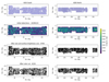 |
Fig. 4 Distribution of the data and detections on the sky. The top panel shows the available KiDS exposures. The second panel from the top shows the number density of detections (the corresponding color bar is shown on the right). The third panel from the top shows the objects selected based on their detection size and surface brightness. The bottom panel shows the distribution of the detections when the color selection is also applied. The numbers above the panels indicate the number of objects left when the corresponding selection criteria are applied. The various selection criteria are described in the main text. |
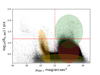 |
Fig. 5 Detection parameters of KiDS detections. The black symbols show the detection parameters of every 20th detection. The continuous and dashed red lines show the size and surface brightness selection limits, respectively. The colored ellipses indicate the major contributors to the different structures in the parameter space: the orange ellipse indicates an area mostly populated by saturated stars, the yellow ellipse corresponds to stars, green to nearby galaxies, and brown to higher-redshift galaxies. |
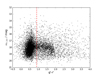 |
Fig. 6 Colors of size and SB selected objects. Black symbols show the g′ - r′ aperture colors and detection r′-band magnitudes for the objects selected based on their sizes and surface brightness. The dashed red line shows the selection limit adopted for the colors. |
5 Morphological object selection
For the removal of artifacts and the morphological classification of galaxies, we generated three-band color (rgb) images by combining the i′, r′, and g′-band KiDS thumbnail images for the red, green, and blue channels in the rgb images, respectively. For each galaxy, we generated a thumbnail image the size of 20 times the detection major axis centered on the detected galaxies. We then visually classified the objects into six categories:
Class 0 - artifacts: the detected object is either a stellar halo or some data reduction artifact that does not resemble a galaxy, or the data around the detected galaxy are partly missing, or it does have significant reduction defects.
Class 1 - dwarfs: objects that show a clear dwarf morphology, i.e., they do not show clear spiral arms or bulge or bar components and have low surface brightness.
Class 2 - likely dwarfs: objects that appear similar to dwarfs but have a slight disturbance or hint of structure, which may introduce a small possibility of interpreting their nature incorrectly.
Class 3 - possible dwarfs: objects for which the morphology is clumpy or there are some faint structures, which cannot be straightforwardly interpreted as spiral galaxy structures.
Class 4 - likely giant: galaxies that show separate bulge and disk components and may have faint spiral arms or a bar. Also, bright elliptical galaxies that have large diffuse outskirts and were selected due to the low mean surface brightness of detected pixels are classified in this category.
Class 5 - giant: galaxies that show a clear bulge and disk and well-defined spiral arms are classified in this category.
We classified all the 6230 galaxies selected based on their size, surface brightness, and colors according to this classification system. Examples of each morphological class are shown in Fig. 7. The distribution of number of objects in the different morphological groups is shown in Fig. 8. Out of 6230 objects, we classified 933 as possible dwarfs, 793 as likely dwarfs, and 763 as dwarfs. From now on we use the name dwarf candidates for the objects in these three classes. We show the distribution of dwarf candidates and dwarfs in Fig. B.1.
6 Results
In the last section, we described the method we used to derive the dwarf galaxy catalog containing 2489 dwarf candidates. We present a short description of the catalog and its contents in Appendix B and share the whole catalog in electronic format with the paper. Here we analyze the resulting catalog, by comparing it with other dwarf catalogs of the same areas, and analyze the number of dwarfs in groups and their spatial distributions within groups.
6.1 Purity and completeness based on archival data
In order to estimate the completeness and purity of our catalog, we compared it with the NASA/IPAC Extragalactic Database (NED1). We searched from NED for galaxies within 1 arcsec of the positions of the galaxies in our catalog. We found matches for 2961 galaxies in our catalog. We then compared the radial velocities of the matched objects with our object classifications. We show the results of that comparison in Fig. 9. It appears that for class 1 (galaxies that appear as dwarfs) the number of objects that do not have counterpart in NED is roughly 70% and that fraction decreases toward classes that contain galaxies that are less likely to be dwarfs. That can be easily explained by the fact that the objects in class 1 have typically a lower surface brightness, and thus fewer spectroscopic measurements. Also the relative fraction of objects that are spectroscopically confirmed to be in the nearby Universe is highest among class 1 and decreases monotonically toward higher class numbers. On the other hand, the fraction of spectroscopically confirmed background objects is lowest in class 1 and increases monotonically toward class 5. Thus, it seems that the morphological classification between local Universe dwarfs and background spirals seems to correlate well with the spectroscopic data.
In order to undertake a sanity check for completeness, we randomly selected two groups, namely NGC 4179 and IC 1125, and searched for spectroscopically confirmed and otherwise dwarf-like galaxies in those groups that are not in our catalog. We searched NED for objects within the virial radii of those groups and performed visual inspection of the KiDS images within the virial radius.
In the IC 1125 group, there are no other spectroscopically confirmed members than the main galaxy. We visually examined the area within the virial radius and the only potential dwarf-like object that we identified was identified in our catalog (KiDS_DR4.0_233.0_-1.5_5).
In case of NGC 4179, there were three spectroscopically confirmed group members in the NED: SDSS J121241.71+003910.5, SDSS J121337.44+010350.2, and DESI J183.3440+01.1247. All of them were in our initial detection lists, but only SDSS J121241.71+003910.5 is in our final catalog (KiDS_DR4.0_183.0_0.5_2), since the other ones had either too small an effective radius (DESI J183.3440+01.1247) or too bright a surface brightness (SDSS J121337.44+010350.2). We visually found a few additional dwarf candidates in that group that were initially detected by our algorithm, but were rejected from the final catalog based on their too small detected effective radius.
Based on these checks, we conclude that our detection and classification pipeline seems to work relatively robustly in terms of not missing significant amount of obvious dwarfs and there being a clear correlation between the morphological classifications and nature of the objects. However, as is seen from our tests, it appears that our size and surface brightness selection limits that we used in the initial selections exclude some bright and small dwarfs in the groups. This caveat should be taken into account when using the catalog for scientific analysis.
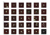 |
Fig. 7 Examples of galaxies belonging to the different morphological classes used in the classifications. From top to bottom, the rows show examples of dwarfs (class 1), likely dwarfs (class 2), possible dwarfs (class 3), likely giants (class 4), and clear giant galaxies (class 5), respectively. |
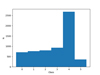 |
Fig. 8 Distribution of classified objects in the different morphological groups as described in Section 5 (examples of the members in the different classes are shown in Fig. 7). |
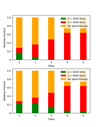 |
Fig. 9 Distribution of known recession velocities for the different morphological classes. The green, red, and orange bars show the relative fraction of objects that have radial velocities below the limit value, above the limit value, or no velocity measurement, respectively. We use velocity limits of 4500 and 9000 km s−1 in the upper and lower panels, respectively. |
6.2 Comparison with other catalogs
In order to quantitatively validate the quality of measured galaxy properties, we compared the obtained catalog with the available catalogs in the literature. We focused here mostly on the deep surveys done in the local Universe with comparable data to ours. For the Fornax cluster dwarf galaxies, we used the Venhola et al. (2018) and Venhola et al. (2022) galaxy catalogs, which are derived from the Fornax Deep Survey data (see Peletier et al. 2020). In order to increase the spatial coverage of this comparison we also used the Mass Assembly of early-Type gaLAxies with their fine Structures dwarf galaxy catalog (MATLAS, Poulain et al. 2021). The MATLAS catalog contains 2210 dwarfs in various nearby groups that contain early-type galaxies.
We compared the r′-band magnitudes, effective radii, and Sérsic indices of our catalog and the above mentioned catalogs in the literature. There are 33 galaxies common between this work and the FDSDC. We show the comparison between the structural properties of our sample and the FDSDC in Fig. 10 with the black symbols. We find that the magnitudes in the two works match very accurately, but the effective radii measured in this work are systematically slightly smaller than in the FDS and MATLAS and there is quite a large scatter in the obtained Sérsic indices with regard to other catalogs. The difference in the sizes is likely related to the differences in the background subtraction of the datasets. For MATLAS and FDS, the background subtraction is done by stacking the science images to produce a master background, which is then subtracted from the images, whereas KiDS uses filtering of the background that can lead to oversubtraction of the outer parts of the galaxies. We thus acknowledge that the sizes of the galaxies in our catalog may be slightly underestimated due to the data processing techniques used in KiDS and they should not be used for detailed structural analysis.
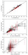 |
Fig. 10 Structural parameters of the galaxies in our catalog compared to their parameters based on the FDS (black symbols, Venhola et al. 2018 and Venhola et al. 2022) and MATLAS (red symbols, Poulain et al. 2021). The panels show the comparison for apparent magnitude (top panel), effective radii (middle panel), and Sérsic indices (bottom panel). Error bars in the different panels indicate the measurement uncertainties of the parameters. For the MATLAS dwarfs, we do not show the uncertainties as they were not present in the catalog. |
6.3 Environment of the objects
In order to estimate the associations of dwarfs with different galaxy groups, we used the catalog of Kourkchi & Tully (2017). We first identified the galaxy groups in the catalog within 60 Mpc that are covered by the KiDS data. We identified 26 fully covered (coverage >90% of the R200) galaxy groups and 12 partially covered (coverage <90%) within the survey area. These groups and their properties are listed in Table E.1. We then associated the dwarfs with morphological classes 1, 2, and 3 that lie within the R200 of those galaxy groups as dwarf galaxies associated with those groups. Based on this analysis, 408 dwarf candidates in our sample are in a group environment and 1859 dwarfs lie outside of groups. The possible associations of dwarfs with groups are listed in Table B.1.
Since there is uncertainty in the morphological classifications of dwarfs and their distances, we also estimated the bias correction for the number of dwarfs in the groups. We selected dwarfs that are not associated with any group based on the Kourchi & Tully group catalog and calculated the mean surface number density of dwarfs outside of the groups by dividing the number of dwarfs outside the groups by the area of the observations that is outside of the projected R200 of the identified groups. We obtained an average surface number density of dwarfs outside the groups of 1.8 dwarfs per deg2. The corresponding dwarf number density within the groups is 4.9 dwarfs per deg2.
6.4 Number of dwarfs in groups
We aim to investigate the number of objects in the different groups as a function of the group mass. However, there are two biases that need to be taken into account while doing that. Firstly, the groups are located at different distances, which might affect the completeness limits of our observations in these groups. Secondly, there might be misclassified objects within the groups, or objects that are only overlapping with the group by projections and that are not really associated with the group.
We first estimated the completeness at various distances by comparing the magnitude completeness limits at the various distances with the distribution of the magnitudes of the galaxies associated with various groups. We show the distance-corrected absolute magnitude selection limits with the absolute magnitude distribution of the objects in various groups (assuming that the dwarfs projected within the groups Rvir are at the distance of the group) in the upper panel of the Fig. 11. Optimally, we want to compare the number of dwarfs in the groups by comparing the numbers in the same complete mass range. We thus identified the completeness limit of the furthermost group in our data (completeness limit mr =19.5 mag corresponds to Mr′ ≈ −14 mag at the distance of 58 Mpc) and transformed that apparent magnitude into stellar mass using the transformation by Taylor et al. (2011) (similarly as Venhola et al. 2019):
 (2)
(2)
where g′, r′, and i′ are the aperture magnitudes in the corresponding bands and Mr′ is the absolute magnitude in the r′ band (assuming the distance to be the same as the associated group’s distance). Transforming the completeness limit to stellar mass, using the typical dwarf colors, we find that as an order-of-magnitude estimate, the limit corresponds to a stellar mass of  , which we adopt as our mass limit in the following analyses.
We show the distribution of stellar masses for dwarf candidates in the various groups and the mass selection limit corresponding to the mass of the faintest dwarf in the furthest group in the lower panel of Fig. 11. We excluded dwarfs that have masses below our mass selection limits from the further analysis in order to make a fair comparison.
We then calculated the number of dwarfs that are located within the R200 of each group. We also estimated the upper and lower limits of the number of dwarfs by scaling the number of dwarfs with a fraction of covered area of each group’s R200 and by subtracting the number of dwarfs that is expected to be appearing as group members only due to projection effects, i.e., by multiplying the area closed by the group’s R200 and multiplying that by the mean number density of dwarfs outside the groups (see Section 6.2). We also did the same analysis by using only the morphological classes 1 and 2 and also including objects with class 3. In this analysis, we excluded two groups where the completeness is below 20% because the number of dwarfs in them is highly uncertain. The results of this analysis are shown in Fig. 12.
We find that the number of dwarfs scales with the groups’ mass in a log-linear manner. There is very little difference for the general trend when different morphological selection limits or corrections are used.
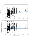 |
Fig. 11 Distribution of the absolute magnitudes (upper panel) and stellar masses (lower panel) of the dwarf candidates as a function of the associated groups’ distance. The blue lines in the upper and lower panels show the completeness limit of the detections and the stellar mass limit used, respectively. |
6.5 Spatial distribution of dwarfs in groups
Another interesting factor to consider is whether the distribution of dwarfs in the groups is isotropic. For that analysis, we selected only the groups that have more than 90% areal coverage. We calculated the axis ratios of the distribution of dwarf candidates within the groups by calculating the second-order moments of the dwarf distribution within the selected groups as follows:
 (3)
(3)
 (4)
(4)
 (5)
(5)
 (6)
(6)
 (7)
(7)
where x and y are the group-centric distances along the right ascension and declination axes, N is the number of dwarfs in the given group, and a and b are the group’s major and minor axes, respectively.
We also identify a possible correlation with the axis ratio of the group and its virial mass. We tested the correlation with Pearson’s correlation test for three samples containing the given morphological classes (inside the brackets): sample 1: [1], sample 2: [1,2], and sample 3: [1,2,3] and ran the test for galaxies projected within the virial radii and within two virial radii. We show the group shape analysis for sample 1 in Fig. 13 and show similar plots for the samples 2 and 3 in Figs. C.1 and C.2, respectively. For the dwarf within one virial radius of the group we find a Pearson’s correlation coefficient of c=0.52, 0.42, 0.42 for samples 1, 2, and 3, respectively, with p values for noncorrelation being p=0.12, 0.15, and 0.15, respectively. For the dwarfs within two virial radii, the statistics are c=0.46, 0.30, and 0.21, with p values of p=0.08, 0.24, and 0.39 for samples 1, 2, and 3, respectively. Thus, we find that the correlations are not statistically significant.
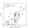 |
Fig. 12 Number of dwarf candidates as a function of group’s mass. The black and red symbols show the number of candidates with morphological classes less or equal to 2 and 3, respectively. The black error bars show the uncertainty of the numbers: we obtained lower limits by estimating number of the objects whose projected locations are likely overlapping with the group by chance and the upper limits by extrapolating the number of dwarfs for the whole Rvir area in case of partially covered groups. The green line shows the linear fit to the data. |
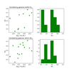 |
Fig. 13 Shapes of the dwarf galaxy distribution in the KiDS groups for galaxies that are morphologically certainly dwarfs. In the left panels, we show the axis ratios of the groups as a function of the group’s virial mass. In the right panels, we show the distribution of the axis ratios for the groups. The upper panels show the distributions for the dwarfs within the virial radii and the lower panels show the same figures for dwarfs within two virial radii. The other selection criteria used for the analysis are described in the main text. |
7 Discussion
In this work, we have produced a dwarf galaxy candidate catalog that contains dwarfs in various galactic environments, which provides an interesting dataset with which to study the effects of the environment of the dwarf populations. However, to obtain full certainty about the candidate galaxies’ distances, spectroscopic follow-ups are needed. Currently we do not have the distances, which restricts us from performing a detailed structural analysis of galaxies in the various environments. However, it is nevertheless interesting to compare some general properties of the candidate populations with the state-of-art cosmological simulations, while trying to control the possible biases caused by the distance uncertainties.
7.1 Comparison of dwarf numbers with Illustris-TNG
We compared our observed relation between the number of dwarf and group mass with the corresponding relation found in the Illustris-TNG hydrodynamical simulation. In order to make a fair comparison, we took into account the numerical accuracy of the simulations and applied similar selection methods for the galaxies as were applied with the catalog based on the KiDS observations.
For the comparison, we used the publicly available Illustris-TNG TNG50-1 simulation, which has the highest resolution of the publicly available Illustris-TNG simulations. For TNG-50-1, the simulation particle sizes are for baryons Mbar = 5.7 × 10⁴ M⊙ and for DM particles MDM = 3.1 × 10⁵ M⊙. This means that for a dwarf with a stellar mass of 107 M⊙ (corresponding to our completeness limits), the dwarf is simulated with at least 200 baryonic particles. This is not sufficient to accurately simulate the structural properties of such dwarfs (especially when considering the gravitational softening which is close to the effective radii of these dwarfs), but we assume that the total content of the baryonic matter is at the right order of magnitude.
The halo catalogs of the Illustris-TNG contain the photometric properties of the simulated galaxies. We used the g′, r′, and i′ colors and r′-band absolute magnitudes listed in the halo catalog to estimate the stellar masses of the simulated dwarfs similarly as we did for the KiDS dwarf candidates. We show the comparison between the baryonic mass and the photometrically estimated stellar mass for all the dwarf galaxies between stellar mass 7 <  < 9.5 for the Illustris-TNG galaxies in the upper panel of Fig. 14. The agreement between the stellar mass and the photometrically estimated stellar mass is very good for most objects. Some scatter can be seen in the range of
  = 8-10, which is introduced by the gas-rich dwarf galaxies.
We then selected dwarfs with stellar mass 7 <  < 9.5 from the IllutrisTNG-50 simulation and counted the number of dwarfs within R200 in the simulated groups. We show the numbers as a function of the group mass in the lower panel of Fig. 14. We find a very similar log-linear trend between the illustrisTNG group mass and number of dwarfs as found for the KiDS groups.
We then compared the number of dwarfs found in the simulation and in the KiDS data as a function of the groups’ mass. We compared dwarfs with stellar mass 7 <  < 9.5 in KiDS and IllustrisTNG. In the KiDS dataset, we selected dwarf candidates with class < 3 and corrected the number of dwarfs in each group by dividing the number by the coverage factor and subtracted the number of dwarfs that are expected to overlap with the group due to projection effects. We show the results of this comparison in Fig. 15. We find that the fits match well between the simulations and the KiDS groups. However, in the observational data the scatter of individual points around the trend is much larger than in the simulations. It is difficult to obtain certainty with the dataset at hand whether the difference in the scatter is due to the observational biases in the dataset or whether it is a sign of some fundamental difference between the observed and simulated groups.
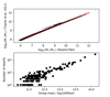 |
Fig. 14 Photometrically estimated stellar mass versus the baryonic mass for the IllustrisTNG dwarfs (upper panel) and the number of dwarfs within R200 as a function of group total mass (lower panel) in IllustrisTNG-50 simulation. |
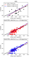 |
Fig. 15 Comparison of group mass-dwarf number relation between KiDS and IllustrisTNG50 groups. |
7.2 Comparison of group shapes with IllustrisTNG
We also compared the shapes of the groups in the KiDS and IllustrisTNG datasets. For KiDS dwarfs, we analyzed the dwarf candidates with different morphological classes in three different samples (similarly to in Section 6.5) within the R200 of the groups. We then calculated the flattening as described in Section 6.5. For the simulated groups, we selected dwarfs that are within the R200 of the group and have a stellar mass within the range of 7 <  < 9.5. We then calculated the flattening of the simulated groups similarly to how did it for the KiDS galaxies, but instead of the RA and Dec coordinates, we use the group-centric x and y coordinates (in kiloparsecs) in the simulation.
We show the distribution of the group shapes and the cumulative distributions in Figs. 16, C.3, and C.4. We test the similarity of the axis-ratio distributions in with the Kolmogorov-Smirnov test and found that the probability of them being drawn from the same intrinsic distribution are the following: sample 1: p = 0.78 , sample 2: p = 0.83, and sample 3: p = 0.32. Therefore, we do not find there to be a statistically significant difference between the KiDS and Illustris-TNG distributions. We also investigated how the number of dwarfs in the groups affects the flattening. We show the number of dwarfs versus flattening for both datasets in Fig. D.1.
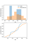 |
Fig. 16 Shape distribution of the groups based on their dwarf galaxies’ IllustrisTNG and KiDS dwarf candidates, when selecting objects from morphological class 1. The upper panel show the histograms of the normalized counts in both samples and the lower panel show the cumulative distributions. |
8 Summary and conclusions
In this work, we present a search for dwarf galaxies in the wide-field KiDS survey, which covers over 1000 deg2 in the u g ri bands. For that purpose, we used MTObjects, a software package that is optimal for detecting low-surface-brightness objects. Our initial detection over the whole survey included up to 7 × 10⁷ objects, including stars, galaxies, cirrus, and artifacts. Basic photometric parameters come from MTObjects itself. To get a handle on the color, we further applied aperture photometry in a small area in all bands. To reduce this immense catalog of detections, we applied stringent quality cuts in surface brightness, size, and color. These cuts limited the sample to 6230 objects. On these objects, we applied accurate photometry with GAL-FIT. The objects were then classified by eye in a six-step scheme, ranging from certain dwarf galaxy to certain giant galaxy. We find a total of 2489 likely dwarf galaxies. As a caveat: while we call them dwarf galaxies, they must be considered dwarf galaxy candidates until their distance is accurately established. To test our detection efficiency, we injected artificial dwarf galaxies randomly into each image. We fully detect artificial dwarf galaxies down to 25 mag arcsec−2, which sets the completeness limit of our survey.
To associate dwarf galaxies with their environments, we used the group catalog of Kourkchi & Tully (2017) and selected galaxy groups within 60 Mpc. We identified 26 groups in our footprint, and an additional 12 groups that are partially covered. For each group, we associated our dwarf galaxies if they reside within the virial radius of the host galaxy. Out of the 2489 dwarf galaxies in our sample, 408 reside in one of these group environments. The number of dwarfs in a group ranges from 1 to 129. We find a mean density of 4.9 dwarfs per deg2 in group environment, and 1.8 dwarfs per deg2 in the field.
Because the groups reside at distances between 10 and 60 Mpc, the completeness of our survey is a function of distance. From our artificial dwarf galaxy experiment, we can derive the completeness limits at various distances. We find a stellar mass of 107 M⊙ as our completeness threshold (while the faintest dwarf has a stellar mass of 105 M⊙).
With these dwarf galaxy catalogs, we conducted some comparisons to cosmological simulations; namely, the TNG50 box from the Illustris-YNG simulations. We were interested in two properties of the dwarf galaxy population: the number of dwarf galaxies per host and the overall shape of the dwarf galaxy population. We selected groups from TNG50 in the same stellar mass range as our observed groups. As a limit, we set 107 M⊙ to select dwarf galaxies. At this mass range, dwarf galaxies in TNG50 have at least 200 baryonic particles.
Comparing the number of dwarf galaxies in observed and simulated groups, we find similar trends. Fitting the number of dwarf galaxies as a function of group mass in TNG50, we find a power law. The KiDS groups follow a very similar power law, but have a larger scatter around the trend. This may be due to observational biases and incompleteness in our survey. When dwarf galaxies are hidden behind bright stars or extended objects, they cannot be detected even if they are above the completeness limit. On the other hand, the membership of the observed objects is not yet established and can be interpreted as upper limit. The MATLAS survey discovered over 2000 dwarf galaxy candidates (Habas et al. 2020; Poulain et al. 2021). Follow-up observations of 56 of their candidates with spectroscopy revealed that ~25% of the candidates were background objects (Heesters et al. 2023). If this is the case here as well, the observed trend would move further away from the predictions from TNG50. There would be too few observed dwarf galaxies. This is interesting, because for the MATLAS survey the opposite was proposed, also based on comparisons to TNG50; namely, that there are too-many observed dwarf galaxies or not enough simulated ones (Kanehisa et al. 2024). However, there are some key differences between these studies. MATLAS is a deeper, targeted survey, which employed a one-pointing strategy centered on early-type galaxies. This resulted in a very low surface brightness limit (28 mag arcsec−2) that, however, did not cover the full extent of the satellite system. With KiDS, we are not as deep (25 mag arcsec−2 ), but can cover the full radius of the satellite system. Here, with KiDS, we have both early-type and late-type galaxies, while MATLAS is limited to early-types.
Most of the dwarf galaxies around the Milky Way are arranged in a planar configuration (Pawlowski 2018) and such features were observed in other galaxy groups as well (e.g., Tully 2015; Heesters et al. 2021; Karachentsev & Kroupa 2024). This begs the question of whether we also find such structures around the giant galaxies in the footprint of KiDS. For that purpose we have measured the second moments of the satellite distribution and compared it to TNG50. The general distribution of group axis ratios, and thus the flattening distributions between the two samples, does not show a statistically significant difference. There are some caveats to consider. A second moment analysis takes into account the whole satellite population and is prone to outliers. However, not all dwarf galaxies must reside in a plane. This is, for example, the case for the Andromeda galaxy, where only half the satellites are in a thin, coherently moving plane (Ibata et al. 2013; Sohn et al. 2020). Such features are not picked up by our analysis. There are dedicated methods to detect such substructures (Heesters et al. 2021) but they need an analysis that is beyond the scope of this paper. Another caveat is that we did not consider the detailed environments for both the simulated and observed systems. For example, a system of two giant galaxies may naturally have a different flattening of satellites than an isolated system. This needs to be taken into account in further statistical studies of the spatial distribution of satellites.
With current and upcoming wide-field surveys, we are moving into a statistics-driven era in the study of dwarf galaxies. This brings new opportunities but also challenges to overcome. One of the first steps is being able to detect dwarf galaxies in such data in an automated fashion. Here, we have shown how to use dedicated software to detect faint sources, make quality cuts to reduce the number of false positives, and assess the detections by experts to get a pure dwarf galaxy sample. We have also shown how such dwarf galaxy catalogs can be used to test cosmology with whole populations of dwarf galaxy systems. The next step will be to assess these in more detail.
Data availability
The full Tables A.1 and B.1 are available at the CDS via https://cdsarc.cds.unistra.fr/viz-bin/cat/J/A+A/705/A78
Acknowledgements
We thank the referee for the constructive report, which helped to clarify and improve the manuscript. O.M. is grateful to the Swiss National Science Foundation for financial support under the grant number PZ00P2_202104. A.V. acknowledges funding from the Academy of Finland grant n:o 347089. We thank FINCA for the mobility grants that have been used for the research visits during the writing of this paper.
References
- Abbott, T. M. C., Adamów, M., Aguena, M., et al. 2021, ApJS, 255, 20 [NASA ADS] [CrossRef] [Google Scholar]
- Akhlaghi, M. 2019, arXiv e-prints [arXiv:1909.11230] [Google Scholar]
- Akhlaghi, M., & Ichikawa, T. 2015, ApJS, 220, 1 [Google Scholar]
- Bertin, E., & Arnouts, S. 1996, A&AS, 117, 393 [NASA ADS] [CrossRef] [EDP Sciences] [Google Scholar]
- Binggeli, B. 1994, European Southern Observatory Conference and Workshop Proceedings, 49, 13 [Google Scholar]
- Binggeli, B., Sandage, A., & Tammann, G. A. 1985, AJ, 90, 1681 [Google Scholar]
- Bradley, L., Sipőcz, B., Robitaille, T., et al. 2024, https://doi.org/10.5281/zenodo.12585239 [Google Scholar]
- Bullock, J. S., & Boylan-Kolchin, M. 2017, ARA&A, 55, 343 [Google Scholar]
- Carlsten, S. G., Greene, J. E., Peter, A. H. G., Beaton, R. L., & Greco, J. P. 2021, ApJ, 908, 109 [NASA ADS] [CrossRef] [Google Scholar]
- Chambers, K. C., Magnier, E. A., Metcalfe, N., et al. 2016, arXiv e-prints [arXiv:1612.05560] [Google Scholar]
- Chiboucas, K., Karachentsev, I. D., & Tully, R. B. 2009, AJ, 137, 3009 [Google Scholar]
- Cote, S., Freeman, K. C., Carignan, C., & Quinn, P. J. 1997, AJ, 114, 1313 [CrossRef] [Google Scholar]
- Crosby, E., Jerjen, H., Müller, O., et al. 2023, MNRAS, 521, 4009 [Google Scholar]
- Crosby, E., Jerjen, H., Müller, O., et al. 2024, MNRAS, 527, 9118 [Google Scholar]
- Danieli, S., Greene, J. E., Carlsten, S., et al. 2023, ApJ, 956, 6 [Google Scholar]
- de Jong, J. T. A., Verdoes Kleijn, G. A., Kuijken, K. H., & Valentijn, E. A. 2013, Exp. Astron., 35, 25 [Google Scholar]
- de Jong, J. T. A., Verdoes Kleijn, G. A., Erben, T., et al. 2017, A&A, 604, A134 [NASA ADS] [CrossRef] [EDP Sciences] [Google Scholar]
- Greco, J. P., Greene, J. E., Strauss, M. A., et al. 2018, ApJ, 857, 104 [NASA ADS] [CrossRef] [Google Scholar]
- Habas, R., Marleau, F. R., Duc, P.-A., et al. 2020, MNRAS, 491, 1901 [NASA ADS] [Google Scholar]
- Haigh, C., Chamba, N., Venhola, A., et al. 2021, A&A, 645, A107 [NASA ADS] [CrossRef] [EDP Sciences] [Google Scholar]
- Heesters, N., Habas, R., Marleau, F. R., et al. 2021, A&A, 654, A161 [NASA ADS] [CrossRef] [EDP Sciences] [Google Scholar]
- Heesters, N., Müller, O., Marleau, F. R., et al. 2023, A&A, 676, A33 [NASA ADS] [CrossRef] [EDP Sciences] [Google Scholar]
- Heesters, N., Chemaly, D., Müller, O., et al. 2025, A&A, 699, A232 [NASA ADS] [CrossRef] [EDP Sciences] [Google Scholar]
- Hodge, P. W. 1971, ARA&A, 9, 35 [Google Scholar]
- Hoyos, C., den Brok, M., Verdoes Kleijn, G., et al. 2011, MNRAS, 411, 2439 [Google Scholar]
- Ibata, R. A., Lewis, G. F., Conn, A. R., et al. 2013, Nature, 493, 62 [NASA ADS] [CrossRef] [Google Scholar]
- Ibata, R. A., Ibata, N. G., Lewis, G. F., et al. 2014, ApJ, 784, L6 [NASA ADS] [CrossRef] [Google Scholar]
- Janz, J., Laurikainen, E., Laine, J., Salo, H., & Lisker, T. 2016, MNRAS, 461, L82 [Google Scholar]
- Kanehisa, K. J., Pawlowski, M. S., Heesters, N., & Müller, O. 2024, A&A, 686, A280 [NASA ADS] [CrossRef] [EDP Sciences] [Google Scholar]
- Karachentsev, I. D., & Kroupa, P. 2024, MNRAS, 528, 2805 [NASA ADS] [CrossRef] [Google Scholar]
- Karachentsev, I. D., Sharina, M. E., & Huchtmeier, W. K. 2000, A&A, 362, 544 [NASA ADS] [Google Scholar]
- Koposov, S., Belokurov, V., Evans, N. W., et al. 2008, ApJ, 686, 279 [NASA ADS] [CrossRef] [Google Scholar]
- Kourkchi, E., & Tully, R. B. 2017, ApJ, 843, 16 [NASA ADS] [CrossRef] [Google Scholar]
- Kroupa, P. 2012, PASA, 29, 395 [NASA ADS] [CrossRef] [Google Scholar]
- Kuijken, K., Heymans, C., Dvornik, A., et al. 2019, A&A, 625, A2 [NASA ADS] [CrossRef] [EDP Sciences] [Google Scholar]
- Mao, Y.-Y., Geha, M., Wechsler, R. H., et al. 2021, ApJ, 907, 85 [NASA ADS] [CrossRef] [Google Scholar]
- Müller, O., & Jerjen, H. 2020, A&A, 644, A91 [NASA ADS] [CrossRef] [EDP Sciences] [Google Scholar]
- Müller, O., & Schnider, E. 2021, Open J. Astrophys., 4, 3 [Google Scholar]
- Müller, O., Jerjen, H., & Binggeli, B. 2018, A&A, 615, A105 [Google Scholar]
- Nelson, D., Springel, V., Pillepich, A., et al. 2019, Comput. Astrophys. Cosmol., 6, 2 [Google Scholar]
- Pak, M., Rey, S.-C., Lisker, T., et al. 2014, MNRAS, 445, 630 [Google Scholar]
- Paudel, S., Yoon, S.-J., Yoo, J., et al. 2023, ApJS, 265, 57 [NASA ADS] [CrossRef] [Google Scholar]
- Pawlowski, M. S. 2018, Mod. Phys. Lett. A, 33, 1830004 [NASA ADS] [CrossRef] [Google Scholar]
- Pawlowski, M. S., Müller, O., Taibi, S., et al. 2024, A&A, 688, A153 [NASA ADS] [CrossRef] [EDP Sciences] [Google Scholar]
- Peletier, R., Iodice, E., Venhola, A., et al. 2020, ArXiv e-prints [arXiv:2008.12633] [Google Scholar]
- Peng, C. Y., Ho, L. C., Impey, C. D., & Rix, H.-W. 2010, AJ, 139, 2097 [Google Scholar]
- Poulain, M., Marleau, F. R., Habas, R., et al. 2021, MNRAS, 506, 5494 [NASA ADS] [CrossRef] [Google Scholar]
- Revaz, Y., & Jablonka, P. 2018, A&A, 616, A96 [NASA ADS] [CrossRef] [EDP Sciences] [Google Scholar]
- Robotham, A. S. G., Davies, L. J. M., Driver, S. P., et al. 2018, MNRAS, 476, 3137 [NASA ADS] [CrossRef] [Google Scholar]
- Sales, L. V., Wetzel, A., & Fattahi, A. 2022, Nat. Astron., 6, 897 [NASA ADS] [CrossRef] [Google Scholar]
- Sawala, T., Cautun, M., Frenk, C., et al. 2023, Nat. Astron., 7, 481 [Google Scholar]
- Smercina, A., Bell, E. F., Price, P. A., et al. 2018, ApJ, 863, 152 [NASA ADS] [CrossRef] [Google Scholar]
- Sohn, S. T., Patel, E., Fardal, M. A., et al. 2020, ApJ, 901, 43 [NASA ADS] [CrossRef] [Google Scholar]
- Springel, V., Wang, J., Vogelsberger, M., et al. 2008, MNRAS, 391, 1685 [Google Scholar]
- Su, A. H., Salo, H., Janz, J., et al. 2021, A&A, 647, A100 [EDP Sciences] [Google Scholar]
- Tanoglidis, D., Drlica-Wagner, A., Wei, K., et al. 2021, ApJS, 252, 18 [Google Scholar]
- Taylor, E. N., Hopkins, A. M., Baldry, I. K., et al. 2011, MNRAS, 418, 1587 [Google Scholar]
- Teeninga, P., Moschini, U. C., Trager, S., & Wilkinson, M. 2016, Mathematical Morphology - Theory and Applications (Hoboken: Wiley), 1 [Google Scholar]
- Tully, R. B. 2015, AJ, 149, 54 [NASA ADS] [CrossRef] [Google Scholar]
- Venhola, A., Peletier, R., Laurikainen, E., et al. 2018, A&A, 620, A165 [NASA ADS] [CrossRef] [EDP Sciences] [Google Scholar]
- Venhola, A., Peletier, R., Laurikainen, E., et al. 2019, A&A, 625, A143 [EDP Sciences] [Google Scholar]
- Venhola, A., Peletier, R. F., Salo, H., et al. 2022, A&A, 662, A43 [NASA ADS] [CrossRef] [EDP Sciences] [Google Scholar]
The NASA/IPAC Extragalactic Database (NED) is operated by the Jet Propulsion Laboratory, California Institute of Technology, under contract with the National Aeronautics and Space Administration. Url: https://ned.ipac.caltech.edu/
Appendix A Detection catalogs
We show here a short example of the detection catalog. The complete catalog is published as an additional electronic material with this paper. The contents of the catalog are described in Table A.1.
Section of catalog of the initial detections.
Appendix B Catalog of dwarf candidates
In Sections 3, 4, and 5, we described the production of dwarf galaxy catalog of the KiDS data. The full catalog is available as an electronic version accompanying this paper. In Table B.1, we show a part of the catalog as an example. The catalog contains the following columns:
ID - Running identification number for the galaxy.
R.A. - Right ascension coordinate of the galaxy in ICRS coordinates using degrees.
Dec. - Declination coordinate of the galaxy in ICRS coordinates using degrees.
mr′ - r′-band apparent magnitude of the galaxy obtained from GALFIT Sérsic fit.
Re - Effective radius of the galaxy in arcsec obtained from GALFIT Sérsic fit.
Sérsic n - Sérsic index of galaxy obtained from the GALFIT Sérsic fit.
b/a - Minor-to-major axis-ratio obtained from the GALFIT Sérsic profile fit.
u′/g′/r′/i′ - Aperture magnitude obtained with elliptical aperture within the Re in a given band. If any band is missing, we filled −1 for the value.
RFF - Residual flux fraction as defined in Equation 1.
likely group - If galaxy’s projected position is within the virial radius from some group from Kourkchi & Tully (2017), we list the name of the group here. If galaxy does not reside within the virial radius of any group, the catalog value is set to None.
Class - morphological classification of the object based on our morphological analysis described in Section 5.
A section of the dwarf catalog generated from the data of KiDS.
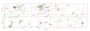 |
Fig. B.1 Locations of the dwarf candidates in this work with the known groups in the nearby Universe. The black, gray, and red symbols show the locations of the dwarfs, likely dwarfs and possible dwarfs. The green circles show the R200s of the groups from Kourkchi & Tully (2017) with the group’s central galaxy shown with the red text in the center of the corresponding group. |
Appendix C Group shapes
We show in Fig. C.1 and Fig. C.2 the similar shape analysis as in Fig. 13, but using the morphological types [1,2] (sample 2) and [1,2,3] (sample 3), respectively. For completeness we show also the group shape comparisons between KiDS and Illustris-TNG for the sample 2 and sample 3 in Fig. C.3 and Fig. C.4.
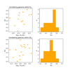 |
Fig. C.1 Same as Fig. 13, but the shapes are shown based on galaxies with mophological classification either 1 or 2. |
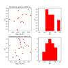 |
Fig. C.2 Same as Fig. 13, but the shapes are shown based on galaxies with mophological classification either 1, 2, or 3. |
Appendix D Shapes as a function of dwarf number
We analyzed how the shapes of the groups in the KiDS and Illustris-TNG data are dependent on the number of the dwarfs. The distributions as a function of groups’ dwarf abundance are shown in Fig. D.1. We find that in general the groups become more round when the number of dwarfs increases and the trends are very similar for simulations and real data.
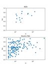 |
Fig. D.1 Shapes of the groups as a function of number of dwarfs. The panels show the distributions in KiDS (upper panel) and in IllustrisTNG (lower panel) data. |
Appendix E List of groups
In Table E.1, we present the groups from Kourkchi & Tully (2017) that overlap with the KiDS data.
List of groups covered by the KiDS data.
All Tables
All Figures
|
Fig. 1 KiDS footprints and galaxies between between 2 and 47 Mpc, taken from the galaxy group catalog of Kourkchi & Tully (2017). The symbols denote the galaxies and the color scale represents their distances based on the Hubble Lêmaitre law. The overdensity of galaxies in the center of the upper panel comprises the Virgo cluster and its surroundings, and the overdensity in the lower left of the lower panel is the Fornax cluster. The dashed yellow lines indicate the areas covered by the KiDS data. |
| In the text | |
|
Fig. 2 Completeness based on our detections and selection limits. The upper panel shows the input effective radii and mean effective surface brightness in the r′ band for artificial galaxies embedded in the KiDS images. The lower panel shows the input r′-band magnitude and effective radii. The colors in the images indicate the fraction of detected and selected galaxies in a given parameter space and the red lines show the 25, 50, and 75% completeness contours. |
| In the text | |
|
Fig. 3 Distribution of the axis ratios (upper panel) and Sérsic indices (lower panel) of the simulated dwarfs detected with MTO as a function of the mean effective surface brightness in the r″ band. The black and red lines show the input mean and output running mean of the parameter distribution, respectively. |
| In the text | |
|
Fig. 4 Distribution of the data and detections on the sky. The top panel shows the available KiDS exposures. The second panel from the top shows the number density of detections (the corresponding color bar is shown on the right). The third panel from the top shows the objects selected based on their detection size and surface brightness. The bottom panel shows the distribution of the detections when the color selection is also applied. The numbers above the panels indicate the number of objects left when the corresponding selection criteria are applied. The various selection criteria are described in the main text. |
| In the text | |
|
Fig. 5 Detection parameters of KiDS detections. The black symbols show the detection parameters of every 20th detection. The continuous and dashed red lines show the size and surface brightness selection limits, respectively. The colored ellipses indicate the major contributors to the different structures in the parameter space: the orange ellipse indicates an area mostly populated by saturated stars, the yellow ellipse corresponds to stars, green to nearby galaxies, and brown to higher-redshift galaxies. |
| In the text | |
|
Fig. 6 Colors of size and SB selected objects. Black symbols show the g′ - r′ aperture colors and detection r′-band magnitudes for the objects selected based on their sizes and surface brightness. The dashed red line shows the selection limit adopted for the colors. |
| In the text | |
|
Fig. 7 Examples of galaxies belonging to the different morphological classes used in the classifications. From top to bottom, the rows show examples of dwarfs (class 1), likely dwarfs (class 2), possible dwarfs (class 3), likely giants (class 4), and clear giant galaxies (class 5), respectively. |
| In the text | |
|
Fig. 8 Distribution of classified objects in the different morphological groups as described in Section 5 (examples of the members in the different classes are shown in Fig. 7). |
| In the text | |
|
Fig. 9 Distribution of known recession velocities for the different morphological classes. The green, red, and orange bars show the relative fraction of objects that have radial velocities below the limit value, above the limit value, or no velocity measurement, respectively. We use velocity limits of 4500 and 9000 km s−1 in the upper and lower panels, respectively. |
| In the text | |
|
Fig. 10 Structural parameters of the galaxies in our catalog compared to their parameters based on the FDS (black symbols, Venhola et al. 2018 and Venhola et al. 2022) and MATLAS (red symbols, Poulain et al. 2021). The panels show the comparison for apparent magnitude (top panel), effective radii (middle panel), and Sérsic indices (bottom panel). Error bars in the different panels indicate the measurement uncertainties of the parameters. For the MATLAS dwarfs, we do not show the uncertainties as they were not present in the catalog. |
| In the text | |
|
Fig. 11 Distribution of the absolute magnitudes (upper panel) and stellar masses (lower panel) of the dwarf candidates as a function of the associated groups’ distance. The blue lines in the upper and lower panels show the completeness limit of the detections and the stellar mass limit used, respectively. |
| In the text | |
|
Fig. 12 Number of dwarf candidates as a function of group’s mass. The black and red symbols show the number of candidates with morphological classes less or equal to 2 and 3, respectively. The black error bars show the uncertainty of the numbers: we obtained lower limits by estimating number of the objects whose projected locations are likely overlapping with the group by chance and the upper limits by extrapolating the number of dwarfs for the whole Rvir area in case of partially covered groups. The green line shows the linear fit to the data. |
| In the text | |
|
Fig. 13 Shapes of the dwarf galaxy distribution in the KiDS groups for galaxies that are morphologically certainly dwarfs. In the left panels, we show the axis ratios of the groups as a function of the group’s virial mass. In the right panels, we show the distribution of the axis ratios for the groups. The upper panels show the distributions for the dwarfs within the virial radii and the lower panels show the same figures for dwarfs within two virial radii. The other selection criteria used for the analysis are described in the main text. |
| In the text | |
|
Fig. 14 Photometrically estimated stellar mass versus the baryonic mass for the IllustrisTNG dwarfs (upper panel) and the number of dwarfs within R200 as a function of group total mass (lower panel) in IllustrisTNG-50 simulation. |
| In the text | |
|
Fig. 15 Comparison of group mass-dwarf number relation between KiDS and IllustrisTNG50 groups. |
| In the text | |
|
Fig. 16 Shape distribution of the groups based on their dwarf galaxies’ IllustrisTNG and KiDS dwarf candidates, when selecting objects from morphological class 1. The upper panel show the histograms of the normalized counts in both samples and the lower panel show the cumulative distributions. |
| In the text | |
|
Fig. B.1 Locations of the dwarf candidates in this work with the known groups in the nearby Universe. The black, gray, and red symbols show the locations of the dwarfs, likely dwarfs and possible dwarfs. The green circles show the R200s of the groups from Kourkchi & Tully (2017) with the group’s central galaxy shown with the red text in the center of the corresponding group. |
| In the text | |
|
Fig. C.1 Same as Fig. 13, but the shapes are shown based on galaxies with mophological classification either 1 or 2. |
| In the text | |
|
Fig. C.2 Same as Fig. 13, but the shapes are shown based on galaxies with mophological classification either 1, 2, or 3. |
| In the text | |
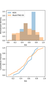 |
Fig. C.3 Same as Fig. 16, but using the morphological sample 2. |
| In the text | |
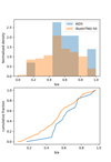 |
Fig. C.4 Same as Fig. 16, but using the morphological sample 3. |
| In the text | |
|
Fig. D.1 Shapes of the groups as a function of number of dwarfs. The panels show the distributions in KiDS (upper panel) and in IllustrisTNG (lower panel) data. |
| In the text | |
Current usage metrics show cumulative count of Article Views (full-text article views including HTML views, PDF and ePub downloads, according to the available data) and Abstracts Views on Vision4Press platform.
Data correspond to usage on the plateform after 2015. The current usage metrics is available 48-96 hours after online publication and is updated daily on week days.
Initial download of the metrics may take a while.