| Issue |
A&A
Volume 705, January 2026
|
|
|---|---|---|
| Article Number | A142 | |
| Number of page(s) | 12 | |
| Section | Planets, planetary systems, and small bodies | |
| DOI | https://doi.org/10.1051/0004-6361/202555173 | |
| Published online | 16 January 2026 | |
True spin-orbit obliquity distribution: Data-driven confirmation of no clustering of misaligned planets
1
Dipartimento di Fisica, Università degli Studi di Milano,
Via Celoria 16,
Milano,
Italy
2
INAF – Osservatorio Astronomico di Brera,
Via E. Bianchi 46,
23807
Merate (LC),
Italy
★ Corresponding author: This email address is being protected from spambots. You need JavaScript enabled to view it.
; This email address is being protected from spambots. You need JavaScript enabled to view it.
Received:
15
April
2025
Accepted:
12
November
2025
Abstract
Context. True spin-orbit obliquities Ψ offer valuable insights into the evolutionary history of exoplanetary systems. Previous studies have suggested that exoplanets tend to occupy either aligned or perpendicular orbits. However, recent research has indicated potential biases caused by the small sample, and has brought into question whether this dichotomy would persist with a larger dataset. Simultaneously, a similar dichotomous behavior has been suggested for Neptune-sized planets.
Aims. Our aim was to investigate the distribution of true spin-orbit obliquities Ψ with an enlarged sample, looking for confirmation of the disputed dichotomy previously found, with a focus also on the obliquities of Neptunes.
Methods. Starting from a sample of 264 projected obliquities λ, we homogeneously computed true obliquities Ψ for 116 planets using the rotation period method. We combined them with four further values gathered from the literature and we then studied their distribution, also as a function of various star-planet system parameters.
Results. Our data-driven work was based on 120 true obliquities Ψ, the largest sample to date, and strongly confirms the presence of a single cluster of aligned planets, followed by an isotropic distribution of misaligned planets with no preferred misalignment. This result is based on a uniform distribution of stellar inclinations i*, for which non-uniformity could have biased previous interpretations of the arrangement of true obliquities. We confirm that Neptunians show a tentative dichotomous distribution with the data available today, but this needs confirmation with an enlarged sample, also because an anisotropic distribution of stellar inclination may be one of the factors hindering the real distribution.
Conclusions. The future increase in the measured Ψ sample over different planet types will allow a better investigation of the relation between misalignment and system properties and will provide a more comprehensive picture of the planetary evolution processes.
Key words: techniques: radial velocities / planets and satellites: dynamical evolution and stability
© The Authors 2026
 Open Access article, published by EDP Sciences, under the terms of the Creative Commons Attribution License (https://creativecommons.org/licenses/by/4.0), which permits unrestricted use, distribution, and reproduction in any medium, provided the original work is properly cited.
This article is published in open access under the Subscribe to Open model. This email address is being protected from spambots. You need JavaScript enabled to view it. to support open access publication.
1 Introduction
The formation and evolution of planetary systems is one of the fundamental questions in modern astrophysics, as it provides key insights into the origin of our Solar System and also the diversity of the thousands of exoplanets discovered in recent decades (Raymond et al. 2020; Kane et al. 2021). It is still an open topic of debate, with many aspects yet to be fully understood (e.g., Mamajek 2009; Mordasini et al. 2012; Turner et al. 2014; Manara et al. 2023). One of the key parameters that can provide valuable insights into planetary formation and evolution is the spin-orbit obliquity, the angle between the stellar rotation axis and the planet orbital plane. It is possible to derive the projected spin-orbit obliquity λ - as projected on the line of sight - via the Rossiter-McLaughlin (RM) effect (Rossiter 1924; McLaughlin 1924), which is an apparent change in the radial velocity curve caused by a planet transiting in front of its host star’s disk (e.g., Triaud 2018). Observational studies of projected spin-orbit obliquities in exoplanetary systems have revealed a diverse range of alignments, suggesting complex dynamical histories. While many hot Jupiters (HJs) exhibit low obliquities, indicating alignment with their host stars’ equatorial planes, a significant fraction display misalignments, including polar and even retrograde orbits (see Albrecht et al. (2022) for a review). Trends have emerged linking obliquity distributions to stellar properties: planets around cool stars (Teff ≤ 6250 K) tend to be well-aligned, whereas those orbiting hotter stars often show a broad range of misalignments, likely due to weaker tidal interactions (Winn et al. 2010; Albrecht et al. 2012; Dawson 2014). Additionally, multi-planet systems and smaller exoplanets generally exhibit lower obliquities (Albrecht et al. 2013; Winn & Fabrycky 2015), suggesting a different dynamical evolution compared to isolated hot Jupiters. Phenomena such as migration (Kley & Nelson 2012) and planet-planet scattering (Rasio & Ford 1996; Weidenschilling & Marzari 1996) are some of the possible explanations for the sometimes dramatically tilted orbits of the exoplanets.
Recent works in the literature have focused on the distribution of true spin-orbit obliquities Ψ, which are obtained by detrending the values of λ from the projection on the line of sight for those systems where it is possible to do this. Some authors have noted a dichotomy in the Ψ distribution, with most planets clustering in aligned orbits (0°-41°) and a non-negligible fraction residing in nearly perpendicular orbits (85°-125°), thus leaving the intermediate spin-orbit inclinations empty (Albrecht et al. 2021). Subsequent works have applied advanced statistical techniques and simulations to investigate how this dichotomy may arise from a biased sample. This bias, possibly caused by the stellar projected rotation velocities v sin i* or the stellar inclination i* selection (Siegel et al. 2023), may obscure the true Ψ distribution. Simulations indicate that the distribution of the projected spin-orbit angle λ serves as a proxy for Ψ, suggesting a true spin-orbit distribution primarily composed of aligned planets, with a sparse population of misaligned ones and no significant clustering at obliquities near perpendicularity (Dong & Foreman-Mackey 2023). However, this has never been verified with actual data, as the sample of planets with measured Ψ was too small. Other authors have also suggested a similar dichotomous trend in the projected obliquity distribution λ of Neptune-sized planets (e.g., Espinoza-Retamal et al. 2024), highlighting how compact systems tend to be aligned (Radzom et al. 2024).
Among the ~6000 confirmed exoplanets as of December 2024, only a few hundred have a λ value, and even fewer have a measure for the true obliquity Ψ (NASA Exoplanet Science Institute 2020). For this work we compiled the most up-to-date catalog of true obliquities by computing them using the rotation period method or by collecting them from the literature. This paper is structured as follows. In Section 2 we detail the rotation period method. In Section 3 we present our comprehensive catalog of exoplanets with λ measures available in the literature. In Section 4 we describe our Markov chain Monte Carlo (MCMC) algorithm, created adopting widely accepted techniques, to compute true obliquity values Ψ via the rotation period method. In Section 5 we analyze the Ψ distribution, and speculate about the correlation with different parameters, such as stellar inclination and stellar age, focusing in particular on Neptune-sized planets. Finally, in Section 6 we discuss the possible mechanisms that could explain the distributions we infer.
2 From projected to true obliquities: The rotation period method
The RM effect provides information about the spin-orbit obliquity angle projected onto the plane of the sky λ, which corresponds to the line-of-sight difference between the host star spin axis and the planet orbital axis (i* and iorb, respectively). The primary challenge to understanding the geometry of planetary systems is to de-project this obliquity from the line of sight in order to obtain the true obliquity Ψ. This can be achieved using the rotation period method, a well-established technique that constrains both the stellar inclination i* and Ψ (e.g., Brown et al. 2012; Masuda & Winn 2020; Albrecht et al. 2021; Bourrier et al. 2023; Bowler et al. 2023; Morgan et al. 2024). We briefly recall here the mathematical framework used to derive Ψ.
We can follow the approach of Fabrycky & Winn (2009) and derive an expression for the cosine of the true obliquity
 (1)
(1)
which depends on the stellar inclination i*, the sky-projected spin-orbit angle λ, and the orbital inclination iorb. Since the RM effect occurs during a planetary transit, one could be tempted to incorrectly assume an orbital inclination iorb ≈ 90°, thus simplifying the previous equation by dropping the last term. In reality, several HJs show inclinations lower than 85°; for example TOI-1431b/MASCARA-5b shows an orbital inclination iorb = $$ (Stangret et al. 2021), whereas HAT-P-56b has  (Zhou et al. 2016). Considering that a drop of ~10° around 90° produces a variation of 17% in the value of the cosine, properly accounting for them is crucial for a correct inference.
Neglecting the star’s differential rotation, we can define the equatorial velocity of the host star as
 (2)
(2)
and with this we can express sin i* as
 (3)
(3)
where Prot is the stellar rotation period, v sin i* is the stellar rotational velocity projected along the line of sight, and R* is the stellar radius. A nice visualization of this geometry is given in Fig. 1 of Albrecht et al. (2022).
Theoretically, the stellar inclination i* could also be constrained using different approaches. Late-type stars can have their i* determined through asteroseismology (Gizon & Solanki 2003; Ballot et al. 2006) in a complementary fashion with respect to the RM, thus also providing higher precision. However, this technique is possible only for bright stars; its reliability is strongly affected by biases when the signal-to-noise ratio of the power spectra is low (Kamiaka et al. 2018). Another method of determining λ and i* is to analyze the possible asymmetry of transit light curves, which is caused by gravity darkening (Barnes 2009).
For the sake of homogeneity, we opted to use Equation (1) for the creation of our sample where possible. When the stellar rotation period - or other quantities derived in Equation (1) - is not available, we used the literature values of Ψ estimated through other methods.
3 Creating a catalog: Sample selection
We started the creation of our sample of obliquities with the 235 planets with available λ values in the TEPCat catalog1 (Southworth 2011) as of December 2024. We then extended the sample by adding 21 additional planets from the NASA Exoplanet Archive2 (NASA Exoplanet Science Institute 2020; Christiansen et al. 2025), hereafter referred to as NEA. When multiple λ values were available for the same planet, we considered the most recent, precise, and comprehensive sources as more eligible.
A bibliographic search allowed us to retrieve 18 more λ values that were still not present in the catalogs, most likely because they were recently published. These values were obtained for the planets TOI-2145b (Dong et al. 2024); TOI-2119b (Doyle et al. 2024); TOI-1694b (Handley et al. 2025); TOIs 558b, 2179b, 4515b, and 5027b (Espinoza-Retamal et al. 2025); TOI-1259Ab (Veldhuis et al. 2025); TOI-1759Ab (Polanski et al. 2025); TOI-2364b (Tamburo et al. 2025); TOI-3714b and TOI-5293Ab (Weisserman et al. 2025); K2-237b (Zak et al. 2025a); and HAT-P-50b, Qatar-4b, TOI-2046b, WASP-48b, and WASP-140b (Zak et al. 2025b). This resulted in a total of 274 individual planets (orbiting 265 stars) with known projected obliquity λ. For systems hosting multiple planets, we restricted our analysis to a single planet as mutual inclinations are beyond the scope of this study. We ended up with 264 planets with known projected obliquity λ, 71 of which also have a published true obliquity Ψ. The only missing λ is Kepler-408b as we were only able to retrieve its Ψ value from Kamiaka et al. (2019).
We aimed at uniformly computing Ψ from the literature values of λ for all the planets of our sample. To this end, we needed reliable, and possibly homogeneous, estimates of stellar radii (R*), stellar rotational periods (Prot), and stellar projected rotational velocities (v sin i*) to derive stellar inclinations i* (see Equation (3)), and subsequently Ψ, as shown in Equation (1).
3.1 Stellar rotation periods
The stellar rotation period was the most limiting parameter in our work. After an extensive bibliographic search, we were able to recover the rotation periods Prot only for 120 host stars. This is due to the need to observe long photometric time series (up to several months of observations) to obtain Prot. The stellar rotation period is derived from the modulation of the stellar brightness due to the presence of magnetically active regions on the stellar rotating surface: non-active stars (e.g., hot A-F type stars) may lack any feature that allows us to derive the stellar rotation, while very active stars (e.g., young stars or M-type stars) may present a large number of spots and/or faculae that may lead to misidentifying Prot. Additionally, a partial or inhomogeneous observing window may cause an alias of the Prot being identified as the true rotational period (Basri & Shah 2020). The presence of differential rotation may also lead to incorrect Prot values (Aigrain et al. 2015).
Regarding the literature values of our sample, one host star exhibited multiple Prot measurements. Three more had rotation periods either reported without uncertainties or only as an upper limit. In detail, we found the following:
WASP-60 (Mancini et al. 2018): two compatible Prot values were provided (Prot,1 = 31.8 ± 1.9 days and Prot,2 = 34.8 ± 2.7 days); we conservatively assigned the semi-difference of the maximum range as the uncertainty for the central value (Prot = 33.3 ± 3.8days).
HD 17156 (Fischer et al. 2007): the rotation period was provided without uncertainties (Prot = 12.8 days), so we supplemented it with a conservative 10% uncertainty, a typical uncertainty for F- and G-type stars (Santos et al. 2021).
WASP-180a (Temple et al. 2019): the literature provided only an upper limit on the rotation period (Prot < 3.3 days), due to the presence of its co-moving companion, WASP-180B, which complicates measurements. We allowed the value to span from the upper limit down to the break-up period of 0.1 days.
KELT-18 (Rubenzahl et al. 2024): similarly to the previous case, the literature provided only an upper limit. We allowed the value to span from this upper limit to the break-up period of 0.4 days.
3.2 Stellar radii
Stellar radii may be computed with very different methods. The most precise measurements are those obtained using interferometry and asteroseismology, or for eclipsing binary stars (Moya et al. 2018). The latter are absent from our sample, while interferometry and asteroseismology may be used only on a limited sample of bright targets. Stellar radii may also be derived from photometric data; in this case, a good estimate of the distance and the interstellar extinction is crucial. Photometric radii are the most commonly found in the literature, but the data may be obtained via many different instruments.
In this work, we decided to use the radii given in the Gaia DR3 Astrophysical Parameters Archive3, to ensure the most homogeneous and precise set possible. Two values of R* are present in the archive, the GSP-Phot and the FLAME R*. The first are computed using the state-of-the-art Gaia parallaxes, and the photometric and spectroscopic Gaia data (the low-resolution BP/RP spectra and the apparent G magnitude), while the latter are a refinement built on the photometric and the spectroscopic Gaia data (van Leeuwen et al. 2022). We used the GSP-Phot values for our sample. We note, however, that the two sets of values are in very good agreement.
Our sample consists of 265 planets. In 22 cases, we were unable to retrieve Gaia information, and thus we had to use literature values. However, the final sample will have only 12 true obliquities computed without Gaia radii (10%), because of the lack of parameters needed to compute Equation (1), hence granting a high degree of homogeneity. In the end, between Gaia DR3 and the literature search, we were able to estimate the stellar radii for all the 265 stars in our sample.
3.3 Projected rotational velocities and orbital inclinations
Projected rotational velocities (v sin i*) were taken from the same analyses providing the sky-projected obliquity λ, whenever available. These values often combine spectroscopic v sin i* measurements with the additional constraints from the Rossiter-McLaughlin effect, which can lead to improved precision, especially at low v sin i*, compared to estimates derived from CCFs alone. We were able to retrieve 264 projected rotational velocities v sin i*.
Similarly to v sin i*, we preferably gathered orbital inclinations from the same paper originating information about λ, to ensure homogeneity, for a total of 263 iorb.
In the end, our sample of 265 planets, 71 of which had a Ψ measure available, presented 264 projected obliquities λ, 265 stellar radii R* (243 of which from Gaia DR3 Astrophysical Parameters), 264 v sin i*, and 120 rotation periods Prot. We were able to obtain the complete set of all four values for 119 planets. Kepler-408 b is missing both λ and v sin i*, but we have information about its star’s rotation period.
3.4 True obliquities Ψ from the literature
Our literature search turned out eight more Ψ values for planets where we were not able to recover all the information needed for the rotation period method, bringing our total sample of planets with information on Ψ - or on the parameters used to infer it -to 127 Ψ.
Siegel et al. (2023) proved that gravity darkening (GD) is biased toward perpendicular orbits, so we decided to exclude seven measurements from our sample, because their obliquity, either projected or true, was extracted via GD. For four of these seven measurements we only had information about the true obliquity (all four parameters needed to apply the rotation period method were missing): HATS-70 b (Zhou et al. 2019), KELT-17 b (Zhou et al. 2016), KELT-19 b (Kawai et al. 2024), Kepler-1115 b (Barnes et al. 2015). For the remaining three measurements, the literature provided all the parameters required for our analysis: KOI-13 b (Howarth & Morello 2017), Kepler-462 b (Ahlers et al. 2015), and MASCARA-1 b (Hooton et al. 2022).
It is worth noting that, within the limited sample of planetary obliquities measured via GD, some systems also have obliquity determinations from the RM effect, which yield results in close agreement (e.g., KELT-9 b (Borsa et al. 2019; Ahlers et al. 2020; Stephan et al. 2022) or MASCARA-4 b (Ahlers et al. 2020; Zhang et al. 2022).
With these final modifications we had no GD measurements in our sample, and a total of 116 planets for which the rotation period method is applicable, supplemented by four more true obliquities Ψ found in the literature: HD 89345 b (Bourrier et al. 2023), KELT-9 b (Stephan et al. 2022), Kepler-408 b (Kamiaka et al. 2019), and WASP-131 b (Doyle et al. 2023). The first true obliquity was detected via RM combined with a PDF for i* from Van Eylen et al. (2018); the second was detected via Doppler tomography (DT); the third had its stellar inclination determined via asteroseismology (e.g., Ulrich 1986; Aerts et al. 2010), and the fourth via the reloaded Rossiter-McLaughlin (RRM Cegla et al. 2016) technique.
An extract of our dataset is available in Table A.1 and in machine-readable form at CDS in its complete form. It also includes the results of our analysis, detailed in the following section.
4 Inferring true obliquities
We computed the true obliquities using a robust MCMC algorithm. First, we computed the stellar inclinations exploiting Equation (3), accounting for the inherent correlation between veq and v sin i* highlighted by Masuda & Winn (2020), necessary for every inference involving these two values (e.g., i* and Ψ as in this work). The approach we adopted also follows the methodology detailed in Appendix A of Bowler et al. (2023). It was performed assuming uniform priors on v sin i*, R*, Prot, along with an isotropic (sin i*) prior on the stellar inclination. We tested our MCMC algorithm to extract stellar inclinations i* on the Morgan et al. (2024) dataset, yielding great compatibility among the i* results (p-value = 1.0), as shown in Fig. 1. Finally, by incorporating a uniform prior on the projected obliquity λ, we extracted true obliquities Ψ4 using Equation (1).
The task of extracting true obliquities from projected obliquities has been undertaken by several authors, including Albrecht et al. (2021). We tested our algorithm on their dataset of planets with computable (R*, Prot, v sin i* and λ) true obliquities Ψ, and obtained excellent agreement between the two results, as illustrated in Fig. 2. In 63 cases our computed true obliquities had a counterpart in studies other than Albrecht et al. (2021), four of which were only upper limits, namely HAT-P-36 b (Mancini et al. 2015), Kepler-17 b (Désert et al. 2011), WASP-43 b (Esposito et al. 2017), and TOI-113 6 d (Dai et al. 2023). We also compared the results of the MCMC algorithm with 59 of these values, and found good agreement: a Pearson test yielded a 0.99 correlation rank with a p-value order of magnitudes lower than the threshold of 0.05 to reject the null hypothesis of data being uncorrelated. As the radii values were mostly taken not from the work from which we gathered λ and v sin i* (Fig. 3), and since the literature Ψ values do not represent a homogeneously derived sample, we obtained p-values lower than the above-mentioned threshold while performing an ordinary linear regression. Hence, we can conclude that our inference method is consistent with other works when we apply it on their dataset (Albrecht et al. 2021; Morgan et al. 2024), and it yields coherent results with the literature values. The four excluded upper limits are compatible with our results. Therefore, we decided to adopt the literature values for the true obliquity only if one of the parameters mentioned in Section 3 was missing, thus preventing us from calculating that obliquity.
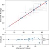 |
Fig. 1 Comparison between our stellar inclinations i* and those computed by Morgan et al. (2024), starting from the same dataset. The gray dashed lines represent the y = x relation, whereas the solid red line represents the linear fit, and the shaded red region represents the 68% confidence interval. The residuals are computed with respect to the fit relation. Uncertainties in the residuals panel are omitted to ensure better readability. |
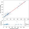 |
Fig. 2 Comparison between our true obliquities and those computed by Albrecht et al. (2021). Starting from the same dataset, we achieve an excellent agreement within the 68% confidence interval of the linear fit. The gray dashed line represents the y = x relation. The linear correlation is guaranteed by a χ2 test yielding p = 1.0, allowing the rejection of the null hypothesis that the data are not linearly correlated. The residuals are computed with respect to the fit line. Uncertainties in the residuals panel are omitted to ensure better readability. The presence of outliers is due to our inability to recover the iorb values used by Albrecht et al. (2021), but also highlights their importance for a correct inference. |
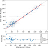 |
Fig. 3 Comparison between the true obliquities computed in this work and the corresponding literature values, where available, but excluding Albrecht et al. (2021). The figure adopts the same plotting style as Fig. 2. The plot is made assuming the conventional stellar inclination (i* ≤ 90°). |
5 Results
In Fig. 4 we show the distribution of our 120 Ψ values, which doubles the observational sample of 57 planets presented in Albrecht et al. (2021). Only a cluster of aligned planets is present, with no significant density around perpendicular orbits. Our results thus confirm with observational data what was previously supposed by Siegel et al. (2023) and Dong & Foreman-Mackey (2023).
We examined the robustness of our analysis, particularly concerning the disputed lack of planets in the 90°-100° range, both in the posterior probability histogram and in the distribution of central values (Fig. 4, top and middle panels). After testing different kernels and bandwidth selections (Scott 1992; Silverman 2018) - which had no significant impact on the overall shape -we adopted an averaged histogram with variable binning (bottom panel). Specifically, we computed 100 histograms with 20 bins, introducing 20% bin variability to mitigate both overfitting and oversmoothing. This approach reduced the apparent valley in the perpendicularity range. Finally, we computed a kernel density estimation (KDE) on the now smoother average histogram, which presented a single prominent peak for aligned orbits.
We performed a Kolmogorov-Smirnov (K-S) test with the null hypothesis that the Ψ distribution from Albrecht et al. (2021) is the same as the distribution of our dataset, using a significance level of p = 0.05. The resulting p-value did not allow us to reject the null hypothesis. This does not change our conclusions because small sample sizes can lead the K-S test to not reject the null hypothesis even though two distributions differ. An alternative could be an Anderson-Darling test (A-D test Anderson & Darling 1952, 1954), which places more weight on the tails of the distribution without relying only on the maximum spacing among them (Darling 1957; Scholz & Stephens 1987; Makarov & Simonova 2017). The A-D test rejected the null hypothesis of the two samples being drawn from the same distribution with a p-value of p = 8 ∙ 10−4. However, we note that this result could be biased by an overall small sample, of barely more than a hundred planets. Hence, considering that Albrecht et al. (2021) had suggested that true obliquities cluster on aligned and perpendicular orbits, we performed a dip-test for uni-modality (Hartigan & Hartigan 1985) on their sample. As expected, we can reject the null hypothesis of their sample being drawn from a uni-modal distribution at the 1% level, whereas our sample has a p-value of 0.91. These facts highlight how our Ψ sample differs from that of Albrecht et al. (2021) in terms of modality of the distribution (Fig. 5), being close to what is expected in the more recent literature (Dong & Foreman-Mackey 2023). It should be noted, and it is reasonable to expect, that with a larger sample size the K-S test would also reject the null hypothesis.
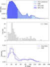 |
Fig. 4 Distribution of the 120 true obliquities present in our sample. In the top panel, the Ψ values are shown as a superposition of their normalized posteriors, fitted with a kernel density estimation (KDE) with a Gaussian kernel and Silverman’s bandwidth (other bandwidth selections yielded similar results or overfitted graphs). The shaded blue and light blue regions respectively represent the 68 and 95% highest density intervals (HDIs). The middle panel displays a simple histogram of true obliquities. The lower panel addresses two key issues: (i) the arbitrariness of binning; (ii) the apparent valley around 90°–100°. To account for these issues, 100 histograms with 20 bins were generated, with 20% variability on their boundaries. The average histogram is represented by the solid blue line, while the dashed blue line represents the KDE. |
5.1 Stellar inclination distribution
Our algorithm also provided information about the stellar inclination distribution within our sample, shown in Fig. 6. This was possible only for the 116 systems for which we computed Equation (1), along with HD 89345 b and WASP-131 b for which we were able to retrieve information about i*, for a total of 118 planets. We investigated i* as the possible bias that led Albrecht et al. (2021) to identify the dichotomy shown in the right marginal histogram of Fig. 7, as suggested by Dong & Foreman-Mackey (2023) and Siegel et al. (2023). By recomputing stellar inclinations and true spin-orbit obliquities for the 51 planets with R*, Prot, v sin i*, and λ available in their dataset, we identified two key factors: (i) the sample size and (ii) the diversity of stellar inclinations. Our sample is significantly larger (+127%) and our stellar obliquities are more evenly distributed across the admissible range 0°-90°. We confirmed this trend in Fig. 8.
By removing stellar inclinations lower than 35°, a reasonable threshold when comparing the i* distributions between Figs. 6 and 7, we were able to reproduce an apparent dichotomy while minimizing data loss (only 12 planets were removed).
Considering that leading theories of planetary formation predict that planets form in approximately aligned orbits within an approximately aligned protoplanetary disk (e.g., Ida & Lin 2004; Armitage 2010), it is reasonable to expect that most planets will remain on aligned orbits. This expectation holds particularly for perpendicular stellar inclinations. Conversely, the detection of an exoplanet - and a subsequent RM measure - can only occur if the planet transits in front of its host disk. Thus, stellar inclinations closer to a pole-on configuration (i* ~ 0°) imply that the planet will be on a misaligned orbit (Campante et al. 2016). This, combined with a large sample size, can manifest a noticeable peak on aligned orbits with a more uniform spread at other angles.
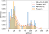 |
Fig. 5 Comparison between the dataset of Ψ from Albrecht et al. (2021) and that of this work. An A-D test provided evidence that the two distributions significantly differ, along with a dip-test for uni-modality proving that the Albrecht et al. (2021) distribution of true obliquities is consistent with a multi-modal distribution, while our sample of true obliquities is consistent with a uni-modal distribution. KDEs are plotted for ease of visualization. |
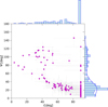 |
Fig. 6 True spin-orbit obliquities of our sample of 118 planets with respect to the stellar inclination. The marginal histograms show a peak for perpendicular stellar inclinations i* (top) and a peak for aligned orbits followed by a near-uniform distribution for misaligned orbits (right). The marginal histogram for Ψ is binned every 5° and is fitted with a KDE with a Gaussian kernel and Silverman’s bandwidth. |
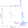 |
Fig. 7 True spin-orbit obliquities from Albrecht et al. (2021) with respect to stellar inclination. We were able to recompute a total of 51 Ψ values, thanks to the availability of the quantities in Equation (1). The marginal histogram on the right (binned every 5° and fitted with a KDE using a Gaussian kernel and Silverman’s bandwidth) highlights a dichotomy in true obliquities, while the top marginal histogram emphasizes the non-uniformity of stellar inclinations i*. |
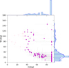 |
Fig. 8 Recreation of the apparent dichotomy found by Albrecht et al. (2021) with respect to stellar inclination. In this figure, as in the previous figure, we approximately recreated an apparent dichotomy for true obliquities Ψ by removing only 12 planets from the 118 available. This result underscores the importance of uniformity of stellar inclinations i*. Low stellar inclinations i* are key to obtaining uniformity on misaligned values of Ψ. |
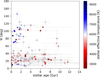 |
Fig. 9 Distribution of obliquities Ψ with respect to stellar age for our sample. 119 planets are plotted; K2-105 was excluded because its age estimate is not available in the literature. |
5.2 True obliquities vs. stellar age
Since true obliquity can serve as a proxy for the dynamical evolution of an exoplanetary system, we investigated whether it correlates with stellar age. Stellar age is a notoriously challenging parameter to measure with high precision (Soderblom 2010). After an extensive literature search, we identified the stellar age for all of the 120 stars for which we had a true obliquity Ψ available, except one (K2-105), for a total of 119 stars.
In Fig. 9 we analyze the relation between Ψ, the stellar age, and the stellar effective temperature. Defining misaligned planets as those with an obliquity greater than 41°, the angle beyond which there can be von Zeipel-Kozai-Lidov cycles (ZKL, von Zeipel 1910; Kozai 1962; Lidov 1962), we find a predominance of misaligned planets among stars younger than 5 Gyr, with minor exceptions. The existence of two subpopulations in Fig. 9 is evident: one consisting of young and aligned planets, and the other of young and misaligned planets. Older misaligned planets do not contribute significantly, primarily due to the large uncertainties associated with their age estimates. Additionally, aligned planets systematically exhibit lower host star temperatures compared to misaligned ones. This latter interpretation, however, is likely biased by the stellar age itself, as higher temperatures are not expected for old stars.
We are not able to extract any conclusion regarding the relation between obliquity and stellar age, except for the already known fact that planets tend to damp obliquity over time via several mechanisms (or a combination of mechanisms), such as tidal dissipation (Ogilvie 2014; Lin & Ogilvie 2017), von Zeipel-Kozai-Lidov cycles in the presence of a distant perturber (von Zeipel 1910; Kozai 1962; Lidov 1962; Katz et al. 2011), and secular interactions (Saillenfest et al. 2019). However, we found a cluster of older and misaligned planets that warranted investigation.
Planets with uncertain mass measurements, divided by planet type.
5.3 A focus on Neptunian planets
The small number of rocky planets in our sample did not allow us to proceed with further analysis on them. Following Stevens & Gaudi (2013) classification, we focused on Neptunes (10-100 M⊕), Jupiters (100-1000 M⊕), and super Jupiters (1000-4131 M⊕). For a few planets, robust mass estimates were not available. In these cases we consulted the literature to make an informed choice, as summarized in Table 1 (e.g., K2-33 b, where the reported limits and simulations suggest a Neptunian nature). The result is shown in Fig. 10. Several authors have reported correlations between projected obliquities of hot Jupiters and stellar effective temperature (e.g., Winn et al. 2010; Albrecht et al. 2012, 2022). Specifically, they observed a sudden increase in λ beyond the Kraft break at Teff ≈ 6250 K (Kraft 1967), a threshold beyond which the convective envelope becomes nearly negligible (Pinsonneault et al. 2001). With minor exceptions, our findings confirm the same trend in our sample for gaseous giants (Fig. 10, middle and right panels).
For Neptunes we noted a conspicuous number of planets on misaligned orbits, specifically 11 out of 32. This finding is in good agreement with previous works regarding the stability of misaligned orbits - especially polar - for Neptunes (Louden & Millholland 2024). We found that most of the old and misaligned planets in our dataset are part of the Neptunian subsample. This pattern led us to further investigate the underlying mechanisms that could produce such orbital configurations.
Some authors (Batygin 2012; Lai 2014) found that misalignment may be caused by an interaction with a binary companion. Conversely, other authors suggested that multi-star exoplanetary systems could favor aligned orbits (Christian et al. 2022; Rice et al. 2024). Specifically, the interaction between two moderately distant protoplanetary disks may lead to alignment. We first examined the literature for evidence of stellar companions to the hosts of our misaligned Neptunes. Our small sample of misaligned Neptunes consisted of 11 planets. In our sample, two misaligned planets showed evidence of a binary companion: WASP-131 b, whose companion has been detected with different observations (Bohn et al. 2020; Southworth et al. 2020; Zak et al. 2024), and K2-290, a star in a triple system orbited by two coplanar and retrograde planets (Hjorth et al. 2019, 2021; Best & Petrovich 2022). Two more aligned planets have a binary companion, namely DS Tuc A b (Zhou et al. 2020) and Kepler-25 c (Bourrier et al. 2023).
Some authors (Espinoza-Retamal et al. 2024) starting from a sample of 27 Neptune projected obliquities λ applied a HBM framework from Dong & Foreman-Mackey (2023) and found tentative evidence of a dichotomous behavior in the posterior Ψ distribution, although the result was defined as prior dependent. The same dichotomy was found using a subsample of 17 Neptunes with available Ψ on TEPCat.
We analyzed our sample of Neptunian planets perturbing their Ψ values in their uncertainty bounds 1000 times, using split-normal distributions. We fitted each synthetic sample with a two-component Gaussian distribution and we extracted the median values for the parameters of the Gaussian distributions φi = N(μi ,σi) and their relative weights w, as well as the 16th and 84th percentiles. The result, shown in Fig. 11, suggests the presence of two main components,  and
and  , of relative weights w1 = 0.66 ± 0.06 and w2 = 0.34 ± 0.06, further supported by an Ashman value of
  , well beyond the D > 2 rule of thumb indicating that the two components are clearly separated (Ashman et al. 1994). However, a dip-test conducted on this sample was unable to reject the unimodality of the distribution. Thus, these tests mildly corroborate the existence of a dichotomy in the largest Neptunian Ψ sample currently available, although the sample size is still too small to draw anything but tentative conclusions. Moreover the stellar inclination distribution of Neptunian planets shows clear signs of anisotropy (Fig. 12), while both the results and marginal distributions of the whole sample without the Neptunes remain unchanged. A larger sample of Neptunes is surely needed to extract definitive conclusions regarding their distributions in the Ψ space.
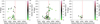 |
Fig. 10 Relation between true obliquity Ψ and stellar effective temperature Teff for different planet subgroups. The red dashed line shows the Kraft break temperature at T = 6250 K, first highlighted by Winn et al. (2010). In the left panel Neptunes divide almost equally between aligned and misaligned, with older planets populating even the high-obliquity region. The middle and right panels show the behavior of Jupiters and superJupiters. The misaligned planets are younger, and they are almost never found well before the Kraft break. |
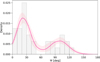 |
Fig. 11 True obliquity distribution of the subsample of 28 Neptunes. The pink solid line represents the best fitting two-component Gaussian mixture model, obtained after 1000 perturbations of the planetary obliquities in their uncertainty range. The shaded light pink area represents the 68% CI. The two components are well separated by an Ashman factor D = 4.33. |
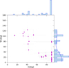 |
Fig. 12 True spin-orbit obliquities for our sample of 32 Neptunes with respect to the stellar inclination. In this figure, following the same fashion of previous plots, we note (i) how the dichotomous behavior of true obliquities is accompanied by a non-uniform distribution of stellar obliquities and (ii) how the statistics are still too low to draw robust conclusions. |
6 Discussion and conclusions
Starting from a sample of 264 projected spin-orbit obliquities λ collected from TEPCat, the NASA Exoplanet Archive, and additional literature sources, we were able to homogeneously compute 116 true obliquities Ψ through the rotation period method. Together with four additional values taken directly from the literature, and after excluding those derived via GD, due to its known bias toward perpendicular orbits (Siegel et al. 2023), this results in a final de-biased sample of 120 planets. This dataset doubles the size of the previous compilation by Albrecht et al. (2021) and constitutes the largest collection of true spin-orbit obliquities available to date. The main results emerging from the analysis of this enlarged sample are outlined in the following subsections.
6.1 No clustering of misaligned orbits
Our primary goal was to shed light on the true spin-orbit obliquity distribution of exoplanets using a data-driven approach. This was achieved by correctly inferring stellar inclinations i* (Masuda & Winn 2020; Bowler et al. 2023; Morgan et al. 2024), which allowed us to extract the true obliquities following Equation (1) (e.g., Fabrycky & Winn 2009; Albrecht et al. 2021; Knudstrup et al. 2024). Albrecht et al. (2021) noted a dichotomy in the distribution of Ψ, with two distinct clusters roughly within the ranges Ψ = 0°-41° and Ψ = 80°-125°. This conclusion, which relies on a still uncertain theoretical foundation (Albrecht et al. 2021), has been questioned by some teams (Siegel et al. 2023; Dong & Foreman-Mackey 2023), whose subsequent work has attempted, so far unsuccessfully, to resolve it (Knudstrup et al. 2024). However, Siegel et al. (2023) and Knudstrup et al. (2024) pointed out that stellar inclination i* could significantly bias the studied sample.
In this work we provide strong evidence against the existence of two peaks for aligned and perpendicular orbits, finally supporting with observational data the idea of a single peak for equatorial planets followed by an isotropic distribution on misaligned obliquities (Siegel et al. 2023; Dong & Foreman-Mackey 2023). This is granted by a dip-test rejecting the null hypothesis of uni-modality at the 1% level. Although this conclusion was reached without relying on GD measurements, future works - based on a significantly larger number of GD determinations when available - could provide interesting insights into the impact of this technique on the overall exoplanet sample from a data-driven perspective.
6.2 Stellar inclination bias
In particular, in this work we showed how i* can heavily bias the Ψ distribution: RM measurements are performed during transits, so configurations with i* ~ 0° are more likely to host misaligned planets, whereas configurations with i* ~ 90° favor aligned orbits. Unlike Albrecht et al. (2021), our sample is characterized by more uniform stellar inclinations. Even a small non-uniformity, such as removing inclinations lower than 35°, can recreate the apparent dichotomy observed in the aforementioned work. This corroborates from a data-driven perspective a bias that was theorized in previous research (Siegel et al. 2023; Dong & Foreman-Mackey 2023).
6.3 A tentative Neptunian dichotomy
Our 120-planet sample presents a sub-sample of 32 planets belonging to the Neptunian realm, according to the Stevens & Gaudi (2013) classification (10 < Mnep∕M⊕ < 100). Among these, 11 show signs of misalignment, defined as being more than 1σ from 41°, the limit beyond which ZKL cycles can shape the planetary system architecture in the case of a massive companion. In this regard, our analysis found evidence of a stellar companion only for four Neptunians, detailed in Section 5.3, among which two show signs of misalignment. Previous authors (Petrovich et al. 2020; Espinoza-Retamal et al. 2024) have found tentative evidence of a dichotomous behavior of the true obliquity distribution of Neptunes, basing their work on projected obliquities λ. With a larger sample of true obliquities we can robustly state that a multi-Gaussian fit yields two distributions peaked at ~20° and ~100° and clearly separated by an Ashman D value of 4.33 after a two-Gaussian fit. However, a Hartigan’s dip-test (Hartigan & Hartigan 1985) was not able to reject the hypothesis of uni-modality for this distribution, likely because of the still small sample.
We could not help but notice that this dichotomy very much resembles what Albrecht et al. (2021) found for the whole sample of exoplanets. A Neptunian sample half the size of the one used by Albrecht et al. (2021), combined with a failed dip-test might suggest that a larger sample is needed to draw definitive conclusions, as low statistics can hinder the reliability of p-values by masking effects that a larger sample will show. This conclusion agrees with the results of Espinoza-Retamal et al. (2024), which detailed how the posterior distribution of Neptunian true obliquities is sensitive to hyperpriors in the Dong & Foreman-Mackey (2023) hierarchical Bayesian framework, whereas Jupiters tend to cluster on aligned orbits with an isotropic tail on larger obliquities without strongly responding, and modifying the overall trend, to hyperpriors.
Albrecht et al. (2021) noted how theoretical foundations failed to justify their reported dichotomy; however, they highlighted how secular resonance crossing in the presence of a massive outer companion could provide theoretical support for the presence specifically of perpendicular Neptunes, similarly to ZKL cycles (Petrovich et al. 2020). In our sample only one planet presents an outer companion while being misaligned, and hence we can suggest this as a possible mechanism for misalignment. Several mechanisms beyond ZKL have been proposed to explain misalignment, such as primordial misalignment (Bate et al. 2010) and magnetic torques (Lai et al. 2011) (see Albrecht et al. (2022) for a review). Other works have highlighted that when specific conditions occur, Neptunians can show peculiar architectures: compact Neptunian systems tend to be more aligned (Radzom et al. 2024; Polanski et al. 2025); Neptunians are less responsive to tides, and hence their longer realignment timescales can doom the planet to reside in a misaligned orbit (Handley et al. 2025); and polar Neptunes can be so unresponsive to tides that they retain their perpendicular obliquity (Louden & Millholland 2024).
The measurement of spin-orbit angles for Neptune-sized planets is particularly valuable as their obliquities may provide crucial clues to the dynamical histories of intermediate-mass planets, a still underrepresented population that appears to show intriguing differences from hot Jupiters. The ongoing interest for Neptunes, along with future missions to characterize small planets (PLATO Rauer et al. 2025) and exoplanetary atmospheres (ARIEL Tinetti et al. 2018), will dramatically increase our knowledge of the formation and evolution of exoplanets with the fresh data they are expected to produce in the next years.
Data availability
An extract of the data used in this work is shown in Table A.1. The full table is available at the CDS via https://cdsarc.cds.unistra.fr/viz-bin/cat/J/A+A/705/A142.
Acknowledgements
We deeply thank the referee for their constructive and insightful comments, which greatly contributed in improving the quality of this work. AMR gratefully thanks M. Frangiamore for the enlightening conversations during these months. F.B. acknowledges support from Bando Ricerca Fondamentale INAF 2023 and from PLATO ASI-INAF agreement n. 2022-28-HH.0. S.F. acknowledges financial contribution from the European Union (ERC, UNVEIL, 101076613), and from PRIN-MUR 2022YP5ACE. Views and opinions expressed, however, are those of the author(s) only and do not necessarily reflect those of the European Union or the ERC. Neither the European Union nor the granting authority can be held responsible for them. This work has made an extensive use of TEPCat by John Southworth, Keele University, UK. This research has made use of the SIMBAD database, operated at CDS, Strasbourg, France (Wenger et al. 2000). This research has made use of the NASA Exoplanet Archive, which is operated by the California Institute of Technology, under contract with the National Aeronautics and Space Administration under the Exoplanet Exploration Program (NASA Exoplanet Science Institute 2020). This research has made use of data obtained from or tools provided by the portal exoplanet.eu of The Extrasolar Planets Encyclopedia. This work has made use of data from the European Space Agency (ESA) mission Gaia (https://www.cosmos.esa.int/gaia), processed by the Gaia Data Processing and Analysis Consortium (DPAC, https://www.cosmos.esa.int/web/gaia/dpac/consortium). Funding for the DPAC has been provided by national institutions, in particular the institutions participating in the Gaia Multilateral Agreement (European Space Agency (ESA) & DPAC Consortium 2022). This research has made use of the Astrophysics Data System, funded by NASA under Cooperative Agreement 80NSSC21M00561. Software. The code associated with this work used only open source software. This research made use of ASTROQUERY (Ginsburg et al. 2019), EMCEE (Foreman-Mackey et al. 2013), CORNER.PY (Foreman-Mackey 2016), MATPLOTLIB (Hunter 2007), NumPy (Harris et al. 2020), PANDAS (pandas development team 2024), SciPy (Virtanen et al. 2020), SCHWIMMBAD (Price-Whelan & Foreman-Mackey 2017), SEABORN (Waskom 2021).
References
- Aerts, C., Christensen-Dalsgaard, J., & Kurtz, D. W. 2010, Asteroseismology (Berlin: Springer) [Google Scholar]
- Ahlers, J. P., Barnes, J. W., & Barnes, R. 2015, ApJ, 814, 67 [CrossRef] [Google Scholar]
- Ahlers, J. P., Johnson, M. C., Stassun, K. G., et al. 2020, AJ, 160, 4 [NASA ADS] [CrossRef] [Google Scholar]
- Aigrain, S., Llama, J., Ceillier, T., et al. 2015, MNRAS, 450, 3211 [Google Scholar]
- Albrecht, S., Winn, J. N., Johnson, J. A., et al. 2012, ApJ, 757, 18 [NASA ADS] [CrossRef] [Google Scholar]
- Albrecht, S., Winn, J. N., Marcy, G. W., et al. 2013, ApJ, 771, 11 [NASA ADS] [CrossRef] [Google Scholar]
- Albrecht, S. H., Marcussen, M. L., Winn, J. N., Dawson, R. I., & Knudstrup, E. 2021, ApJ, 916, L1 [NASA ADS] [CrossRef] [Google Scholar]
- Albrecht, S. H., Dawson, R. I., & Winn, J. N. 2022, PASP, 134, 082001 [NASA ADS] [CrossRef] [Google Scholar]
- Alonso, R., Auvergne, M., Baglin, A., et al. 2008, A&A, 482, L21 [NASA ADS] [CrossRef] [EDP Sciences] [Google Scholar]
- Anderson, T. W., & Darling, D. A. 1952, Annal. Math. Stat., 23, 193 [Google Scholar]
- Anderson, T. W., & Darling, D. 1954, J. Am. Stat. Assoc., 49, 765 [Google Scholar]
- Armitage, P. J. 2010, Astrophysics of Planet Formation (Cambridge: Cambridge University Press) [Google Scholar]
- Ashman, K. M., Bird, C. M., & Zepf, S. E. 1994, AJ, 108, 2348 [Google Scholar]
- Ballot, J., García, R. A., & Lambert, P. 2006, MNRAS, 369, 1281 [Google Scholar]
- Barnes, J. W. 2009, ApJ, 705, 683 [Google Scholar]
- Barnes, J. W., Ahlers, J. P., Seubert, S. A., & Relles, H. M. 2015, ApJ, 808, L38 [NASA ADS] [CrossRef] [Google Scholar]
- Basri, G., & Shah, R. 2020, AJ, 901, 14 [Google Scholar]
- Bate, M. R., Lodato, G., & Pringle, J. E. 2010, MNRAS, 401, 1505 [NASA ADS] [CrossRef] [Google Scholar]
- Batygin, K. 2012, Nature, 491, 418 [NASA ADS] [CrossRef] [Google Scholar]
- Benatti, S., Damasso, M., Borsa, F., et al. 2021, A&A, 650, A66 [NASA ADS] [CrossRef] [EDP Sciences] [Google Scholar]
- Best, S., & Petrovich, C. 2022, ApJ, 925, L5 [NASA ADS] [CrossRef] [Google Scholar]
- Bieryla, A., Zhou, G., García-Mejía, J., et al. 2024, MNRAS, 527, 10955 [Google Scholar]
- Bohn, A. J., Southworth, J., Ginski, C., et al. 2020, A&A, 635, A73 [NASA ADS] [CrossRef] [EDP Sciences] [Google Scholar]
- Bonomo, A. S., Desidera, S., Benatti, S., et al. 2017, A&A, 602, A107 [NASA ADS] [CrossRef] [EDP Sciences] [Google Scholar]
- Borsa, F., Rainer, M., Bonomo, A. S., et al. 2019, A&A, 631, A34 [NASA ADS] [CrossRef] [EDP Sciences] [Google Scholar]
- Bouchy, F., Queloz, D., Deleuil, M., et al. 2008, A&A, 482, L25 [NASA ADS] [CrossRef] [EDP Sciences] [Google Scholar]
- Bourrier, V., Dumusque, X., Dorn, C., et al. 2018, A&A, 619, A1 [NASA ADS] [CrossRef] [EDP Sciences] [Google Scholar]
- Bourrier, V., Attia, O., Mallonn, M., et al. 2023, A&A, 669, A63 [NASA ADS] [CrossRef] [EDP Sciences] [Google Scholar]
- Bowler, B. P., Tran, Q. H., Zhang, Z., et al. 2023, AJ, 165, 164 [NASA ADS] [CrossRef] [Google Scholar]
- Brown, D. J. A., Cameron, A. C., Anderson, D. R., et al. 2012, MNRAS, 423, 1503 [NASA ADS] [CrossRef] [Google Scholar]
- Campante, T. L., Lund, M. N., Kuszlewicz, J. S., et al. 2016, ApJ, 819, 85 [Google Scholar]
- Carleo, I., Desidera, S., Nardiello, D., et al. 2021, A&A, 645, A71 [EDP Sciences] [Google Scholar]
- Cegla, H. M., Lovis, C., Bourrier, V., et al. 2016, A&A, 588, A127 [NASA ADS] [CrossRef] [EDP Sciences] [Google Scholar]
- Christian, S., Vanderburg, A., Becker, J., et al. 2022, AJ, 163, 207 [NASA ADS] [CrossRef] [Google Scholar]
- Christiansen, J. L., McElroy, D. L., Harbut, M., et al. 2025, PSJ, 6, 186 [Google Scholar]
- Dai, F., Masuda, K., Beard, C., et al. 2023, AJ, 165, 33 [NASA ADS] [CrossRef] [Google Scholar]
- Darling, D. A. 1957, Annal. Math. Stat., 28, 823 [Google Scholar]
- David, T. J., Hillenbrand, L. A., Petigura, E. A., et al. 2016, Nature, 534, 658 [CrossRef] [Google Scholar]
- Dawson, R. I. 2014, ApJ, 790, L31 [NASA ADS] [CrossRef] [Google Scholar]
- Désert, J.-M., Charbonneau, D., Demory, B.-O., et al. 2011, ApJS, 197, 14 [Google Scholar]
- Donati, J. F., Cristofari, P. I., Finociety, B., et al. 2023, MNRAS, 525, 455 [NASA ADS] [CrossRef] [Google Scholar]
- Dong, J., & Foreman-Mackey, D. 2023, AJ, 166, 112 [NASA ADS] [CrossRef] [Google Scholar]
- Dong, J., Chontos, A., Zhou, G., et al. 2024, AJ, 169, 4 [Google Scholar]
- Doyle, L., Cegla, H. M., Anderson, D. R., et al. 2023, MNRAS, 522, 4499 [NASA ADS] [CrossRef] [Google Scholar]
- Doyle, L., Cañas, C. I., Libby-Roberts, J. E., et al. 2024, MNRAS, 536, 3745 [Google Scholar]
- Espinoza-Retamal, J. I., Stefánsson, G., Petrovich, C., et al. 2024, AJ, 168, 185 [Google Scholar]
- Espinoza-Retamal, J. I., Jordán, A., Brahm, R., et al. 2025, AJ, 170, 70 [Google Scholar]
- Esposito, M., Covino, E., Desidera, S., et al. 2017, A&A, 601, A53 [NASA ADS] [CrossRef] [EDP Sciences] [Google Scholar]
- European Space Agency (ESA) & DPAC Consortium 2022, Gaia DR3 [Google Scholar]
- Fabrycky, D. C., & Winn, J. N. 2009, AJ, 696, 1230 [Google Scholar]
- Fischer, D. A., Vogt, S. S., Marcy, G. W., et al. 2007, ApJ, 669, 1336 [NASA ADS] [CrossRef] [Google Scholar]
- Foreman-Mackey, D. 2016, J. Open Source Softw., 1, 24 [Google Scholar]
- Foreman-Mackey, D., Hogg, D. W., Lang, D., & Goodman, J. 2013, PASP, 125, 306 [Google Scholar]
- Gillon, M., Lanotte, A. A., Barman, T., et al. 2010, A&A, 511, A3 [NASA ADS] [CrossRef] [EDP Sciences] [Google Scholar]
- Ginsburg, A., Sipocz, B. M., Brasseur, C. E., et al. 2019, AJ, 157, 98 [NASA ADS] [CrossRef] [Google Scholar]
- Gizon, L., & Solanki, S. K. 2003, ApJ, 589, 1009 [Google Scholar]
- Handley, L. B., Howard, A. W., Rubenzahl, R. A., et al. 2025, AJ, 169, 212 [Google Scholar]
- Harris, C. R., Millman, K. J., van der Walt, S. J., et al. 2020, Nature, 585, 357 [NASA ADS] [CrossRef] [Google Scholar]
- Hartigan, J. A., & Hartigan, P. M. 1985, Annal. Stat., 13, 70 [Google Scholar]
- Hirano, T., Krishnamurthy, V., Gaidos, E., et al. 2020, ApJ, 899, L13 [Google Scholar]
- Hjorth, M., Justesen, A. B., Hirano, T., et al. 2019, MNRAS, 484, 3522 [CrossRef] [Google Scholar]
- Hjorth, M., Albrecht, S., Hirano, T., et al. 2021, Proc. Natl. Acad. Sci., 118, e2017418118 [NASA ADS] [CrossRef] [Google Scholar]
- Hooton, M. J., Hoyer, S., Kitzmann, D., et al. 2022, A&A, 658, A75 [NASA ADS] [CrossRef] [EDP Sciences] [Google Scholar]
- Howarth, I. D., & Morello, G. 2017, MNRAS, 470, 932 [NASA ADS] [CrossRef] [Google Scholar]
- Hunter, J. D. 2007, Comput. Sci. Eng., 9, 90 [NASA ADS] [CrossRef] [Google Scholar]
- Ida, S., & Lin, D. N. C. 2004, ApJ, 604, 388 [Google Scholar]
- Kamiaka, S., Benomar, O., & Suto, Y. 2018, MNRAS, 479, 391 [NASA ADS] [Google Scholar]
- Kamiaka, S., Benomar, O., Suto, Y., et al. 2019, AJ, 157, 137 [NASA ADS] [CrossRef] [Google Scholar]
- Kane, S. R., Arney, G. N., Byrne, P. K., et al. 2021, J. Geophys. Res. Planets, 126, e06643 [Google Scholar]
- Katz, B., Dong, S., & Malhotra, R. 2011, Phys. Rev. Lett., 107, 181101 [NASA ADS] [CrossRef] [Google Scholar]
- Kawai, Y., Narita, N., Fukui, A., Watanabe, N., & Inaba, S. 2024, MNRAS, 528, 270 [NASA ADS] [CrossRef] [Google Scholar]
- Klein, B., & Donati, J. F. 2020, MNRAS, 493, L92 [NASA ADS] [CrossRef] [Google Scholar]
- Kley, W., & Nelson, R. P. 2012, ARA&A, 50, 211 [Google Scholar]
- Knudstrup, E., Albrecht, S. H., Winn, J. N., et al. 2024, A&A, 690, A379 [NASA ADS] [CrossRef] [EDP Sciences] [Google Scholar]
- Kozai, Y. 1962, AJ, 67, 591 [Google Scholar]
- Kraft, R. P. 1967, ApJ, 150, 551 [Google Scholar]
- Lai, D. 2014, MNRAS, 440, 3532 [NASA ADS] [CrossRef] [Google Scholar]
- Lai, D., Foucart, F., & Lin, D. N. C. 2011, MNRAS, 412, 2790 [NASA ADS] [CrossRef] [Google Scholar]
- Lidov, M. 1962, Planet. Space Sci., 9, 719 [Google Scholar]
- Lin, Y., & Ogilvie, G. I. 2017, MNRAS, 468, 1387 [NASA ADS] [CrossRef] [Google Scholar]
- Louden, E. M., & Millholland, S. C. 2024, ApJ, 974, 304 [Google Scholar]
- Lund, M. B., Rodriguez, J. E., Zhou, G., et al. 2017, AJ, 154, 194 [Google Scholar]
- Makarov, A. A., & Simonova, G. I. 2017, J. Math. Sci., 221, 580 [Google Scholar]
- Mamajek, E. E. 2009, AIP Conf. Ser., 1158, 3 [Google Scholar]
- Manara, C. F., Ansdell, M., Rosotti, G. P., et al. 2023, ASP Conf. Ser., 534, 539 [NASA ADS] [Google Scholar]
- Mancini, L., Esposito, M., Covino, E., et al. 2015, A&A, 579, A136 [NASA ADS] [CrossRef] [EDP Sciences] [Google Scholar]
- Mancini, L., Esposito, M., Covino, E., et al. 2018, A&A, 613, A41 [NASA ADS] [CrossRef] [EDP Sciences] [Google Scholar]
- Masuda, K., & Winn, J. N. 2020, AJ, 159, 81 [NASA ADS] [CrossRef] [Google Scholar]
- McLaughlin, D. B. 1924, ApJ, 60, 22 [Google Scholar]
- Mordasini, C., Alibert, Y., Klahr, H., & Henning, T. 2012, A&A, 547, A111 [NASA ADS] [CrossRef] [EDP Sciences] [Google Scholar]
- Morgan, M., Bowler, B. P., Tran, Q. H., et al. 2024, AJ, 167, 48 [Google Scholar]
- Moya, A., Zuccarino, F., Chaplin, W. J., & Davies, G. R. 2018, ApJS, 237, 21 [Google Scholar]
- NASA Exoplanet Science Institute 2020, Planetary Systems Composite Table (USA: International Particle Accelerator Conference) [Google Scholar]
- Newton, E. R., Mann, A. W., Tofflemire, B. M., et al. 2019, ApJ, 880, L17 [Google Scholar]
- Ogilvie, G. I. 2014, ARA&A, 52, 171 [Google Scholar]
- Pandas development team, T. 2024, pandas-dev/pandas: Pandas [Google Scholar]
- Petrovich, C., Muñoz, D. J., Kratter, K. M., & Malhotra, R. 2020, ApJ, 902, L5 [NASA ADS] [CrossRef] [Google Scholar]
- Pinsonneault, M. H., DePoy, D. L., & Coffee, M. 2001, ApJ, 556, L59 [Google Scholar]
- Polanski, A. S., Crossfield, I. J. M., Seifahrt, A., et al. 2025, AJ, 170, 182 [Google Scholar]
- Price-Whelan, A. M., & Foreman-Mackey, D. 2017, J. Open Source Softw., 2, 388 [NASA ADS] [CrossRef] [Google Scholar]
- Radzom, B. T., Dong, J., Rice, M., et al. 2024, AJ, 168, 116 [Google Scholar]
- Rasio, F. A., & Ford, E. B. 1996, Science, 274, 954 [Google Scholar]
- Rauer, H., Aerts, C., Cabrera, J., et al. 2025, Exp. Astron., 59, 26 [Google Scholar]
- Raymond, S. N., Izidoro, A., & Morbidelli, A. 2020, in Planetary Astrobiology, eds. V. S. Meadows, G. N. Arney, B. E. Schmidt, & D. J. Des Marais (Tucson: University of Arizona Press), 287 [Google Scholar]
- Rice, M., Gerbig, K., & Vanderburg, A. 2024, AJ, 167, 126 [NASA ADS] [CrossRef] [Google Scholar]
- Rossiter, R. A. 1924, ApJ, 60, 15 [Google Scholar]
- Rubenzahl, R. A., Dai, F., Halverson, S., et al. 2024, AJ, 168, 188 [Google Scholar]
- Saillenfest, M., Laskar, J., & Boué, G. 2019, A&A, 623, A4 [NASA ADS] [CrossRef] [EDP Sciences] [Google Scholar]
- Sanchis-Ojeda, R., Winn, J. N., Marcy, G. W., et al. 2013, ApJ, 775, 54 [Google Scholar]
- Santos, A. R. G., Breton, S. N., Mathur, S., & García, R. A. 2021, ApJS, 255, 17 [NASA ADS] [CrossRef] [Google Scholar]
- Scholz, F. W., & Stephens, M. A. 1987, J. Am. Stat. Assoc., 82, 918 [Google Scholar]
- Scott, D. W. 1992, Multivariate Density Estimation: Theory, Practice, and Visualization (Hoboken: Wiley) [Google Scholar]
- Siegel, J. C., Winn, J. N., & Albrecht, S. H. 2023, ApJ, 950, L2 [NASA ADS] [CrossRef] [Google Scholar]
- Silverman, B. 2018, Density Estimation for Statistics and Data Analysis (UK: Routledge) [Google Scholar]
- Soderblom, D. R. 2010, ARA&A, 48, 581 [Google Scholar]
- Southworth, J. 2011, MNRAS, 417, 2166 [Google Scholar]
- Southworth, J., Bohn, A. J., Kenworthy, M. A., Ginski, C., & Mancini, L. 2020, A&A, 635, A74 [NASA ADS] [CrossRef] [EDP Sciences] [Google Scholar]
- Stangret, M., Pallé, E., Casasayas-Barris, N., et al. 2021, A&A, 654, A73 [NASA ADS] [CrossRef] [EDP Sciences] [Google Scholar]
- Stephan, A. P., Wang, J., Cauley, P. W., et al. 2022, ApJ, 931, 111 [NASA ADS] [CrossRef] [Google Scholar]
- Stevens, D. J., & Gaudi, B. S. 2013, PASP, 125, 933 [Google Scholar]
- Tamburo, P., Yee, S. W., García-Mejía, J., et al. 2025, AJ, 170, 34 [Google Scholar]
- Temple, L. Y., Hellier, C., Anderson, D. R., et al. 2019, MNRAS, 490, 2467 [NASA ADS] [CrossRef] [Google Scholar]
- Thao, P. C., Mann, A. W., Feinstein, A. D., et al. 2024, AJ, 168, 297 [Google Scholar]
- Tinetti, G., Drossart, P., Eccleston, P., et al. 2018, Exp. Astron., 46, 135 [NASA ADS] [CrossRef] [Google Scholar]
- Triaud, A. H. M. J. 2018, in Handbook of Exoplanets, eds. H. J. Deeg, & J. A. Belmonte (Berlin: Springer), 2 [Google Scholar]
- Turner, N. J., Fromang, S., Gammie, C., et al. 2014, in Protostars and Planets VI (Tucson: University of Arizona Press), 411 [Google Scholar]
- Ulrich, R. K. 1986, ApJ, 306, L37 [Google Scholar]
- Van Eylen, V., Dai, F., Mathur, S., et al. 2018, MNRAS, 478, 4866 [NASA ADS] [CrossRef] [Google Scholar]
- van Leeuwen, F., de Bruijne, J., Babusiaux, C., et al. 2022, Gaia DR3 documentation [Google Scholar]
- Veldhuis, H., Espinoza-Retamal, J. I., Stefansson, G., et al. 2025, A&A, submitted, [arXiv:2507.07737] [Google Scholar]
- Virtanen, P., Gommers, R., Oliphant, T. E., et al. 2020, Nat. Methods, 17, 261 [Google Scholar]
- von Zeipel, H. 1910, Astron. Nachr., 183, 345 [Google Scholar]
- von Braun, K., Boyajian, T. S., ten Brummelaar, T. A., et al. 2011, ApJ, 740, 49 [NASA ADS] [CrossRef] [Google Scholar]
- Waskom, M. L. 2021, J. Open Source Softw., 6, 3021 [CrossRef] [Google Scholar]
- Weidenschilling, S. J., & Marzari, F. 1996, Nature, 384, 619 [Google Scholar]
- Weisserman, D., Gillis, E., Cloutier, R., et al. 2025, AJ, 170, 313 [Google Scholar]
- Wenger, M., Ochsenbein, F., Egret, D., et al. 2000, A&AS, 143, 9 [NASA ADS] [Google Scholar]
- Winn, J. N., & Fabrycky, D. C. 2015, ARA&A, 53, 409 [NASA ADS] [CrossRef] [Google Scholar]
- Winn, J. N., Fabrycky, D., Albrecht, S., & Johnson, J. A. 2010, ApJ, 718, L145 [Google Scholar]
- Wittrock, J. M., Plavchan, P. P., Cale, B. L., et al. 2023, AJ, 166, 232 [NASA ADS] [CrossRef] [Google Scholar]
- Zak, J., Bocchieri, A., Sedaghati, E., et al. 2024, A&A, 686, A147 [NASA ADS] [CrossRef] [EDP Sciences] [Google Scholar]
- Zak, J., Kabath, P., Boffin, H. M. J., et al. 2025a, A&A, 702, A266 [NASA ADS] [CrossRef] [EDP Sciences] [Google Scholar]
- Zak, J., Boffin, H. M. J., Sedaghati, E., et al. 2025b, A&A, 694, A91 [NASA ADS] [CrossRef] [EDP Sciences] [Google Scholar]
- Zhang, Y., Snellen, I. A. G., Wyttenbach, A., et al. 2022, A&A, 666, A47 [NASA ADS] [CrossRef] [EDP Sciences] [Google Scholar]
- Zhao, L. L., Kunovac, V., Brewer, J. M., et al. 2023, Nat. Astron., 7, 198 [Google Scholar]
- Zhou, G., Latham, D. W., Bieryla, A., et al. 2016, MNRAS, 460, 3376 [NASA ADS] [CrossRef] [Google Scholar]
- Zhou, G., Bakos, G. Á., Bayliss, D., et al. 2019, AJ, 157, 31 [Google Scholar]
- Zhou, G., Winn, J. N., Newton, E. R., et al. 2020, ApJ, 892, L21 [Google Scholar]
- Zhou, G., Quinn, S. N., Irwin, J., et al. 2021, AJ, 161, 2 [Google Scholar]
- Zúñiga-Fernández, S., Bayo, A., Elliott, P., et al. 2021, A&A, 645, A30 [NASA ADS] [CrossRef] [EDP Sciences] [Google Scholar]
The Ψ values in Table A.1 assume a conventional orientation for the stellar spin axis (i⋆ ≤ 90°). This is a reasonable approximation considering that the median spacing between two degenerate solutions of Equation (1) is 0.26σ.
Appendix A Data
Extract from our dataset. The full dataset is available at CDS as a machine-readable table.
All Tables
Extract from our dataset. The full dataset is available at CDS as a machine-readable table.
All Figures
|
Fig. 1 Comparison between our stellar inclinations i* and those computed by Morgan et al. (2024), starting from the same dataset. The gray dashed lines represent the y = x relation, whereas the solid red line represents the linear fit, and the shaded red region represents the 68% confidence interval. The residuals are computed with respect to the fit relation. Uncertainties in the residuals panel are omitted to ensure better readability. |
| In the text | |
|
Fig. 2 Comparison between our true obliquities and those computed by Albrecht et al. (2021). Starting from the same dataset, we achieve an excellent agreement within the 68% confidence interval of the linear fit. The gray dashed line represents the y = x relation. The linear correlation is guaranteed by a χ2 test yielding p = 1.0, allowing the rejection of the null hypothesis that the data are not linearly correlated. The residuals are computed with respect to the fit line. Uncertainties in the residuals panel are omitted to ensure better readability. The presence of outliers is due to our inability to recover the iorb values used by Albrecht et al. (2021), but also highlights their importance for a correct inference. |
| In the text | |
|
Fig. 3 Comparison between the true obliquities computed in this work and the corresponding literature values, where available, but excluding Albrecht et al. (2021). The figure adopts the same plotting style as Fig. 2. The plot is made assuming the conventional stellar inclination (i* ≤ 90°). |
| In the text | |
|
Fig. 4 Distribution of the 120 true obliquities present in our sample. In the top panel, the Ψ values are shown as a superposition of their normalized posteriors, fitted with a kernel density estimation (KDE) with a Gaussian kernel and Silverman’s bandwidth (other bandwidth selections yielded similar results or overfitted graphs). The shaded blue and light blue regions respectively represent the 68 and 95% highest density intervals (HDIs). The middle panel displays a simple histogram of true obliquities. The lower panel addresses two key issues: (i) the arbitrariness of binning; (ii) the apparent valley around 90°–100°. To account for these issues, 100 histograms with 20 bins were generated, with 20% variability on their boundaries. The average histogram is represented by the solid blue line, while the dashed blue line represents the KDE. |
| In the text | |
|
Fig. 5 Comparison between the dataset of Ψ from Albrecht et al. (2021) and that of this work. An A-D test provided evidence that the two distributions significantly differ, along with a dip-test for uni-modality proving that the Albrecht et al. (2021) distribution of true obliquities is consistent with a multi-modal distribution, while our sample of true obliquities is consistent with a uni-modal distribution. KDEs are plotted for ease of visualization. |
| In the text | |
|
Fig. 6 True spin-orbit obliquities of our sample of 118 planets with respect to the stellar inclination. The marginal histograms show a peak for perpendicular stellar inclinations i* (top) and a peak for aligned orbits followed by a near-uniform distribution for misaligned orbits (right). The marginal histogram for Ψ is binned every 5° and is fitted with a KDE with a Gaussian kernel and Silverman’s bandwidth. |
| In the text | |
|
Fig. 7 True spin-orbit obliquities from Albrecht et al. (2021) with respect to stellar inclination. We were able to recompute a total of 51 Ψ values, thanks to the availability of the quantities in Equation (1). The marginal histogram on the right (binned every 5° and fitted with a KDE using a Gaussian kernel and Silverman’s bandwidth) highlights a dichotomy in true obliquities, while the top marginal histogram emphasizes the non-uniformity of stellar inclinations i*. |
| In the text | |
|
Fig. 8 Recreation of the apparent dichotomy found by Albrecht et al. (2021) with respect to stellar inclination. In this figure, as in the previous figure, we approximately recreated an apparent dichotomy for true obliquities Ψ by removing only 12 planets from the 118 available. This result underscores the importance of uniformity of stellar inclinations i*. Low stellar inclinations i* are key to obtaining uniformity on misaligned values of Ψ. |
| In the text | |
|
Fig. 9 Distribution of obliquities Ψ with respect to stellar age for our sample. 119 planets are plotted; K2-105 was excluded because its age estimate is not available in the literature. |
| In the text | |
|
Fig. 10 Relation between true obliquity Ψ and stellar effective temperature Teff for different planet subgroups. The red dashed line shows the Kraft break temperature at T = 6250 K, first highlighted by Winn et al. (2010). In the left panel Neptunes divide almost equally between aligned and misaligned, with older planets populating even the high-obliquity region. The middle and right panels show the behavior of Jupiters and superJupiters. The misaligned planets are younger, and they are almost never found well before the Kraft break. |
| In the text | |
|
Fig. 11 True obliquity distribution of the subsample of 28 Neptunes. The pink solid line represents the best fitting two-component Gaussian mixture model, obtained after 1000 perturbations of the planetary obliquities in their uncertainty range. The shaded light pink area represents the 68% CI. The two components are well separated by an Ashman factor D = 4.33. |
| In the text | |
|
Fig. 12 True spin-orbit obliquities for our sample of 32 Neptunes with respect to the stellar inclination. In this figure, following the same fashion of previous plots, we note (i) how the dichotomous behavior of true obliquities is accompanied by a non-uniform distribution of stellar obliquities and (ii) how the statistics are still too low to draw robust conclusions. |
| In the text | |
Current usage metrics show cumulative count of Article Views (full-text article views including HTML views, PDF and ePub downloads, according to the available data) and Abstracts Views on Vision4Press platform.
Data correspond to usage on the plateform after 2015. The current usage metrics is available 48-96 hours after online publication and is updated daily on week days.
Initial download of the metrics may take a while.