| Issue |
A&A
Volume 705, January 2026
|
|
|---|---|---|
| Article Number | A56 | |
| Number of page(s) | 24 | |
| Section | Extragalactic astronomy | |
| DOI | https://doi.org/10.1051/0004-6361/202555539 | |
| Published online | 06 January 2026 | |
The multi-messenger view of pulsar timing array black holes with the Horizon-AGN simulation
1
Université Paris Cité, CNRS, Astroparticule et Cosmologie, F-75013 Paris, France
2
Institut d’Astrophysique de Paris, UMR 7095, CNRS and Sorbonne Université, 98 bis boulevard Arago, 75014 Paris, France
3
IRAP, Université de Toulouse, CNRS, UPS, CNES, 9 Avenue du Colonel Roche, BP 44346, 31028 Toulouse Cedex 4, France
4
Institute for Astronomy, University of Edinburgh, Royal Observatory, Edinburgh EH9 3HJ, UK
★ Corresponding author: This email address is being protected from spambots. You need JavaScript enabled to view it.
Received:
16
May
2025
Accepted:
3
November
2025
Abstract
We used the HORIZON-AGN cosmological simulation to study the properties of supermassive black hole binaries (MBHBs) with the largest contribution to the gravitational wave background (GWB) signal expected for the pulsar timing array (PTA) band. We developed a pipeline to generate realistic populations of MBHBs, which enabled us to estimate both the characteristic strain and GWB time series observable by PTA experiments. We identified potential continuous wave (CW) candidates standing above the background noise, using toy PTA sensitivities representing the current EPTA and future SKA. We estimated the probability of detecting at least one CW with a signal-to-noise ratio of S/N > 3 to be 4% (20%) for EPTA (SKA)-like sensitivities, assuming a ten-year baseline. We found that the GWB is dominated by hundreds to thousands of binaries at redshifts in the range 0.05 − 1, with chirp masses of 108.5 − 109.5 M⊙, primarily hosted in quiescent massive galaxies residing in halos of mass ∼1013 M⊙. CW candidates have larger masses and lower redshifts, and they tend to be found in even more massive halos, typical of galaxy groups and clusters. The majority of these systems would appear as active galactic nuclei (AGNs), rather than quasars, because of their low Eddington ratios. Nevertheless, CW candidates with fEdd > 10−3 can still outshine their hosts, particularly in radio and X-ray bands, suggesting that they could serve as the most promising route for identification. Our findings imply that optical and near-infrared (NIR) searches based on light curve variability are challenging and biased toward more luminous systems. Finally, we highlight important caveats in the common method used to compare PTA observations with theoretical models. We find that GWB spectral inferences used by PTAs could be biased toward shallower slopes and higher amplitudes at f = 1/yr, thereby reducing the apparent tension between astrophysical expectations and PTA observations.
Key words: gravitational waves / methods: numerical / quasars: supermassive black holes
© The Authors 2026
 Open Access article, published by EDP Sciences, under the terms of the Creative Commons Attribution License (https://creativecommons.org/licenses/by/4.0), which permits unrestricted use, distribution, and reproduction in any medium, provided the original work is properly cited.
This article is published in open access under the Subscribe to Open model. This email address is being protected from spambots. You need JavaScript enabled to view it. to support open access publication.
1. Introduction
The origin and evolution of supermassive black holes (MBHs, 106–1010 M⊙) remain unclear. A number of MBHs have been detected very early in the evolution of the Universe, up to z ∼ 10 − 11 (Maiolino et al. 2024; Bogdán et al. 2024), while the peak of MBH activity occurs at z ∼ 2 − 3 (Merloni et al. 2004) and many local galaxies host quiescent MBHs (Richstone et al. 1998). Their evolution must have started at early cosmic times, plausibly from intermediate mass black holes (102–105 M⊙), growing through long or repeated periods of sub- (and perhaps even super-) Eddington accretion and/or via multiple mergers, such as Volonteri et al. (2021). Whilst mHz gravitational wave (GW) detections with LISA (Amaro-Seoane et al. 2017) will probe the existence and mergers of massive black holes out to z ∼ 20, the importance of MBH mergers in the Local Universe is currently being probed by the pulsar timing array (PTA) experiments (Foster & Backer 1990), which are able to detect GW signals in the 1–100 nHz frequency range.
Recently, various PTA experiments have presented the first observational evidence for a GW signal (NANOGrav, Agazie et al. 2023a; EPTA & InPTA, EPTA Collaboration 2023a; PPTA, Reardon et al. 2023; CPTA, Xu et al. 2023; and MeerKAT, Miles et al. 2024). This signal shows both spatial and temporal correlations among pulsars, consistent with those expected from a stochastic GW background (Hellings & Downs 1983). The low signal-to-noise ratio (S/N) of the detection makes the interpretation difficult, but one possibility is the incoherent superposition of GWs from a population of massive black hole binaries (MBHBs) with separations on the milliparsec scale. Indeed, inference of the GW background spectrum using PTA data confirms that the observed signal is broadly consistent with expectations from the MBHB population (Agazie et al. 2023b; EPTA Collaboration 2024a), although the data tend to favor a larger amplitude than what has been theoretically predicted. One possibility is that the signal emanates from individually resolvable MBHBs that are particularly close and heavy, therefore standing above the background signal (e.g., Mingarelli et al. 2017; Agazie et al. 2023c). However, so far, this scenario is not supported by current PTA datasets (EPTA Collaboration 2024b; Agazie et al. 2023c). Meanwhile, unmodeled noise or overly agnostic priors for the noise parameters could also explain part of the tension (Zic et al. 2022; Goncharov 2025; van Haasteren 2025). In this work, we show that an overly direct comparison between the theoretical power spectrum predicted by cosmological simulations (Kelley et al. 2017a; Sykes et al. 2022; Chen et al. 2025) or semi-analytical models (Wyithe & Loeb 2003; McWilliams et al. 2014; Bonetti et al. 2018) and the data-inferred power spectra could lead to misleading conclusions about potential tensions between the two. In particular, the impact of the finite duration of the datasets on spectral inference should be considered more carefully1.
In the absence of a stronger GW detection, complementary data are necessary to understand the origin of the signal. Cosmological simulations can be used to understand the prevalence and nature of MBHBs in the Universe. These would also help in identifying which of these would be detectable with the PTAs and contribute to the GW background and/or be detectable as individual objects. Electromagnetic observations of these objects would help confirm the nature of the GW sources, but simulations can help us better understand where to search and provide the best strategy for the wavelength ranges to target (see e.g. Cella et al. 2025). With such prior knowledge, the overall challenging multi-messenger detection of MBHBs using PTAs (Charisi et al. 2022; Petrov et al. 2024) could be facilitated (Liu & Vigeland 2021; Truant et al. 2025).
In this paper, we use the Horizon-AGN cosmological simulation to identify and study the MBHBs that contribute most to the GW signal in the PTA band, either by contributing to the background signal or as resolvable continuous wave sources. We study the properties of these MBHBs along with those of their host galaxies. We determine the expected electromagnetic emission from radio to X-ray wavelengths, which we validate by comparing with the properties of MBHB candidates. We also identify the types of searches that would have the best chance of detecting the electromagnetic counterparts of the PTA sources. Finally, we investigate the commonly used methodology for comparing PTA observations with the predicted characteristic strain signal, highlighting its potential limitations when used to interpret the origin of the observed signal.
The paper is organized as follows. Section 2 presents the HORIZON-AGN simulation used in our study. In Sect. 3, we describe how we built our catalog of merging MBHBs from the simulation and modeled their sub-parsec dynamics in post-processing. In Sect. 4, we present how we generated realizations of the inspiralling MBHB population and inferred the associated characteristic strain signal. We also present the properties of the most contributing binaries and estimate their number in the PTA band. In Sect. 5, we compare the standard methodology used to convert the GW strain signal into timing residuals measured by PTAs, with a more accurate method, and highlight the potential limitations of the former. Using two toy PTA sensitivities, we also identified potentially resolvable individual binaries, for which we analyzed their properties and those of their host galaxies in Sect. 6, along with their electromagnetic properties, and evaluate their potential detectability in Sect. 7. We summarize our findings in Sect. 8.
2. The Horizon-AGN simulation
HORIZON-AGN (Dubois et al. 2014a) is a hydrodynamical cosmological simulation with a large volume (142 comoving Mpc)3, assuming a standard Λ cold dark matter (ΛCDM) cosmology with total matter density of Ωm = 0.272, dark energy density of ΩΛ = 0.728, baryon density of Ωb = 0.045, Hubble constant of H0 = 70.4 km s−1 Mpc−1, and an amplitude of the matter power spectrum and power-law index of the primordial power spectrum of σ8 = 0.81 and ns = 0.967, respectively. In this simulation, refinement is permitted down to  , the stellar particle mass is 2 × 10⁶ M⊙, the dark matter particle mass is 8 × 10⁷ M⊙, and the MBH seed mass is 105 M⊙.
The gas in HORIZON-AGN has an equation of state for an ideal monoatomic gas with an adiabatic index of γad = 5/3. Gas cooling can be modeled down to a floor temperature of 104 K using the curves from Sutherland & Dopita (1993). Heating of the gas from a uniform UV background starts after redshift zreion = 10, following the prescription in Haardt & Madau (1996). In regions that exceed a gas hydrogen number density threshold of  , star formation is triggered in a Poisson random process (Rasera & Teyssier 2006; Dubois & Teyssier 2008), following the Schmidt relation with a constant star formation efficiency of ε* = 0.02 (Kennicutt 1998; Krumholz & Tan 2007). A mechanical energy injection from Type Ia supernovae (Type Ia SNe), Type II SNe, and stellar winds is included assuming a Salpeter (1955) initial mass function (IMF) with cutoffs at 0.1 M⊙ and 100 M⊙.
Massive black holes and their feedback follow the numerical implementation of Dubois et al. (2012). They are seeded in cells where the gas density is larger than n0 and where the gas velocity dispersion is larger than 100 km s−1. The MBH seeding is stopped at z = 1.5. To avoid formation of multiple MBHs in the same galaxy, an exclusion radius of 50 comoving kpc is imposed in the seeding process. To compensate for the inability to capture the multiphase nature of the interstellar gas, the MBH accretion rate is set to be the Bondi-Hoyle-Littleton rate multiplied by a factor αb = (n/n0)2 when n > n0 and αb = 1 otherwise (Booth & Schaye 2009). The effective accretion rate onto MBHs is capped at the Eddington luminosity with a radiative efficiency of 0.1. 15% of the MBH emitted energy is isotropically coupled to the gas within 4Δx as thermal energy for luminosities above 1% of the Eddington luminosity. If the 1% of the Eddington luminosity threshold is not reached, then the feedback takes a mechanical form instead, with 100% of the power injected into a bipolar cylindrical jet with a radius of Δx and a height of 2Δx, at a velocity of 104 km s−1.
Instead of constantly repositioning MBHs at the minimum of the local potential, which causes unnatural dynamics (Tremmel et al. 2015), gas dynamical friction is exerted on the MBH to avoid spurious motions due to finite force resolution effects (see Dubois et al. 2013 for additional details). The boost factor used here is the same as the boost factor αb for accretion. The equation of gas dynamical friction is  , where G is the gravitational constant, ρgas is the mass-weighted mean gas density within a sphere with a radius of 4 Δx, and fgas is a factor function of the Mach number,
  , which accounts for the extension and shape of the wake (Ostriker 1999). Finally, fgas is in a range between 0 and 2 for an assumed Coulomb logarithm of 3 (Chapon et al. 2013; Lescaudron et al. 2023).
In HORIZON-AGN the dark matter halos and galaxies are identified with the AdaptaHOP halo finder (Aubert et al. 2004). The density field used in AdaptaHOP is smoothed over 20 particles. The identification density threshold is set to be 178 times the average total matter density. On top of the density criteria, either 50 dark matter particles or 50 star particles are required for a dark matter halo or galaxy identification. The centers of halos and galaxies are estimated using the shrinking sphere approach proposed by Power et al. (2003).
3. Selection and modeling of MBH binaries in Horizon-AGN
We generated a catalog of MBH mergers using the post-processed simulation data. To find merging MBHs, we searched through the data of all MBHs at each coarse time step (∼0.6 − 0.7 Myr) of the HORIZON-AGN simulation. We note that this time step is much shorter than the time step over which a full output is saved, which is ∼150 Myr. Each MBH was assigned a unique ID number when seeded. This ID is carried by the MBH through the simulation until it numerically merges with another MBH at a separation of 4Δx. The merged MBH inherits the ID of the primary black hole in the merger, while the secondary MBH ID is erased after the merger. By searching for disappearing MBH IDs, we can find the corresponding MBH mergers. Possible spurious numerical mergers are filtered out by selecting only MBH pairs within max(2Reff, 4Δx) from the galaxy centers, where Reff is the effective radius of the galaxy measured as its projected two-dimensional (2D) radius containing half of the galaxy stellar mass. This check was performed for the primary MBH at the outputs before the merger and for the merged MBH at the output after the merger. The reason is that the MBHs are likely to move relative to the galaxy center in the 150 Myr between outputs.
Although numerical mergers occur when the separation of two MBHs is about 4 kpc in HORIZON-AGN, physical mergers actually take place later on when the separation is of the order of the black hole’s gravitational radius. We define ‘delayed mergers’ as the outcome of adding delays on top of the numerical mergers calculated in post-processing. We followed the methodology described in Volonteri et al. (2020), which we briefly summarize here.
First, we added a dynamical friction phase from the position of the MBHs when they are numerically merged down to the point when they become gravitationally bound. The dynamical friction timescale is estimated assuming the MBH is in an isothermal sphere, considering only the stellar component of the galaxy and including a factor of 0.3 to account for typical orbits being noncircular,
 (1)
(1)
where MBH is the black hole mass, σ★ is the central stellar velocity dispersion approximated as (0.25GM★/Reff)1/2, Λ = ln(1 + M★/MBH), with M★ being the total stellar mass of the galaxy hosting the MBH at the output before the numerical merger and d its distance from the galactic center. As confirmed by Li et al. (2020a), Li et al. (2020b), and Chen et al. (2022), the stellar dynamical friction dominates over the dynamical friction from gas or that from dark matter. We calculated the dynamical friction delay time of both MBHs in a pair and used the longer, which is normally associated with M2.
We also accounted for the shrinking of the binary orbit until coalescence via stellar hardening, viscous torques in a circumbinary disc, and emission of gravitational waves, following Sesana & Khan (2015) and Dotti et al. (2015). The binary evolution timescale to coalescence was taken to be the minimum between the two following equations:
 (2)
(2)
and
 (3)
(3)
Here, q = M2/M1 is the mass ratio of the MBHB. In Eq. (2), σinf and ρinf are the velocity dispersion and stellar density at the sphere of influence, defined as the sphere containing twice the binary mass in stars:
 (4)
(4)
where M12 is the total mass of the binary and
 (5)
(5)
where we continue to assume a singular isothermal sphere power-law density profile with slope −2, and agw is the separation at which the binary spends most of the time (see Sesana & Khan 2015):
![Mathematical equation: $$ \begin{aligned}&a_{\rm {gw}} = 3.87\times 10^{-3} \, \times \nonumber \\&\left[ \frac{q}{(1+q)^2} \left(\frac{M_{\rm 12}}{10^8 \,{M_\odot }}\right)^3 \left(\frac{\sigma _{\rm {inf}}}{\mathrm{{100 \,km\,s}^{-1}}}\right) \left(\frac{\rho _{\rm {inf}}}{10^6 \,{M_\odot } \,\mathrm{{pc}}^{-3}}\right)^{-1} \right]^{1/5} \, \mathrm{{pc}}. \end{aligned} $$](/articles/aa/full_html/2026/01/aa55539-25/aa55539-25-eq10.gif) (6)
(6)
The spatial resolution of the Horizon-AGN simulation does not provide reliable information on the density profile at such small orbital separations. However, it was demonstrated in (Volonteri et al. 2020) that the choice of a single isothermal sphere is in very good agreement with the densities measured in observations of local galaxies. In Eq. (3), ε0.1 is the radiative efficiency normalized to 0.1. We followed Dotti et al. (2015) in selecting ai = GM12/2σ★2 and ac = 1.9 × 10⁻³(M12/108 M⊙)3/4 pc.
To model the eccentricity evolution in post-processing, we first assigned an eccentricity to each binary when reaching the influence radius, rinf, according to the eccentricity distribution shown in the right panel of Fig. 6 in Li et al. (2020a). The eccentricity is then evolved under loss-cone scattering, viscous drag from the circumbinary disk, and GW emission, from the influence radius to the final coalescence. The orbit hardening and eccentricity evolution due to the loss-cone scattering is described by
 (7)
(7)
and
 (8)
(8)
where forb is the orbital frequency, and H and K are numerical factors resulting from the three-body scattering experiments (Quinlan 1996; Sesana et al. 2006).
The viscous drag due to the circumbinary disk is included when the separation between the binary is below 1 pc. Haiman et al. (2009) described how the binary orbit embedded in a circumbinary (Shakura & Sunyaev 1973) α-disk evolves due to viscous drag and how this evolution depends on the different physical conditions within the disk.
According to Haiman et al. (2009), there are different regimes for an MBHB in a gap-opened, α-disk depending on: (1) whether the radiation pressure or gas pressure balance the vertical gravity (rgas/rad); (2) whether the opacity is dominated by electron scattering or free-free absorption (res/ff); (3) whether the binary is massive enough compared to the local disk mass (M2-dominated or disk-dominated). The characteristic radii are defined as
 (9)
(9)
and
 (10)
(10)
where M7 is the binary mass in units of 107 M⊙ and Rsch = 2GM12/c2 is the Schwarzschild radius corresponding to the binary mass (we denote the speed of light as c in the following).
According to Shapiro & Teukolsky (1983), a disk can be divided into three regions: (i) inner region (r < rgas/rad) with radiation-dominated pressure and electron scattering-dominated opacity; (ii) middle region (res/ff > r > rgas/rad) with gas-dominated pressure and electron scattering-dominated opacity; and (iii) outer region (r > res/ff) with gas-dominated pressure and free-free scattering-dominated opacity. Within each of those three region, there are two possibilities: 1) an M2-dominated region (r < rν/s) and 2) a disk-dominated region (r > rν/s). The rν/s in three regions of an α-disk are defined in Haiman et al. (2009) as
 (11)
(11)
 (12)
(12)
 (13)
(13)
Thus, there are six regimes and their orbital frequency evolution rates are listed below.
(1) Disk-dominated, inner region:
 (14)
(14)
if  ;
;
(2) M2-dominated, inner region:
 (15)
(15)
if r < rgas/rad and  ;
;
(3) Disk-dominated, middle region:
 (16)
(16)
if rgas/rad < r < res/ff and  ; where r3 is the orbital semi-major axis in units of 103Rsch, qs = 4q/(1 + q)2 is the symmetric mass ratio. We note that this prescription implies that the MBHB orbit always shrinks under the influence of viscous drag, especially in the presence of stellar hardening suggested by some most recent simulations (Cuadra et al. 2009; Roedig et al. 2012; Bortolas et al. 2021; Franchini et al. 2021; Amaro-Seoane et al. 2023)
(4) M2-dominated, middle region:
 (17)
(17)
if rgas/rad < r < res/ff and  ;
;
(5) Disk-dominated, outer region:
 (18)
(18)
if r > res/ff and  ;
;
(6) M2-dominated, outer region:
 (19)
(19)
if r > res/ff and  .
.
The eccentricity evolution due to viscous drag can be complex and cannot be trivially reduced to a prescription for a single dominant regime. The simulation results in Roedig et al. (2011) show that if the incoming eccentricity of the MBHB on a prograde orbit is > 0.04 then there is a saturation eccentricity in the range (0.6, 0.8). Following this result, we randomly assign an eccentricity between 0.6 and 0.8 after one viscous timescale (measured at the separation where viscous drag begins to dominate the evolution). If the eccentricity of the orbit is less than 0.04 when viscous drag takes over the orbital decay, the eccentricity remains fixed until GW emission takes over the orbital evolution.
By numerically solving these equations, we can determine the dynamics (given an initial eccentricity at rinf) of each delayed merger in HORIZON-AGN, tracking both the orbital frequency and eccentricity of the binaries. In the following section, we discuss how to use this information to compute a realistic GW background signal from the population of MBHBs.
4. Estimating the gravitational wave background with Horizon-AGN
In this section, we present the methodology for estimating the GW strain spectrum from the population of MBHBs extracted from the simulation HORIZON-AGN. We computed it by assuming both circular and eccentric ensembles of MBHBs and investigated the properties of the resulting backgrounds.
4.1. Methodology
4.1.1. The analytic average
The gravitational wave background (GWB) can be described at each observed frequency, f, by the characteristic strain, hc(f), which can be evaluated by integrating the comoving density of coalescing binaries (Phinney 2001), expressed as
 (20)
(20)
where z is the merger redshift, n is the number of MBHB mergers per comoving volume and where we grouped the binary parameters (M1, q, σstar,...) in the ξ vector. The characteristic strain is related to the energy released in GWs over the entire binary history (dEGW) per logarithmic frequency interval in the source rest frame, where fs = (1 + z)f.
An MBHB on an (almost) circular orbit emits GWs at twice its orbital frequency, as higher order modes can be safely ignored since they are suppressed by a factor of vorb/c ≪ 1, where vorb is the orbital velocity. In the single dominant mode case, we have a one-to-one relationship between the GW frequency in the source frame fs and the binary orbital frequency forb: dEGW/dlnfs = dEGW/dlnforb. However, this is no longer true for binaries in eccentric orbits. In this case, the emitted GW power is distributed across a set of orbital frequency harmonics, m, and the distribution depends on the orbital eccentricity of the binary. Loss of orbital momentum through gravitational radiation leads to orbital circularization. As a result, the total GW energy dEGW emitted within an observer frequency band centered on fs will include contributions from different harmonics m reflecting different stages of the binary evolution, where forb = fs/m. In most general (eccentric orbits) case the energy release can be written as (Enoki & Nagashima 2007), expressed as
![Mathematical equation: $$ \begin{aligned} \frac{\mathrm{d}E_{\mathrm{GW} }}{\mathrm{d} \ln f_{\rm s}}(f) = \sum _{m = 1}^{+\infty } \left\{ \frac{\mathrm{d}\tau _{\rm c}}{\mathrm{d}\ln {f_{\mathrm{orb} }}} {L_{\mathrm{GW} }^{\mathrm{(circ)} }}({f_{\mathrm{orb} }}) g\left[m,e({f_{\mathrm{orb} }})\right] \right\} _{{f_{\mathrm{orb} }} = \frac{f_{\rm s}}{m}}. \end{aligned} $$](/articles/aa/full_html/2026/01/aa55539-25/aa55539-25-eq31.gif) (21)
(21)
Here, we introduce the time to coalescence, τc, measured in the binary rest frame, and the GW luminosity2 of a binary in a circular orbit corresponding to the mean eccentric motion:
 (22)
(22)
where ℳc = (M1M2)3/5/(M12)1/5 is the binary chirp mass. The GW spectrum is then obtained by including the g(m, e) function, which gives the relative average (over one orbit) GW power emitted at a given harmonic m by a binary with orbital eccentricity e (see Eq. (A1) in Peters & Mathews 1963 for an explicit expression of g(m, e) in terms of Bessel functions).
The energy emitted per logarithmic frequency band is given as a product of GW luminosity and the time the binary spent in that band, expressed as  . As mentioned, we use the energy release averaged over the orbit; however, for eccentric motion, it varies significantly over the orbit, where most of the GW power is emitted during the periapse passage. The uneven energy release over time in highly eccentric binaries with long orbital periods could induce nonstationarity in the GWB signal (Falxa et al. 2025). In this work we neglect this effect and consider the averaged (over period) GWB spectrum.
For circular orbits, as described in Sect. 4.1.3 below, we use the e → 0 limit of Eq. (21) directly. For eccentric binaries, we approximate this expression by computing the MBHB dynamics over a finite-width orbital log-frequency grid using the method presented in Sect. 4.1.4, namely,
![Mathematical equation: $$ \begin{aligned} \frac{\Delta E_{\mathrm{GW} }}{{\Delta \ln f}_{\rm s}}(f) \simeq \sum _k \left[\frac{\Delta \tau _{\rm c}}{\Delta \ln {f_{\mathrm{orb} }}} {L_{\mathrm{GW} }^{\mathrm{(circ)} }}\right]_{{f_{\mathrm{orb} }}^{(k)}} \times \sum _{m \in \mathcal{N} _{{f_{\mathrm{orb} }}^{(k)}}{(f)}} g\left[m,e({f_{\mathrm{orb} }}^{(k)})\right]. \end{aligned} $$](/articles/aa/full_html/2026/01/aa55539-25/aa55539-25-eq34.gif) (23)
(23)
We introduce
![Mathematical equation: $$ \begin{aligned} \mathcal{N} _{{f_{\mathrm{orb} }}^{(k)}}{(f)} = \left\{ m \in \mathbb{N} ^{*} \left|\, \frac{m {f_{\mathrm{orb} }}^{(k)}}{1+z} \in \left[fe^{-{\Delta \ln f}/2}, f e^{{\Delta \ln f}/2}\right]\right.\right\} , \end{aligned} $$](/articles/aa/full_html/2026/01/aa55539-25/aa55539-25-eq35.gif) (24)
(24)
which is the set of orbital frequency harmonics, m, that would lead to an observed GW frequency within the log-frequency band [lnf − Δlnf/2, lnf + Δlnf/2] for a binary at a redshift, z.
Next, we use the estimation for the merger comoving density given by the HORIZON-AGN merger catalog,
 (25)
(25)
where Vsim is the comoving volume of the simulation, to obtain the analytic expression for the average GWB spectrum:
 (26)
(26)
The sum is over the total energy emitted in GWs by the simulation mergers labeled by j,  , which can be computed either directly using Eq. (21), if an analytic expression for dτc/dlnforb is available, or approximately by Eq. (23). Let us emphasize that this expression is fully deterministic, since we compute only one dynamical evolution for each delayed merger in HORIZON-AGN.
4.1.2. Building realizations of the Universe
The analytic computation of the characteristic strain spectrum presented in the previous section is, by definition, deterministic and does not introduce any cosmic variance inherent to the discreteness of the binary population (see Sesana et al. 2008). To estimate the variation in the strain signal due to different realizations3 of the Universe, one must consider the population of inspiralling MBHBs instead of mergers, which are the actual GW sources in the PTA band. In this case, the GWB characteristic strain can be computed as the integral over the redshift of the distribution of inspiralling MBHBs,
 (27)
(27)
where  is the number of inspiralling sources and
  is the characteristic strain of one source with given properties. The distribution of inspiralling MBHBs can be derived from the comoving density of mergers using
 (28)
(28)
where Vc is the comoving volume (see Appendix A and also Sesana et al. 2008 and Babak et al. 2023 for details). As a result, for each merger j of the simulation, a PTA should observe, on average,  inspiralling binaries with an orbital frequency in
 ![Mathematical equation: $ \left[{f_{\mathrm{orb}}}^{(k)} e^{ - \Delta \ln{f_{\mathrm{orb}}} /2}, {f_{\mathrm{orb}}}^{(k)} e^{ \Delta \ln{f_{\mathrm{orb}}} /2}\right] $](/articles/aa/full_html/2026/01/aa55539-25/aa55539-25-eq44.gif) ,
,
![Mathematical equation: $$ \begin{aligned} \langle N_{\rm i}^{(j)} \rangle ({f_{\mathrm{orb} }}^{(k)}) = \frac{1}{{V_{\mathrm{sim} }}} \left[\frac{\mathrm{d}z}{\mathrm{d}\tau _{\rm c}} \frac{\mathrm{d}V_{\rm c}}{\mathrm{d}z}\right]_{z_j} \Delta \tau ^{(j)}_{\rm c}({f_{\mathrm{orb} }}^{(k)}). \end{aligned} $$](/articles/aa/full_html/2026/01/aa55539-25/aa55539-25-eq45.gif) (29)
(29)
For the ΛCDM cosmology used in the HORIZON-AGN simulation, the expression in the square brackets equals 4πdM2c(1 + zj), where dM is the comoving distance to the source at redshift zj (Hogg 1999) and  is the residence time of the binary j in the k-th log-orbital frequency bin. To construct a Universe realization, we follow the approach of Kelley et al. (2017b) and draw a number of inspiralling binaries from a Poisson distribution with mean
  , for each HORIZON-AGN merger j and each orbital frequency bin k. To obtain the total induced characteristic strain for a finite-width observer’s log-frequency band centered on f, we sum the contributions from each inspiralling MBHB using Eq. (27), Eq. (25) and
![Mathematical equation: $$ \begin{aligned} h_{c,1}^2\left(f;z_j, \boldsymbol{\xi }_j, {f_{\mathrm{orb} }}^{(k)}\right)&= \frac{4G}{\pi c^2} \frac{1}{f^2} \frac{1}{{\Delta \ln f}} \frac{{L_{\mathrm{GW} }^{\mathrm{(circ)} }}\left({f_{\mathrm{orb} }}^{(k)}\right)}{c4\pi d_{\rm L}^2(z_j)} \nonumber \\&\times \sum _{m \in \mathcal{N} _{{f_{\mathrm{orb} }}^{(k)}}{(f)}} g\left[m, e\left({f_{\mathrm{orb} }}^{(k)}\right)\right], \end{aligned} $$](/articles/aa/full_html/2026/01/aa55539-25/aa55539-25-eq48.gif) (30)
(30)
where dL(z) = (1 + z)dM is the luminosity distance to the source. The dependence on ξ on the right-hand side is hidden in the GW luminosity function of the binary and its orbital eccentricity evolution function. This expression is only valid if the orbital frequency evolution of the binary is slow enough to consider that all of the GW emission over the observation period is within the considered observer frequency band centered on f. This condition is met for the current duration of the PTA observations. Indeed, for the HORIZON-AGN MBHBs, we checked that the frequency evolution is negligible for a PTA with 15 years of observing duration and for an observer frequency below fyr ≡ 1/year ≃ 32 nHz.
4.1.3. The circular ensemble modeling
In this section, we describe our derivation of the GWB spectrum for the ensemble of circular MBHBs with the orbital dynamics driven by GW emission and loss-cone scattering. With this simplification, we can carry out all the derivations analytically and use them as a reference for comparison with a more realistic model that allows for eccentric MBHBs.
For circular orbits (e = 0), the GW power is emitted at the harmonic m = 2, for which g(2, 0) = 1 and fs = 2forb = (1 + z)f. This significantly simplifies Eq. (21), as the sum over m is now reduced to a single term (m = 2). The remaining term is inherently dependent on the binary orbital dynamics, which can be characterized by the evolution of the semi-major axis a:
 (31)
(31)
In addition to the GW emission, we incorporate the orbit hardening due to loss-cone scattering (see Eq. (7)). In the binary rest frame, the dynamics can be modeled as
 (32)
(32)
Here, we neglected the impact of loss-cone scattering on the binary eccentricity evolution, as we forced the binaries to remain circular4. We can compute the second term of Eq. (31) by assuming that the binaries follow Keplerian orbits.
As a result, Eq. (31) can be integrated on a given finite-width orbital frequency grid and plugged in Eq. (29) to build Universe realizations. In the following, we used log-orbital frequency grids corresponding, for each merger, to 125 log-observer frequency bins equally spaced between fmin = 0.8 nHz and fmax = 60 nHz. The upper bound is constrained by neglecting the frequency evolution (over PTA observing duration) of binaries in our study.
4.1.4. The eccentric ensemble modeling
As mentioned in Sect. 3, a more detailed description of the MBHB dynamics requires the inclusion of additional physics (viscous drag, eccentricity evolution, etc.) which makes it technically unfeasible to obtain a derivation of the analytical expressions for the orbital parameters (forb, e, ...) as a function of time. To overcome this limitation (as detailed in Sect. 3), we numerically integrated the dynamics of each merger, j, and stored their orbital parameters on a logarithmic (observer) orbital frequency grid  , for k ∈ [0, 40]. One must go to such a low orbital frequency to have a precise estimate of the GW signal in the PTA band because the GWs emitted by eccentric binaries could have a significant power at frequencies as high as 100 forb for e ≳ 0.9 (Peters & Mathews 1963). We can extract the residence time in each orbital frequency bin k from the numerical integration and evaluate Eq. (29) for each merger, j. An example for three HORIZON-AGN binaries is shown in Fig. 1. The eccentricity evolution function
  for each merger can then be used to compute both Eq. (23) and Eq. (30) to obtain the analytic average GW spectrum using Eq. (26) and the Universe realization spectrum using Eq. (27).
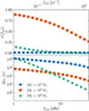 |
Fig. 1. Examples of the residence time (bottom panel), Δτc, per log10 orbital frequency bin are shown for three binaries from the HORIZON-AGN catalog, with chirp masses of 107, 108, and 109 M⊙. We also show their respective eccentricity evolution in the top panel. Eccentric systems are more efficient in dissipating the energy through GWs and this can be seen in the residence time (low panel) as compared to (nearly) circular binaries. The evolution of binaries at high frequencies (starting from a few nHz) is determined by the gravitational radiation, which is more efficient in energy dissipation for heavy and eccentric binaries. We also observe a fast circularization of eccentric systems in the top panel. |
4.2. Characterizing GW signal from a population of MBHBs
4.2.1. Properties of the GW background
The characteristic strain spectra for the circular and eccentric ensembles are shown in Fig. 2. As expected, assuming circular binaries driven by GW emission, we find a mean characteristic strain spectrum that follows the power-law behavior of Eq. (41), with an amplitude at fyr of Ayr = 3.4 × 10⁻¹⁵ and a spectral index of α = −2/3 as derived in Phinney (2001). The background amplitude for HORIZON-AGN is higher than for many other theoretical models. This can be seen in Appendix A of Agazie et al. (2023b) for pre-2023 models, as well as in new models developed by the EPTA collaboration to explain the detected amplitude (EPTA Collaboration 2024a). In fact, Izquierdo-Villalba et al. (2022) already noted that models that reproduce the background amplitude exceed electromagnetic constraints, such as the bright end of the low-redshift AGN luminosity function. In fact, HORIZON-AGN overpredicts the AGN luminosity function (Volonteri et al. 2016), explaining why the background amplitude of the simulation is closer to the value measured by PTAs compared to other models. We stress that in this paper we are not trying to “fit” the amplitude of the background, but we are trying to understand what factors influence the background, and explore the properties of the sources within a unified framework.
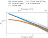 |
Fig. 2. 68% (dark) and 90% (light) confidence regions for the characteristic strain hc are shown for 2000 Universe realizations drawn from the HORIZON-AGN MBHB population, assuming either circular orbits (blue) or noncircular orbits (orange). We also plot their respective deterministic mean expectation values in dotted and dashed lines. For the circular population, we overlay as a dashed-dotted line the average spectrum, assuming the binary dynamics are driven by GW emission only. The inclusion of eccentricity introduces a significant signal reduction at frequencies lower than 10 nHz, due to the reduction of the MBHBs residence time at low orbital frequency. |
Since we included interactions with unbound stars when modeling the binary dynamics for the circular population, we did observe a slight bending of the GW spectrum at low frequencies due to the reduction of the residence time at those frequencies (Ravi et al. 2014). Overall, the bend in the HORIZON-AGN population starts to significantly affect the spectrum at observer frequencies lower than 2 nHz, which corresponds to an observation duration of around 15.8 years, in good agreement with previous studies (Sesana 2013; Kelley et al. 2017b). The current PTA experiments might already be sensitive to this effect (Chen et al. 2024).
As already demonstrated in Sesana et al. (2008) and recently investigated on the basis of PTA data in Agazie et al. (2025), the realistic Universe realization spectra from the circular population could significantly deviate from the power-law behavior with the mean spectral index corresponding to α = −2/3. This is related to the stochasticity of the GW signal from the MBHB population: it is stochastic in the limit of a large number of sources emitting in the same frequency bin during the observation period. The number of binaries per frequency bin decreases with an increase in the frequency due to the reduction in their residence time (see Fig. 1 and Eq. (29)), leading to a complete loss of stochasticity above 100–200 nHz. In the intermediate frequency range of 10–50 nHz, the decrease in the number of contributing sources increases both the variance and skewness5 of the total characteristic strain distribution across Universe realizations. This is a well-known effect, already discussed in Jaffe & Backer (2003), Sesana et al. (2008), and later elaborated in Lamb & Taylor (2024). In Fig. 2, the skewness of the strain distribution above 10 nHz is evident for the circular population, where approximately 84% of the GWB spectra have amplitudes below the square root of the average squared strain value. This renders the strain distribution at these frequencies strongly non-Gaussian. As shown in the following, this ultimately results in GWB power spectra with steeper power-law slopes compared to the average spectrum.
When eccentricity is included, we observe two main effects on the GWB spectra. First, we observe the expected bending of the GW spectrum for observer frequencies ≲ 10 nHz, significantly decreasing the background amplitude at a few nanohertz (nHz). This occurs because eccentricity spreads the GW power across multiple orbital frequency harmonics, combined with the fact that the MBHBs gradually circularize due to the emission of GW (Enoki & Nagashima 2007). The second effect of eccentricity is a slight reduction in the variance and skewness of the GW strain amplitude around fyr compared to the circular population. This is caused by the input of highly eccentric binaries with a low orbital frequency, which effectively increases the number of contributions and maintains the stochasticity at higher frequencies.
4.2.2. Properties of the contributing MBHBs
We now investigate the properties of the MBHBs that contribute the most to the GWB across the PTA frequency band. In particular, we compute the contribution of binaries to the total characteristic strain as a function of their redshift and chirp mass. We consider a PTA experiment with observation span Tobs = TEPTA ≃ 10.33 years. As mentioned above, the properties of the total characteristic GW strain vary significantly between the low and high frequency end of the PTA sensitivity band, so we take two representative frequencies: 1/TEPTA ≃ 3.1 nHz and 9/TEPTA ≃ 27.6 nHz. In Fig. 3, we show the differential contribution of the MBHB population divided into redshift slices. The solid line represents the median values across Universe realizations for each redshift slice, while the shaded region indicates the 68% confidence interval, defined here by the 16th and 84th percentiles of the distributions. At low frequencies, for circular and eccentric populations, the peak of the distribution is found around z ≃ 0.3 − 0.4. At lower redshifts, we observe a larger variance in the contribution compared to higher redshifts. Since the variance (width of the confidence interval) is primarily determined by the average number of sources contributing to the GW strain in each bin, this reflects the smaller number of MBHBs expected at low redshift. At high frequency, the peak of distribution for both populations shifts toward a higher redshift, around z ≃ 0.6 − 0.7. The heavy nearby systems, which dominate the GW signal at low frequencies, spend very little time at high frequencies; therefore, the signal accumulates over a larger volume. This also explains the very large variance compared to the low-frequency distribution: we have a lower number of binaries that contribute at high frequencies. Again, at high frequencies, the eccentric population exhibits smaller variance due to the increased number of contributing binaries. The typical redshift ranges of the MBHBs contributing to 90% of the total characteristic strain signal are given by the vertical lines in Fig. 3. These correspond to the median redshift values (across Universe realizations) at which the cumulative contribution – integrated from low and high redshifts, respectively – reaches 5% of the total strain signal. For the low frequency of 3.1 nHz considered here, where the GW signal is expected to be seen as a stochastic background, we find that most of the contribution comes from the range 0.05 < z < 1.2 for the circular population and 0.08 < z < 1.3 for the eccentric population.
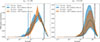 |
Fig. 3. Median and 68% confidence interval of the differential contribution to the total characteristic strain signal, based on 2000 Universe realizations, shown across MBHB redshift bins for both circular and eccentric populations. We compare the results at two observer frequencies: 3.1 nHz (left panel) and 27.6 nHz (right panel). The vertical lines represent the median redshift values at which the cumulative contribution (integrating from low and high redshifts, respectively) reaches 5% of the total strain signal for the circular (solid line) and eccentric (dashed line) populations. |
Similar distributions as a function of MBHB chirp mass are shown in Fig. 4. These distributions confirm the findings noted above. The GW signal at low frequencies is mainly formed by heavy systems with chirp mass in the range 108.5 − 109.5 M⊙, while most of the contribution at high frequencies comes from binaries in the range 108 − 109 M⊙. At low frequency, we find that the contribution to the total strain signal extends to higher masses for the eccentric population relative to the circular population. The main reason is the contribution of the massive and eccentric binaries with orbital periods around and even below the 0.5/Tobs frequency, emitting at higher orbital harmonics. The typical lower bound on the chirp mass of MBHBs contributing 90% of the total characteristic strain signal is indicated by the vertical lines in Fig. 4. These represent the median chirp mass values (across Universe realizations) at which the cumulative contribution (integrated from the lowest masses) reaches 10% of the total strain signal, for each population. We find  for the circular population and log10(ℳc/M⊙)≳8.63 for the eccentric population.
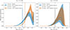 |
Fig. 4. Median and 68% confidence interval of the differential contribution to the total characteristic strain signal, based on 2000 Universe realizations, shown across MBHB log10-chirp mass bins for both circular and eccentric populations. We compare the results at two observer frequencies: 3.1 nHz (left panel) and 27.6 nHz (right panel). Vertical lines represent the median chirp mass value at which the cumulative contribution (integrating from lower masses) reaches 10% of the total strain signal for the circular (solid line) and eccentric (dashed line) populations. |
4.2.3. Number of contributing MBHBs
In this section, we aim to quantify the number of MBHBs that effectively contribute to the strain power spectrum of the GWB. This number is particularly important as it quantifies the validity of the stochasticity and Gaussianity assumption for the GWB signal in the PTA band. To estimate this number, we use two complementary metrics. The first, suggested in Bécsy et al. (2022), computes how many binary signals must be summed, starting from the brightest, to reach a fraction αtot of the total GWB power in a given observer frequency bin centered at f. This can be expressed as
 (33)
(33)
where the summation in the numerator is performed over the merger population in decreasing order of hc2. We use Eq. (30) to compute each binary’s contribution. In this analysis, we adopt αtot = 0.75, which corresponds to a S/N of 3 for the brightest sources relative to the rest of the MBHB population, defined as  .
.
However, this metric does not quantify the relative contribution of the “brightest sources”. For example, assume that 74% of the GWB power is produced by a few binaries and the remaining 1% needed to reach 75% comes from 999 MBHBs, in this case, we would obtain N75 = 1000 even though the GWs from the population are dominated by one system. To capture this potential problem, we suggest another measure, Neff, inspired by the effective sample size of a Markov Chain, derived in Elvira et al. (2022), which can be written as
![Mathematical equation: $$ \begin{aligned} N_{\rm {eff}}(f) = N_{\rm b} \frac{ \left[ \frac{1}{N_{\rm b}}\sum _l h_{\mathrm{c},l}^2(f) \right]^2}{\frac{1}{N_{\rm b}} \sum _{l} \left[h_{\mathrm{c},l}^2(f) \right]^2}, \end{aligned} $$](/articles/aa/full_html/2026/01/aa55539-25/aa55539-25-eq56.gif) (34)
(34)
where Nb is the total number of inspiralling binaries contributing to the strain signal at frequency f. One can verify that Neff equals Nb if the GW signal originates from a population of equally contributing binaries. However, if 99% of the GW signal from a population is produced by a single binary, Neff will be much closer to 1, as desired.
The (effective) number of binaries that contribute the most to the total GW strain across the PTA frequency band is presented in Fig. 5. The results for N75 are given as error boxes and median Neff values are presented by circles for the circular population and crosses for the eccentric population, for our 2000 Universe realizations. Below 10 nHz, for both populations, the typical number of binary signals that must be added to reach 75% of the background signal is greater than 300, indicating that the stochastic approximation seems justifiable at those frequencies. However, around and above fyr, for 25% of the Universe realizations, N75 is lower than 10, which is not sufficiently high to apply the central limit theorem. The eccentric background has a factor ≈10 greater number of contributors (N75) around fyr due to the distributed spectrum of GW emission and therefore maintains stochasticity to higher frequencies.
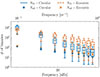 |
Fig. 5. Comparison of the effective number of binaries in terms of N75 and Neff contributing to the GWB at each observed frequency bin of a PTA with an observing duration of 10.3 years as for EPTA Collaboration (2023a). At each observer frequency, the two extreme horizontal lines represent the 5th and 95th quartiles of the N75 distribution, derived from 2000 Universe realizations. The edges and the central line of the box represent the 25th, 50th, and 75th quartiles, respectively. For Neff, we only show the median of the distribution at each observer frequency with blue dots for the circular population and orange crosses for the eccentric population. |
As the effective number of binaries, Neff, does not have a direct physical interpretation, we only compare the median values of N75 and Neff at each frequency to quantify the variation in the relative contributions of the binaries counted in N75. We find that at low frequencies, N75 is about two orders of magnitude larger than Neff for both populations. This suggests that the contribution to the total GW strain is highly uneven among binaries. In the lowest frequency bin, although around 10 000 binaries produce 75% of the background signal, only hundreds of them are significantly contributing to the signal. At frequencies below 10 nHz, even the Neff metric indicates the presence of at least tens of sources per bin, suggesting that it could be well described as a stochastic GWB.
At higher frequencies, the contributions are more balanced and point to a number of contributing binaries from a few up to several dozen binaries. This implies that at higher frequency, the background is less likely to be well approximated by a Gaussian noise and therefore is less similar to the conventional definition of a background. Taking the frequency range as a whole, one might conclude that detecting individual sources is unlikely due to the large number of contributing binaries, especially at low frequencies. However, even if the fractional contribution of an individual source is small, the cumulative effect of observing multiple pulsars within a given PTA can enhance its detectability. Furthermore, the detectability of an individual binary by a PTA must consider both pulsar noise and the detector response to GWs. This is examined in the next section, where we investigate how to pass from the properties of the strain signal to the PTA observables.
5. Implications for pulsar timing array observations
To accurately compare the theoretical signal computed from the HORIZON-AGN population with the one currently measured by PTA experiments, we must study the properties of the GWB-induced timing residuals. Timing residuals are the time difference between the measured times of arrival (ToAs) of radio pulses from Galactic millisecond pulsars and the ToAs predicted by a theoretical model, referred to as the timing model (Edwards et al. 2006). The residuals also carry an imprint from GWs; in particular, a GWB would appear as a common correlated signal with a spatial correlation pattern first derived in Hellings & Downs (1983).
5.1. Methodology
In this section we present two methods for estimating the spectral properties of the timing residuals induced by the MBHB population. We emphasize the importance of considering what affects the spectral inference of the detector (here the PTA), to avoid potential biases when interpreting its results. We also outline our methodology for identifying potentially resolvable individual binaries within the population.
5.1.1. The Gaussian ensemble approach
This approach considers the GWB signal generated by an MBHBs population as a Gaussian ensemble (see e.g., Rosado et al. 2015; Romano & Cornish 2017; Hazboun et al. 2019; Agazie et al. 2023b; EPTA Collaboration 2024a). In this case, the GW strain is considered as a random variable, fully characterized by its one-sided power spectral density (PSD), Sh(f) = hc2(f)/f. If one assumes that the GWB signal is stationary, isotropic and un-polarized, the average timing residuals response is given, in terms of PSD, by (Bertotti et al. 1983; Jenet et al. 2006)
 (35)
(35)
The timing residual PSDs from the different Universe realizations obtained using this method have two limitations. First, they do not account for the fact that the signal is produced by a discrete number of sources, each with its own response to the PTA. Second, the derivation of hc2 that leads to the timing residuals PSD  , assumes that each MBHB contributes a Dirac delta function at its orbital frequency harmonics as in Eq. (30). We recall below that this is only the case in the limit of an infinitely long dataset6. For realistic PTA data, the effect of the finite observation duration on spectral estimation needs to be considered a priori. We use a second method for evaluating
  that accounts for both of these issues in the following subsection.
5.1.2. The population approach
The principle of this approach is to compute the GWB-induced timing residuals by summing the contributions of each individual MBHB (see e.g. Bécsy et al. 2022). This requires knowledge of the waveform for any set of orbital parameters. For this approach, we consider only circular binaries.
The exact residuals induced for a given pulsar by an inspiralling MBHB depend on their relative position, the binary inclination angle ι to the line of sight and the polarization angle ψ. The time series of timing residuals is composed of two terms, corresponding to the impact of the GW strain at the time of emission of the radio pulses (referred to as the Pulsar term) and at the time of their reception (referred to as the Earth term; Detweiler 1979). The correlation between GWB timing residuals among pulsars is entirely due to the Earth term. Thus, in the following, we only consider the GW strain signal of the Earth term when computing the GWB timing residuals power spectrum. We assume GWB to be isotropic, reflecting the distribution of MBHBs across the sky. As a result, we expect the GWB to imprint, on average, the same signal in every pulsar (Hellings & Downs 1983); therefore, we compute the GWB spectrum for only one pulsar and assume that it is the same for the other pulsars in the array.
As shown in Hazboun et al. (2019), for a finite observing duration Tobs, the Fourier transform of the GW residuals induced by a circular MBHB located at a given sky position  at redshift z and emitting GW at fGW = 2forb/(1 + z) in the observer frame, takes the form
![Mathematical equation: $$ \begin{aligned} \tilde{r}_{\rm GW}(f) = R_0 \left[ G_{\hat{k}} e^{i\phi _0}\delta _{{T_{\rm {obs}}}}(f - {f_{\mathrm{GW} }}) + G_{\hat{k}}^*e^{-i\phi _0} \delta _{{T_{\rm {obs}}}}(f + {f_{\mathrm{GW} }}) \right], \end{aligned} $$](/articles/aa/full_html/2026/01/aa55539-25/aa55539-25-eq61.gif) (36)
(36)
where ϕ0 is an (arbitrary) initial GW phase and the amplitude R0 depends on the intrinsic properties of the binary:
 (37)
(37)
where we introduced the redshifted chirp mass ℳc, z = (1 + z)ℳc. The residuals amplitude is modulated by the complex geometric factor  given as
![Mathematical equation: $$ \begin{aligned} G_{\hat{k}} = -\frac{1}{2}\left[\cos \iota F^\times (\hat{k}, \psi )+i\frac{1 + \cos ^2\iota }{2}F^+(\hat{k}, \psi ) \right], \end{aligned} $$](/articles/aa/full_html/2026/01/aa55539-25/aa55539-25-eq64.gif) (38)
(38)
where we introduced the antenna pattern response function for both + and × polarization modes that depends on the sky position of the pulsar and binary as well as on the polarization angle ψ. Their exact expressions can be found in Ellis et al. (2012). Finally, we must correctly take into account the finite duration of the PTA observations (Tobs) by introducing the edge effect into the Dirac delta function:
 (39)
(39)
Contrary to the previous case where we considered Dirac delta functions as a contribution of each MBHB, the finite width of the sinc function leads to spectral leakage in the non-white PSD. As a result, every MBHB can potentially contribute to several frequencies, which makes frequency bins correlated. It is common practice in signal processing to taper the time series to minimize the effect of spectral leakage (Percival & Walden 1993). However, in current PTA data analysis, no such pre-processing is applied to the timing residuals time series, so it might, a priori, affects the inference of the PSD. This suggests that even MBHBs emitting GWs at frequencies much lower than the PTA frequency (1/Tobs) could contribute to the GWB power inferred in the PTA band due to spectral leakage.
The spectral leakage could (at least partially) be mitigated by the timing model. A part of the timing model fits and removes linear and quadratic trends in the PTA residuals that could be caused by the spin-down in the millisecond pulsars. Obviously, it also removes some very low-frequency GWs covariant with such a trend (Cordes & Shannon 2010; van Haasteren & Levin 2013). As a result, it can significantly reduce the dynamical range in the expected PSD and decrease the effect of spectral leakage. An effect already discussed in Taylor et al. (2013), Lentati et al. (2013). However, the timing model cannot be a replacement for a well-designed taper that controls the leakage. Nonetheless, the timing model acts as a high-pass filter that removes very low-frequency GWB (≲1/Tobs) from the pulsar timing residuals (Hazboun et al. 2019). As a result, we consider only MBHBs that emit GWs with fGW > 1/(2Tobs) in order to reduce the numerical cost of the GWB computation without affecting its inferred properties in the PTA frequency band.
We produce realistic GWB timing residuals by summing the contributions from all MBHBs of a given Universe realization, uniformly drawing the sky location, polarization angle, and initial phase for each binary. However, since the number of MBHBs contributing to the PTA band typically exceeds millions, we employed a numerical simplification, which allowed us to carry out this procedure more efficiently; the procedure is described in Appendix B. Once the GWB timing residuals waveform  is obtained, we can return to the time domain and infer the GWB PSD using the data analysis procedure commonly employed in the PTA community. In the following, we briefly discuss the PSD inference procedure used for PTA data.
5.1.3. The GWB spectral inference in PTA
The GWB analysis performed by PTA collaborations is based on the modeling of the timing residuals data (intrinsic red noise, dispersion measure variations, GWB, etc.) using Gaussian processes. Each noise component X is modeled using a truncated Fourier basis where the  coefficients
  , are distributed according to a multivariate Gaussian with a covariance matrix reflecting the underlying process, characterized by its PSD
  :
:
 (40)
(40)
This defines a prior for the noise Fourier coefficients, that depends on some parameters θX, which characterize the PSD of the process. It is then usual procedure to marginalize over these coefficients so that the PTA likelihood depends only on the PSD parameters θX (Lentati et al. 2013; van Haasteren & Vallisneri 2014). The observation time Tobs, in Eq. (40), is defined depending on whether the noise component, X, is intrinsic to a specific pulsar or not. If it is intrinsic, Tobs is the observation duration of that pulsar. If X is a common process, such as a GWB, Tobs is the total observation duration of the PTA.
There are two main methods for inferring the timing residuals PSD, Sr(f). The first introduces the parametrized description resulting from a particular physical model. For example, the population of inspiralling binaries should produce a characteristic strain described by a power law (Phinney 2001):
 (41)
(41)
which implies a power-law form  for the timing residuals PSD with γ = 3 − 2α, using Eq. (35). The spectral index γ and an amplitude at fiducial frequency fyr = 1/yr are inferred from the data using a Bayesian framework. This requires a choice of prior for the GWB parameters θGWB = (Ayr,γ). We use a log-uniform prior for the GWB amplitude, log10Ayr ∈ [ − 18, −10] and a uniform prior for its spectral index, γ ∈ [0, 7].
In the second approach, often referred to as “free spectrum”, we infer directly the values Sr(fk) at a set of harmonics fk = k/Tobs assuming that they are independent (Lentati et al. 2013; Taylor et al. 2013). More specifically, the inferred quantities are the residuals root-mean-square (RMS),  . Here, we only sample the RMS coefficients up to fyr, choosing a log-uniform prior for each
 ![Mathematical equation: $ \log_{10} \left({\rho_{\mathrm{r}}^{(\mathrm{GWB})}}(f_k) / \text{ s}\right)\in [-10, -4] $](/articles/aa/full_html/2026/01/aa55539-25/aa55539-25-eq74.gif) . This method is model-agnostic, but constrained by the assumption of independence of estimate at each frequency bin. Given the current poor sensitivity of PTAs, both approaches give a consistent estimate of the signal PSD (see Agazie et al. 2024).
. This method is model-agnostic, but constrained by the assumption of independence of estimate at each frequency bin. Given the current poor sensitivity of PTAs, both approaches give a consistent estimate of the signal PSD (see Agazie et al. 2024).
In the following, we apply this PTA Bayesian spectral estimation method to the GWB-induced timing residuals of a single pulsar, obtained using the population approach described above. Since we are only interested in the accuracy of the spectral inference and its potential limitations (e.g., regarding spectral leakage), we simplify simulated PTA data and include/consider only white noise residuals in addition to the GWB timing residuals associated with each Universe realization7.
5.1.4. Searching for bright individual binaries
In the previous sections, we refer to the GW signal from the MBHB population as a GWB. However, the population modeling approach emphasizes that the signal is, in reality, a sum of individual sources. As a result, it could be that the GW signal consists of a few resolvable bright binaries, referred to as continuous wave (CW) in the following, on top of the stochastic GWB (Sesana et al. 2008). To quantify the potential detectability of individual sources, we evaluate the S/N of the brightest binaries for our 2000 Universe realizations, using two toy PTA datasets. We then consider a CW with an S/N greater than 3 as a potentially detectable individual binary. This calculation applies only to the population modeling, and thus, for this study, to the circular ensemble.
We identify the CW candidates as follows. First, for each Universe realization, we obtain a list of potential CW candidates by identifying the individual binaries with the highest residuals amplitude R0 across a frequency grid covering the PTA sensitivity band. For each of these brightest candidates, we then compute the associated GWB ‘noise’ excluding the CW candidate waveform,  . We then apply a Hanning window function wHanning to limit spectral leakage (Harris 1978) and then compute its periodogram to estimate its PSD. This effectively gives
 (42)
(42)
The obtained GWB noise PSD is used to compute the CW candidate optimal match filtering S/N (see e.g., Creighton & Anderson 2011) for the PTA with a noise covariance matrix, CPTA, as
 (43)
(43)
where the CW residuals vector rCW is the concatenation of the CW residuals for the different pulsars of the PTA. The noise covariance matrix CPTA of the PTA is constructed using the enterprise software (Ellis et al. 2020). The noise matrix contains four contributions. The first one is the result of the timing model marginalization (TMM) procedure and can be seen as a transmission function reducing the sensitivity at low frequencies and removing 1/year frequency from the analysis (see discussion above and Hazboun et al. 2019). The second contribution is an intrinsic timing red noise component for each pulsar of the PTA with a PSD modeled as a power law,  . We set log10Ayr = −13.5 and γiRN = 3, for all the pulsars of our toy PTAs; this corresponds to the typical noise process properties found in EPTA Collaboration (2023b). The third component is the white noise characterized by
  , where (i) σPTA is the typical residuals RMS due to the radio telescope noise and pulse jitter (Shannon & Cordes 2012) defined above (ii) Δtobs is the observation cadence, which we assume to be constant and equal across pulsars. Finally, we include the GWB, which is correlated among pulsars, using Eq. (42) and the Hellings-Downs correlation function (Hellings & Downs 1983). We note that this assumes that the GWB noise PSD is the same for all the pulsars in the toy PTA, which is a reasonable assumption for an isotropic stochastic background.
The simulated PTAs and noise parameters are given in Table 1. The EPTA configuration is based on the properties of the EPTA DR2new dataset presented in EPTA Collaboration (2023c), while the SKA represents an expected configuration of the future SKA dataset (Janssen et al. 2015), choosing a similar observation duration as for EPTA. For each toy PTA and each Universe realization, we randomly assign sky positions to pulsars, uniformly distributed across the sky, and draw their distances from Earth from a normal distribution with a mean of 1 kpc and a standard deviation of 0.1 kpc. Assuming an isotropic pulsar distribution reduces the dependence of the detectability of a CW candidate on the pulsars’ positions and distances.
Configuration of the two toy PTAs used to infer the detectability of individual MBH binary.
5.2. Results
5.2.1. Comparison with EPTA results
We now examine the properties of the timing residuals induced by the GW signal from our MBHB population. We compare our theoretical expectations, based on the Gaussian ensemble (GE) and population approaches described above, with the current EPTA results obtained with the DR2new dataset, which includes residuals from 25 millisecond pulsars observed over a duration of TEPTA ≃ 10.3 years (EPTA Collaboration 2023c). PTA collaborations are providing the estimated residuals PSD using a power law and a free spectrum model. For the population approach, we compare the GWB spectral inference with and without the TMM procedure described above to quantify its performance on reducing spectral leakage effects.
Our comparison for the power-law PSD model is shown in Fig. 6, where the EPTA results are shown as red dotted lines in both panels. The results using the GE approach are given in the left panel. We show the power-law parameters obtained from a least-squares fit using a power law (assuming Eq. (41) and using Eq. (35)) on the PSD produced by the population for each of the 2000 Universe realizations. We apply the same weight to each observer frequency fk for the least-squares fit. For the population approach, we combine the maximum-a-posteriori samples obtained from the PTA Bayesian spectral inference (using a power-law PSD model) on the timing residuals derived from our 2000 Universe realizations.
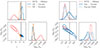 |
Fig. 6. Distributions of the amplitude Ayr at fyr and the spectral index γ, which parameterize the GWB timing residuals PSD, derived from 2000 Universe realizations, are compared with the EPTA results (red dotted contours) of EPTA Collaboration (2023a). The 68% and 90% confidence regions are shown for all distributions. Left panel: Distributions obtained via power-law least-squares fits to spectra from the Gaussian ensemble (GE) method for the circular (blue) and eccentric (orange) populations are shown as filled contours. Right panel: Distributions of maximum-a-posteriori power-law parameters from PTA-like inference using the GWB timing residuals from the population (Pop) approach. Solid contours represent the standard data analysis procedure that includes TMM; dashed contours represent the analysis without TMM. The effects of spectral leakage on the inference are clearly visible without TMM and remain measurable even when TMM is included. In both panels, the expected spectral index, γ = 13/3, of the average spectrum from a population of circular binaries driven by GW emission, is shown as a black vertical line. Note: γ relates to the characteristic strain spectral index α via γ = 3 − 2α. |
Using the GE approach, we find that circular MBHBs would induce a slightly steeper residual PSD than expected from the Phinney average power law, γ = 13/3 ≃ 4.33 (α = −2/3 in terms of hc), with a 90% confidence interval of  . For the associated characteristic strain at fyr, we find
  . The eccentric population produces shallower spectra with a 90% confidence interval of
  , and induces a similar amplitude at fyr, of
  . For circular and eccentric ensembles, when using the GE approach, we recover a background that is steeper and fainter (at fyr) compared to the observations from the EPTA.
We compare results using the population approach and the PTA Bayesian spectral inference method in the right panel of Fig. 6. First, as shown by the blue solid contours, the PTA inference which includes TMM leads to a distribution of power-law parameters that is much broader than the GE approach. This is expected because the population approach accounts for both the realistic pulsar response to binary signals – which reduces the effective number of binaries contributing to the pulsar timing residuals – and the limited sensitivity of the PTA, unlike the GE approach. We find 90% confidence intervals of  and
and  for our 2000 Universe realizations. The extension of the spectral index posterior toward lower values, around 3, along with an increase in the background amplitude at fyr, is likely due to residual spectral leakage effects.
Let us say a few more words about the importance of spectral leakage in the inference of the GWB. The dashed blue contours give the posterior distribution of the inferred GWB spectra without TMM. As mentioned above, TMM works as a kind of low-pass filter, which reduces the spectral dynamical range and, therefore, reduces the leakage. The effect of GWB spectral leakage is obvious in this case: the posterior is significantly biased toward higher amplitudes and shallower spectra, with a 90% confidence interval  and
and  . If spectral leakage is improperly handled, each individual binary, as expressed in Eq. (36), contributes to the GWB spectral inference with a decaying tail ∝1/f2 at high frequencies. As a consequence, the more massive (and more numerous) binaries orbiting at low frequencies artificially contribute to the GWB spectrum at much higher frequencies than their actual GW frequency. Although the TMM procedure significantly filters out low-frequency contribution it does not eliminate the leakage completely, which still contributes to the shallower spectra part of the posterior depicted by the solid line. We note that this effect is more evident for the more sensitive SKA toy PTA, where we find a 90% confidence interval of
  . The asymmetry in the confidence interval toward shallower spectra is highlighting the impact of spectral leakage on the PTA spectral inference, even when the TMM is included8. Both the increase in amplitude at fyr and the decrease in spectral index induced by spectral leakage tend to align the inferred properties of the GWB signal from the HORIZON-AGN MBHB population with EPTA observations. We claim that this should be further investigated as a potential bias in the PTA spectral inference pipeline.
To have a more comprehensive view of what is happening across the PTA band, we compare our results with observations, using the model-agnostic free spectrum approach for the residuals PSD. The results are presented in Fig. 7. For clarity and because the spectral uncertainties are much smaller for the GE approach, we show only the average spectrum for the circular (solid blue line) and eccentric (dashed orange line) ensembles, omitting their corresponding confidence regions. The spectrum produced by the circular population is slightly steeper than the free spectrum suggests, while the eccentric population better fits the observed EPTA free spectrum (red violins). For the population approach, we evaluated the free spectrum with (dashed blue violins) and without TMM (solid light blue violins). The analysis without TMM again clearly exhibits the spectral leakage at high frequencies as a flattening tail. And once again, we do observe that TMM does not completely eliminate the leakage in some Universe realizations. This remains a concern, as overestimating the GWB amplitude at fyr can skew the astrophysical interpretation of the signal.
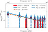 |
Fig. 7. Comparison of the GW residuals RMS induced by the HORIZON-AGN population, using different modeling and populations, with the spectrum measured by the EPTA collaboration, shown in red. The average GE spectra of both circular and eccentric ensembles are depicted as solid and dashed lines, respectively. The distribution of the maximum-a-posteriori samples for the GWB spectra of the 2000 Universe realizations obtained using the population (Pop) method and a realistic PTA-like inference with and without TMM, are shown in dashed contours and light blue color, respectively, for the circular population. The effect of spectral leakage on the GWB inference results in a shallower spectral shape, significantly biasing the inference when TMM is not included. For some Universe realizations, spectral leakage still has appreciable effects at high frequencies even when TMM is applied. |
5.2.2. Likelihood of individually resolvable binaries
Using the method described in Sect. 5.1.4, we go on to assess the presence of binaries with an S/N greater than 3. We refer to these as CW candidates, attributed to each of our 2000 Universe realizations and for the two toy PTAs.
The results are summarized in Fig. 8, where we group the CW candidates by their GW frequency in the observer frame. Overall, we find that the toy EPTA (resp. SKA) experiment has at least one CW candidate in approximately9 4% (resp. 20%) of our Universe realizations. For EPTA, there is a 4% probability of having one and a 0.1% probability of having two CWs with S/N > 3 across the frequency band. For the SKA, we find probabilities of 18%, 2%, and 0.3% for having 1, 2, and 3 CW candidates, respectively. These candidates are predominantly found in a frequency range between the lowest frequency of PTA, 1/Tobs, and a few times this frequency. Indeed, at lower GW frequencies, CW candidates compete with a greater number of binaries and are also affected by the timing model. On the other hand, bright CW sources at higher frequencies are also rare, as massive binaries evolve fast and are unlikely to be found at these frequencies, as shown earlier. Furthermore, due to white noise and the PTA response to the GW signal, the sensitivity drops significantly at higher frequencies (Hazboun et al. 2019). These findings are in agreement with previous studies (Rosado et al. 2015; Bécsy et al. 2022). However, we note that the probabilities we obtain are only lower bounds for the presence of CW candidates because our criteria for selecting CW candidates before computing their S/N are not optimal, as they do not account for the geometry of the PTA. As a result, the MBHB with the highest residual amplitude R0 may not be the one that maximizes the S/N for a particular PTA configuration.
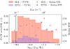 |
Fig. 8. Probability of detecting a Continuous Wave (CW) signal from an individual MBH binary with a GW frequency in a given range, with an S/N greater than 3 for two toy PTAs representing the EPTA and the future SKA. Probabilities, shown as histograms, are derived from 2000 Universe realizations. The medians of the S/N distributions in each GW frequency band are overlaid, shown with dots (EPTA) and crosses (SKA). The frequency associated with the observation duration of the PTAs (10.33 years) is shown as a black vertical line. |
In Fig. 8, we analyze the dependence of the median S/N of these CW candidates on their GW frequency. The median values in the frequency bins associated with a probability below 1% are not statistically robust, as they include fewer than 20 CW candidates with S/N > 3 and thus could be subject to significant variance. Therefore, based on the SKA results, we find that the median S/N tends to increase with the GW frequency of the CW candidate, in agreement with previous findings (EPTA Collaboration 2024a). The properties of these CW candidates will be investigated in the next sections, along with the electromagnetic properties of their host galaxies.
6. Properties of MBHs and host galaxies
Based on the analysis presented in the previous sections, here we focus on binaries with chirp mass > 108.35 M⊙ and 0.05 < z < 1.2 as the dominant component of the background (Sect. 4.2.2) and the selected individual CW candidates in population modeling for circular binaries (Sect. 5.2.2) as representative of the population. As a general point of information, a given MBH may appear in the catalog multiple times with multiple redshifts as it merges with different MBHs. This is the case for the most massive MBHs, hosted in very massive galaxies, since they experience numerous mergers in their lifetime. Physically, this does not mean that a given binary in the Universe would be detected multiple times. However, if a simulation is a realistic representation (of a finite volume) of our Universe, the MBH binaries populating a given redshift layer will have similar properties as those merging at the corresponding redshift in the simulation. For a sufficiently large simulation box, which probes the large scale structure of the Universe, this is a reasonable assumption.
First, we consider what it is that makes an MBHB a good CW candidate physically. Besides its position in the sky, near pulsars, and its inclination, which we assumed to be both random in our analysis, the only physical quantities from the simulation are chirp mass and redshift. We consider binaries that make the best CW candidates as those that appear most often in the various Universe realizations. The best CW candidates are not necessarily those that have the largest S/Ns. The largest S/Ns are obtained for the largest chirp masses and the lowest redshifts (luminosity distance). The largest chirp masses have however the shortest residence times in the PTA band (Mingarelli et al. 2017), making it harder to catch them in the act. The lowest redshift sources are rarer because of the small volume probed. As a result, the binaries associated with the very high S/N are also appearing very rarely in the Universe realizations. We therefore consider as “high probability” CW candidates those that appear multiple times (i.e., at least five times in this work) across our 2000 realizations.
In the following, we consider both the simulation box, which is an evolving patch of the Universe that we can analyze at different times, and the simulation lightcone, which mimics what and how an observational survey would “see” the simulation. When we move from the simulation box to the lightcone generated for the simulation (Laigle et al. 2019) a given MBH appears only once, and the cosmic time at which the MBH appears in the lightcone may or may not coincide with the time of an MBH merger. This means that only a small fraction of merging binaries are contained in the lightcone.
In Fig. 9, we compare the properties of mergers dominating the background in the simulation box which has a fixed co-moving volume (teal), in the simulation lightcone (light green) which simulates the source distribution seen by an observer, and the CW candidates (red). In these distributions, we include CW candidates accounting for their multiplicity across Universe realizations, as the multiplicity of a given candidate in the various realizations provides information on how strong a candidate is as it provides information on its likelihood. In a cosmological volume, and in a lightcone that has increasing volume as redshift increases, the background is dominated by the more abundant MBHs with mass ∼108.5 M⊙, rather than the stronger but rarer GW sources with larger mass. CW candidates are instead mainly found at low redshift and have higher MBH masses; some can also have relatively low masses, down to ∼3 × 10⁷ M⊙, but they are all at z < 0.1. The redshift distribution extends to higher redshifts in the lightcone, because of the larger volume probed with increasing redshift, while it is limited to lower redshifts for CW candidates, because the strength of the GW signal decreases with increasing luminosity distance, hence redshift. The degeneracy between luminosity distance (redshift) and chirp mass (see Eqs. (22) and (30)) allows for the presence of CW candidates up to z = 0.4, provided that they have chirp mass ℳc ∼ 109.5 M⊙. The distribution of the masses of the host galaxies reflects the ℳc and z distributions for the background, while for CW candidates it is dominated by massive galaxies, in line with the larger MBH masses with respect to the background. These results are in agreement with previous and concurrent investigations (e.g., Sesana et al. 2009; Cella et al. 2025; Truant et al. 2025).
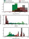 |
Fig. 9. Properties of MBH binaries and their host galaxies, for systems dominating the background and CW candidates. From top to bottom, we show distributions of chirp mass, redshift and stellar mass of the host galaxy. The teal dotted histogram shows the distribution in the box volume (140 cMpc)3, the green histogram shows the simulation lightcone that models the galaxy distribution as seen by an observer, while the red hatched histogram shows CW candidates (‘CW cand’), with the gray histogram highlighting the high probability ones. In these distributions, we include CW candidates accounting for their multiplicity across Universe realizations. |
We examine the relation between binaries and environment in Fig. 10. Here, ℳc is shown as a function of the halo mass of the host. We note some “undermassive binaries,” with very low chirp mass with respect to the host galaxy/halo: these are cases where the mass ratio in the binary is very small, and therefore the chirp mass differs significantly from the binary mass, which is what scales with host properties in the simulation (shown in Volonteri et al. 2020). The binaries dominating the background in the simulation box are primarily hosted in galaxies and halos that are more massive than the Milky Way, while CW candidates are, for the most part, hosted in group-like main halos (red squares) with Mhalo > 1013 M⊙. CW candidates that are hosted in lower mass halos are all located in subhalos (orange crosses), meaning that the subhalo has been affected by stripping and it is part of a larger halo;10 the high chirp mass with respect to halo mass is explained by stripping of the halo, which has therefore lost part of its mass (see the discussion in Volonteri et al. 2016, for the general MBH population). This implies that CW candidates are best looked for in galaxy groups and clusters, even more so than for the general population of MBH binaries (Rosado & Sesana 2014; Izquierdo-Villalba et al. 2023; Saeedzadeh et al. 2024). Using groups/clusters as priors for where to look for CW candidates in the Bayesian search of PTA data could be therefore a possible strategy.
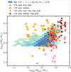 |
Fig. 10. Environmental properties of MBH binaries and their host galaxies, for systems dominating the background (bck) and CW candidates (CW cand). From top to bottom, we show the chirp mass as a function of the stellar mass of the host galaxy and of the mass of the halo hosting the galaxy. Binaries hosted in central halos are shown as red squares; binaries hosted in subhalos are shown as orange crosses. An inner black marking highlights the high probability CW candidates. |
Furthermore, the MBHs in the central galaxies of overdensities experience a large number of mergers, up to ∼20 − 25 for the MBHBs that dominate the nHz background. This is a manifestation of the significant fraction of MBH mass gained through MBH mergers for these galaxies (Volonteri & Ciotti 2013; Dubois et al. 2014b; Kulier et al. 2015). This occurs because of a combination of enhanced galaxy mergers and decreased gas availability for accretion for high-mass MBHs hosted in massive central galaxies of groups and clusters.
In Fig. 11, we compare the Eddington ratios and star formation rate (SFR) of background sources in the box vs CW candidates. We average SFR over 100 Myr since most star formation diagnostics probe SFR on such timescales and we average fEdd over 1 Myr to smooth the variability. Also in this case we include CW candidates accounting for their multiplicity across Universe realizations. The Eddington ratio of the binaries is generally low, < 10−2, typical for MBHs of this mass and redshift in the simulation as well as in observations (Volonteri et al. 2016). Accretion is even lower for CW candidates, since they are at very low redshift, in very massive galaxies. The same considerations apply to SFR, in agreement with previous results which find that the host has low SFR or specific SFR (Saeedzadeh et al. 2024; Truant et al. 2025; Cella et al. 2025). Since we are considering delayed mergers rather than numerical mergers, the time elapsed from galaxy merger to binary observation is sufficiently long that any galaxy merger-driven increase in accretion rate or SFR has since decayed (Dong-Páez et al. 2023).
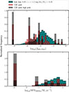 |
Fig. 11. Properties of MBH binaries and their host galaxies, for systems dominating the background and CW candidates. Top: Eddington ratio of the binary averaged over 1 Myr around the time when the MBHs merge. Bottom: SFR averaged over 100 Myr. The teal dotted histogram shows the MBHBs dominating the background, selected in the simulation box. The red-hatched histogram shows CW candidates, with the gray histogram highlighting the high probability ones. MBHs with fEdd = 0 are shown at fEdd = 10−8 and galaxies with SFR = 100 Myr = 0 are shown at SFR = 100 Myr = 10−3. In these distributions we include CW candidates accounting for their multiplicity across Universe realizations. |
Examples of hosts of CW candidates in false gri colors are shown in Fig. 12 and Fig. 13. The MBHB is located at the center of the image. The first three images (Fig. 12 and Fig. 13 left) show two low-redshift cases consistently appearing in the realizations, while Fig. 13, right, shows a rarer high-redshift (z = 0.42) case. The images highlight that CW candidates are preferentially found in the center of galaxy groups and clusters, in agreement with the results shown in Fig. 10.
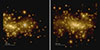 |
Fig. 12. Left: Environment of a CW candidate binary with log10(ℳc/M⊙) = 9.02 and total mass log10(MBH/M⊙) = 9.97 at z = 0.025, hosted in a galaxy with log10(M★/M⊙) = 12.19 in a halo of mass log10(Mhalo/M⊙) = 13.44. Right: Environment of a CW candidate binary with log10(ℳc/M⊙) = 9.55 and total mass log10(MBH/M⊙) = 10.04 at z = 0.026, hosted in a galaxy with log10(M★/M⊙) = 12.69 in a halo of mass log10(Mhalo/M⊙) = 14.70. |
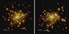 |
Fig. 13. Left: Environment of a CW candidate binary with log10(ℳc/M⊙) = 9.07 and total mass log10(MBH/M⊙) = 10.16 at z = 0.032, hosted in a galaxy with log10(M★/M⊙) = 12.48 in a halo of mass log10(Mhalo/M⊙) = 14.44. Right: Environment of a CW candidate binary with log10(ℳc/M⊙) = 9.57 and total mass log10(MBH/M⊙) = 10.06 at z = 0.42, hosted in a galaxy with log10(M★/M⊙) = 12.40 in a halo of mass log10(Mhalo/M⊙) = 14.30. This is one of the highest redshift CW candidates in our analysis, and it is the progenitor of the MBH shown at later redshift in the left panel. |
7. Electromagnetic emission from galaxies and MBHs
7.1. Methodology
In this paper we do not model specific binary signatures and we instead focus on the sheer detectability of AGN and host galaxies, addressing two points. The first is whether the galaxy/AGN are within the reach of observational surveys. The second is whether the AGN emission can outshine the emission from the host galaxy.
Galaxies magnitudes are computed as described in Laigle et al. (2019). In brief, we compute the galaxy rest-frame spectral energy distribution by summing up the contribution of all stellar particles (knowing their ages and metallicities), assumed to behave as single stellar populations. We use the stellar population synthesis model of Bruzual & Charlot (2003) assuming a Chabrier (2003) initial mass function. The dust column density and optical depth along the line of sight of each star particle is computed assuming that 30% of metals in the galaxy gas distribution are locked into dust grains. We use the RV = 3.1 Milky Way dust grain model by Weingartner & Draine (2001). Apparent total magnitudes are computed on the redshifted spectra, using the B, V and Ks filters.
In X-rays, the galaxy emission is dominated by X-ray binaries composed of a compact object accreting from a companion star. Empirical models allow for the combined effect of low-mass X-ray binaries to be estimated, where the companion is a low-mass star and the emission depends on the total galaxy mass, and high-mass X-ray binaries, where the companion is a high-mass star and the emission depends on the SFR. These models are based either on individual observations of nearby galaxies (e.g., < 50 Mpc, Lehmer et al. 2019) or on stacked galaxies observed up to high redshift (Fornasini et al. 2018, z < 5). We calculate the combined X-ray luminosity of X-ray binaries in galaxies using the relations of Fornasini et al. (2018).
We further estimate the radio emission from stellar populations in galaxies based on the relation between SFR and radio luminosity derived by Bell (2003). This relation fits SFR as a function of radio luminosity, rather than vice versa, which is what we need. Garn et al. (2009), however, show that the relation provides a good fit to radio luminosity as a function of SFR. We therefore simply invert the equation to obtain radio luminosity as a function of SFR.
We model the emission from MBHs by considering the total mass of the binary and the accretion rate recorded in the simulation averaged over 1 Myr around the time when the MBHs merge. This is to account for that the MBHs can be observed at any point during the time spent in band, and this time is generally of the order of a Myr (see Fig. 1).
We model the AGN emission from X-ray to infrared (IR) using the average spectral energy distribution for AGN developed in Shen et al. (2020). We add a correction for dust by estimating the hydrogen column density within a sphere of radius 4 kpc, assuming a dust-to-gas mass ratio of 10−2 and a Milky Way-like extinction curve. For simplicity we fit the hydrogen column density for the MBH population as
![Mathematical equation: $$ \begin{aligned} \log _{10}\left(\frac{N_{\rm H}}{\mathrm{{cm}^{-2}}}\right) = 22.54-0.23(1+z)+[0.65-0.1(1+z)]\log _{10}(f_{\rm {Edd}}), \end{aligned} $$](/articles/aa/full_html/2026/01/aa55539-25/aa55539-25-eq89.gif) (44)
(44)
and then apply this scaling to the binaries.
The AGN radio luminosity is calculated via the fundamental plane of black hole accretion, an empirical correlation between the MBH mass, the radio and X-ray power-law continuum luminosities (Gültekin et al. 2019, note that this is the core radio luminosity and not the total luminosity including extended jets):
 (45)
(45)
where LR, 5 is the radio luminosity at 5 GHz (rest frame), and LX is the X-ray luminosity in the rest-frame 2−10 keV energy range, both in erg s−1. Radio luminosity is calculated at 2 GHz (observer frame), assuming a power-law spectrum with index −0.7 (Gültekin et al. 2014).
We should mention important caveats. For MBHs with Eddington ratio ≲10−2 − 10−3, the total luminosity should be rescaled to account for radiatively inefficient accretion discs, and the spectral energy distribution differs overall from the radiatively efficient case. We compared the results with the specific radiatively inefficient solution developed by Nemmen et al. (2014) for a range of masses and accretion rates, and found that rescaling the X-ray to IR spectral energy distribution by a factor fEdd (Merloni & Heinz 2008) gives an estimate within a factor of about 5 from the Nemmen et al. (2014) solution. Given the large uncertainties, we report the radiatively inefficient sources, which we define as having fEdd < 10−3, with an optimistic estimate corresponding to the radiatively efficient case, and we discuss the case corresponding to the same multiplied by fEdd to assess the effect of suppressing the radiative efficiency.
7.2. Electromagnetic properties of MBHs and host galaxies
We compare the brightness of CW candidates and their host galaxies in Fig. 14. The host galaxies are shown as black empty pentagons and the AGN as red filled dots for fEdd > 10−3 and as orange triangles otherwise, optimistically assuming radiatively efficient accretion even at low Eddington ratios. Appendix C compares with radiatively inefficient accretion.
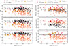 |
Fig. 14. Electromagnetic properties of MBHBs and their host galaxies for CW candidates. The left panels show B, V, and K magnitudes; the right panels show X-ray flux at [2–10] keV, radio flux at 2 GHz and bolometric luminosity (the horizontal line marks Lbol = 1045 erg s−1), as a typical value for quasar luminosities. For MBHs with fEdd < 10−3 we show an optimistic upper limit to the brightness ignoring the correction to radiative efficiency. |
The first point to note is that the large majority of MBHBs have bolometric luminosities below 1045 erg s−1, the typical dividing line between quasars (brighter sources) and AGN (fainter sources). This is because, although the MBHs are very massive, their typical accretion rates are very low (Fig. 11). Only 9% of CW candidates, and 16% of the high probability CW candidates, have Lbol > 1045 erg s−1. More generally, the electromagnetic properties of the CW candidates are very similar to those of high-probability CW candidates. The fraction is about 3% for MBHBs dominating the background (see Appendix C). This is in agreement with Truant et al. (2025). A related, but slightly different question, is the binary fraction in quasars. The fraction of quasars with Lbol > 1045 erg s−1 that host binaries close to coalescence – without a restriction to nHz frequencies – is 7% in our model. Casey-Clyde et al. (2025) also find a low binary fraction in quasars (∼4%).
In the optical and near-IR (NIR) bands (B, V, and K) the host galaxies are generally bright, with magnitudes brighter than 20, while about half of the AGN have magnitudes fainter than 20. The results are in qualitative agreement with Veronesi et al. (2025), although we do not find a similarly strong dependence of the photometric properties of the binary and its host on the binary mass. Even in this optimistic scenario for the radiative efficiency, none of the MBHBs with fEdd < 10−3 are brighter than the host galaxies, while for MBHBs with higher accretion rates, 34%, 17% and 26% are brighter than the host in B, V, and K respectively. In radio and X-rays, all MBHBs with fEdd > 10−3 are brighter than the host, while the low accretors can be outshined by the stellar emission from the host galaxy. If we optimistically do not include a correction for radiative inefficiency, about 30% (X-ray) and 80% (radio) can be brighter than the host. Results are qualitatively similar for binaries dominating the background. In Appendix C, we explicitly show the ratio of AGN and host galaxy luminosity for this optimistic case as well as the results when applying a correction for radiatively inefficient sources. Figure C.2 highlights how MBHBs with fEdd < 10−3, which are the majority of the sample, are in the more pessimistic case always fainter than the galaxy emission, even in X-ray and radio. Overall, however, we consider the radio band the best suited for identifying MBHBs with less contamination from the host galaxy, followed by X-rays.
The preponderance of faint AGN outshined by their host galaxies among CW candidates makes searches for MBHBs harder: variations of the MBHB light curve have to be extracted from the brighter nonvariable (unless there is a rare event like a supernova) galaxy emission. Electromagnetic searches for MBHBs are therefore often limited to the brightest MBHBs, which are however a minority with respect to the full MBHB population. For instance, Foustoul et al. (2025) searched for MBHB candidates, looking for continuous periodic modulation in the optical light curves (g- and r-bands) of sources coincident with the centers of galaxies. Each candidate found in Foustoul et al. (2025) was shown to be a quasar and the luminosity of the central MBHB candidate outshines the host galaxy. Plotted in Fig. 14 are the electromagnetic properties of these MBHB candidates at redshift 0.4 < z < 1.0. We show all candidates for which there are K-, V- and B-band photometry (left-hand plots) or X-ray detections/upper limits (right-hand plots). Considering an orbital origin for the optical variability, the separation of these candidates is between 4 and 13 mpc, similar to those in the simulations and making them potential PTA CW sources. We calculated their chirp mass, shown in Fig. 14, supposing an equal mass binary and with masses estimated from their SDSS optical spectrum in Rakshit et al. (2020). The bolometric luminosities were estimated using their X-ray detections/upper limits and the bolometric correction computed for type I AGN in Duras et al. (2020). The MBHB candidates have B, V, and K magnitudes slightly fainter than many of the galaxies and AGN in Fig. 14 as they are on average at greater distances than the CW candidates in the simulation. The X-ray fluxes are similar to the CW candidates, but again slightly fainter than the AGN due to the greater distances. Accounting for distance (redshift) by considering the X-ray luminosity, the electromagnetic candidates show very similar luminosities as the AGN and indeed all of them are quasars (see also Foustoul et al. 2025). Calculating the Eddington ratios for the MBHB candidates, we determined ratio values between 0.05 and 0.3, indicating high accretion rates that would explain the high bolometric luminosities for these candidates. Overall, the electromagnetic properties of the MBHB candidates are similar to the expected properties of CW from the simulation with the exception that the candidates discovered through optical observations are generally at higher redshifts. This is probably because only ∼20% of MBHBs are expected to outshine their galaxies in the g- and r-bands, so a larger volume must be searched to identify this rarer sample.
8. Conclusions
This paper is based on the results of the hydrodynamical cosmological simulation HORIZON-AGN (Dubois et al. 2014a), which was used to extract MBHBs and investigate their properties. The hardening of MBH pairs identified in HORIZON-AGN was followed through their interaction with the stellar and gaseous environment in post-processing, producing a catalog of inspiralling MBHBs emitting in the PTA band. Each MBHB in the simulation was assigned an initial orbital eccentricity motivated by the numerical results of Roedig et al. (2011). In addition, we also considered a purely circular population of MBHBs. Based on these results, we produced 2000 Universe realizations reflecting the stochasticity or cosmic variance, inherent to the binary population. The GW signal from an individual MBHB is almost monochromatic over the PTAs observation times for circular binaries. The power of the GW signal from eccentric MBHBs is distributed over harmonics of the orbital (mean anomaly) frequencies with a peak shifting to higher modes as eccentricity increases. The incoherent superposition of GWs from multiple MBHBs creates a stochastic signal (referred to as a GWB) at low frequencies. Particularly bright sources that stand above the GWB could be potentially resolved (CW candidates). We considered two PTAs: one based on the recent EPTA DR2new dataset and one that reflects our projection of future SKA observations. In this paper, we study the properties of MBHBs forming the GWB and CW candidates. Our main findings can be summarized as follows.
-
Generation of the GW strain from the population of MBHBs. We considered two approaches to building predictions of the GWB in the PTA band: GE-based and population-based. We claim that the population approach is more reliable and closer to the actual observations. The GE approach is one of the most commonly used in the literature (see e.g., Rosado et al. 2015; Agazie et al. 2023b; EPTA Collaboration 2024a). It converts the characteristic GW strain from the population of MBHBs into a timing residuals power spectral density using the pulsar response function averaged over sky position and polarization. However, this approach has several limitations. First, it does not account for either the finite duration of observations or the finite sensitivity of the PTA, both of which can significantly impact the inference of the GW background spectrum. Second, the GE approach underestimates the cosmic variance of the GW signal observed by PTAs, since it does not account for the reduction in the effective number of binaries contributing to the GW-induced timing residuals caused by the geometrical response of the pulsars. We show that the power spectra obtained using this method can deviate significantly from those inferred from PTA observations. The GW frequencies probed by PTAs are very close to the lowest frequency (defined as the inverse of the observation duration), and the effect of spectral leakage (albeit reduced by the timing model marginalization in the PTA data analysis) could potentially bias the GWB spectral inference toward a shallower power law with a higher amplitude at f = 1/year. This bias propagates in the astrophysical predictions. This should be carefully investigated for both circular and eccentric populations.
-
Stochasticity of the combined GW signal at low frequencies. Based on 2000 Universe realizations we find that for both populations around an observing frequency of 3 nHz the GW signal is dominated by hundreds to thousands of binaries. Such high numbers confirm that at low frequencies (1–10 nHz), the GW signal is consistent with a Gaussian stochastic background. In addition to the GWB, we find that CW candidates with S/N > 3 could be found in 4% (20%) of our Universe realizations using the EPTA (SKA) sensitivity, assuming a ten year-long observing duration. In most cases, their GW frequency is below 10 nHz.
-
Characteristics of MBHBs at low GW frequencies. The largest contribution to the GWB at 3 nHz (low frequencies) comes from heavy binaries with the chirp mass in the range 108.5–109.5 M⊙ and within the redshift layer 0.05 < z < 1.2. They are hosted primarily in galaxies and halos that are more massive than the Milky Way, with a redshift distribution peaking around 0.3–0.4. The peak of the mass distribution for the eccentric population is slightly shifted toward higher-mass MBHBs. These sources are eccentric binaries at very low orbital frequencies that contribute to the 1–10 nHz PTA band by emitting at high orbital harmonics. CW candidates are more massive and located at lower redshift. For the most part, they are hosted in group and cluster-like main halos with masses 1013 − 1015 M⊙ at low redshift, up to z ∼ 0.4. A fraction of them are found to be hosted in lower mass subhalos.
-
Electromagnetic properties of the MBHBs contributing to GW strain in the PTA band. We find that the binaries contributing most to the background, as well as the CW candidates, will typically appear as AGN rather than quasars, the latter corresponding to only 9–16% of the CW candidates and just 3% of the background binaries. This is a consequence of their low Eddington ratio (below 10−2), which is typical of massive MBHs at low redshift. The host galaxies are expected to have low star formation rates, resulting from the time delay between the galaxy merger and the GW emission phase in the PTA band. However, we find that the CW candidates can outshine their host galaxies, particularly in the X-ray and radio bands, provided that their accretion rate satisfies fEdd > 10−3. Even for slow-accreting systems, under optimistic assumptions up to 80% (30%) of the CW candidates are brighter than their hosts in the radio (X-ray) band. This suggests that the radio band is the best suited for identifying multi-messenger MBHBs brighter than the host galaxies. Overall, since CW candidates are typically outshined by their hosts in the optical and NIR bands, searching for binaries using light curve variability in galactic nuclei is expected to be challenging. The existing MBHB candidates identified using such methods exhibit larger bolometric luminosities than the CW candidates extracted from our simulation. This indicates a potential selection bias in favor of more luminous (but rarer) MBHB candidates; alternatively, it suggests that there must be another explanation behind the apparent periodicity. We also noticed that CW candidates are mostly located in galaxy groups and clusters, suggesting that the CW sky location prior could follow the number density distribution of observed galaxies.
-
The combined GW strain at high frequencies. At high frequencies, fGW ∼ 1/year, the number of MBHBs contributing to GW strain drops to a few tens (several tens) for the circular (eccentric) population, indicating that the combined GW signal loses stochasticity. The GW strain from the eccentric population remains stochastic to a somewhat higher frequency due to the high harmonics contribution of MBHBs with low orbital frequency. This small number of binaries implies a larger cosmic variance, especially for the circular population, which is reflected in the properties of the contributing binaries at these frequencies. High-frequency MBHBs have lower chirp masses (in the range 108–109 M⊙), compared to those contributing to the low-frequency GWB and are found at higher redshifts, typically in the 0.4–1 range.
After the submission of this paper, Crisostomi et al. (2025) also investigated the impact of improperly accounting for data windowing in PTA spectral inference.
The influence of MBH spins on the GW luminosity can be safely neglected for such broad orbits and over the observational period of several decades (Mingarelli et al. 2012).
For a given Universe, this variance also arises depending on the observer’s location.
As shown in figure 1 of Kelley et al. (2017b), loss-cone scattering does not raise eccentricity above 0.2 for most MBHBs in the PTA band, if the binaries were initially circular.
The skewness (third moment) of the strain distribution at a given observer frequency, across Universe realizations, quantifies the asymmetry of the distribution about its mean.
It also assumes that the GW sources exhibit no frequency evolution.
To obtain the same S/N for the GWB despite using only one pulsar, we scale its white noise residuals RMS as  , where σPTA denotes the characteristic ToA measurement error of the considered PTA made of Npsr pulsars.
After the submission of this work, Crisostomi et al. (2025) appeared on the arXiv, drawing similar conclusions. In addition, the authors propose a ready-to-use method to mitigate the spectral leakage effects by introducing the expected inter-frequency correlation in Eq. (40), due to the finite duration of the data.
Using the actual sky positions of the 25 EPTA pulsars (EPTA Collaboration 2023c), we also find a probability of 4%, indicating that after all, the nonuniform pulsar distribution over the sky does not have a strong impact on our results.
The plume of binaries in the background with halo mass < 1012 M⊙ is also caused by subhalos.
Acknowledgments
This work was made possible by funding from the French National Research Agency (grant ANR-21-CE31-0026, project MBH_waves). RSB acknowledges support from a UKRI Future Leaders Fellowship (grant code: MR/Y015517/1). This work has received funding from the Centre National d’Etudes Spatiales. Numerical computations were partly performed on the S-CAPAD/DANTE platform, IPGP, France.
References
- Agazie, G., Anumarlapudi, A., Archibald, A. M., et al. 2023a, ApJ, 951, L8 [NASA ADS] [CrossRef] [Google Scholar]
- Agazie, G., Anumarlapudi, A., Archibald, A. M., et al. 2023b, ApJ, 952, L37 [NASA ADS] [CrossRef] [Google Scholar]
- Agazie, G., Anumarlapudi, A., Archibald, A. M., et al. 2023c, ApJ, 951, L50 [NASA ADS] [CrossRef] [Google Scholar]
- Agazie, G., Antoniadis, J., Anumarlapudi, A., et al. 2024, ApJ, 966, 105 [NASA ADS] [CrossRef] [Google Scholar]
- Agazie, G., Anumarlapudi, A., Archibald, A. M., et al. 2025, ApJ, 978, 31 [Google Scholar]
- Amaro-Seoane, P., Audley, H., Babak, S., et al. 2017, arXiv e-prints [arXiv:1702.00786] [Google Scholar]
- Amaro-Seoane, P., Andrews, J., Arca Sedda, M., et al. 2023, Liv. Rev. Relat., 26, 2 [NASA ADS] [CrossRef] [Google Scholar]
- Aubert, D., Pichon, C., & Colombi, S. 2004, MNRAS, 352, 376 [Google Scholar]
- Babak, S., Caprini, C., Figueroa, D. G., et al. 2023, JCAP, 2023, 034 [CrossRef] [Google Scholar]
- Bécsy, B., Cornish, N. J., & Kelley, L. Z. 2022, ApJ, 941, 119 [CrossRef] [Google Scholar]
- Bell, E. F. 2003, ApJ, 586, 794 [Google Scholar]
- Bertotti, B., Carr, B. J., & Rees, M. J. 1983, MNRAS, 203, 945 [Google Scholar]
- Bogdán, Á., Goulding, A. D., Natarajan, P., et al. 2024, Nat. Astron., 8, 126 [Google Scholar]
- Bonetti, M., Sesana, A., Barausse, E., & Haardt, F. 2018, MNRAS, 477, 2599 [NASA ADS] [CrossRef] [Google Scholar]
- Booth, C. M., & Schaye, J. 2009, MNRAS, 398, 53 [Google Scholar]
- Bortolas, E., Franchini, A., Bonetti, M., & Sesana, A. 2021, ApJ, 918, L15 [NASA ADS] [CrossRef] [Google Scholar]
- Bruzual, G., & Charlot, S. 2003, MNRAS, 344, 1000 [NASA ADS] [CrossRef] [Google Scholar]
- Casey-Clyde, J. A., Mingarelli, C. M. F., Greene, J. E., et al. 2025, ApJ, 987, 106 [Google Scholar]
- Cella, K., Taylor, S. R., & Zoltan Kelley, L. 2025, Class. Quant. Grav., 42, 025021 [Google Scholar]
- Chabrier, G. 2003, PASP, 115, 763 [Google Scholar]
- Chapon, D., Mayer, L., & Teyssier, R. 2013, MNRAS, 429, 3114 [Google Scholar]
- Charisi, M., Taylor, S. R., Runnoe, J., Bogdanovic, T., & Trump, J. R. 2022, MNRAS, 510, 5929 [NASA ADS] [CrossRef] [Google Scholar]
- Chen, N., Ni, Y., Tremmel, M., et al. 2022, MNRAS, 510, 531 [Google Scholar]
- Chen, Y., Daniel, M., D’Orazio, D. J., et al. 2024, arXiv e-prints [arXiv:2411.05906] [Google Scholar]
- Chen, N., Di Matteo, T., Zhou, Y., et al. 2025, ApJ, 991, L19 [Google Scholar]
- Cordes, J. M., & Shannon, R. M. 2010, arXiv e-prints [arXiv:1010.3785] [Google Scholar]
- Creighton, J., & Anderson, W. 2011, Gravitational-Wave Physics and Astronomy: An Introduction to Theory, Experiment and Data Analysis (Weinheim, Germany: Wiley-VCH) [Google Scholar]
- Crisostomi, M., van Haasteren, R., Meyers, P. M., & Vallisneri, M. 2025, arXiv e-prints [arXiv:2506.13866] [Google Scholar]
- Cuadra, J., Armitage, P. J., Alexander, R. D., & Begelman, M. C. 2009, MNRAS, 393, 1423 [Google Scholar]
- Detweiler, S. 1979, ApJ, 234, 1100 [NASA ADS] [CrossRef] [Google Scholar]
- Dong-Páez, C. A., Volonteri, M., Beckmann, R. S., et al. 2023, A&A, 673, A120 [NASA ADS] [CrossRef] [EDP Sciences] [Google Scholar]
- Dotti, M., Merloni, A., & Montuori, C. 2015, MNRAS, 448, 3603 [NASA ADS] [CrossRef] [Google Scholar]
- Dubois, Y., & Teyssier, R. 2008, A&A, 477, 79 [NASA ADS] [CrossRef] [EDP Sciences] [Google Scholar]
- Dubois, Y., Devriendt, J., Slyz, A., & Teyssier, R. 2012, MNRAS, 420, 2662 [Google Scholar]
- Dubois, Y., Pichon, C., Devriendt, J., et al. 2013, MNRAS, 428, 2885 [NASA ADS] [CrossRef] [Google Scholar]
- Dubois, Y., Pichon, C., Welker, C., et al. 2014a, MNRAS, 444, 1453 [Google Scholar]
- Dubois, Y., Volonteri, M., & Silk, J. 2014b, MNRAS, 440, 1590 [Google Scholar]
- Duras, F., Bongiorno, A., Ricci, F., et al. 2020, A&A, 636, A73 [NASA ADS] [CrossRef] [EDP Sciences] [Google Scholar]
- Edwards, R. T., Hobbs, G. B., & Manchester, R. N. 2006, MNRAS, 372, 1549 [Google Scholar]
- Ellis, J. A., Siemens, X., & Creighton, J. D. E. 2012, ApJ, 756, 175 [NASA ADS] [CrossRef] [Google Scholar]
- Ellis, J. A., Vallisneri, M., Taylor, S. R., & Baker, P. T. 2020, ENTERPRISE: Enhanced Numerical Toolbox Enabling a Robust PulsaR Inference SuitE [Google Scholar]
- Elvira, V., Martino, L., & Robert, C. P. 2022, Int. Stat. Rev., 90, 525 [Google Scholar]
- Enoki, M., & Nagashima, M. 2007, Prog. Theor. Phys., 117, 241 [CrossRef] [Google Scholar]
- EPTA Collaboration, InPTA Collaboration (Antoniadis, J., et al.) 2023a, A&A, 678, A50 [CrossRef] [EDP Sciences] [Google Scholar]
- EPTA Collaboration, InPTA Collaboration (Antoniadis, J., et al.) 2023b, A&A, 678, A49 [Google Scholar]
- EPTA Collaboration (Antoniadis, J., et al.) 2023c, A&A, 678, A48 [Google Scholar]
- EPTA Collaboration, InPTA Collaboration (Antoniadis, J., et al.) 2024a, A&A, 685, A94 [NASA ADS] [CrossRef] [EDP Sciences] [Google Scholar]
- EPTA Collaboration, InPTA Collaboration (Antoniadis, J., et al.) 2024b, A&A, 690, A118 [NASA ADS] [CrossRef] [EDP Sciences] [Google Scholar]
- Falxa, M., Quelquejay Leclere, H., & Sesana, A. 2025, Phys. Rev. D, 111, 023047 [Google Scholar]
- Fornasini, F. M., Civano, F., Fabbiano, G., et al. 2018, ApJ, 865, 43 [NASA ADS] [CrossRef] [Google Scholar]
- Foster, R. S., & Backer, D. C. 1990, ApJ, 361, 300 [NASA ADS] [CrossRef] [Google Scholar]
- Foustoul, V., Webb, N. A., Mignon-Risse, R., et al. 2025, A&A, forthcoming [Google Scholar]
- Franchini, A., Sesana, A., & Dotti, M. 2021, MNRAS, 507, 1458 [NASA ADS] [Google Scholar]
- Garn, T., Green, D. A., Riley, J. M., & Alexander, P. 2009, MNRAS, 397, 1101 [Google Scholar]
- Goncharov, B., et al. 2025, Nat. Commun., 16, 9692 [Google Scholar]
- Gültekin, K., Cackett, E. M., King, A. L., Miller, J. M., & Pinkney, J. 2014, ApJ, 788, L22 [CrossRef] [Google Scholar]
- Gültekin, K., King, A. L., Cackett, E. M., et al. 2019, ApJ, 871, 80 [Google Scholar]
- Haardt, F., & Madau, P. 1996, ApJ, 461, 20 [Google Scholar]
- Haiman, Z., Kocsis, B., & Menou, K. 2009, ApJ, 700, 1952 [CrossRef] [Google Scholar]
- Harris, F. J. 1978, IEEE Proc., 66, 51 [NASA ADS] [CrossRef] [Google Scholar]
- Hazboun, J. S., Romano, J. D., & Smith, T. L. 2019, Phys. Rev. D, 100, 104028 [Google Scholar]
- Hellings, R. W., & Downs, G. S. 1983, ApJ, 265, L39 [NASA ADS] [CrossRef] [Google Scholar]
- Hogg, D. W. 1999, arXiv e-prints [arXiv:astro-ph/9905116] [Google Scholar]
- Izquierdo-Villalba, D., Sesana, A., Bonoli, S., & Colpi, M. 2022, MNRAS, 509, 3488 [Google Scholar]
- Izquierdo-Villalba, D., Sesana, A., & Colpi, M. 2023, MNRAS, 519, 2083 [Google Scholar]
- Jaffe, A. H., & Backer, D. C. 2003, ApJ, 583, 616 [NASA ADS] [CrossRef] [Google Scholar]
- Janssen, G., Hobbs, G., McLaughlin, M., et al. 2015, in Advancing Astrophysics with the Square Kilometre Array (AASKA14), 37 [Google Scholar]
- Jenet, F. A., Hobbs, G. B., van Straten, W., et al. 2006, ApJ, 653, 1571 [NASA ADS] [CrossRef] [Google Scholar]
- Kelley, L. Z., Blecha, L., & Hernquist, L. 2017a, MNRAS, 464, 3131 [NASA ADS] [CrossRef] [Google Scholar]
- Kelley, L. Z., Blecha, L., Hernquist, L., Sesana, A., & Taylor, S. R. 2017b, MNRAS, 471, 4508 [NASA ADS] [CrossRef] [Google Scholar]
- Kennicutt, R. C., Jr 1998, ApJ, 498, 541 [Google Scholar]
- Krumholz, M. R., & Tan, J. C. 2007, ApJ, 654, 304 [NASA ADS] [CrossRef] [Google Scholar]
- Kulier, A., Ostriker, J. P., Natarajan, P., Lackner, C. N., & Cen, R. 2015, ApJ, 799, 178 [NASA ADS] [CrossRef] [Google Scholar]
- Laigle, C., Davidzon, I., Ilbert, O., et al. 2019, MNRAS, 486, 5104 [Google Scholar]
- Lamb, W. G., & Taylor, S. R. 2024, ApJ, 971, L10 [NASA ADS] [CrossRef] [Google Scholar]
- Lehmer, B. D., Eufrasio, R. T., Tzanavaris, P., et al. 2019, ApJS, 243, 3 [NASA ADS] [CrossRef] [Google Scholar]
- Lentati, L., Alexander, P., Hobson, M. P., et al. 2013, Phys. Rev. D, 87, 104021 [NASA ADS] [CrossRef] [Google Scholar]
- Lescaudron, S., Dubois, Y., Beckmann, R. S., & Volonteri, M. 2023, A&A, 674, A217 [NASA ADS] [CrossRef] [EDP Sciences] [Google Scholar]
- Li, K., Bogdanović, T., & Ballantyne, D. R. 2020a, ApJ, 896, 113 [NASA ADS] [CrossRef] [Google Scholar]
- Li, K., Bogdanović, T., & Ballantyne, D. R. 2020b, ApJ, 905, 123 [NASA ADS] [CrossRef] [Google Scholar]
- Liu, T., & Vigeland, S. J. 2021, ApJ, 921, 178 [NASA ADS] [CrossRef] [Google Scholar]
- Maiolino, R., Scholtz, J., Witstok, J., et al. 2024, Nature, 627, 59 [NASA ADS] [CrossRef] [Google Scholar]
- McWilliams, S. T., Ostriker, J. P., & Pretorius, F. 2014, ApJ, 789, 156 [NASA ADS] [CrossRef] [Google Scholar]
- Merloni, A., & Heinz, S. 2008, MNRAS, 388, 1011 [NASA ADS] [Google Scholar]
- Merloni, A., Rudnick, G., & Di Matteo, T. 2004, MNRAS, 354, L37 [NASA ADS] [CrossRef] [Google Scholar]
- Miles, M. T., Shannon, R. M., Reardon, D. J., et al. 2024, MNRAS, 536, 1489 [Google Scholar]
- Mingarelli, C. M. F., Grover, K., Sidery, T., Smith, R. J. E., & Vecchio, A. 2012, Phys. Rev. Lett., 109, 081104 [Google Scholar]
- Mingarelli, C. M. F., Lazio, T. J. W., Sesana, A., et al. 2017, Nat. Astron., 1, 886 [Google Scholar]
- Mitra, T., Hossain, T., Banerjee, S., & Hassan, M. K. 2021, Chaos Solitons Fractals, 145, 110790 [Google Scholar]
- Nemmen, R. S., Storchi-Bergmann, T., & Eracleous, M. 2014, MNRAS, 438, 2804 [Google Scholar]
- Ostriker, E. C. 1999, ApJ, 513, 252 [Google Scholar]
- Percival, D. B., & Walden, A. T. 1993, Spectral Analysis for Physical Applications (Cambridge, UK: Cambridge University Press) [Google Scholar]
- Peters, P. C., & Mathews, J. 1963, Phys. Rev., 131, 435 [Google Scholar]
- Petrov, P., Taylor, S. R., Charisi, M., & Ma, C.-P. 2024, ApJ, 976, 129 [Google Scholar]
- Phinney, E. S. 2001, arXiv e-prints [arXiv:astro-ph/0108028] [Google Scholar]
- Power, C., Navarro, J. F., Jenkins, A., et al. 2003, MNRAS, 338, 14 [Google Scholar]
- Quinlan, G. D. 1996, New A, 1, 35 [NASA ADS] [CrossRef] [Google Scholar]
- Rakshit, S., Stalin, C. S., & Kotilainen, J. 2020, ApJS, 249, 17 [Google Scholar]
- Rasera, Y., & Teyssier, R. 2006, A&A, 445, 1 [NASA ADS] [CrossRef] [EDP Sciences] [Google Scholar]
- Ravi, V., Wyithe, J. S. B., Shannon, R. M., Hobbs, G., & Manchester, R. N. 2014, MNRAS, 442, 56 [NASA ADS] [CrossRef] [Google Scholar]
- Reardon, D. J., Zic, A., Shannon, R. M., et al. 2023, ApJ, 951, L6 [NASA ADS] [CrossRef] [Google Scholar]
- Richstone, D., Ajhar, E. A., Bender, R., et al. 1998, Nature, 385, A14 [Google Scholar]
- Roedig, C., Dotti, M., Sesana, A., Cuadra, J., & Colpi, M. 2011, MNRAS, 415, 3033 [NASA ADS] [CrossRef] [Google Scholar]
- Roedig, C., Sesana, A., Dotti, M., et al. 2012, A&A, 545, A127 [NASA ADS] [CrossRef] [EDP Sciences] [Google Scholar]
- Romano, J. D., & Cornish, N. J. 2017, Liv. Rev. Relat., 20, 2 [CrossRef] [Google Scholar]
- Rosado, P. A., & Sesana, A. 2014, MNRAS, 439, 3986 [NASA ADS] [CrossRef] [Google Scholar]
- Rosado, P. A., Sesana, A., & Gair, J. 2015, MNRAS, 451, 2417 [NASA ADS] [CrossRef] [Google Scholar]
- Saeedzadeh, V., Mukherjee, S., Babul, A., Tremmel, M., & Quinn, T. R. 2024, MNRAS, 529, 4295 [NASA ADS] [CrossRef] [Google Scholar]
- Salpeter, E. E. 1955, ApJ, 121, 161 [Google Scholar]
- Sesana, A. 2013, Class. Quant. Grav., 30, 224014 [NASA ADS] [CrossRef] [Google Scholar]
- Sesana, A., & Khan, F. M. 2015, MNRAS, 454, L66 [Google Scholar]
- Sesana, A., Haardt, F., & Madau, P. 2006, ApJ, 651, 392 [Google Scholar]
- Sesana, A., Vecchio, A., & Colacino, C. N. 2008, MNRAS, 390, 192 [NASA ADS] [CrossRef] [Google Scholar]
- Sesana, A., Vecchio, A., & Volonteri, M. 2009, MNRAS, 394, 2255 [NASA ADS] [CrossRef] [Google Scholar]
- Shakura, N. I., & Sunyaev, R. A. 1973, A&A, 500, 33 [NASA ADS] [Google Scholar]
- Shannon, R. M., & Cordes, J. M. 2012, ApJ, 761, 64 [NASA ADS] [CrossRef] [Google Scholar]
- Shapiro, S. L., & Teukolsky, S. A. 1983, Black Holes, White Dwarfs, and Neutron Stars: The Physics of Compact Objects (New York: Wiley) [Google Scholar]
- Shen, X., Hopkins, P. F., Faucher-Giguère, C.-A., et al. 2020, MNRAS, 495, 3252 [Google Scholar]
- Sutherland, R. S., & Dopita, M. A. 1993, ApJS, 88, 253 [Google Scholar]
- Sykes, B., Middleton, H., Melatos, A., et al. 2022, MNRAS, 511, 5241 [Google Scholar]
- Taylor, S. R., Gair, J. R., & Lentati, L. 2013, Phys. Rev. D, 87, 044035 [Google Scholar]
- Tremmel, M., Governato, F., Volonteri, M., & Quinn, T. R. 2015, MNRAS, 451, 1868 [NASA ADS] [CrossRef] [Google Scholar]
- Truant, R. J., Izquierdo-Villalba, D., Sesana, A., et al. 2025, A&A, https://doi.org/10.1051/0004-6361/202554846 [Google Scholar]
- van Haasteren, R. 2025, MNRAS, 537, L1 [Google Scholar]
- van Haasteren, R., & Levin, Y. 2013, MNRAS, 428, 1147 [NASA ADS] [CrossRef] [Google Scholar]
- van Haasteren, R., & Vallisneri, M. 2014, Phys. Rev. D, 90, 104012 [NASA ADS] [CrossRef] [Google Scholar]
- Veronesi, N., Charisi, M., Taylor, S. R., Runnoe, J., & D’Orazio, D. J. 2025, ApJ, 990, 46 [Google Scholar]
- Volonteri, M., & Ciotti, L. 2013, ApJ, 768, 29 [NASA ADS] [CrossRef] [Google Scholar]
- Volonteri, M., Dubois, Y., Pichon, C., & Devriendt, J. 2016, MNRAS, 460, 2979 [Google Scholar]
- Volonteri, M., Pfister, H., Beckmann, R. S., et al. 2020, MNRAS, 498, 2219 [Google Scholar]
- Volonteri, M., Habouzit, M., & Colpi, M. 2021, Nat. Rev. Phys., 3, 732 [NASA ADS] [CrossRef] [Google Scholar]
- Weingartner, J. C., & Draine, B. T. 2001, ApJ, 548, 296 [Google Scholar]
- Wyithe, J. S. B., & Loeb, A. 2003, ApJ, 590, 691 [NASA ADS] [CrossRef] [Google Scholar]
- Xu, H., Chen, S., Guo, Y., et al. 2023, Res. Astron. Astrophys., 23, 075024 [CrossRef] [Google Scholar]
- Zic, A., Hobbs, G., Shannon, R. M., et al. 2022, MNRAS, 516, 410 [NASA ADS] [CrossRef] [Google Scholar]
Appendix A: Relating merger density and number of inspiralling MBHBs
An intuitive way to obtain the characteristic strain, or equivalently the energy density of the GWB, is to add up the energy contribution from each inspiralling binary emitting in the PTA band by introducing  , the number of binaries in a layer of comoving volume encompassed between z and z + dz, with binary parameters in [ξ, ξ + dξ] and orbital frequency in [lnforb, lnforb + dlnforb] (see Eq. 27).
However, from the cosmological simulation we can only obtain the number of merging binaries Nm, per comoving volume, per unit cosmological time, given in terms of redshift z,  . It turns out that assuming that the merger rate is in a steady state, the two can be related. Following Babak et al. (2023), we first switch from lnforb to time to coalescence τc to track the dynamics of each inspiralling MBHBs,
 (A.1)
(A.1)
The quantity  is the rate of inspiralling binaries in redshift layer z with parameters ξ that reach a time to coalescence of τc. As a result, if one assumes that the population of inspiralling binaries is in a steady state on time scales comparable with the merger timescale of MBHBs emitting in the PTA band, at redshift z, this quantity does not depend on τc, such that
  , which is exactly the rate of merging SMBHBs at redshift z,
  . Hence, one can write
 (A.2)
(A.2)
 (A.3)
(A.3)
 (A.4)
(A.4)
where in the last equality we converted the measure of time from cosmological time to redshift z. The distribution  obtained from cosmological simulations is discretized and can be written as a sum over the simulation mergers j,
  , where Vsim is the comoving volume of the simulation.
As a result, in a realistic Universe realization, for a given merger j, a given observer would, on average, observe a number  of such a binary with an orbital frequency in the range [lnforb − Δlnforb/2, lnforb + Δlnforb/2], namely,
 (A.5)
(A.5)
 (A.6)
(A.6)
![Mathematical equation: $$ \begin{aligned}&= \frac{1}{{V_{\mathrm{sim} }}} \left[\frac{\mathrm{d}z}{\mathrm{d}\tau _{\rm c}} \frac{\mathrm{d}V_{\rm c}}{\mathrm{d}z}\right]_{z_j} \Delta \tau _{\rm c}^{(j)}({f_{\mathrm{orb} }}). \end{aligned} $$](/articles/aa/full_html/2026/01/aa55539-25/aa55539-25-eq106.gif) (A.7)
(A.7)
Finally, at the end of this calculation, we recover Eq. 29.
Appendix B: Optimization of the GWB computation
To have a realistic estimate of timing residuals induced by the GWB from a population of inspiralling MBHBs, we must sum up the contribution from each individual binary as presented in Sect. 5.1.2.
Within our framework, for each binary j of the HORIZON-AGN catalog (∼35.000), we have to model an average number of binaries,  , per orbital frequency bin
  . In our study, we used 125 such orbital frequency bins for the circular population. In total, this requires the computation of approximately 100 million binaries per Universe realization. This is computationally prohibitive if one aims to compute it for 2 000 Universe realizations in a reasonable amount of time.
Thus, we used some approximations in order to speed up the GWB timing residuals computation. First, we consider that for each of the catalog merger j, each of the  binaries has the exact same orbital frequency
  . Then, we consider two cases: (i) if the number of binaries drawn from the Poisson distribution with the mean
  is smaller than a threshold number
  , we indeed compute each individual waveform, assigning random orbital parameters and sky location to each source. The choice of
  results from a compromise between selecting a low value to reduce computational cost and a high value to ensure a valid approximation of the random walk described next.
(ii) If the number of binaries to model is greater than  , we can use the following approximation. We start by introducing
  (
( here), which is the number of binaries similar to the catalog binary, j, and orbiting at
  that we have to model for a given Universe realization. Using Eq. 36, for each individual binary contribution
  , it is straightforward to see that their total contribution to the GWB timing residuals can be written as
![Mathematical equation: $$ \begin{aligned} \sum _{l = 1}^{N_{\rm i}^{(j)} \left({f_{\mathrm{orb} }}^{(k)}\right)} \tilde{r}_{\rm GW}^{(l)}(f) = R_0^{(j)}\left({f_{\mathrm{orb} }}^{(k)}\right) \left[ \mathcal{S} _{j,k}\delta _T\left(f - {f_{\mathrm{GW} }}^{(j,k)}\right) + \mathcal{S} _{j,k}^* \delta _T\left(f + {f_{\mathrm{GW} }}^{(j,k)}\right) \right], \end{aligned} $$](/articles/aa/full_html/2026/01/aa55539-25/aa55539-25-eq119.gif) (B.1)
(B.1)
where we used the fact that all the binaries l have the same binary parameters and thus have the same residuals amplitude  and observer GW frequency
  (recall that we apply here the population approach to the circular ensemble only). As a result, the sum over binaries is included in the term
 (B.2)
(B.2)
To avoid computing this potentially huge sum for all catalog mergers j and orbital frequency bin k, it is useful to rewrite the sum as
 (B.3)
(B.3)
The key idea is to compute a fast estimate of the ratio of complex numbers appearing in the parentheses on the right-hand side. To achieve this, we approximate both sums as random walks in the complex plane, where each step has a random phase and an amplitude following the distribution of  . Here, we assume a uniform distribution for the inclination angle, polarization angle, and binary sky location
  . The modulus of the ratio can thus be estimated by the ratio of the sums of the modulus standard deviations (their mean being zero). Following Mitra et al. (2021), it gives
 (B.4)
(B.4)
 (B.5)
(B.5)
We can then assign a random complex phase to the modulus of Eq. B.4, to estimate the ratio in Eq. B.3. This way, the cost of the GWB timing residuals computation is greatly reduced without suffering much in accuracy, allowing us to compute thousands of Universe realizations.
We note that instead of using this approximation, one can directly estimate Eq. B.2 in the case  by invoking the central limit theorem. The total sum can be estimated by drawing two real numbers,
  and
and  , from two independent and identically distributed Gaussian variables
  , and computing
  . For the isotropic/uniform prior that we use here for
  and ψ, we find
  . We verified that the two methods yield highly consistent results, with deviations at the percentage level.
Appendix C: EM properties of MBHBs
In complement to Fig. 14, where we show the electromagnetic properties of CW candidates, we report in Fig. C.1 an analogous figure for the MBHBs dominating the background. We model and analyze only the MBH binaries that are in the HORIZON-AGN lightcone (Laigle et al. 2019). The sources are overall fainter than CW candidates, because they are located at higher redshift and characterized by lighter MBHs and galaxies (cf. Fig. 9), but the results are in broad agreement, in the sense that generally the host galaxies outshine the MBHB emission at optical/NIR wavelengths (cf. Fig. 14, left) while for radiatively efficient accretors the MBHB emission is comparable to or larger than the host galaxy’s in radio and X-rays. Bolometric luminosities tend to remain also in this case below quasars’ typical luminosities.
In Fig. C.2 we show the ratio of AGN and galaxy brightness for CW candidates. Results are qualitatively similar for binaries dominating the background. Red filled dots assume radiatively efficient accretion at all Eddington ratios, while empty red dots show a correction for radiatively inefficient emission for fEdd < 10−3. In the optical and NIR bands (B, V, and K), the host galaxies are always brighter than MBHB-powered AGNs for radiatively inefficient MBHs, and only a few of the efficient accretors have magnitudes comparable to or, in a very few cases, brighter than, their hosts with a preference for longer wavelengths (e.g., K), similarly to Veronesi et al. (2025). In radio and X-rays all efficient accretors (fEdd > 10−3) are brighter than the host, while the inefficient accretors are always outshined by the stellar emission from the host galaxy in X-rays when including a correction for radiative efficiency. In radio, the fraction of inefficient accretors brighter than the hosts is 61%.
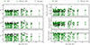 |
Fig. C.1. Electromagnetic properties of MBHBs and their host galaxies for MBHBs contributing 90% of the background. The left panels show B, V, and K magnitudes; the right panels radio flux at 2 GHz, X-ray flux at [2-10] keV and bolometric luminosity, where the horizontal line marks Lbol = 1045 erg s−1, as a typical value for quasar luminosities. Sources with magnitude fainter than 34 are set at 34, and similarly sources with X-ray flux < 10−19 and radio flux < 10−3 μJy are set at these values for clarity. For MBHs with fEdd < 10−3 we show an upper limit to the brightness ignoring the correction to radiative efficiency (filled squares) and a lower limit including the correction (empty squares connected to the filled squares). |
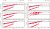 |
Fig. C.2. Ratio of AGN and galaxy luminosity for CW candidates. The left panels show the ratios in B, V, and K; the top and middle right panels the ratio in X-rays at [2-10] keV, and in radio at 2 GHz; the horizontal lines mark LAGN/Lgal = 1. The bottom-right panel shows the bolometric luminosity; the horizontal line marks Lbol = 1045 erg s−1. For MBHs with fEdd < 10−3 we show an upper limit to the brightness ignoring the correction to radiative efficiency (filled dots) and a lower limit including the correction (empty dots). |
All Tables
Configuration of the two toy PTAs used to infer the detectability of individual MBH binary.
All Figures
|
Fig. 1. Examples of the residence time (bottom panel), Δτc, per log10 orbital frequency bin are shown for three binaries from the HORIZON-AGN catalog, with chirp masses of 107, 108, and 109 M⊙. We also show their respective eccentricity evolution in the top panel. Eccentric systems are more efficient in dissipating the energy through GWs and this can be seen in the residence time (low panel) as compared to (nearly) circular binaries. The evolution of binaries at high frequencies (starting from a few nHz) is determined by the gravitational radiation, which is more efficient in energy dissipation for heavy and eccentric binaries. We also observe a fast circularization of eccentric systems in the top panel. |
| In the text | |
|
Fig. 2. 68% (dark) and 90% (light) confidence regions for the characteristic strain hc are shown for 2000 Universe realizations drawn from the HORIZON-AGN MBHB population, assuming either circular orbits (blue) or noncircular orbits (orange). We also plot their respective deterministic mean expectation values in dotted and dashed lines. For the circular population, we overlay as a dashed-dotted line the average spectrum, assuming the binary dynamics are driven by GW emission only. The inclusion of eccentricity introduces a significant signal reduction at frequencies lower than 10 nHz, due to the reduction of the MBHBs residence time at low orbital frequency. |
| In the text | |
|
Fig. 3. Median and 68% confidence interval of the differential contribution to the total characteristic strain signal, based on 2000 Universe realizations, shown across MBHB redshift bins for both circular and eccentric populations. We compare the results at two observer frequencies: 3.1 nHz (left panel) and 27.6 nHz (right panel). The vertical lines represent the median redshift values at which the cumulative contribution (integrating from low and high redshifts, respectively) reaches 5% of the total strain signal for the circular (solid line) and eccentric (dashed line) populations. |
| In the text | |
|
Fig. 4. Median and 68% confidence interval of the differential contribution to the total characteristic strain signal, based on 2000 Universe realizations, shown across MBHB log10-chirp mass bins for both circular and eccentric populations. We compare the results at two observer frequencies: 3.1 nHz (left panel) and 27.6 nHz (right panel). Vertical lines represent the median chirp mass value at which the cumulative contribution (integrating from lower masses) reaches 10% of the total strain signal for the circular (solid line) and eccentric (dashed line) populations. |
| In the text | |
|
Fig. 5. Comparison of the effective number of binaries in terms of N75 and Neff contributing to the GWB at each observed frequency bin of a PTA with an observing duration of 10.3 years as for EPTA Collaboration (2023a). At each observer frequency, the two extreme horizontal lines represent the 5th and 95th quartiles of the N75 distribution, derived from 2000 Universe realizations. The edges and the central line of the box represent the 25th, 50th, and 75th quartiles, respectively. For Neff, we only show the median of the distribution at each observer frequency with blue dots for the circular population and orange crosses for the eccentric population. |
| In the text | |
|
Fig. 6. Distributions of the amplitude Ayr at fyr and the spectral index γ, which parameterize the GWB timing residuals PSD, derived from 2000 Universe realizations, are compared with the EPTA results (red dotted contours) of EPTA Collaboration (2023a). The 68% and 90% confidence regions are shown for all distributions. Left panel: Distributions obtained via power-law least-squares fits to spectra from the Gaussian ensemble (GE) method for the circular (blue) and eccentric (orange) populations are shown as filled contours. Right panel: Distributions of maximum-a-posteriori power-law parameters from PTA-like inference using the GWB timing residuals from the population (Pop) approach. Solid contours represent the standard data analysis procedure that includes TMM; dashed contours represent the analysis without TMM. The effects of spectral leakage on the inference are clearly visible without TMM and remain measurable even when TMM is included. In both panels, the expected spectral index, γ = 13/3, of the average spectrum from a population of circular binaries driven by GW emission, is shown as a black vertical line. Note: γ relates to the characteristic strain spectral index α via γ = 3 − 2α. |
| In the text | |
|
Fig. 7. Comparison of the GW residuals RMS induced by the HORIZON-AGN population, using different modeling and populations, with the spectrum measured by the EPTA collaboration, shown in red. The average GE spectra of both circular and eccentric ensembles are depicted as solid and dashed lines, respectively. The distribution of the maximum-a-posteriori samples for the GWB spectra of the 2000 Universe realizations obtained using the population (Pop) method and a realistic PTA-like inference with and without TMM, are shown in dashed contours and light blue color, respectively, for the circular population. The effect of spectral leakage on the GWB inference results in a shallower spectral shape, significantly biasing the inference when TMM is not included. For some Universe realizations, spectral leakage still has appreciable effects at high frequencies even when TMM is applied. |
| In the text | |
|
Fig. 8. Probability of detecting a Continuous Wave (CW) signal from an individual MBH binary with a GW frequency in a given range, with an S/N greater than 3 for two toy PTAs representing the EPTA and the future SKA. Probabilities, shown as histograms, are derived from 2000 Universe realizations. The medians of the S/N distributions in each GW frequency band are overlaid, shown with dots (EPTA) and crosses (SKA). The frequency associated with the observation duration of the PTAs (10.33 years) is shown as a black vertical line. |
| In the text | |
|
Fig. 9. Properties of MBH binaries and their host galaxies, for systems dominating the background and CW candidates. From top to bottom, we show distributions of chirp mass, redshift and stellar mass of the host galaxy. The teal dotted histogram shows the distribution in the box volume (140 cMpc)3, the green histogram shows the simulation lightcone that models the galaxy distribution as seen by an observer, while the red hatched histogram shows CW candidates (‘CW cand’), with the gray histogram highlighting the high probability ones. In these distributions, we include CW candidates accounting for their multiplicity across Universe realizations. |
| In the text | |
|
Fig. 10. Environmental properties of MBH binaries and their host galaxies, for systems dominating the background (bck) and CW candidates (CW cand). From top to bottom, we show the chirp mass as a function of the stellar mass of the host galaxy and of the mass of the halo hosting the galaxy. Binaries hosted in central halos are shown as red squares; binaries hosted in subhalos are shown as orange crosses. An inner black marking highlights the high probability CW candidates. |
| In the text | |
|
Fig. 11. Properties of MBH binaries and their host galaxies, for systems dominating the background and CW candidates. Top: Eddington ratio of the binary averaged over 1 Myr around the time when the MBHs merge. Bottom: SFR averaged over 100 Myr. The teal dotted histogram shows the MBHBs dominating the background, selected in the simulation box. The red-hatched histogram shows CW candidates, with the gray histogram highlighting the high probability ones. MBHs with fEdd = 0 are shown at fEdd = 10−8 and galaxies with SFR = 100 Myr = 0 are shown at SFR = 100 Myr = 10−3. In these distributions we include CW candidates accounting for their multiplicity across Universe realizations. |
| In the text | |
|
Fig. 12. Left: Environment of a CW candidate binary with log10(ℳc/M⊙) = 9.02 and total mass log10(MBH/M⊙) = 9.97 at z = 0.025, hosted in a galaxy with log10(M★/M⊙) = 12.19 in a halo of mass log10(Mhalo/M⊙) = 13.44. Right: Environment of a CW candidate binary with log10(ℳc/M⊙) = 9.55 and total mass log10(MBH/M⊙) = 10.04 at z = 0.026, hosted in a galaxy with log10(M★/M⊙) = 12.69 in a halo of mass log10(Mhalo/M⊙) = 14.70. |
| In the text | |
|
Fig. 13. Left: Environment of a CW candidate binary with log10(ℳc/M⊙) = 9.07 and total mass log10(MBH/M⊙) = 10.16 at z = 0.032, hosted in a galaxy with log10(M★/M⊙) = 12.48 in a halo of mass log10(Mhalo/M⊙) = 14.44. Right: Environment of a CW candidate binary with log10(ℳc/M⊙) = 9.57 and total mass log10(MBH/M⊙) = 10.06 at z = 0.42, hosted in a galaxy with log10(M★/M⊙) = 12.40 in a halo of mass log10(Mhalo/M⊙) = 14.30. This is one of the highest redshift CW candidates in our analysis, and it is the progenitor of the MBH shown at later redshift in the left panel. |
| In the text | |
|
Fig. 14. Electromagnetic properties of MBHBs and their host galaxies for CW candidates. The left panels show B, V, and K magnitudes; the right panels show X-ray flux at [2–10] keV, radio flux at 2 GHz and bolometric luminosity (the horizontal line marks Lbol = 1045 erg s−1), as a typical value for quasar luminosities. For MBHs with fEdd < 10−3 we show an optimistic upper limit to the brightness ignoring the correction to radiative efficiency. |
| In the text | |
|
Fig. C.1. Electromagnetic properties of MBHBs and their host galaxies for MBHBs contributing 90% of the background. The left panels show B, V, and K magnitudes; the right panels radio flux at 2 GHz, X-ray flux at [2-10] keV and bolometric luminosity, where the horizontal line marks Lbol = 1045 erg s−1, as a typical value for quasar luminosities. Sources with magnitude fainter than 34 are set at 34, and similarly sources with X-ray flux < 10−19 and radio flux < 10−3 μJy are set at these values for clarity. For MBHs with fEdd < 10−3 we show an upper limit to the brightness ignoring the correction to radiative efficiency (filled squares) and a lower limit including the correction (empty squares connected to the filled squares). |
| In the text | |
|
Fig. C.2. Ratio of AGN and galaxy luminosity for CW candidates. The left panels show the ratios in B, V, and K; the top and middle right panels the ratio in X-rays at [2-10] keV, and in radio at 2 GHz; the horizontal lines mark LAGN/Lgal = 1. The bottom-right panel shows the bolometric luminosity; the horizontal line marks Lbol = 1045 erg s−1. For MBHs with fEdd < 10−3 we show an upper limit to the brightness ignoring the correction to radiative efficiency (filled dots) and a lower limit including the correction (empty dots). |
| In the text | |
Current usage metrics show cumulative count of Article Views (full-text article views including HTML views, PDF and ePub downloads, according to the available data) and Abstracts Views on Vision4Press platform.
Data correspond to usage on the plateform after 2015. The current usage metrics is available 48-96 hours after online publication and is updated daily on week days.
Initial download of the metrics may take a while.