| Issue |
A&A
Volume 705, January 2026
|
|
|---|---|---|
| Article Number | A52 | |
| Number of page(s) | 28 | |
| Section | Extragalactic astronomy | |
| DOI | https://doi.org/10.1051/0004-6361/202555588 | |
| Published online | 06 January 2026 | |
SN 2023gpw: Exploring the diversity and power sources of hydrogen-rich superluminous supernovae
1
Finnish Centre for Astronomy with ESO (FINCA), FI-20014 University of Turku, Finland
2
Department of Physics and Astronomy, FI-20014 University of Turku, Finland
3
Aalto University Metsähovi Radio Observatory, Metsähovintie 114, 02540 Kylmälä, Finland
4
Aalto University Department of Electronics and Nanoengineering, PO Box 15500 00076 Aalto, Finland
5
The Caltech Optical Observatories, California Institute of Technology, Pasadena, CA 91125, USA
6
Department of Physics and Astronomy, Aarhus University, Ny Munkegade 120, 8000 Aarhus C, Denmark
7
Center for Interdisciplinary Exploration and Research in Astrophysics (CIERA), Northwestern University, 1800 Sherman Ave, Evanston, IL 60201, USA
8
Cahill Center for Astrophysics, California Institute of Technology, MC 249-17, 1200 East California Boulevard, Pasadena, CA 91125, USA
9
INAF – Osservatorio Astronomico di Padova, Vicolo dell’Osservatorio 5, I-35122 Padova, Italy
10
Institute of Space Sciences (ICE, CSIC), Campus UAB, Carrer de Can Magrans s/n, 08193 Barcelona, Spain
11
Division of Physics, Mathematics, and Astronomy, California Institute of Technology, Pasadena, CA 91125, USA
12
Astrophysics Research Institute, Liverpool John Moores University, Liverpool Science Park, 146 Brownlow Hill, Liverpool L3 5RF, UK
13
Department of Astronomy, The Oskar Klein Centre, Stockholm University, AlbaNova, SE-106 91 Stockholm, Sweden
14
School of Physics, Trinity College Dublin, The University of Dublin, Dublin 2, Ireland
15
Instituto de Ciencias Exactas y Naturales (ICEN), Universidad Arturo Prat, Santiago, Chile
16
Institut d’Estudis Espacials de Catalunya (IEEC), Edifici RDIT, Campus UPC, 08860 Castelldefels (Barcelona), Spain
17
IPAC, California Institute of Technology, 1200 E. California Blvd, Pasadena, CA 91125, USA
★ Corresponding author: This email address is being protected from spambots. You need JavaScript enabled to view it.
Received:
20
May
2025
Accepted:
14
September
2025
Abstract
We present our observations and analysis of SN 2023gpw, a hydrogen-rich superluminous supernova (SLSN II) with broad emission lines in its post-peak spectra. Unlike previously observed SLSNe II, its light curve suggests an abrupt drop during a solar conjunction between ∼80 and ∼180 d after the light curve peak, which is possibly analogous to a normal hydrogen-rich supernova (SN). Spectra taken at and before the peak show hydrogen and helium “flash” emission lines attributed to early interaction with a dense confined circumstellar medium (CSM). A well-observed ultraviolet excess appears as these lines disappear, also as a result of CSM interaction. The blackbody photosphere expands roughly at the same velocity throughout the observations, indicating little or no bulk deceleration. This velocity is much higher than what is seen in spectral lines, suggesting asymmetry in the ejecta. The high total radiated energy (≳9 × 1050 erg) and aforementioned lack of bulk deceleration in SN 2023gpw are difficult to reconcile with a neutrino-driven SN simply combined with efficient conversion from kinetic energy to emission through interaction. This suggests an additional energy source, such as a central engine. While magnetar-powered models qualitatively similar to SN 2023gpw exist, more modeling work is required to determine if they can reproduce the observed properties in combination with early interaction. The required energy might alternatively be provided by accretion onto a black hole created in the collapse of a massive progenitor star.
Key words: stars: magnetars / stars: mass-loss / supernovae: individual: SN 2023gpw
© The Authors 2026
 Open Access article, published by EDP Sciences, under the terms of the Creative Commons Attribution License (https://creativecommons.org/licenses/by/4.0), which permits unrestricted use, distribution, and reproduction in any medium, provided the original work is properly cited.
This article is published in open access under the Subscribe to Open model. This email address is being protected from spambots. You need JavaScript enabled to view it. to support open access publication.
1. Introduction
Massive stars (≳8 M⊙) end their lives in luminous explosions known as supernovae (SNe). These explosions are divided into two main classes: hydrogen-poor SNe I and hydrogen-rich SNe II. For both types, there is also an analogous type of superluminous supernovae (SLSNe; for reviews see Gal-Yam 2012, 2019; Moriya 2026), which reach peak absolute magnitudes of ≲ − 20 mag and are thus a few or even several magnitudes more luminous than their normal counterparts. However, we note that for H-rich SLSNe, this limit is somewhat arbitrary, and some overlap is expected. Occasionally the peak magnitude can even approach ∼ − 23 mag (e.g. Kangas et al. 2022). Such luminosities, often paired with a relatively slow evolution, result in enormous energy requirements that the normal SN powering mechanisms – the decay of 56Ni and the cooling of the shock-heated envelope – cannot attain. Other power sources are therefore needed.
Such an SN could in principle be a so-called pair-instability SN (PISN; Barkat et al. 1967; Heger & Woosley 2002), where extreme temperatures resulting in pair production are reached at the core, decreasing radiation pressure and inducing a collapse. A PISN could power the luminosity with an extreme 56Ni mass, but there are only a few candidates for this mechanism (see, e.g., Lunnan et al. 2016; Schulze et al. 2024), and even then PISN models do not reproduce all main observables. In most cases, one of two main power sources is considered: either the birth of a strongly magnetized, fast-rotating neutron star, a millisecond magnetar, which subsequently acts as a central engine by shedding its rotational energy through magnetic braking (Kasen & Bildsten 2010; Woosley 2010), or the interaction between the ejecta and a dense circumstellar medium (CSM), resulting in efficient conversion of the kinetic energy of the ejecta into radiation (e.g. Chevalier & Fransson 1994; Ofek et al. 2007; Sorokina et al. 2016). Such interaction is common even among normal SNe II, where the ejecta may interact with as much as ∼0.5 M⊙ of CSM at early times (Morozova et al. 2018). In addition to the magnetar spin-down, another possible central engine is fallback accretion onto a nascent black hole (Dexter & Kasen 2013).
In SLSNe I, that is the more extensively studied SLSN type (e.g. Quimby et al. 2011; Chen et al. 2023a), the dominant mechanism is generally considered to be the magnetar central engine (e.g. Inserra et al. 2013; Nicholl et al. 2015; Gomez et al. 2024), though circumstellar interaction (CSI) seems to be required to explain some objects (e.g. Lunnan et al. 2018; Chen et al. 2023b). In particular, undulations commonly seen in SLSN I light curves (e.g. Inserra et al. 2017; Hosseinzadeh et al. 2022; West et al. 2023) may require CSI, though variations in the output of the central engine are plausible in some cases as well (Chugai & Utrobin 2022; Moriya et al. 2022; Chen et al. 2023b).
More luminous analogs to SNe IIn (i.e., with narrow Balmer lines indicative of CSI) form the majority of hydrogen-rich SLSNe (Gal-Yam 2019; Kangas et al. 2022; Pessi et al. 2025). As shown by Hiramatsu et al. (2024), the distribution of SNe IIn and their superluminous equivalents has no clear boundary. However, some SLSNe exhibit broad Balmer lines instead; the prototype of this subtype is SN 2008es (Gezari et al. 2009; Miller et al. 2009). In these objects, the lack of narrow lines from dense slow-moving CSM makes the dominant power source somewhat ambiguous, and both magnetars and CSI have been suggested (Inserra et al. 2018; Bhirombhakdi et al. 2019). In this paper, we follow the nomenclature of Gal-Yam (2019) and Kangas et al. (2022): We refer to the broad-lined subtype as SLSNe II and the narrow-lined one as SLSNe IIn for brevity.
In the largest sample of SLSNe II (i.e., not IIn) so far, Kangas et al. (2022) found sub-groups that spectroscopically resemble either SN 2008es or normal SNe II. The former group tends to be more luminous at its peak. While signs of CSI, such as an excess of ultraviolet (UV) emission over a blackbody, were seen, the magnetar and CSI models tended to be equally effective at reproducing the light curves. The most luminous SLSN II was estimated to emit ≳3 × 1051 erg. This poses a problem for the normal neutrino-driven core-collapse mechanism with CSI, as even with full conversion of kinetic energy into radiation, it seems impossible to obtain such an energy (Janka 2012), and it is possible that some SLSNe II require both a central engine and CSI. Whichever mechanism is dominant among SLSNe, they tend to occur in faint low-metallicity host galaxies, and SLSNe I and 2008es-like SNe seem to require an even lower metallicity than other SLSNe II or SLSNe IIn (e.g. Angus et al. 2016; Perley et al. 2016; Schulze et al. 2021; Kangas et al. 2022).
In this paper, we present UV, optical, and infrared photometric and spectroscopic observations of a SLSN II, SN 2023gpw. This SN exhibits a clear UV excess and early “flash” emission features similar to those seen early on in normal SNe II, which indicate CSI (e.g. Bruch et al. 2021; Jacobson-Galán et al. 2024). We analyzed the light curve and spectral evolution of the SN, comparing them to other SLSNe II in order to assess the physical nature of the transient. We present the data we used, both proprietary and public, in Sect. 2; our analysis is shown in Sect. 3; models of the photometric data of the SN and its host galaxy are in Sect. 4; and a discussion of our results is in Sect. 5. Finally, our conclusions are presented in Sect. 6. Throughout this paper, magnitudes are in the AB system (Oke & Gunn 1983) unless otherwise noted, and we assumed a ΛCDM cosmology with parameters H0 = 69.6 km s−1 Mpc−1, ΩM = 0.286, and ΩΛ = 0.714 (Bennett et al. 2014). Reported uncertainties correspond to 68% (1σ), and upper limits correspond to 3σ.
2. Observations
The discovery of SN 2023gpw in the Zwicky Transient Facility (ZTF; Bellm et al. 2019; Graham et al. 2019) on MJD = 60051.3 was reported by Förster et al. (2023). It was found at RA = 13:02:18.70, Dec = −05:51:10.95 using the Automatic Learning for the Rapid Classification of Events (ALeRCE) broker (Förster et al. 2021)1 and given the internal designation ZTF23aagklwb. We show the vicinity and faint host galaxy of the SN in Fig. 1. The photometric properties and the projected location near the nucleus of its host galaxy made the transient a candidate for a tidal disruption event (TDE) and prompted a spectroscopic observation as part of a TDE-related program (proposal P67-021, PI Charalampopoulos). The spectrum was taken on MJD = 60071.1 using the Alhambra Faint Object Spectrograph and Camera (ALFOSC) on the 2.56-m Nordic Optical Telescope (NOT) located at the Roque de los Muchachos Observatory, La Palma. The spectrum initially showed similarity to either a TDE or a SLSN II; the public classification of the event as a SLSN II and the SN 2023gpw designation (Kravtsov et al. 2023) was done later, on MJD = 60101.2, as part of the Public ESO Spectroscopic Survey for Transient Objects (PESSTO; Smartt et al. 2015)2. Based on the initial spectrum, we triggered a multi-wavelength follow-up as described below. The reduction of the resulting data is described in Appendix A.
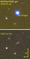 |
Fig. 1. Three-color NOT/ALFOSC images (blue: g; green: r; red: i) of SN 2023gpw a week before the light curve peak (left) and its faint host galaxy, visible at 189 d after the peak and with little contribution from the SN (right). The position of the SN in the galaxy is indicated, and the vertical bar corresponds to 10 arcseconds. |
Near-ultraviolet (NUV) observations of SN 2023gpw were performed with the Neil Gehrels Swift Observatory in the W1, M2, and W2 filters between MJD = 60075.8 and MJD = 60141.3. A late-time NUV template set containing only the host galaxy was also obtained on MJD = 60681.2. The data were downloaded using the HEASARC Archive3. Optical imaging of SN 2023gpw was done as part of ZTF using the ZTF Camera (Dekany et al. 2020) on the 48-inch Samuel Oschin Telescope at Palomar; the Spectral Energy Distribution Machine (SEDM; Blagorodnova et al. 2018) on the Palomar 60 inch (P60) telescope in the gri bands; and the IO:O instrument on the 2-m robotic Liverpool Telescope (LT; Steele et al. 2004) located at La Palma, in the griz bands. Outside ZTF, we used the Las Cumbres Observatory Global Telescope (LCOGT; Brown et al. 2013) network (proposal OPTICON 22A/012, PI Stritzinger) in the ugri bands. We also obtained one epoch of ugri photometry and four epochs of late-time (after MJD = 60289) gri photometry using NOT/ALFOSC as part of the NOT Un-biased Transient Survey 2 (NUTS2) collaboration4 (proposal 66-506, PIs Kankare, Stritzinger, Lundqvist). In the near-infrared (NIR), we obtained one epoch in the JHKs bands using the Nordic Optical Telescope near-infrared Camera and spectrograph (NOTCam) on the NOT as part of NUTS2. All our photometric measurements, without K-corrections or extinction corrections, are shown in Appendix B in Tables B.1 to B.7. Finally, we acquired one epoch (MJD 60081.01) of V and R-band imaging polarimetry with NOT/ALFOSC. All observations were obtained at four half-wave plate angles (0°, 22.5°, 45°, 67.5°) with an exposure time of 100 seconds per half-wave plate.
Spectroscopic observations of SN 2023gpw were performed using the following instruments:
-
Three spectra using NOT/ALFOSC: One on MJD = 60071.1 and two as part of NUTS2 on MJD = 60077.0 and 60084.9;
-
Two spectra using the Intermediate Dispersion Spectrograph (IDS) on the 2.5-m Isaac Newton Telescope (INT) at La Palma on MJD = 60097.0 and 60097.9 (proposal C54, PI Müller-Bravo);
-
Two spectra using the Double Beam Spectrograph (DBSP; Oke & Gunn 1982) on the Palomar 200-inch Telescope (P200) in Palomar, California, USA, as part of ZTF on MJD = 60116.2 and 60137.3;
-
Twelve spectra using SEDM as part of ZTF between MJD = 60071.2 and 60121.2;
-
A late-time spectrum using the Optical System for Imaging and low-Intermediate-Resolution Integrated Spectroscopy (OSIRIS+) instrument on the 10.4-m Gran Telescopio Canarias (GTC) at La Palma on MJD = 60386.2 (proposal GTCMULTIPLE2G-24A, PI Elias-Rosa).
The properties of these spectra are listed in Table B.8.
In addition to proprietary data, we retrieved the public PESSTO classification spectrum of SN 2023gpw (Kravtsov et al. 2023) from the Transient Name Server (TNS)5. This spectrum was taken on MJD = 60101.2 with the ESO Faint Object Spectrograph and Camera 2 (EFOSC2) instrument on the New Technology Telescope located in La Silla, Chile. We also obtained the Asteroid Terrestrial-impact Last Alert System (ATLAS; Tonry 2011; Smith et al. 2020) forced photometry (Shingles et al. 2021) of SN 2023gpw, which extends from MJD = 60100.8 to MJD = 60169.0 in the ATLAS wide-band c and o filters.
3. Analysis
3.1. Light curve
We applied a Milky Way extinction correction of AV, MW = 0.097 mag (Schlafly & Finkbeiner 2011) to our photometry, using the Gordon et al. (2023) extinction law (with RV = 3.1). The observed early blue color (see below and Sect. 4.1) and a lack of narrow interstellar absorption lines, especially from Na I (Sect. 3.2), suggest a minimal host-galaxy extinction, and we only correct our photometry for the Milky Way extinction in this paper. Our host-galaxy fitting (Sect. 4.3) agrees with this result.
Due to the heliocentric redshift z = 0.0827 ± 0.0002 of SN 2023gpw based on host-galaxy lines (see Sect. 3.2), we also apply an approximate K-correction (Hogg et al. 2002) of −2.5log(1 + z)≈ − 0.09 mag (i.e., we add 0.09 to the observed magnitude). This approximation was shown to work reasonably well for SLSNe II in the optical by Kangas et al. (2022). For SN 2023gpw, we used the SNAKE code (Inserra et al. 2018) to determine spectroscopic K-corrections in the g and r bands, which we use for light curve comparisons. These were found to be close to the above approximation (−0.08 mag in g and −0.12 mag in r) around the peak. In the NUV and NIR bands, we do not have spectra available, and in the NIR, only one epoch of photometry for determining the K-correction. Therefore, we only applied the approximate correction in all bands, which keeps the object comparable to the literature sample.
Based on the redshift – in the Galactic standard of rest, zGSR = 0.0824 ± 0.0002 – and the assumed cosmology, we obtained a luminosity distance of DL = 377.3 ± 1.0 Mpc and a distance modulus of μ = 37.88 ± 0.01 mag. The rest-frame absolute-magnitude light curve is shown in Fig. 2. For clarity, ATLAS magnitudes were averaged when multiple observations were performed within 0.1 d.
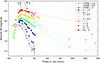 |
Fig. 2. Light curve of SN 2023gpw. The zero epoch corresponds to the g-band peak on MJD = 60085.0. Triangles denote 3σ upper limits, and shaded regions denote 1σ uncertainties of our GP fits. Epochs of spectra are marked with black (SEDM), gray (our other spectra) or blue (Kravtsov et al. 2023) lines, and the epoch of polarimetry is marked with a red line. Dashed lines show the evolution if the pre-gap decline rates had stayed constant during the gap, showing that the decline must have steepened some time after the last detection in the r and i bands. |
We performed numerical interpolation of the light curves using a Gaussian process (GP) regression algorithm (Rasmussen & Williams 2006) to estimate the peak magnitudes and epochs. We used the Python-based george package (Ambikasaran et al. 2015), which implements various kernel functions. The widely used Matérn-3/2 kernel was applied, with a 0.05 mag error floor added to measured magnitudes to avoid overfitting because of individual points, and hyperparameters were not fixed. The 1σ lower and upper bounds of the peak epoch were conservatively estimated as the epochs when the maximum-likelihood GP fit becomes, respectively, brighter and fainter than the 1σ lower bound on the peak brightness.
The peak epoch in the g-band is MJD , which we use as the reference epoch in the rest of the paper. The peak absolute magnitude in g is Mg, peak = −21.58 ± 0.03 mag, which makes SN 2023gpw relatively luminous among the SLSNe II of Kangas et al. (2022), roughly on the borderline between SLSNe II that spectroscopically resemble normal SNe II and those that resemble SN 2008es. The measured peak epochs and magnitudes in all bands are listed in Table 1. The light curve peaks slightly earlier and is brighter at shorter wavelengths. In the NUV bands, the peak epoch cannot be determined due to a lack of pre-peak observations; however, by eye (Fig. 2), the peak seems to be close to the first observed epoch (MJD = 60075.8) in all NUV bands and certainly earlier than in the optical.
Epochs and absolute magnitudes at peak in the optical bands.
The observed photometric evolution of SN 2023gpw is relatively smooth, with no clear bumps or other conspicuous features. Simply based on the first detection at MJD = 60051.3 and the g-band peak, the rise time is ≳31 d. The ZTF photometry does not include a constraining non-detection before the first detection (the last two r-band non-detections at MJD = 60049.3 and 60045.3 have upper limits of ≥20.4, brighter than the first detection with r = 20.78 ± 0.32 mag), but based on our GP fits, we can calculate the g-band rest-frame rise time from 10% of the peak brightness,  d; from 1/e of the peak brightness,
  d; and from half-maximum,
  d. This rise is relatively fast compared to the SLSNe II in Kangas et al. (2022), especially compared to other SLSNe II peaking at < − 21 mag, and to the SLSNe IIn in Pessi et al. (2025). The decline rate after the peak depends on wavelength, with bluer bands declining faster. Optical decline rates measured using a linear fit between +20 and +54 d are 0.061 ± 0.004 mag d−1 in u, 0.034 ± 0.001 mag d−1 in g, 0.017 ± 0.001 mag d−1 in r, and 0.012 ± 0.002 mag d−1 in i.
After ∼ + 55 d, SN 2023gpw entered solar conjunction and no observations were performed in most filters until +189 d. In the meantime, only ATLAS photometry exists, extending to +78 d in the c-band and +70 d in the o-band. After this gap, no source is detected after host-galaxy subtraction. It is clear, however, that at the rate the r- and i-band light curves were declining when the gap began, they would not have reached the post-gap limits; in particular, in the i band, there is a difference of almost 4 mag (see Fig. 2). Some time during this gap, a drop of multiple magnitudes (depending on the filter) occurred. The drop had not yet begun at +78 d, the epoch of the last ATLAS detection. No further ATLAS data exist until after the gap, where only shallow limits (not deep enough to reach the host magnitude) are available. No clear broad lines from the SN are seen in a GTC/OSIRIS+ spectrum of the host galaxy taken at the position of the SN at +278 d, corroborating this result (see Sect. 3.2). Instead of an abrupt drop followed by a slower decline in SN 2023gpw, however, we cannot fully exclude a more gradually steepening light curve more similar to, for example, SN 2021irp (Reynolds et al. 2025).
We show a comparison between the g- and r-band absolute light curves of SN 2023gpw and other SLSNe II in Fig. 3. We include the Kangas et al. (2022) sample, the prototypical SLSN II event SN 2008es (Gezari et al. 2009; Miller et al. 2009; Bhirombhakdi et al. 2019), CSS121015:004244+132827 (hereafter CSS121015; Benetti et al. 2014), and the objects in Inserra et al. (2018). For objects with z > 0.17, the observed r (i)-band was converted to the rest-frame g (r)-band. The g-band evolution of SN 2023gpw resembles that of SN 2008es and especially SN 2013hx, which exhibited a similar peak magnitude and decline, though SN 2023gpw rises to the peak faster than SN 2013hx and the rise of SN 2008es is not well constrained. Even at late times, these two SNe are within ∼0.5 mag of the limits we set for SN 2023gpw in the g-band (but a large gap in the light curve of SN 2013hx makes this less clear). By peak luminosity, SN 2023gpw is the sixth-brightest out of these 17 objects. The steepening light curve of SN 2023gpw during the solar conjunction is more pronounced in the r band; such a drop is not observed among other SLSNe II, but there are several objects where a drop around +100 d cannot be excluded due to a lack of data. Late-time observations of SN 2008es (Bhirombhakdi et al. 2019) show that its light curve did not experience a steepening; instead, it declined relatively steadily until almost +300 d.
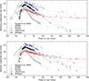 |
Fig. 3. Top panel: Absolute g-band light curve of SN 2023gpw (black) compared to other SLSNe II. We include the SLSNe II presented by Kangas et al. (2022) (gray), the prototypical SN 2008es (purple; Gezari et al. 2009; Miller et al. 2009), CSS121015 (Benetti et al. 2014), and the two SLSNe II presented by Inserra et al. (2018) (SN 2013hx in teal and PS15br in red). Bottom panel: Same but in the r-band. A pronounced steepening in the r-band light curve, such as that in SN 2023gpw at some point before ∼ + 200 d, is not observed in other SLSNe II, though it is not excluded in some objects whose light curves do not continue this long. In both panels, the zero epoch corresponds to the g-band peak. |
We show the color evolution of SN 2023gpw in Fig. 4, with the g − r color also compared to other SLSNe II (all corrected for Milky Way extinction). For the measured colors, we use data points within 0.1 d of each other in time. In the top panel, we also show the differences between the GP interpolations at each band as shaded regions, while in the bottom panel, the GP interpolations of comparison events are shown as lines. The uncertain early g − r color is consistent with practically no change, as is the r − i color. From around the peak, all measured colors (u − g, g − r, and r − i) become steadily redder over the rest of the light curve. The evolution of the u − g color is the fastest, increasing from ∼0 mag at peak to ∼1.3 mag at 55 d. The g − r color, between ∼ − 0.3 mag at −10 d and 0.5 mag at 50 d, is initially bluer than that of SN 2008es (Gezari et al. 2009) or most SLSNe II in the Kangas et al. (2022) sample, but also reddens faster than most SLSNe II and eventually reaches a similar color.
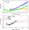 |
Fig. 4. Top panel: Optical colors of SN 2023gpw interpolated using a GP fit (shaded regions denote the 1σ uncertainty of this fit). The g − r color seems to become bluer during the rise to the peak, but the uncertainties of the measured colors are also consistent with no evolution in g − r until around the peak. Bottom panel: Comparison of the g − r color of SN 2023gpw with other SLSNe II (Miller et al. 2009; Inserra et al. 2018; Kangas et al. 2022), all corrected for Galactic extinction. The colors of comparison SNe have been GP-interpolated for visual clarity. |
We used SuperBol (Nicholl 2018) to construct a pseudo-bolometric light curve. The r-band was used as the baseline, and other optical and NUV light curves were interpolated to the r-band epochs using a polynomial fit within SuperBol. Extrapolation of the early light curve before the first NUV and i points was performed by assuming a constant color. Extrapolation to the end of the observations was done using c as the baseline and assuming constant colors in the bands not observed between +54 and +78 d. NIR data were only available at one epoch and were not included. Blackbody-based bolometric corrections are performed in SuperBol, but we do not include them, as NUV data of SN 2023gpw deviate from a blackbody at most epochs (see Sect. 4.1); this also means that our pseudo-bolometric luminosities are lower limits for the total bolometric luminosity. The pseudo-bolometric light curve is displayed in Fig. 5.
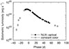 |
Fig. 5. SuperBol (Nicholl 2018) pseudo-bolometric light curve of SN 2023gpw. The values shown are based on either the full NUV-optical range (solid points) or only two or three bands and constant-color-based extrapolation of other bands (open points). |
The pseudo-bolometric luminosity at its peak, at ∼ − 5 d, is (2.8 ± 0.3)×1044 erg s−1. It then declines by about a factor of 20 by the time of the solar conjunction. Before the conjunction the decline slows down slightly, but no bump or plateau is observed and the decline is smooth. Integrating over this light curve, we estimated the energy radiated by SN 2023gpw in the observed filters to be (8.91 ± 0.21)×1050 erg, making this a lower limit for the total energy radiated across all wavelengths. Kangas et al. (2022) found similar or even greater energy requirements for the most luminous, 2008es-like SLSNe II.
3.2. Spectroscopy
The spectra of SN 2023gpw used in this paper, except the low-resolution SEDM spectra, are shown in Fig. 6, including the classification spectrum (Kravtsov et al. 2023); the SEDM spectral sequence is shown in Fig. 7. In the earliest spectra between −13 d and the peak, the visible features are Balmer lines and He IIλ4686, of which Hα and He II are also visible in the SEDM spectra. Such “flash” features are common among normal SNe II (Bruch et al. 2021, 2023). The Hβ and Hγ are faint in the ALFOSC spectrum at −13 d, but their presence is clear at −7 d and consistent with the −13 d spectrum. In Fig. 8, we show the Hα profile evolution in particular; at early epochs this is compared to He IIλ4686. The Hα profile consists of a central narrow or intermediate-width component surrounded by broad wings, likely caused by electron scattering; the wings are quite clear at −13 and −7 d, but at peak, they have weakened. The full width at half-maximum (FWHM) of the narrow component is ∼1000 km s−1 in the ALFOSC spectra from −13 d to the peak. The velocity resolution at this wavelength is 680 km s−1, implying a marginally resolved line with an intrinsic width of ∼700 km s−1. The Hβ line also exhibits a similar profile, but we see no clear narrow component in the He IIλ4686 line, which can be fit using either a Lorentzian or a Gaussian function (residuals in both cases are dominated by noise), with a FWHM between 6400 and 7300 km s−1 depending on the spectrum and the function. By eye, the He IIλ4686 line appears similar to the broad component of Hα at −13 d. At all these epochs, the peak of He IIλ4686 is blueshifted by between 1000 and 2000 km s−1, while the narrow component of Hα is at zero velocity.
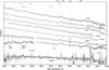 |
Fig. 6. Our moderate-resolution spectra of SN 2023gpw. Savitzky-Golay smoothing has been applied, and the +12-d spectrum has been binned by a factor of five. The original spectra are plotted in gray. The zero epoch corresponds to the g-band peak on MJD = 60085.0. Telluric absorption is marked with the ⨁ symbol and vertical dotted lines. The +278-day spectrum has no clear SN lines; only narrow emission lines from the host galaxy can be seen. Extinction correction has not been applied. The public PESSTO spectrum at +15 d does not include telluric-line correction. |
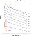 |
Fig. 7. Low-resolution SEDM spectra of SN 2023gpw. The zero epoch corresponds to the g-band peak on MJD = 60085.0. Telluric absorption lines (⨁) are marked in vertical dotted lines. The marked lines are based on the higher-resolution spectra; the Ca II lines do not seem to match observed features here. |
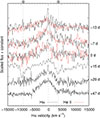 |
Fig. 8. Evolution of the Hα (black) and He IIλ4686 (red) line profiles in SN 2023gpw with the continuum subtracted on both sides. Telluric lines around Hα (⨁) are marked with dotted lines and the zero velocity with a dashed line. A weakening narrow component can be seen in the profile, while the wings of the broad component are disturbed by the telluric lines, but extend to several thousand km s−1 on both sides. |
All of these lines get weaker toward the peak, after which they disappear. Instead, we start to see a weak P Cygni profile of He Iλ5876 and a broad Hα line with a much weaker or non-existent narrow component. Neither kind of Hα line is visible in the SEDM or INT/IDS spectra at +12 d, but the broad profile appears in later spectra starting at +15 d. The He Iλ5876 line, on the other hand, is already visible at +12 d. The velocity of the He Iλ5876 absorption minimum in the better-quality spectra at +15 and +29 d is between 4000 and 4500 km s−1.
Telluric lines are strong in the PESSTO classification spectrum (Kravtsov et al. 2023) and make it difficult to measure the Hα velocity, but the profile in our DBSP spectra at +29 and +47 d can be fit using a Gaussian with a FWHM of ∼5500 km s−1. The profile at +29 and +47 d extends to roughly 5000 km s−1 on the blue side and slightly less on the red side, with the broad component blueshifted by ∼1000 km s−1, similarly to the early He II. The Hβ line is located close to the edge of the blue grating of DBSP and is difficult to fit. On top of the broad Hα, there is a weak unresolved (270 km s−1) component; this putative component is not much stronger than the noise level in the +47 d spectrum, but seems to be present at zero velocity at both epochs, similarly to the narrow component in the first two spectra. This weak narrow Hα line is likely at least partially from the host galaxy. In any case, after the peak, the Balmer lines are dominated by the broad component.
The +47 d spectrum also shows apparent broad absorption lines in its red part. Atmospheric features likely contribute to this, as the +47-d spectrum was taken at a relatively high airmass during early twilight due to SN 2023gpw setting very early that night. The Ca II NIR triplet is possibly present as well, but not clearly so. In the blue parts of the +29 and +47-d spectra, we see other broad lines appearing. These include the Mg I] λ4571 and Ca II doublets at λλ3706,3736 and λλ3934,3968. Unlike the Balmer lines, all of these seem to be redshifted by ∼2500 km s−1; it is also possible that these features have a contribution from nearby iron lines. The SEDM spectrum at +33 d does not seem to match the Ca II identification, but it is also very noisy; the Mg I] λ4571 line, on the other hand, is present. The He Iλ5876 line is no longer apparent at +47 d, but a broad feature possibly attributable to O Iλ6157 appears at +29 and +47 d.
We used the late-time GTC spectrum on MJD = 60386.2 (+278.4 d) to determine the redshift of SN 2023gpw. The spectrum is dominated by narrow host-galaxy emission, with no visible broad emission lines from the SN, except something that looks like an [O I] λλ6300, 6364 feature; this emission, however, is only visible in one of the two OSIRIS exposures, and the 6364 Å component is missing, making it a likely artifact. No broad Hα, ubiquitous in late-time spectra of SLSNe II (Kangas et al. 2022), is seen. We do, however, detect narrow lines of Hβ, [O III] λλ4959, 5007, and Hα, and using these lines we measured an average redshift of z = 0.0827 ± 0.0002. The strength of the [O III] λλ4959, 5007 doublet compared to Hα suggests that the latter is also dominated by host galaxy emission and has little contribution from the SN. The lack of broad lines at such a late phase indicates that the observed emission is generally dominated by the host galaxy, which is consistent with the late-time non-detections in our photometry (Sect. 3.1).
We show a comparison between SNe 2008es and 2023gpw in Fig. 9, and a comparison to those SLSNe II that Kangas et al. (2022) considered more spectroscopically reminiscent of normal SNe II in their sample in Fig. 10. Similarities can be seen to several objects; the strengths of the emission lines resemble those of SN 2008es, but the shape of the Hα line is more similar to the latter group, albeit narrower than most. The spectra of the SLSNe II resembling normal SNe II almost all reach later epochs than what we have access to with SN 2023gpw, so we cannot say for sure whether its Hα profile starts to resemble them later. The metal lines, if originating from Mg I] λ4571 and Ca II, would be similarly redshifted in the comparison objects, suggesting that there is, in fact, a large contribution from iron. In some cases, absorption components in P Cygni profiles are very clear, which we do not see in SN 2023gpw. Perhaps the best match to SN 2023gpw at +47 d among other SLSNe II is SN 2020bfe at +63 d; however, no spectra of this SN exist between −14 and +63 d (Kangas et al. 2022). The same problem applies to other similar SLSNe II. At −14 d, SN 2020bfe does show multi-component emission lines as well, but only those of hydrogen. Similarly to SN 2023gpw, SN 2020bfe also shows no Hα absorption component and a weak He Iλ5876 (+Na Iλλ5890, 5896) feature. However, SN 2020bfe was over a magnitude fainter at peak and did not exhibit a steepening light curve during a follow-up extending to ∼ + 220 d.
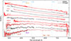 |
Fig. 9. Spectral evolution of SN 2023gpw (black) compared to the prototypical SN 2008es (red). Savitzky-Golay smoothing has been applied; the original spectra are plotted in gray. The zero epoch corresponds to the g-band peak. |
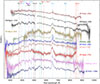 |
Fig. 10. Spectral evolution of SN 2023gpw (black) compared to SLSNe II that resemble normal SNe II more than they do SN 2008es (Kangas et al. 2022). Savitzky-Golay smoothing has been applied; the original spectra are plotted in gray. The zero epoch corresponds to the g-band peak. |
3.3. Polarization
The intensity-normalized Stokes parameters (q = Q/I and u = U/I, where Q and U are the differences in flux with the electric field oscillating in two perpendicular directions, and I is the total flux) were used to calculate the polarization degree ( ) and the polarization angle (χ = 0.5arctan(u/q)). All values of p presented in this paper have been corrected for polarization bias (e.g. Simmons & Stewart 1985; Wang et al. 1997) following Plaszczynski et al. (2014).
In the V-band, we measured q = (0.50 ± 0.24)% and u = (0.72 ± 0.25)%, while in the R-band we measured q = (0.41 ± 0.26)% and u = (0.34 ± 0.26)%. This led to p = (0.84 ± 0.25)% and χ = (27.61 ± 8.07)° in the V-band, and p = (0.47 ± 0.26)% and χ = (19.83 ± 13.98)° in the R-band. The two bands are mutually consistent within 1σ in both polarization degree and angle, with an average degree of p = (0.66 ± 0.26)%. As the spectrum of the target is, at this epoch (−3.7 d), continuum-dominated, real differences between the bands from depolarization caused by lines are disfavored.
In order to properly isolate the intrinsic polarization, the effect of the interstellar polarization (ISP), introduced by dust grains in the line of sight, has to be estimated. Unfortunately, there are no stars with adequate S/N in the field of view of our ALFOSC observations. Another way to roughly estimate the Galactic ISP is as 9 × E(B − V) % (Serkowski et al. 1975), and for SN 2023gpw, this would be ∼0.27 %. We also checked for polarization standard stars published in Heiles (2000) that are close to the location of SN 2023gpw. We find one star within two degrees from SN 2023gpw (∼1.24°) with a polarization value of pISP = (0.26 ± 0.07)%, consistent with the above estimate. Based on the host galaxy (see Sect. 4.3), there is no evidence for strong reddening, and hence we neglect the ISP of the host. In Fig. 11 are shown the Stokes q – u planes for the imaging polarimetry, and the ISP estimate as a gray filled circle. The ISP, with a degree of pISP = 0.27 % and an unknown angle, cannot be directly removed from the observed polarization, but rather introduces an additional uncertainty of  %, for a total of p = (0.66 ± 0.33)%, only 2σ above zero polarization.
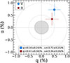 |
Fig. 11. Intensity-normalized Stokes q and u parameters of our polarimetry in the V and R bands on MJD = 60081.0, corresponding to −3.7 d. The filled circle corresponds to our best ISP estimate (see text) and the dashed circles to 0.5% and 1.0% polarization. The two bands are consistent with each other within 1σ and higher than the ISP. |
Another thing to consider, when dealing with nuclear transients, is the effect of dilution by unpolarized light from the host galaxy. However, in the case of SN 2023gpw, the host is much fainter than the transient during our epoch of observation (see Sect. 4.3), and hence the effect is negligible. Considering all of the above, we conclude that SN 2023gpw is likely intrinsically polarized, though its low significance makes it impossible to be certain. This polarization would indicate asphericity in SN 2023gpw during the epochs before and/or around the peak.
4. Modeling
4.1. Blackbody fits
We performed blackbody fits to the spectral energy distributions (SEDs) of SN 2023gpw using our NUV, optical, and NIR photometry. This was done at each NUV epoch; in the optical, we used our GP-interpolated light curves (see Sect. 3.1) to match these epochs. The NIR data points cannot be interpolated as we only have one epoch, but on MJD = 60109.9 they are close to the NUV epoch on MJD = 60108.6 and were used in the fit at this epoch. Starting at +18 d, an excess over the blackbody function is immediately apparent in the NUV, and the W2 and M2 bands were ignored in the fits at +18 d and afterward. These fits are shown in Fig. 12. Earlier, the NUV points match well with the blackbody (though the u-band point at −8 d may deviate from the other points). The flattening NUV spectrum does not strongly affect the W1 band, which is compatible with the same blackbody as the optical and NIR data. Before the start of our NUV follow-up, we only have the ZTF gri-band data available, and the resulting blackbody fits are less robust.
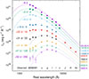 |
Fig. 12. Blackbody fits (lines) to the observed SEDs of SN 2023gpw (points). An excess over the blackbody function appears and gradually strengthens after the peak. The W2 and M2 bands have been ignored in the fits denoted with dashed lines; the W1-band is roughly compatible with the optical data throughout the evolution. |
We show our blackbody parameters, the temperature and the radius, in Fig. 13, including the fits based only on the gr(i) bands. The blackbody radius increases linearly over time; a fit to this expansion (ignoring the epochs before NUV observations) results in a photospheric velocity of vph = 9080 ± 430 km s−1, significantly higher than the spectroscopic velocities measured from the hydrogen and helium lines. Extrapolating the best-fit velocity to earlier epochs, we obtain an explosion date of −28.9 ± 1.6 d, which is close to the discovery epoch at −31.1 d and hints that the SN was indeed discovered quite close to the explosion (or, in principle, that the expansion speed increased early on). The temperature at early times is not particularly reliable as we only have two or three bands available, but it seems to increase during the rise based on the g − r color. At peak, the temperature is ∼20 000 K (similar to the hottest SNe II at peak, but somewhat later due to the slower rise; see Faran et al. 2018). This then declines to ∼10 000 K by ∼+20 d and, afterward, declines more slowly to around 6000 K at +50 d.
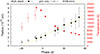 |
Fig. 13. Evolution of the blackbody temperature (red) and radius (black) of SN 2023gpw. The empty symbols are based on less reliable fits using only the gr(i)-band data. The yellow line corresponds to the best-fit expansion velocity using the solid points only; this line reaches zero radius at −29 d, which is close to the first observed epoch at −31 d. |
4.2. Light curve fits
We used the publicly available code Modular Open Source Fitter for Transients (MOSFiT6; Guillochon et al. 2018) to fit the multi-band light curve. We included the radioactive 56Ni decay model (Arnett 1982; Nadyozhin 1994), labeled default; a CSI model (Chatzopoulos et al. 2013; Villar et al. 2017; Jiang et al. 2020), labeled csm; a fallback accretion model (Moriya et al. 2018), labeled fallback; and a magnetar central engine model (Kasen & Bildsten 2010), labeled magnetar, included in the code. The W2 and M2 light curve data were ignored in our fits, as a UV excess is not reproduced in these models. The slsn model (Nicholl et al. 2017) is a modified version of the magnetar model with constraints for more plausible physical parameters, limiting the neutrino energy to ∼1051 erg and cutting out models that become nebular before 100 d. However, it also includes a modified blackbody with absorption below 3000 Å. This is commonly observed in SLSNe I but not in SN 2023gpw, where we would also need to ignore the W1 band. Hence, we instead modified the magnetar model file to include the same constraints.
These models were fitted using the dynamic nested sampling package dynesty (Speagle 2020)7. We ran each fitting process until convergence, which typically took between 15 000 and 25 000 iterations. The quality of the fit is quantified by a likelihood score returned by MOSFiT, corresponding to the logarithm of the Bayesian evidence Z.
We set simple, broad, and uniform or log-uniform priors for each free parameter (summarized in Table 2 for each model). Based on the lack of narrow Na I D absorption lines in the spectra, we set an upper limit for the host galaxy extinction, AV, host ≤ 1 mag. Host extinction itself is not a parameter in MOSFiT; however, a related quantity, the column density of neutral hydrogen, nH, host, is. We therefore set the upper limit as nH, host ≤ 2 × 1021 cm−2 based on Güver & Özel (2009), similar to Kangas et al. (2022).
Free and fixed parameters used in each MOSFiT model fit to the second peak, with prior distributions indicated.
Other parameters common to all models include the time from explosion to observations texpl, the minimum temperature Tmin, and the ejecta mass Mej. We fixed the (Thomson scattering) opacity κ at 0.34 cm2 g−1, a typical value for hydrogen-rich ejecta and close to the result of Nagy (2018). This parameter is included in all models used here except the CSI model.
The 56Ni model also includes the nickel fraction in the ejecta fNi and the opacity to γ-rays κγ. The magnetar model includes the spin period Pspin, the magnetic field perpendicular to the spin axis B⊥, the neutron star mass MNS, and the angle between the magnetic field and spin axis θPB. In the CSI model, we assumed a hydrogen-rich progenitor, but not necessarily an extended envelope. Thus the minimum inner radius of the CSM, R0, was set at 0.1 AU (∼20 R⊙), roughly half the radius of the blue supergiant progenitor of SN 1987A (Podsiadlowski 1992), but larger than a Wolf-Rayet progenitor of a stripped-envelope SN. From the disappearance of the “flash” emission lines before +12 d, ≳43 d after the explosion, and the ejecta velocity of 9100 km s−1, we can estimate that some part of the CSM has been encountered by the ejecta before 3.4 × 1015 cm, corresponding to ≲230 AU; conservatively, we set the upper limit for R0 at 250 AU. The density of the CSM at R0, ρ, is also a free parameter. We fixed the density power-law parameters in the inner (ρej ∝ r−δ) and outer (ρej ∝ r−n) ejecta, δ = 1 and n = 12, respectively – normal values in hydrogen-rich ejecta (Chatzopoulos et al. 2013). The density power law of the CSM (ρCSM ∝ r−s) was fixed at either s = 0 or s = 2, respectively corresponding to a constant-density or wind-like CSM. Finally, the fallback model includes the linear-to-power-law accretion transition time ttr and the accretion luminosity at the transition time L1.
In total, the default and fallback models have eight free parameters, the csm model has nine, and the magnetar model has ten. This includes a nuisance parameter σ, which describes the added variance required to match the model being fitted. The outputs of the MOSFiT modeling are shown in Fig. 14. The median posterior values of each free physical parameter, with the 16th and 84th percentile values as uncertainties, along with the Bayesian evidence score of each model, are listed in Table 3. The corner plots of the fits, which also include σ, can be found in the appendices in Figs. C.1 to C.5.
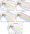 |
Fig. 14. MOSFiT light curve fits to SN 2023gpw using the different models described in the text. Late-time upper limits are represented as points, and the 3σ uncertainty corresponds to the measured limit. All models, but especially magnetar and fallback, have trouble reproducing the drop in brightness during the gap. The best fit by eye and score is the CSM model with s = 0. |
Median posterior values and uncertainties of free parameters in each MOSFiT model fit and the score of each model.
It is clear that, with these constraints, the default model cannot account for the rise and decline times of the light curve simultaneously with its luminosity. This is unsurprising, as the 56Ni decay model is incompatible with SLSNe II in general (Kangas et al. 2022). The magnetar and fallback models can somewhat replicate the early light curve, but both models result in a power-law decline at late times (t−2 or t−5/3, respectively), which over-predicts the flux after the solar conjunction. In the csm model with s = 2, the late-time behavior is still off, though to a somewhat lesser degree. Meanwhile, the s = 0 case looks quite different and does produce a sufficient drop in brightness during the gap. It is also the best fit by MOSFiT score, albeit very narrowly. In the s = 2 model, the (hydrogen-rich) SN ejecta, with a large mass of  M⊙, would interact with a CSM of
  M⊙, while in the s = 0 case, we obtain a smaller ejecta mass of 6.8 ± 1.0 M⊙ with a larger CSM mass, 4.0 ± 0.2 M⊙. All these models except default return explosion times between ∼1 and ∼3 days before the first detection of SN 2023gpw, indicating that it was caught soon after the explosion.
4.3. Host galaxy
To quantify the proximity of the transient to the nucleus of the host galaxy, we first aligned our late-time r-band images, dominated by the host galaxy, at sub-pixel precision using the Image Reduction and Analysis Facility (IRAF8) tasks geomap and geotran, then added these together to create a stacked host galaxy image. We then performed a Markov Chain Monte Carlo fit of a two-dimensional Sérsic profile to this image using the Sersic2D function in astropy9 and the emcee10 package (Foreman-Mackey et al. 2013) to find the centroid in pixel space (with the centroid, Sérsic index, ellipticity, and position angle as free parameters). All our r-band images of the SN from May 2023 (7 images), around the peak of the light curve, were aligned to the host galaxy image and the centroid of the SN measured in each using a Moffat profile fit in IRAF. The average difference in the centroids is  , which corresponds to 1.5 ± 0.1 kpc at the distance of 377.3 ± 1.0 Mpc.
To characterize the host galaxy itself, we retrieved public science-ready coadded pre-explosion images from the DESI Legacy Imaging Surveys (Legacy Surveys, LS; Dey et al. 2019) Data Release (DR) 10, the PS1 DR 1 (Chambers et al. 2016), and preprocessed WISE images (Wright et al. 2010) from the unWISE archive (Lang 2014)11. The unWISE images are based on the public WISE data and include images from the ongoing NEOWISE-Reactivation mission R7 (Mainzer et al. 2014; Meisner et al. 2017). We measured the brightness of the host using LAMBDAR12 (Lambda Adaptive Multi-Band Deblending Algorithm in R; Wright et al. 2016) and the methods described in Schulze et al. (2021). We also measured the host magnitudes from our UVOT templates on MJD = 60681.2. The measurements are listed in Table B.9.
We modeled the host galaxy SED with the software package Prospector version 0.3 (Leja et al. 2017). Prospector uses the Flexible Stellar Population Synthesis (FSPS) code (Conroy et al. 2009) to generate the underlying physical model and python-fsps (Foreman-Mackey & Sick 2014) to interface with FSPS in python. The FSPS code also accounts for the contribution from diffuse gas (e.g., H II regions) based on the Cloudy models from Byler et al. (2017). Furthermore, we assumed a Chabrier initial mass function (Chabrier 2003) and approximated the star formation history (SFH) by a linearly increasing SFH at early times, followed by an exponential decline at late times (functional form t × exp(−t/τ)). The model was attenuated with the Calzetti et al. (2000) model. Finally, we used dynesty to sample the posterior probability function. The resulting SED fit and the best-fit parameters are shown in Fig. 15.
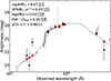 |
Fig. 15. Spectral energy distribution of the host galaxy of SN 2023gpw from 1000 to 60 000 Å(black points) and the best-fitting Prospector model (solid line). The red squares represent the model-predicted magnitudes; some deviation can be seen in the NUV. The fitting parameters are shown in the upper-left corner. The abbreviation “n.o.f.” stands for the number of filters. |
The absolute magnitude of the host galaxy in the optical is between −17.28 ± 0.05 (LS g band) and −17.89 ± 0.11 mag (LS z band). Assuming the g-band value is comparable to the B-band absolute magnitudes reported for the Kangas et al. (2022) sample, the host galaxy of SN 2023gpw would be somewhat fainter than the median (−18.7 mag) or the average (−17.9 mag). The host-galaxy extinction from the fit is very minor ( mag), less than 2σ from zero extinction. In terms of stellar mass (log
  ), the host is roughly average compared to other SLSN II hosts (Kangas et al. 2022); the star formation rate (
 M⊙ yr−1), though, is rather low. The host galaxy lies on the low-mass tail of the host galaxy distribution of normal SNe II at z > 0.08 (Schulze et al. 2021).
5. Discussion
5.1. Excluding the tidal disruption event scenario
Despite the (by eye) near-nuclear location of SN 2023gpw, we find a distance of ∼1.5 kpc or  between the centroid of the SN and the nucleus of the host galaxy (see Sect. 4.3), making a TDE origin for it highly unlikely. Nonetheless, as an additional check, we compared it to TDEs. The spectral features observed in SN 2023gpw are dominated by hydrogen and helium features early on, similar to the H+He class of TDEs (Arcavi et al. 2014; van Velzen et al. 2021), but several differences are apparent. The host galaxy itself is a blue, faint, star-forming spiral galaxy with a relatively weak nucleus, which is atypical for a TDE host galaxy – these tend to be post-merger green-valley galaxies with centrally concentrated stellar distributions (Hammerstein et al. 2021). TDEs generally show declining blackbody radii, roughly constant temperatures, and a relation between temperature and radius, T ∝ R−1/2 (van Velzen et al. 2020, 2021; Hammerstein et al. 2023), which clearly contradict the observed blackbody evolution of SN 2023gpw (see Fig. 13). The NUV excess seen in our SEDs is also abnormal for a TDE, where typically a single blackbody captures the optical and NUV evolution (e.g. van Velzen et al. 2020). We can therefore rule out a TDE origin for SN 2023gpw.
5.2. SN 2023gpw compared to other SLSNe II
Light-curve-wise, SN 2023gpw does not particularly stand out from other SLSNe II in the g band. It is among the more luminous objects of the class, but not extremely so; its luminosity places it close to the border of the “IIP/L-like” and “08es-like” subclasses among SLSNe II that Kangas et al. (2022) divide their sample into. While SN 2023gpw is initially somewhat hotter and bluer than other SLSNe II, this does not last very long. The host galaxy of SN 2023gpw does not stand out compared to those of other SLSNe II. In terms of these subgroups, the host is perhaps more similar to those of the “IIP/L-like” group, but the sample of “08es-like” SNe is small enough that the difference is not clear.
However, two things set SN 2023gpw apart. One is that in all other SLSNe II, the UV excess is visible at all observed epochs (Miller et al. 2009; Kangas et al. 2022), while in SN 2023gpw it appears between +4 and +18 d, when the blackbody temperature declines from 15 000 to 11 000 K. The extra emission may simply be less clear at higher temperatures where the blackbody peak coincides with it. The more important thing is the steepening light curve in the redder bands, possibly similar to normal SNe II where it signals the full recombination of the hydrogen and the transition to the radioactive tail. A steepening like this has not been observed in any other SLSN II, and can indeed be excluded in some, including the prototypical SN 2008es (Bhirombhakdi et al. 2019). A drop of multiple magnitudes is not necessarily related to recombination. Similar features can appear if the dominant energy input mechanism turns off; for example, in interacting SNe when the forward shock reaches the outer edge of the CSM (Khatami & Kasen 2024).
Out of the models included in MOSFiT that we applied in this study, only the CSI model replicates the light curve, including this steepening. This is in contrast to the samples of Inserra et al. (2018) and Kangas et al. (2022), where the magnetar model was either favored over the CSI model or was roughly equally effective when it comes to light curve fitting, though some signs of interaction were seen, such as a UV excess over a blackbody and/or late-time multi-component Hα profiles. Even in SN 2008es, Bhirombhakdi et al. (2019) could not exclude the magnetar model with a time-dependent gamma-ray trapping efficiency, though their late-time data favored the CSI model.
Multi-component “flash” features are not seen in most SLSNe II. In some cases, this can be simply because no early spectra exist, except possibly at very low resolution, and their existence at similar times since the explosion cannot often be excluded. In the combined Inserra et al. (2018) and Kangas et al. (2022) sample, SNe 2019zcr, 2019aanx, and 2020bfe have pre-peak spectra (−16, −11, and −14 d respectively) with a possibly multi-component line profile of Hα as in SN 2023gpw, but He IIλ4868 is not seen in any spectrum. The earliest spectra of SN 2008es in Gezari et al. (2009) do show a He IIλ4868 as well as Hα at ∼ − 10 d, but neither has a narrow component.
The later photospheric spectra show some differences from other SLSNe II as well. The spectra of SN 2008es (Fig. 9), and by extension other 2008es-like SNe (Kangas et al. 2022), show broader and more symmetric Hα profiles but similar metal (iron?) lines in the blue part of the spectrum. Meanwhile, several SLSNe II show spectra similar to somewhat less luminous SNe II (Fig. 10), either normal SNe II with P Cygni line profiles or interacting SNe II such as SN 1979C (Panagia et al. 1980) and SN 1998S (Fassia et al. 2001). The objects without clear P Cygni profiles in Hα still often have other typical SN II features, such as clearly skewed Hα profiles with suppressed wings, Ca II NIR triplet emission and/or strong Na I + He I absorption, none of which are clearly seen in SN 2023gpw. The peak luminosity of SN 2023gpw is on the borderline between these two subgroups as stated above, and its spectra show similarity to both groups but have no exact match among other SLSNe II.
The polarization of only one SLSN II has been measured previously: Inserra et al. (2018) obtained an early polarization degree of p = (0.94 ± 0.17)% for PS15br, implying an asymmetry of 10–15% assuming an ellipsoidal photosphere; however, the authors note that it is difficult to distinguish whether the polarization is intrinsic to PS15br or interstellar. The polarization degree in SN 2023gpw is consistent with this, p = (0.66 ± 0.33)% (see Sect. 3.3); though it is only 2σ from zero. Similar pre-peak numbers have also been seen in SLSNe I (Pursiainen et al. 2023). As a comparison, Leonard et al. (2000) found a pre-peak 2% polarization in SN 1998S, which was implied to have a disk-like CSM because of the polarization and multi-peaked line profiles. Nagao et al. (2024), on the other hand, found polarization degrees of ≲1.2% in the photospheric phases of normal SNe II; often the polarization increases in the tail phase, revealing asymmetries in the inner ejecta. In a similar vein, the late-time Hα profiles of PS15br and SN 2013hx had multiple components, implying asymmetric CSM (Inserra et al. 2018). We cannot say whether either kind of evolution occurs in SN 2023gpw.
5.3. Asymmetry and evolution of the photosphere
In the spectra, as discussed in Sect. 3.2, we see “flash” emission lines of the Balmer series and He IIλ4686. At the epoch of our polarization measurement, these lines are still visible on top of an otherwise featureless continuum. Therefore, the photosphere is – at least partially – within the CSM and does not necessarily reflect the shape of the ejecta. The CSM seems to be only slightly aspherical, but unfortunately, this too is difficult to say for certain, as it depends on the angle of the ISP and the viewing angle. However, there is another sign of asymmetry in the ejecta. The velocity of the Hα emission and He Iλ5876 absorption in the ejecta is lower than that of the photosphere from the blackbody fits by about a factor of two. This suggests an aspherical, possibly bipolar ejecta, in which case an observer at some viewing angles could see lower velocities in the radial than the transverse direction (lines vs. photosphere expansion).
The expansion of the photosphere, according to our blackbody fits, does not appreciably decelerate, and is instead fairly constant at ∼9100 km s−1 until ≳55 d after the peak, indicating that the photosphere does not recede below an outer ejecta layer for a long time. In our line of sight, this layer corresponds to a much lower velocity (∼4500 km s−1) because of the asymmetry of the ejecta. For the photosphere to stay at a constant velocity throughout our observations and even before the peak, the ejecta requires a relatively sharp outer edge – this could also result in a weak P Cygni absorption in Hα (Schlegel 1996). Analogously to a normal SN II, the opacity of the ejecta can drop dramatically after cooling below the recombination temperature, which is almost reached in our blackbody fits; this can cause a drop in the light curve as the photosphere finally recedes.
5.4. CSM interaction
The flash features in SN 2023gpw are, in broad strokes, similar to those seen in normal SNe II (e.g. Bruch et al. 2021, 2023), as they consist of a narrow component with broad wings attributed to electron scattering, which weaken over time and disappear between the peak and +12 d, when the He IIλ4686 seems to have been replaced by a P Cygni profile of He Iλ5876. Thus, with our constraints on the explosion date (within a few days of the discovery according to MOSFiT), we can say that these lines disappear roughly between 32 and 45 days after the explosion. Assuming the disappearance of the lines is because the SN ejecta catches up to and sweeps up the CSM where they originate, the ejecta velocity (∼9100 km s−1) we estimate based on the expansion of the blackbody radius (see Sect. 4.1) leads to an extent of between 2.5 × 10¹⁵ and 3.5 × 1015 cm for this “confined” CSM. We note, though, that the radius of the blackbody was calculated assuming a spherical photosphere, and thus the velocity can be considered an average over all solid angles. Along the line of sight, the velocity is smaller by about a factor of two, and thus the extent of the CSM can be closer to ∼1.5 ×1015 cm. In many SNe II, flash features tend to disappear in a few to several days (Khazov et al. 2016; Bruch et al. 2021; Jacobson-Galán et al. 2024) implying an extent of < 1015 cm for the confined CSM assuming a representative ejecta velocity of 10 000 km s−1; though we note that the recent, well-observed SN 2023ixf exhibited narrow lines until ∼15 d (Zimmerman et al. 2024). In any case, such features last relatively long in SN 2023gpw, and the CSM responsible for them seems more extended than in normal SNe II.
The disappearance of the flash features does not indicate the end of all CSI. After this time, the lack of narrow lines could in principle be due to any strong interaction being hidden behind the ejecta photosphere if, for example, the ejecta overruns an aspherical, possibly disk-like CSM (e.g. Smith et al. 2015). In this case, the CSI would keep contributing to the luminosity without narrow lines. An aspherical interaction region within the ejecta should result in an aspherical photosphere, as our velocity discrepancy indicates (e.g. Smith 2017). Again, the ISP and the viewing angle have an effect on the resulting polarization. Alternatively, an optically thick CSM with a sharp outer edge could explain the lack of narrow lines (Moriya & Tominaga 2012). In this case, only a small part of the CSM near the outer edge is optically thin. Narrow lines in the spectrum would only appear in this scenario while the shock is in the optically thin outer part of the CSM, leading to events apparently without strong narrow lines if this part is thin. In the case of SN 2023gpw, we could see narrow lines with electron-scattering wings from the outer layers of this CSM until they are shocked by the ejecta.
One signature of CSI we see after the flash features disappear is the UV excess in the form of a flat NUV spectrum (see Sect. 4.1). A UV excess is also seen in all SLSNe II with UV data shown in Kangas et al. (2022), and in some other, less luminous SNe II such as SN 1979C (Panagia et al. 1980) and SN 2023ixf (Bostroem et al. 2024)13. In SN 2023gpw, this excess appears a few weeks after the peak – about the same time as the broad emission lines. The epoch when the excess appears was missed in the objects shown by Kangas et al. (2022), but in SN 2008es, the excess predates the broad lines (Miller et al. 2009). To create such an excess, one needs a source of UV photons that are not reprocessed in the ejecta and therefore originate outside the photosphere, making CSI an obvious candidate. If UV photons can escape, a large portion of CSI energy is indeed expected to emerge in the UV (e.g., Fransson 1984; Dessart & Hillier 2022). However, the excess could be created through weaker interaction with a more tenuous outer CSM, to which the UV is more sensitive than the optical (Bostroem et al. 2024). In fact, in some strongly interacting SNe, such as SN 2013L (Taddia et al. 2020), a clear UV excess is not seen, likely because the UV photons are thermalized while the forward shock is still in the dense CSM.
We therefore propose that, early on, before and around the peak of the light curve, CSI occurs between the ejecta and a dense, slightly asymmetric, CSM confined to within a few ×1015 cm. An extended envelope is also a possibility, but this radius (≳15 000 R⊙) surpasses the radii of quiescent supergiant stars by an order of magnitude (Levesque 2017). The peak of the light curve in this scenario is expected to nearly coincide with the emergence of the shock from within the optically thick part of the CSM (Moriya & Tominaga 2012), which is consistent with our observations. Further out, there is a more tenuous CSM, and further interaction with it creates the UV excess.
If interaction with a dense CSM or an extended envelope occurs during the rise, the early photosphere should exhibit at least the radius of the optically thick part of the CSM/envelope and an increasing temperature. The earliest blackbody fits are indeed consistent with this expectation, but not very robust as they are based on only two or three optical bands. Any significant deceleration of the expansion of the photosphere (necessary if bulk deceleration of the ejecta is significant) would result in the constant-velocity line (Fig. 13) intersecting zero radius before the explosion, which is not the case. The implication is that, despite the interaction, significant deceleration does not occur in the bulk of the ejecta, and therefore the CSM mass is small compared to the ejecta – though deceleration can occur in outer layers that are initially faster than ∼9000 km s−1.
We can roughly estimate the mass-loss rate from the peak pseudo-bolometric luminosity, Lpeak, of the SN using the following relation (e.g. Smith 2017), assuming the luminosity at this point is dominated by interaction:
 (1)
(1)
where vCSM is the CSM velocity and vej the ejecta velocity. We note that the luminosity is pseudo-bolometric, which underestimates the mass loss, but at the same time the assumption of being dominated by interaction may overestimate it. We first assume that the width of the narrower emission component of Hα, intrinsically roughly 700 km s−1, corresponds to the velocity of material ejected previously (i.e., vCSM = 700 km s−1). With Lpeak ∼ 2.8 × 1044 erg s−1 and ϵ = 0.5, we obtain  . This rate is somewhat extreme, but perhaps plausible in a luminous blue variable (LBV) giant eruption (Smith 2014). With the radius of the confined CSM (a few ×1015 cm) we obtain from the timing of the flash features, the mass loss responsible for that CSM would have happened on the order of a year before the SN explosion. If, however, this component is created through electron scattering in unshocked CSM, we can instead assume a velocity more typical for the wind of an LBV, vCSM = 100 km s−1 (Smith 2017), which is also closer to the narrow lines we see at +29 and +43 d. Doing so, we obtain
  and a timing within several years of the SN.
5.5. The power source and progenitor of SN 2023gpw
As stated above, the MOSFiT magnetar or (continuous) fallback models seem to fail to reproduce the light curve of SN 2023gpw and the steepening in the light curve (see Sect. 4.2). The obvious conclusion of this would be to favor the CSI model, which can replicate the observed light curve especially with s = 0. However, in the CSI scenario, the energy source is ultimately the kinetic energy of the ejecta, regulated by the efficiency of the conversion of this energy into radiation, ϵ (Dessart et al. 2015, as an example, a range of 0.3 to 0.7 for ϵ is seen in simulations by][with higher CSM-to-ejecta mass ratios resulting in more efficiency). In SN 2023gpw, similarly to the few most luminous objects in Kangas et al. (2022), the total radiated energy is on the order of 1051 erg. This may represent a problem for the neutrino-driven CCSN mechanism, as neutrino-driven simulations are unable to exceed ∼2 × 1051 erg (Janka 2012). If it does, another power source, such as a central engine, may also be required.
In our case, a neutrino-driven SN would require on the order of ≳45% of the total kinetic energy to be converted to reproduce the radiated energy of ≳8.9 × 1050 erg we estimate (see Sect. 3.1), which is, in itself, not necessarily a problem in the CSI model, but would cause significant deceleration in the ejecta (by a few thousand km s−1). It is possible that, if the CSM is very asymmetric, such deceleration does occur along the line of sight while most of the ejecta expands unimpeded. This would, however, mean that a large fraction of the ejecta does not take part in the interaction, and that the kinetic energy again becomes a problem; a neutrino-driven explosion would require at least 60% of the ejecta to decelerate to 5000 km s−1. It is more likely that the ejecta itself is asymmetric to begin with.
Next, we attempted to estimate an ejecta mass for SN 2023gpw based on the rise time of the light curve using the equation
 (2)
(2)
where τm is the diffusion timescale, β ≈ 13.8 is an integration constant, and v is a scaling velocity for homologous expansion (Arnett 1980, 1982). We fixed κ at 0.34 cm2 g−1 as before. We approximated the diffusion timescale as the rise time, ∼30 d, and the scaling velocity as the expansion velocity of the blackbody photosphere. The resulting ejecta mass is ∼3 M⊙. With this mass and the blackbody expansion velocity, the estimated kinetic energy would be  erg. Here the radiated energy would be on the order of ≳60% of the kinetic energy, which is again problematic.
This is an indication that the Arnett formula, which assumes a central power source and diffusion through the whole ejecta, is inapplicable to SN 2023gpw, as the diffusion only occurs outward from the interaction region, and the true ejecta mass is likely much larger. If only a small fraction of the total kinetic energy is emitted, it must be at least several ×1051 erg, which, at a velocity of 9100 km s−1, translates to a mass at least on the order of 10 M⊙. This rough lower limit is compatible with our fitting results with the csm model. However, we note that the CSM mass in the s = 0 fit is large compared to the ejecta mass, which is unlikely if the CSM is symmetric but a large fraction of the kinetic energy is not emitted. Furthermore, fits using the csm model cannot account for any asymmetry. As an order-of-magnitude estimate, the ejecta mass in the s = 2 fit is  M⊙, resulting in Ek ∼ 1.4 × 1052 erg. In this case, the fraction of total kinetic energy converted to radiation would only be ∼0.05.
If energies in excess of a neutrino-driven SN are required, we must consider the magnetar spin-down model. At first glance, a magnetar power source is disfavored by the MOSFiT modeling (Sect. 4.2) because of the drop in the red bands of the light curve. The generalized magnetar model of Omand & Sarin (2024) similarly cannot reproduce this drop. Magnetar models specifically constructed for hydrogen-rich SLSNe, however, can produce a plateau and a drop analogous to normal SNe II with some parameters (Orellana et al. 2018). One can, alternatively, obtain intermediate cases with a short plateau phase and a drop in the (bolometric) light curve or a smoother light curve with no drop. Notably, some of these models also re-create the observed constant photospheric velocity, as most of the ejecta is pushed from within into a dense shell that it takes a long time for the photosphere to recede through.
We note that other simulations do not necessarily agree. In models of magnetar-powered SLSNe II by Dessart & Audit (2018), the same qualitative light curve shapes with plateaus can be generated, but while the influence of a magnetar does slow down the photospheric velocity decline, it is too steep for SN 2023gpw nonetheless. In three-dimensional magnetar-driven SN simulations by Suzuki & Maeda (2019), the ejecta is also being pushed from the inside, but the hot, fast magnetar wind breaks through it, resulting in a thick, clumpy dense ejecta instead of a thin shell, with a relatively shallow outer density profile. This could explain the UV excess, but seems incompatible with the constant photospheric velocity. However, Suzuki & Maeda (2019) do not include radiative transfer in their simulation and note that doing this might suppress the breakout.
The decline of the pseudo-bolometric light curve of SN 2023gpw only slows down slightly before the solar conjunction, with no plateau, but, during the gap, presumably steepens as the red bands do. This is still qualitatively similar to the intermediate models of Orellana et al. (2018). Another problem, however, is that the aforementioned models have no early CSI. SN 2023gpw is more luminous at peak than any model shown by Orellana et al. (2018) or Dessart & Audit (2018), by a factor of a few, and declines faster, which could be attributed to CSI analogously to a normal SN II (Morozova et al. 2017). We also note that the models discussed here form a sparse grid, with the ejecta mass fixed at 10 M⊙ in the Orellana et al. (2018) and Suzuki & Maeda (2019) simulations and either 11.9 or 15.6 M⊙ in Dessart & Audit (2018). It is possible that by adjusting the parameters and taking into account the early CSI, the observed properties could be reproduced. We encourage modeling this scenario in further detail, including multi-band light curves, to determine whether it is applicable. We also note that these simulations assume spherical symmetry for the ejecta and the spin-down energy input, which seems to be disfavored by our observations.
If the ejecta mass in SN 2023gpw can be on the order of 30 M⊙, there is a possibility of an extremely massive progenitor star, and a pulsational pair-instability SN (PPISN; Woosley 2017) scenario should be discussed. A star with a helium core of 35–65 M⊙ can experience pair instability that does not fully unbind the star, but instead proceeds in pulses (hence pulsational pair instability, or PPI) that eject large amounts of mass. Transients from such objects can include the mass ejections themselves, collisions between CSM shells, or the final SN at the end of such a star’s life – if one can happen – plus CSI. However, Woosley (2017) states that a SLSN is difficult to produce with PPI. The radiated energy from PPISN models is not expected to exceed 5 × 1050 erg, and shell velocities should be much lower than the blackbody velocity observed in SN 2023gpw.
After PPI, the core is unlikely to explode as an SN, but it might do so in a collapsar-like scenario (see also Woosley 1993). Woosley (2017) brings up a situation where after PPI, the core partially collapses into a black hole and accretion onto it powers a bipolar outflow, which, similarly to the magnetar central engine, can then interact with the previously ejected mass and artificially condense the ejecta from the inside. The accretion could produce a kinetic energy in excess of 1052 erg, as is often seen in broad-lined SNe Ic (SNe Ic-BL) accompanying gamma-ray bursts (GRBs), also the products of collapsars (e.g. Woosley et al. 1999). Other SNe Ic-BL can also exhibit similar energies even without a GRB (e.g. Taddia et al. 2019), if a relativistic jet does not break out of the ejecta. Whether the progenitor star experienced PPI or not, a black hole as the central engine may explain SN 2023gpw. The MOSFiT fallback model suffers from the same late-time problem as the magnetar model, but it assumes continuous accretion. If, instead, accretion turns off after some time, a steepening decline can be accommodated.
6. Conclusions
We have presented photometric and spectroscopic follow-up observations and analysis of SN 2023gpw, a SLSN II with early “flash" emission lines and later dominated by broad spectral lines. We performed blackbody and light curve modeling and compared SN 2023gpw to other SLSNe II. Our conclusions are as follows:
-
With a rise time of
 d and a g-band peak absolute magnitude of Mg, peak = −21.58 ± 0.03 mag, SN 2023gpw is a relatively fast-rising SLSN II, but neither its luminosity nor its rise time are unprecedented among SLSNe II. Its host galaxy is fainter and less massive than most SN II hosts but normal for a SLSN II host.
 -
The UV photometry exhibits an excess over a blackbody, which is so far ubiquitous among SLSNe II and also seen in some normal SNe II. However, SN 2023gpw is so far the only SLSN II where its appearance, coinciding with that of the broad spectral lines, is documented.
-
When ignoring the bluest UV data after the peak, the blackbody radius expands at a constant velocity of ∼9100 km s−1. Extrapolation of this velocity to earlier epochs results in a zero radius close to the explosion date (∼ − 30 d), indicating no significant bulk deceleration in the ejecta throughout the observed evolution. The photosphere does not seem to recede past the outer ejecta until ≳ + 50 d.
-
The light curve indicates an abrupt drop of several magnitudes in the red bands during a solar conjunction, between ∼ + 80 and ∼ + 180 d, after which the SN is no longer detected. This is unprecedented among SLSNe II and may correspond to the epoch when the photosphere finally recedes into lower-velocity ejecta.
-
The flash features, their disappearance around the light curve peak, and the later UV excess indicate interaction with a dense, confined CSM early on followed by ongoing weaker interaction with a more tenuous CSM.
-
Likely polarization at p = (0.66 ± 0.33)% is observed during the early interaction, suggesting a slightly aspherical CSM and/or an aspherical ejecta interacting with it. The discrepancy in expansion velocities measured from the blackbody fits and from the spectral lines also indicates asymmetry.
-
The total radiation emitted by SN 2023gpw is estimated as ≳8.9 × 1050 erg, which in a normal neutrino-driven SN would require a large fraction of the total kinetic energy to be converted to emission. However, due to the lack of bulk deceleration, the observed interaction is unlikely to result in such an efficient conversion. Instead, it is likely that the kinetic energy is on the order of 1052 erg, and the ejecta mass is therefore ≳10 M⊙.
-
The light curve drop is not reproduced by the magnetar model in MOSFiT. The light curve and constant photospheric velocity are, however, qualitatively similar to some models of magnetar-powered hydrogen-rich SLSNe (Orellana et al. 2018), but more modeling work is required to determine if this scenario, combined with early interaction, can reproduce the full light curve.
-
Another scenario for producing the required kinetic energy and ejecta mass is one where the core of a very massive progenitor star, possibly after PPI episodes that produce the CSM, collapses into a black hole. Fall-back accretion onto this black hole then results in a bipolar outflow heating the ejecta from the inside until the accretion stops, causing the drop in brightness
A handful of SLSNe II exhitibiting extreme energy requirements, including SN 2023gpw, seem to require a central engine in addition to interaction. Whether this engine is the same for all objects of this type is still unclear, as is whether some less extreme SLSNe II are also powered by a central engine. By exhibiting properties previously unseen within this group, SN 2023gpw provides some hints about these issues, but does not resolve them. A larger sample of well-observed SLSNe II, including constraints on asymmetry and late-time behavior, may shed light on these issues over time.
Data availability
All spectra presented in this paper are available for download on WISEREP (Yaron & Gal-Yam 2012) at https://www.wiserep.org/object/23362.
SN 2020yue does not show such an excess, but this object was later re-classified a TDE by Yao et al. (2023).
Foscgui is a graphic user interface aimed at extracting SN spectroscopy and photometry obtained with FOSC-like instruments. It was developed by E. Cappellaro. A package description can be found at http://sngroup.oapd.inaf.it/foscgui.html.
Acknowledgments
We thank the anonymous referee for useful comments, and Georgios Dimitriadis for re-reducing the INT spectrum. T.K. acknowledges support from the Research Council of Finland project 360274. R.K. and T.L.K. acknowledge support from the Research Council of Finland (340613). M.S. is funded by the Independent Research Fund Denmark (IRFD) via Project 2 grant 10.46540/2032-00022B and by the Aarhus University Nova grant# AUFF-E-2023-9-28. N.E.R. acknowledges support from the PRIN-INAF 2022, ‘Shedding light on the nature of gap transients: from the observations to the models’ and from the Spanish Ministerio de Ciencia e Innovación (MCIN) and the Agencia Estatal de Investigación (AEI) 10.13039/501100011033 under the program Unidad de Excelencia María de Maeztu CEX2020-001058-M. C.P.G. acknowledges financial support from the Secretary of Universities and Research (Government of Catalonia) and by the Horizon 2020 Research and Innovation Programme of the European Union under the Marie Skłodowska-Curie and the Beatriu de Pinós 2021 BP 00168 programme, from the Spanish Ministerio de Ciencia e Innovación (MCIN) and the Agencia Estatal de Investigación (AEI) 10.13039/501100011033 under the PID2023-151307NB-I00 SNNEXT project, from Centro Superior de Investigaciones Científicas (CSIC) under the PIE project 20215AT016 and the program Unidad de Excelencia María de Maeztu CEX2020-001058-M, and from the Departament de Recerca i Universitats de la Generalitat de Catalunya through the 2021-SGR-01270 grant. T.L.K. acknowledges a Warwick Astrophysics prize post-doctoral fellowship made possible thanks to a generous philanthropic donation. T.E.M.B. is funded by Horizon Europe ERC grant no. 101125877. The Starlink software (Currie et al. 2014) is currently supported by the East Asian Observatory. This study is based on observations made with the Gran Telescopio Canarias (GTC), installed in the Spanish Observatorio del Roque de los Muchachos of the Instituto de Astrofísica de Canarias, in the island of La Palma. Access to the Las Cumbres Observatory was made possible via an allocation by OPTICON (program 22A/012, PI Stritzinger). This project has received funding from the European Union’s Horizon 2020 research and innovation programme under grant agreement No 101004719. Based on observations obtained with the Samuel Oschin Telescope 48-inch and the 60-inch Telescope at the Palomar Observatory as part of the Zwicky Transient Facility project. ZTF is supported by the National Science Foundation under Grant No. AST-2034437 and a collaboration including Caltech, IPAC, the Weizmann Institute of Science, the Oskar Klein Center at Stockholm University, the University of Maryland, Deutsches Elektronen-Synchrotron and Humboldt University, the TANGO Consortium of Taiwan, the University of Wisconsin at Milwaukee, Trinity College Dublin, Lawrence Livermore National Laboratories, IN2P3, University of Warwick, Ruhr University Bochum, Cornell University, and Northwestern University. Operations are conducted by COO, IPAC, and UW.
References
- Abdurro’uf, Accetta, K., Aerts, C., et al. 2022, ApJS, 259, 35 [NASA ADS] [CrossRef] [Google Scholar]
- Alard, C. 2000, A&AS, 144, 363 [NASA ADS] [CrossRef] [EDP Sciences] [Google Scholar]
- Alard, C., & Lupton, R. H. 1998, ApJ, 503, 325 [Google Scholar]
- Ambikasaran, S., Foreman-Mackey, D., Greengard, L., Hogg, D. W., & O’Neil, M. 2015, IEEE Trans. Pattern Anal. Mach. Intell., 38, 252 [Google Scholar]
- Angus, C. R., Levan, A. J., Perley, D. A., et al. 2016, MNRAS, 458, 84 [NASA ADS] [CrossRef] [Google Scholar]
- Arcavi, I., Gal-Yam, A., Sullivan, M., et al. 2014, ApJ, 793, 38 [Google Scholar]
- Arnett, W. D. 1980, ApJ, 237, 541 [Google Scholar]
- Arnett, W. D. 1982, ApJ, 253, 785 [Google Scholar]
- Barkat, Z., Rakavy, G., & Sack, N. 1967, Phys. Rev. Lett., 18, 379 [Google Scholar]
- Bellm, E. C., Kulkarni, S. R., Graham, M. J., et al. 2019, PASP, 131, 018002 [Google Scholar]
- Benetti, S., Nicholl, M., Cappellaro, E., et al. 2014, MNRAS, 441, 289 [CrossRef] [Google Scholar]
- Bennett, C. L., Larson, D., Weiland, J. L., & Hinshaw, G. 2014, ApJ, 794, 135 [Google Scholar]
- Bhirombhakdi, K., Chornock, R., Miller, A. A., et al. 2019, MNRAS, 488, 3783 [NASA ADS] [CrossRef] [Google Scholar]
- Blagorodnova, N., Neill, J. D., Walters, R., et al. 2018, PASP, 130, 035003 [Google Scholar]
- Bostroem, K. A., Sand, D. J., Dessart, L., et al. 2024, ApJ, 973, L47 [NASA ADS] [CrossRef] [Google Scholar]
- Bradley, L., Sipőcz, B., Robitaille, T., et al. 2024, https://doi.org/10.5281/zenodo.596036 [Google Scholar]
- Brown, T. M., Baliber, N., Bianco, F. B., et al. 2013, PASP, 125, 1031 [Google Scholar]
- Bruch, R. J., Gal-Yam, A., Schulze, S., et al. 2021, ApJ, 912, 46 [NASA ADS] [CrossRef] [Google Scholar]
- Bruch, R. J., Gal-Yam, A., Yaron, O., et al. 2023, ApJ, 952, 119 [NASA ADS] [CrossRef] [Google Scholar]
- Byler, N., Dalcanton, J. J., Conroy, C., & Johnson, B. D. 2017, ApJ, 840, 44 [Google Scholar]
- Calzetti, D., Armus, L., Bohlin, R. C., et al. 2000, ApJ, 533, 682 [NASA ADS] [CrossRef] [Google Scholar]
- Chabrier, G. 2003, PASP, 115, 763 [Google Scholar]
- Chambers, K. C., Magnier, E. A., Metcalfe, N., et al. 2016, ArXiv e-prints [arXiv:1612.05560] [Google Scholar]
- Chatzopoulos, E., Wheeler, J. C., Vinko, J., Horvath, Z. L., & Nagy, A. 2013, ApJ, 773, 76 [NASA ADS] [CrossRef] [Google Scholar]
- Chen, Z. H., Yan, L., Kangas, T., et al. 2023a, ApJ, 943, 41 [NASA ADS] [CrossRef] [Google Scholar]
- Chen, Z. H., Yan, L., Kangas, T., et al. 2023b, ApJ, 943, 42 [NASA ADS] [CrossRef] [Google Scholar]
- Chevalier, R. A., & Fransson, C. 1994, ApJ, 420, 268 [NASA ADS] [CrossRef] [Google Scholar]
- Chugai, N. N., & Utrobin, V. P. 2022, MNRAS, 512, L71 [NASA ADS] [CrossRef] [Google Scholar]
- Conroy, C., Gunn, J. E., & White, M. 2009, ApJ, 699, 486 [Google Scholar]
- Currie, M. J., Berry, D. S., Jenness, T., et al. 2014, ASP Conf. Ser., 485, 391 [Google Scholar]
- Dekany, R., Smith, R. M., Riddle, R., et al. 2020, PASP, 132, 038001 [NASA ADS] [CrossRef] [Google Scholar]
- Dessart, L., & Audit, E. 2018, A&A, 613, A5 [Google Scholar]
- Dessart, L., & Hillier, D. J. 2022, A&A, 660, L9 [NASA ADS] [CrossRef] [EDP Sciences] [Google Scholar]
- Dessart, L., Audit, E., & Hillier, D. J. 2015, MNRAS, 449, 4304 [Google Scholar]
- Dexter, J., & Kasen, D. 2013, ApJ, 772, 30 [NASA ADS] [CrossRef] [Google Scholar]
- Dey, A., Schlegel, D. J., Lang, D., et al. 2019, AJ, 157, 168 [Google Scholar]
- Faran, T., Nakar, E., & Poznanski, D. 2018, MNRAS, 473, 513 [NASA ADS] [CrossRef] [Google Scholar]
- Fassia, A., Meikle, W. P. S., Chugai, N., et al. 2001, MNRAS, 325, 907 [NASA ADS] [CrossRef] [Google Scholar]
- Flewelling, H. A., Magnier, E. A., Chambers, K. C., et al. 2020, ApJS, 251, 7 [NASA ADS] [CrossRef] [Google Scholar]
- Foreman-Mackey, D., & Sick, J. 2014, Johnson, B., DOI 10.5281/zenodo.12157 [Google Scholar]
- Foreman-Mackey, D., Hogg, D. W., Lang, D., & Goodman, J. 2013, PASP, 125, 306 [Google Scholar]
- Förster, F., Cabrera-Vives, G., Castillo-Navarrete, E., et al. 2021, AJ, 161, 242 [CrossRef] [Google Scholar]
- Förster, F., Bauer, F. E., Pignata, G., et al. 2023, Transient Name Server Discovery Report, 2023–887, 1 [Google Scholar]
- Fransson, C. 1984, A&A, 133, 264 [NASA ADS] [Google Scholar]
- Fremling, C., Sollerman, J., Taddia, F., et al. 2016, A&A, 593, A68 [NASA ADS] [CrossRef] [EDP Sciences] [Google Scholar]
- Gal-Yam, A. 2012, Science, 337, 927 [Google Scholar]
- Gal-Yam, A. 2019, ARA&A, 57, 305 [Google Scholar]
- Gezari, S., Halpern, J. P., Grupe, D., et al. 2009, ApJ, 690, 1313 [NASA ADS] [CrossRef] [Google Scholar]
- Gomez, S., Nicholl, M., Berger, E., et al. 2024, MNRAS, 535, 471 [NASA ADS] [CrossRef] [Google Scholar]
- Gordon, K. D., Clayton, G. C., Decleir, M., et al. 2023, ApJ, 950, 86 [CrossRef] [Google Scholar]
- Graham, M. J., Kulkarni, S. R., Bellm, E. C., et al. 2019, PASP, 131, 078001 [Google Scholar]
- Guillochon, J., Nicholl, M., Villar, V. A., et al. 2018, ApJS, 236, 6 [NASA ADS] [CrossRef] [Google Scholar]
- Güver, T., & Özel, F. 2009, MNRAS, 400, 2050 [Google Scholar]
- Hammerstein, E., Gezari, S., van Velzen, S., et al. 2021, ApJ, 908, L20 [NASA ADS] [CrossRef] [Google Scholar]
- Hammerstein, E., van Velzen, S., Gezari, S., et al. 2023, ApJ, 942, 9 [NASA ADS] [CrossRef] [Google Scholar]
- Heger, A., & Woosley, S. E. 2002, ApJ, 567, 532 [Google Scholar]
- Heiles, C. 2000, AJ, 119, 923 [Google Scholar]
- Henden, A., & Munari, U. 2014, Contrib. Astron. Obs. Skalnate Pleso, 43, 518 [NASA ADS] [Google Scholar]
- Hiramatsu, D., Berger, E., Gomez, S., et al. 2024, ApJ, submitted [arXiv:2411.07287] [Google Scholar]
- Hogg, D. W., Baldry, I. K., Blanton, M. R., & Eisenstein, D. J. 2002, ArXiv e-prints [arXiv:astro-ph/0210394] [Google Scholar]
- Hosseinzadeh, G., Berger, E., Metzger, B. D., et al. 2022, ApJ, 933, 14 [NASA ADS] [CrossRef] [Google Scholar]
- Inserra, C., Smartt, S. J., Jerkstrand, A., et al. 2013, ApJ, 770, 128 [NASA ADS] [CrossRef] [Google Scholar]
- Inserra, C., Nicholl, M., Chen, T. W., et al. 2017, MNRAS, 468, 4642 [NASA ADS] [CrossRef] [Google Scholar]
- Inserra, C., Smartt, S. J., Gall, E. E. E., et al. 2018, MNRAS, 475, 1046 [NASA ADS] [CrossRef] [Google Scholar]
- Jacobson-Galán, W. V., Dessart, L., Davis, K. W., et al. 2024, ApJ, 970, 189 [CrossRef] [Google Scholar]
- Janka, H.-T. 2012, Ann. Rev. Nucl. Part. Sci., 62, 407 [Google Scholar]
- Jiang, B., Jiang, S., & Ashley Villar, V. 2020, Res. Notes Am. Astron. Soc., 4, 16 [Google Scholar]
- Kangas, T., Yan, L., Schulze, S., et al. 2022, MNRAS, 516, 1193 [Google Scholar]
- Kasen, D., & Bildsten, L. 2010, ApJ, 717, 245 [NASA ADS] [CrossRef] [Google Scholar]
- Khatami, D. K., & Kasen, D. N. 2024, ApJ, 972, 140 [NASA ADS] [CrossRef] [Google Scholar]
- Khazov, D., Yaron, O., Gal-Yam, A., et al. 2016, ApJ, 818, 3 [CrossRef] [Google Scholar]
- Kim, Y. L., Rigault, M., Neill, J. D., et al. 2022, PASP, 134, 024505 [NASA ADS] [CrossRef] [Google Scholar]
- Kravtsov, T., Hueichapan, E., Wiseman, P., et al. 2023, Transient Name Server AstroNote, 165, 1 [Google Scholar]
- Lang, D. 2014, AJ, 147, 108 [Google Scholar]
- Leja, J., Johnson, B. D., Conroy, C., van Dokkum, P. G., & Byler, N. 2017, ApJ, 837, 170 [NASA ADS] [CrossRef] [Google Scholar]
- Leloudas, G., Maund, J. R., Gal-Yam, A., et al. 2017, ApJ, 837, L14 [NASA ADS] [CrossRef] [Google Scholar]
- Leonard, D. C., Filippenko, A. V., Barth, A. J., & Matheson, T. 2000, ApJ, 536, 239 [Google Scholar]
- Levesque, E. M. 2017, Astrophysics of Red Supergiants [Google Scholar]
- Lunnan, R., Chornock, R., Berger, E., et al. 2016, ApJ, 831, 144 [NASA ADS] [CrossRef] [Google Scholar]
- Lunnan, R., Fransson, C., Vreeswijk, P. M., et al. 2018, Nat. Astron., 2, 887 [NASA ADS] [CrossRef] [Google Scholar]
- Mainzer, A., Bauer, J., Cutri, R. M., et al. 2014, ApJ, 792, 30 [Google Scholar]
- Masci, F. J., Laher, R. R., Rusholme, B., et al. 2019, PASP, 131, 018003 [Google Scholar]
- Meisner, A. M., Lang, D., & Schlegel, D. J. 2017, AJ, 153, 38 [Google Scholar]
- Miller, A. A., Chornock, R., Perley, D. A., et al. 2009, ApJ, 690, 1303 [NASA ADS] [CrossRef] [Google Scholar]
- Moriya, T. J. 2026, Encyclopedia Astrophys., 2, 720 [Google Scholar]
- Moriya, T. J., & Tominaga, N. 2012, ApJ, 747, 118 [Google Scholar]
- Moriya, T. J., Nicholl, M., & Guillochon, J. 2018, ApJ, 867, 113 [NASA ADS] [CrossRef] [Google Scholar]
- Moriya, T. J., Murase, K., Kashiyama, K., & Blinnikov, S. I. 2022, MNRAS, 513, 6210 [NASA ADS] [CrossRef] [Google Scholar]
- Morozova, V., Piro, A. L., & Valenti, S. 2017, ApJ, 838, 28 [NASA ADS] [CrossRef] [Google Scholar]
- Morozova, V., Piro, A. L., & Valenti, S. 2018, ApJ, 858, 15 [Google Scholar]
- Nadyozhin, D. K. 1994, ApJS, 92, 527 [Google Scholar]
- Nagao, T., Patat, F., Cikota, A., et al. 2024, A&A, 681, A11 [NASA ADS] [CrossRef] [EDP Sciences] [Google Scholar]
- Nagy, A. P. 2018, ApJ, 862, 143 [Google Scholar]
- Nicholl, M. 2018, Res. Notes Am. Astron. Soc., 2, 230 [NASA ADS] [Google Scholar]
- Nicholl, M., Smartt, S. J., Jerkstrand, A., et al. 2015, MNRAS, 452, 3869 [NASA ADS] [CrossRef] [Google Scholar]
- Nicholl, M., Guillochon, J., & Berger, E. 2017, ApJ, 850, 55 [NASA ADS] [CrossRef] [Google Scholar]
- Ofek, E. O., Cameron, P. B., Kasliwal, M. M., et al. 2007, ApJ, 659, L13 [CrossRef] [Google Scholar]
- Oke, J. B., & Gunn, J. E. 1982, PASP, 94, 586 [Google Scholar]
- Oke, J. B., & Gunn, J. E. 1983, ApJ, 266, 713 [NASA ADS] [CrossRef] [Google Scholar]
- Omand, C. M. B., & Sarin, N. 2024, MNRAS, 527, 6455 [Google Scholar]
- Orellana, M., Bersten, M. C., & Moriya, T. J. 2018, A&A, 619, A145 [NASA ADS] [CrossRef] [EDP Sciences] [Google Scholar]
- Panagia, N., Vettolani, G., Boksenberg, A., et al. 1980, MNRAS, 192, 861 [NASA ADS] [Google Scholar]
- Perley, D. A., Quimby, R. M., Yan, L., et al. 2016, ApJ, 830, 13 [NASA ADS] [CrossRef] [Google Scholar]
- Pessi, P. J., Lunnan, R., Sollerman, J., et al. 2025, A&A, 695, A142 [NASA ADS] [CrossRef] [EDP Sciences] [Google Scholar]
- Plaszczynski, S., Montier, L., Levrier, F., & Tristram, M. 2014, MNRAS, 439, 4048 [NASA ADS] [CrossRef] [Google Scholar]
- Podsiadlowski, P. 1992, PASP, 104, 717 [CrossRef] [Google Scholar]
- Prochaska, J., Hennawi, J., Westfall, K., et al. 2020, The J. Open Source Software, 5, 2308 [Google Scholar]
- Pursiainen, M., Leloudas, G., Cikota, A., et al. 2023, A&A, 674, A81 [NASA ADS] [CrossRef] [EDP Sciences] [Google Scholar]
- Quimby, R. M., Kulkarni, S. R., Kasliwal, M. M., et al. 2011, Nature, 474, 487 [NASA ADS] [CrossRef] [Google Scholar]
- Rasmussen, C. E., & Williams, C. K. I. 2006, Gaussian processes for machine learning., Adaptive computation and machine learning (MIT Press), I-XVIII, 1–248 [Google Scholar]
- Reynolds, T. M., Nagao, T., Gottumukkala, R., et al. 2025, A&A, 702, A212 [NASA ADS] [CrossRef] [EDP Sciences] [Google Scholar]
- Rigault, M., Neill, J. D., Blagorodnova, N., et al. 2019, A&A, 627, A115 [NASA ADS] [CrossRef] [EDP Sciences] [Google Scholar]
- Roberson, M. S., Fremling, C., & Kasliwal, M. M. 2021, ArXiv e-prints [arXiv:2107.12339] [Google Scholar]
- Schlafly, E. F., & Finkbeiner, D. P. 2011, ApJ, 737, 103 [Google Scholar]
- Schlegel, E. M. 1996, AJ, 111, 1660 [NASA ADS] [CrossRef] [Google Scholar]
- Schulze, S., Yaron, O., Sollerman, J., et al. 2021, ApJS, 255, 29 [NASA ADS] [CrossRef] [Google Scholar]
- Schulze, S., Fransson, C., Kozyreva, A., et al. 2024, A&A, 683, A223 [NASA ADS] [CrossRef] [EDP Sciences] [Google Scholar]
- Serkowski, K., Mathewson, D. S., & Ford, V. L. 1975, ApJ, 196, 261 [NASA ADS] [CrossRef] [Google Scholar]
- Shingles, L., Smith, K. W., Young, D. R., et al. 2021, Transient Name Server AstroNote, 7, 1 [NASA ADS] [Google Scholar]
- Silverman, J. M., Foley, R. J., Filippenko, A. V., et al. 2012, MNRAS, 425, 1789 [Google Scholar]
- Simmons, J. F. L., & Stewart, B. G. 1985, A&A, 142, 100 [NASA ADS] [Google Scholar]
- Skrutskie, M. F., Cutri, R. M., Stiening, R., et al. 2006, AJ, 131, 1163 [NASA ADS] [CrossRef] [Google Scholar]
- Smartt, S. J., Valenti, S., Fraser, M., et al. 2015, A&A, 579, A40 [NASA ADS] [CrossRef] [EDP Sciences] [Google Scholar]
- Smith, N. 2014, ARA&A, 52, 487 [NASA ADS] [CrossRef] [Google Scholar]
- Smith, N. 2017, in Handbook of Supernovae, ed (Murdin: A. W. Alsabti& P), 403 [Google Scholar]
- Smith, N., Mauerhan, J. C., Cenko, S. B., et al. 2015, MNRAS, 449, 1876 [Google Scholar]
- Smith, K. W., Smartt, S. J., Young, D. R., et al. 2020, PASP, 132, 085002 [Google Scholar]
- Sorokina, E., Blinnikov, S., Nomoto, K., Quimby, R., & Tolstov, A. 2016, ApJ, 829, 17 [NASA ADS] [CrossRef] [Google Scholar]
- Speagle, J. S. 2020, MNRAS, 493, 3132 [Google Scholar]
- Steele, I. A., Smith, R. J., Rees, P. C., et al. 2004, Proc. SPIE, 5489, 679 [NASA ADS] [CrossRef] [Google Scholar]
- Suzuki, A., & Maeda, K. 2019, ApJ, 880, 150 [NASA ADS] [CrossRef] [Google Scholar]
- Taddia, F., Sollerman, J., Fremling, C., et al. 2019, A&A, 621, A71 [NASA ADS] [CrossRef] [EDP Sciences] [Google Scholar]
- Taddia, F., Stritzinger, M. D., Fransson, C., et al. 2020, A&A, 638, A92 [NASA ADS] [CrossRef] [EDP Sciences] [Google Scholar]
- Taggart, K. 2020, Ph.D. Thesis (Liverpool John Moores University:) [Google Scholar]
- Tonry, J. L. 2011, PASP, 123, 58 [NASA ADS] [CrossRef] [Google Scholar]
- van Velzen, S., Holoien, T. W. S., Onori, F., Hung, T., & Arcavi, I. 2020, Space Sci. Rev., 216, 124 [CrossRef] [Google Scholar]
- van Velzen, S., Gezari, S., Hammerstein, E., et al. 2021, ApJ, 908, 4 [NASA ADS] [CrossRef] [Google Scholar]
- Villar, V. A., Berger, E., Metzger, B. D., & Guillochon, J. 2017, ApJ, 849, 70 [NASA ADS] [CrossRef] [Google Scholar]
- Wang, L., Wheeler, J. C., & Höflich, P. 1997, ApJ, 476, L27 [NASA ADS] [CrossRef] [Google Scholar]
- West, S. L., Lunnan, R., Omand, C. M. B., et al. 2023, A&A, 670, A7 [NASA ADS] [CrossRef] [EDP Sciences] [Google Scholar]
- Woosley, S. E. 1993, ApJ, 405, 273 [Google Scholar]
- Woosley, S. E. 2010, ApJ, 719, L204 [NASA ADS] [CrossRef] [Google Scholar]
- Woosley, S. E. 2017, ApJ, 836, 244 [Google Scholar]
- Woosley, S. E., Eastman, R. G., & Schmidt, B. P. 1999, ApJ, 516, 788 [NASA ADS] [CrossRef] [Google Scholar]
- Wright, E. L., Eisenhardt, P. R. M., Mainzer, A. K., et al. 2010, AJ, 140, 1868 [Google Scholar]
- Wright, A. H., Robotham, A. S. G., Bourne, N., et al. 2016, MNRAS, 460, 765 [Google Scholar]
- Yao, Y., Ravi, V., Gezari, S., et al. 2023, ApJ, 955, L6 [NASA ADS] [CrossRef] [Google Scholar]
- Yaron, O., & Gal-Yam, A. 2012, PASP, 124, 668 [Google Scholar]
- Zimmerman, E. A., Irani, I., Chen, P., et al. 2024, Nature, 627, 759 [Google Scholar]
Appendix A: Data reduction
The ALFOSC images were reduced using the custom pipeline Foscgui,14 which performs bias subtraction and flat-field correction. The IRAF package notcam15 was used to perform sky subtraction, flat-field correction, distortion correction, bad-pixel masking, and co-addition of the NOTCam NIR images. The ZTF data reduction and pipelines are managed by the Infrared Processing and Analysis Center (IPAC) at Caltech as described by Masci et al. (2019). The SEDM imaging data were processed using point-spread-function (PSF) photometry, and the magnitudes were calibrated against either Sloan Digital Sky Survey (SDSS) or Panoramic Survey Telescope and Rapid Response System 1 (Pan-STARRS1; Flewelling et al. 2020) reference images, using Fpipe (Fremling et al. 2016). LT data were processed by a similar custom-built software (Taggart 2020). ZTF and LT griz magnitudes were calibrated to the Pan-STARRS1 photometric system and u-band data to the SDSS system.
Aperture photometry was performed on the LCOGT and NOT images using Starlink16Gaia17 (Currie et al. 2014). The zero points of each image were calibrated using field stars. In the gri bands, the AAVSO Photometric All-sky Survey (APASS18; Henden & Munari 2014) was used for calibration. In the u band, which is not included in APASS, the field stars were calibrated using a photometric standard field included in SDSS DR 17 (Abdurro’uf et al. 2022) and observed in photometric conditions. JHKs-band magnitudes were calibrated using stars included in the Two Micron All Sky Survey (2MASS; Skrutskie et al. 2006) catalog.
For NUV photometry, we used the tasks uvotimsum and uvotsource in HEASOFT19 v.6.31.1 to co-add individual exposures and measure the source brightness, respectively. A circular aperture with a 5-arcsecond radius was used to extract the source flux, with background flux subtracted using a 10-arcsecond-radius circular region. The same regions were used to extract the host galaxy flux from the late-time template images; this flux was then subtracted from the other NUV epochs.
For the optical imaging performed after MJD = 60289, we used the IRAF tasks geomap and geotran to align our images to pre-explosion template images downloaded from the Pan-STARRS1 Image Cutout Service20. After this, the ISIS 2.2 package based on the Optimal Image Subtraction method (Alard & Lupton 1998; Alard 2000) was used to scale the templates to our images and subtract the host galaxy contribution.
Polarimetry data were reduced with a custom pipeline that uses photutils (Bradley et al. 2024) for the photometry. The optimal aperture size was chosen to be two times the FWHM (i.e., 2 × 5.0 = 10.0 pixels) in order to enclose the majority of the flux in the aperture and avoid inducing spurious polarization due to the different PSF elongation of the sources in the ordinary and extraordinary beams, respectively, that is occurring in the imaging polarimetry mode of ALFOSC (see Leloudas et al. 2017; Pursiainen et al. 2023, and discussions therein). The resulting mean S/N of our observations was ∼ 288 in V and 273 in R.
NOT/ALFOSC and GTC spectra were reduced – bias- and flat-corrected, wavelength- and flux-calibrated, and corrected for telluric absorption – using Foscgui. The INT/IDS spectra were reduced through similar steps using standard IRAF and PyRAF21 routines, with the final flux calibration and telluric line removal done with IDL routines as in Silverman et al. (2012). The two INT/IDS spectra were rather noisy due to the proximity of the moon. Being less than one day apart, the spectra were normalized and average-combined into one spectrum at an exposure-weighted average epoch of +11.6 days.
Reductions of P200/DBSP spectra were carried out using DBSP_DRP (Roberson et al. 2021), based on PypeIt (Prochaska et al. 2020). The DBSP spectra were taken close to solar conjunction, when the SN was setting early, and were therefore taken during twilight, resulting in difficulties with removing the telluric absorption. The final spectra (Sect. 3.2) show strong absorption lines that are most likely a result of this. SEDM spectra were processed by the Python-based pysedm pipeline (Rigault et al. 2019; Kim et al. 2022). The three last SEDM spectra, taken between +31 and +34 d, were median-combined with an average epoch of +33 d.
Appendix B: Supplementary tables
The photometric measurements listed below are not corrected for Galactic extinction. K-corrections have not been applied either. When host-galaxy subtraction has been applied, it is explicitly noted in the appropriate table.
NOT/NOTCam photometry of SN 2023gpw.
NOT/ALFOSC photometry of SN 2023gpw.
LCOGT photometry of SN 2023gpw.
LT/IO:O photometry of SN 2023gpw.
SEDM photometry of SN 2023gpw.
P48 photometry of SN 2023gpw.
Swift/UVOT photometry of SN 2023gpw.
Log of our spectroscopic observations of SN 2023gpw.
Photometry of the host galaxy of SN 2023gpw based on publicly available pre-explosion data and our UVOT measurements.
Appendix C: MOSFiT corner plots
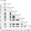 |
Fig. C.1. MOSFiT corner plot for the 56Ni decay fit. |
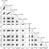 |
Fig. C.2. MOSFiT corner plot for the magnetar spindown fit. |
 |
Fig. C.3. MOSFiT corner plot for the CSI fit when s = 0. |
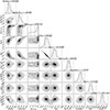 |
Fig. C.4. MOSFiT corner plot for the CSI fit when s = 2. |
 |
Fig. C.5. MOSFiT corner plot for the fallback fit. |
All Tables
Free and fixed parameters used in each MOSFiT model fit to the second peak, with prior distributions indicated.
Median posterior values and uncertainties of free parameters in each MOSFiT model fit and the score of each model.
Photometry of the host galaxy of SN 2023gpw based on publicly available pre-explosion data and our UVOT measurements.
All Figures
|
Fig. 1. Three-color NOT/ALFOSC images (blue: g; green: r; red: i) of SN 2023gpw a week before the light curve peak (left) and its faint host galaxy, visible at 189 d after the peak and with little contribution from the SN (right). The position of the SN in the galaxy is indicated, and the vertical bar corresponds to 10 arcseconds. |
| In the text | |
|
Fig. 2. Light curve of SN 2023gpw. The zero epoch corresponds to the g-band peak on MJD = 60085.0. Triangles denote 3σ upper limits, and shaded regions denote 1σ uncertainties of our GP fits. Epochs of spectra are marked with black (SEDM), gray (our other spectra) or blue (Kravtsov et al. 2023) lines, and the epoch of polarimetry is marked with a red line. Dashed lines show the evolution if the pre-gap decline rates had stayed constant during the gap, showing that the decline must have steepened some time after the last detection in the r and i bands. |
| In the text | |
|
Fig. 3. Top panel: Absolute g-band light curve of SN 2023gpw (black) compared to other SLSNe II. We include the SLSNe II presented by Kangas et al. (2022) (gray), the prototypical SN 2008es (purple; Gezari et al. 2009; Miller et al. 2009), CSS121015 (Benetti et al. 2014), and the two SLSNe II presented by Inserra et al. (2018) (SN 2013hx in teal and PS15br in red). Bottom panel: Same but in the r-band. A pronounced steepening in the r-band light curve, such as that in SN 2023gpw at some point before ∼ + 200 d, is not observed in other SLSNe II, though it is not excluded in some objects whose light curves do not continue this long. In both panels, the zero epoch corresponds to the g-band peak. |
| In the text | |
|
Fig. 4. Top panel: Optical colors of SN 2023gpw interpolated using a GP fit (shaded regions denote the 1σ uncertainty of this fit). The g − r color seems to become bluer during the rise to the peak, but the uncertainties of the measured colors are also consistent with no evolution in g − r until around the peak. Bottom panel: Comparison of the g − r color of SN 2023gpw with other SLSNe II (Miller et al. 2009; Inserra et al. 2018; Kangas et al. 2022), all corrected for Galactic extinction. The colors of comparison SNe have been GP-interpolated for visual clarity. |
| In the text | |
|
Fig. 5. SuperBol (Nicholl 2018) pseudo-bolometric light curve of SN 2023gpw. The values shown are based on either the full NUV-optical range (solid points) or only two or three bands and constant-color-based extrapolation of other bands (open points). |
| In the text | |
|
Fig. 6. Our moderate-resolution spectra of SN 2023gpw. Savitzky-Golay smoothing has been applied, and the +12-d spectrum has been binned by a factor of five. The original spectra are plotted in gray. The zero epoch corresponds to the g-band peak on MJD = 60085.0. Telluric absorption is marked with the ⨁ symbol and vertical dotted lines. The +278-day spectrum has no clear SN lines; only narrow emission lines from the host galaxy can be seen. Extinction correction has not been applied. The public PESSTO spectrum at +15 d does not include telluric-line correction. |
| In the text | |
|
Fig. 7. Low-resolution SEDM spectra of SN 2023gpw. The zero epoch corresponds to the g-band peak on MJD = 60085.0. Telluric absorption lines (⨁) are marked in vertical dotted lines. The marked lines are based on the higher-resolution spectra; the Ca II lines do not seem to match observed features here. |
| In the text | |
|
Fig. 8. Evolution of the Hα (black) and He IIλ4686 (red) line profiles in SN 2023gpw with the continuum subtracted on both sides. Telluric lines around Hα (⨁) are marked with dotted lines and the zero velocity with a dashed line. A weakening narrow component can be seen in the profile, while the wings of the broad component are disturbed by the telluric lines, but extend to several thousand km s−1 on both sides. |
| In the text | |
|
Fig. 9. Spectral evolution of SN 2023gpw (black) compared to the prototypical SN 2008es (red). Savitzky-Golay smoothing has been applied; the original spectra are plotted in gray. The zero epoch corresponds to the g-band peak. |
| In the text | |
|
Fig. 10. Spectral evolution of SN 2023gpw (black) compared to SLSNe II that resemble normal SNe II more than they do SN 2008es (Kangas et al. 2022). Savitzky-Golay smoothing has been applied; the original spectra are plotted in gray. The zero epoch corresponds to the g-band peak. |
| In the text | |
|
Fig. 11. Intensity-normalized Stokes q and u parameters of our polarimetry in the V and R bands on MJD = 60081.0, corresponding to −3.7 d. The filled circle corresponds to our best ISP estimate (see text) and the dashed circles to 0.5% and 1.0% polarization. The two bands are consistent with each other within 1σ and higher than the ISP. |
| In the text | |
|
Fig. 12. Blackbody fits (lines) to the observed SEDs of SN 2023gpw (points). An excess over the blackbody function appears and gradually strengthens after the peak. The W2 and M2 bands have been ignored in the fits denoted with dashed lines; the W1-band is roughly compatible with the optical data throughout the evolution. |
| In the text | |
|
Fig. 13. Evolution of the blackbody temperature (red) and radius (black) of SN 2023gpw. The empty symbols are based on less reliable fits using only the gr(i)-band data. The yellow line corresponds to the best-fit expansion velocity using the solid points only; this line reaches zero radius at −29 d, which is close to the first observed epoch at −31 d. |
| In the text | |
|
Fig. 14. MOSFiT light curve fits to SN 2023gpw using the different models described in the text. Late-time upper limits are represented as points, and the 3σ uncertainty corresponds to the measured limit. All models, but especially magnetar and fallback, have trouble reproducing the drop in brightness during the gap. The best fit by eye and score is the CSM model with s = 0. |
| In the text | |
|
Fig. 15. Spectral energy distribution of the host galaxy of SN 2023gpw from 1000 to 60 000 Å(black points) and the best-fitting Prospector model (solid line). The red squares represent the model-predicted magnitudes; some deviation can be seen in the NUV. The fitting parameters are shown in the upper-left corner. The abbreviation “n.o.f.” stands for the number of filters. |
| In the text | |
|
Fig. C.1. MOSFiT corner plot for the 56Ni decay fit. |
| In the text | |
|
Fig. C.2. MOSFiT corner plot for the magnetar spindown fit. |
| In the text | |
|
Fig. C.3. MOSFiT corner plot for the CSI fit when s = 0. |
| In the text | |
|
Fig. C.4. MOSFiT corner plot for the CSI fit when s = 2. |
| In the text | |
|
Fig. C.5. MOSFiT corner plot for the fallback fit. |
| In the text | |
Current usage metrics show cumulative count of Article Views (full-text article views including HTML views, PDF and ePub downloads, according to the available data) and Abstracts Views on Vision4Press platform.
Data correspond to usage on the plateform after 2015. The current usage metrics is available 48-96 hours after online publication and is updated daily on week days.
Initial download of the metrics may take a while.