| Issue |
A&A
Volume 705, January 2026
|
|
|---|---|---|
| Article Number | A236 | |
| Number of page(s) | 16 | |
| Section | Extragalactic astronomy | |
| DOI | https://doi.org/10.1051/0004-6361/202555974 | |
| Published online | 21 January 2026 | |
Evolution and mass dependence of UV-to-near-IR color gradients up to z = 2.5 from the Hubble Space Telescope and the James Webb Space Telescope
1
Sterrenkundig Observatorium, Universiteit Gent Krijgslaan 281 S9 9000 Gent, Belgium
2
Department of Astronomy, University of Michigan 1085 South University Avenue Ann Arbor MI 48109–1107, USA
3
Cosmic Dawn Center (DAWN), Niels Bohr Institute, University of Copenhagen Jagtvej 128 København N DK-2200, Denmark
4
STAR Institute, Université de Liège, Quartier Agora Allée du Six Aout 19c B-4000 Liege, Belgium
5
Department of Astronomy, University of Massachusetts Amherst MA 01003, USA
6
Department of Physics, University of Bath, Claverton Down Bath BA2 7AY, UK
★ Corresponding author: This email address is being protected from spambots. You need JavaScript enabled to view it.
Received:
16
June
2025
Accepted:
28
November
2025
Abstract
Aims. We present the redshift evolution of radial color gradients (in rest-frame U − V and V − J) for galaxies in the range 0.5 < z < 2.5 and investigate their origin and the dependence on stellar mass.
Methods. We selected ≈10 200 galaxies with stellar masses M★ > 109.5 M⊙ from publicly available JWST/NIRCam-selected catalogs. Using 2D Sérsic profile fits to account for point spread function broadening, we performed a spatially resolved spectral energy distribution fitting on HST and JWST/NIRCam photometry to retrieve accurate rest-frame U − V and V − J color gradients within 2 Re, F444W.
Results. The generally negative V − J color gradients of star-forming galaxies strongly depend on mass and redshift. For massive star-forming galaxies (M★ > 1010.5 M⊙) at z > 1.5, the V − J colors are ≈0.5 mag redder within the effective radius than outside on average. At all redshifts and throughout the entire stellar mass range, the V − J gradients strongly correlate with global attenuation (AV), which suggests that they predominantly trace dust attenuation gradients. Edge-on galaxies are redder and have stronger gradients at all z, although the correlation weakens at higher z. The U − V and V − J color gradients in the quiescent galaxy population, in contrast, are weakly negative (from ≈ − 0.1 to ≈ − 0.2 mag) but significant, and they depend little or not at all on stellar mass, redshift, or axis ratio. The implication is that quiescent galaxies must be largely transparent, with low AV, and their color gradients are mostly attributable to stellar population gradients.
Key words: galaxies: evolution / galaxies: general / galaxies: photometry / galaxies: structure / submillimeter: galaxies
© The Authors 2026
 Open Access article, published by EDP Sciences, under the terms of the Creative Commons Attribution License (https://creativecommons.org/licenses/by/4.0), which permits unrestricted use, distribution, and reproduction in any medium, provided the original work is properly cited.
This article is published in open access under the Subscribe to Open model. This email address is being protected from spambots. You need JavaScript enabled to view it. to support open access publication.
1. Introduction
Galaxies in the local Universe show red centers and bluer outskirts (i.e., Lin et al. 2017; Ellison et al. 2018). This characteristic is attributed to gradients in the age and to the composition of stellar populations at different radii, as well as to attenuation by dust. These color gradients were investigated in detail since the early 1970s (Sandage 1972), and their characteristics were studied by many researchers over the years (Peletier et al. 1990; de Jong 1996; Guo et al. 2011; Szomoru et al. 2013; Wuyts et al. 2013; Liu et al. 2016, 2017; Suess et al. 2019a; Miller et al. 2023; van der Wel et al. 2024). The color gradient in nearby quiescent galaxies can primarily be attributed to a radial metallicity gradient (i.e., Wu et al. 2005; Tortora et al. 2010, 2011; Sánchez-Blázquez et al. 2014; Goddard et al. 2017; Lin et al. 2024), and an age gradient is also a possibility (La Barbera & de Carvalho 2009).
The color gradients in present-day star-forming galaxies arise from various factors (Bell & de Jong 2000). The inner parts have older and more metal-rich stellar populations (Bell & de Jong 2000; Zibetti & Gallazzi 2022), a lower star formation activity (Tacchella et al. 2016; Lin et al. 2017; Belfiore et al. 2017, 2018; Ellison et al. 2018; Lin et al. 2019), and higher attenuation levels (Greener et al. 2020). These factors are all physically correlated, but it is important to recall that the origin of color gradients can vary from one galaxy to the next: Whereas the bulge of M31 lacks ongoing star formation, other nearby spirals such as M51 and M101 have significant star formation throughout.
These results prompted an investigation into the emergence of these gradients emerged by studying galaxies at earlier times at higher redshift. The Hubble Space Telescope (HST) led the way to unveiling the rest-frame optical colors of galaxies up to redshift z ≈ 1 (see, e.g., Hinkley & Im 2001; Menanteau et al. 2001; McGrath et al. 2008) and showed that color gradients were also present in these galaxies when the Universe was ≈6 Gyr old. The limited rest-frame optical wavelength range of these initial observations makes it difficult to distinguish dust and stellar population gradients: Galaxies (or galaxy regions) can appear redder because of old and/or metal-rich stellar populations or due to an increased dust attenuation. Near-IR emission at wavelengths between 1 and 3 μm, on the other hand, is less affected by dust attenuation and therefore allows us to separate the effects of dust and stellar population gradients. Several authors (see e.g., Wuyts et al. 2012; Szomoru et al. 2013; Liu et al. 2016; Wang et al. 2017; Liu et al. 2017; Suess et al. 2020) reported strong negative color gradients in high-redshift galaxies, that is, the galaxy centers are redder than their outskirts. These gradients notably imply smaller half-light radii at longer wavelengths and also more compact stellar mass distributions than stellar light distributions (i.e., McGrath et al. 2008; Dutton et al. 2011; Guo et al. 2011; Wuyts et al. 2012; Szomoru et al. 2013; Mosleh et al. 2017, 2020; Suess et al. 2019b,a, 2020; Miller et al. 2023; van der Wel et al. 2024). The effect of dust on these trends has been difficult to confirm without a near-IR view, however, which cannot be obtained with HST above a redshift of z > 0.4.
The James Webb Space Telescope (JWST) Near Infrared Camera (NIRCam) instrument solved this issue. Its high angular resolution at near-IR wavelengths, comparable to that of HST in the optical, now allows us to investigate the rest-frame > 1 μm wavelength range for galaxies up to redshift ≈2.5, when the Universe was just ≈2.5 Gyr old. Early JWST results for a small sample of galaxies (54 star-forming galaxies with M★ > 1010 M⊙ and 1.7 < z < 2.3) showed that the color gradients of galaxies are strongly negative up to z = 2.3 (Miller et al. 2022). These early findings were supported by several other works (e.g., Suess et al. 2022; Cutler et al. 2024; Ito et al. 2024; Ormerod et al. 2024; Martorano et al. 2024; Clausen et al. 2025) that measured the sizes of high-z galaxies as a function of wavelength and reported that galaxies are systematically smaller in the near-IR than in the optical. This is consistent with the trends seen in the present-day Universe. The early indications are that at z ≈ 2, dust gradients are more prominent than stellar population gradients, which is consistent with the hypothesis of dust-obscured bulge growth at earlier cosmic times (Tadaki et al. 2017; Tacchella et al. 2018; Nelson et al. 2019; Tadaki et al. 2020). At high redshift, the most massive galaxies have the highest AV values (Price et al. 2014; Cullen et al. 2018; Lorenz et al. 2024; Nersesian et al. 2025; van der Wel et al. 2025), and their optical profiles are shallower than in the near-IR (Martorano et al. 2025). This suggests that central mass concentrations (bulges or forming bulges) are present, but are strongly attenuated (see also Benton et al. 2024).
Using the complementarity of HST and JWST observations, we extend the early JWST results to a significantly larger sample of galaxies (> 10 200) with redshifts between 0.5 and 2.5 to investigate the origin and evolution across cosmic time of the U − V and V − J color gradients. The two main goals are (1) to determine the color gradients as a function of mass and galaxy type (star-forming versus quiescent), and (2) to interpret the cause of the gradients and its evolution with cosmic time. The paper is structured as follows: We present in Section 2 an overview of the sample selection (Sect. 2.1), the construction of light profiles across wavelength (Sect. 2.2), and the measurement of resolved rest-frame U − V and V − J colors, and we give an overview of the global galaxy properties (Sect. 2.3). We present in Section 3 the results of this work: the color gradients (Sect. 3.1), their effect on the UVJ diagram (Sect. 3.2), and their relation with inclination as traced by the projected axis ratio (Sect. 3.3). Finally, in Section 4, we summarize our results and draw our conclusions. Throughout the paper, we assume a standard flat-ΛCDM cosmology with H0 = 70 km s−1 Mpc−1 and Ωm = 0.3, and we adopt the AB magnitude system (Oke & Gunn 1983).
2. Data
2.1. Initial sample selection
The parent sample was drawn from the Dawn JWST Archive (DJA) morphological catalog1. This catalog contains photometric and morphological measurements for over 400 000 galaxies in the five CANDELS (Grogin et al. 2011; Koekemoer et al. 2011) fields observed with JWST/NIRCam over a plethora of different observational programs, such as PRIMER (Dunlop et al. 2021), COSMOS-Web (Casey et al. 2023), JADES (Eisenstein et al. 2023), FRESCO (Oesch et al. 2023), PANORAMIC (Williams et al. 2025), JEMS (Williams et al. 2023), and CEERS (Finkelstein et al. 2017, 2023).
The redshifts and global physical parameters (M★, rest-frame colors, and AV, which are relevant for this paper) were taken from the DJA morphological catalog as is. These were estimated via Spectra Energy Distribution (SED) fitting running the code EAZY (Brammer et al. 2008) on 0.5″ aperture photometry for all the available HST/ACS, HST/WFC3, JWST/NIRCam, and JWST/MIRI filters corrected to the total fluxes. The high angular resolution and sensitivity of the four instruments on this wide wavelength range (from 0.4 μm to 21 μm, although JWST/MIRI photometry is available for just about half of the targets) make it possible to recover accurate redshift measurements as well as stellar-mass measurements. EAZY was run on the agn_blue_sfhz_132 template set, which consists of 13 templates from the code called Flexible Stellar Populations Synthesis (FSPS Conroy et al. 2009; Conroy & Gunn 2010), which was built with a Chabrier (2003) initial mass function (IMF) and a Kriek & Conroy (2013) dust attenuation law, a template derived from the NIRSpec spectrum of a z = 8.5 galaxy presented by Carnall et al. (2023), and a template generated to replicate the JWST/NIRSpec spectrum of a z = 4.5 source perhaps consistent with an obscured AGN torus (Killi et al. 2024). For all the details about the EAZY setup and the global photometry, we refer to Valentino et al. (2023).
From the parent sample, we selected galaxies with an EAZY stellar mass M★ ≥ 109.5 M⊙. The low-mass high-redshift galaxies selected via this mass threshold were brighter by at least 2 magnitudes than the detection limit of the catalog in each field, implying that our sample was complete in stellar mass across the redshift range we investigated (0.5 < z < 2.5). An overview of the filters we used throughout is presented in Table 1. We did not use JWST/MIRI imaging data because their spatial resolution is lower than that of HST and JWST/NIRCam. This limited our analysis to rest frame ≈1.3 μm at z = 2.5 and to ≈3 μm at z = 0.5. The mosaics of the COSMOS and UDS fields were split in half with an overlapping region. This led to some duplicate objects in the catalog. For these objects, we only retained the object farthest away from the mosaic edges.
Filters for the Sérsic profile fitting and for computing the rest-frame colors.
Our starting catalog included 14 780 galaxies. Figure 1 shows nine representative galaxies divided into three stellar-mass bins at three (increasingly higher) redshifts. For each galaxy, we present three cutouts in the filters closer to the rest-frame U, V, and J bands, alongside their combination into an RGB image following a Richardson-Lucy deconvolution.
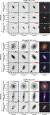 |
Fig. 1. Example of nine galaxies (field and DJA ID are shown left of each row) divided into three sets according to their stellar mass and ordered by redshift. For each galaxy, we present cutouts in the three filters that closely match the rest-frame U(blue)-V(green)-J(red) bands. The gray panels show the original images. To create the RGB images, each filter was first deconvolved with a Richardson-Lucy algorithm. We overplot ellipses with semimajor axis twice the effective radii measured in JWST/NIRCam F444W on the RBG image, as described in Sect. 2.2. |
In Figure 2 we present an overview of the properties of the star-forming galaxies in our sample, showing the evolution of AV with redshift in four stellar mass bins. We classified galaxies as star-forming or quiescent following Muzzin et al. (2013) based on UVJ colors. For star-forming galaxies with M★ < 1010.5 M⊙, AV depends little on redshift. Specifically, AV is ≈0.6 for M★ < 1010 M⊙ and ≈1.2 for 1010 < M★/M⊙ < 1010.5. More massive galaxies show a clear redshift evolution from median AV ≈ 1 at z ≈ 0.5 up to AV ≈ 3 at z ≈ 2.5. For a more detailed examination of the evolution of the colors and dust attenuation, we refer to van der Wel et al. (2025).
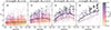 |
Fig. 2. Attenuation in the V band (AV) as a function of redshift in four stellar mass bins for star-forming galaxies color-coded with their V − J color. The white squares show the median in stellar mass bins, and the error bars show the statistical uncertainty ( |

The existence of a population of dusty galaxies at z ≳ 2 has been known for decades from near-IR surveys (Franx et al. 2003; Daddi et al. 2004; Labbé et al. 2005; Wuyts et al. 2007), far-infrared surveys (e.g., Shirley et al. 2019), and surveys at millimeter wavelengths (e.g., Smail et al. 1997, 2002; Chapman et al. 2003; Daddi et al. 2007). To provide this context, we cross-matched our catalog with the A3COSMOS and A3GOODSS catalogs (Adscheid et al. 2024), which contain all galaxies identified by ALMA during all the programs that surveyed the COSMOS and GOODS-S fields. We found a match for 92 submillimeter galaxies with a separation below 0.4″ (these are indicated by diamond markers throughout the work). These submillimeter galaxies are mostly seen at z > 1.5 and tend to be more massive than M★ > 1010.5 M⊙. All are characterized by the reddest V − J colors and have a median AV ≈ 3. According to their UVJ colors and to the definition of quiescence adopted throughout this work (Muzzin et al. 2013), all these 92 galaxies are classified as star-forming. This submillimeter-detected sample is not complete or representative for our sample; it is included to highlight the link between highly attenuated galaxies and dust-emission-selected samples, as also done by van der Wel et al. (2025).
2.2. Sérsic profile fits
To quantify color gradients, we used multiwavelength Sérsic profile fits. While these are crude summary descriptions of the light distribution, they address two important problems. First, the profile fits account for the wavelength-dependent PSF effects, which flatten the color gradients, as seen directly in the images (see, e.g., Fig. 1). Second, pixel-to-pixel variance is averaged out. To fairly compare color gradients between galaxies with a large variety of sizes and redshifts, we measured the colors and gradients in apertures relative to the half-light radius using photometry based on the galaxy 2D brightness model approximated with a single Sérsic profile. We thus performed a Sérsic profile fitting of all the galaxies using the code GALFITM (Häußler et al. 2013; Vika et al. 2013), a further developed version of GALFIT (Peng et al. 2002, 2010). The setup was the same overall as presented by Martorano et al. (2024) with minor differences.
Briefly, we created a segmentation map using the code SEP (Bertin & Arnouts 1996; Barbary 2016) for each field, and as the detection image, we used a stack of all available long-wavelength JWST/NIRCam filters (see Table 1 for the complete list of filters). We set a detection threshold at 3σ, a minimum area of 5 pixels, and a contrast ratio for object deblending of 0.02. For each source in the parent sample, we created cutouts that were large enough to contain 25 times more pixels for the background estimation than pixels falling in a segment. We set a minimum size of the cutout of 8″ and a maximum of 20″. Following Martorano et al. (2023), we simultaneously fit all objects identified in the segmentation map that were brighter (or up to one magnitude fainter) than the target together with the main source. This ensured that the light of bright objects in the cutouts was properly subtracted, and it thus allowed us to estimate the background better. Any other source in the cutout was masked with the corresponding segment of the segmentation map. The background was left as a free parameter in the fit performed by GALFITM. For each galaxy, we provided GALFITM with initial estimates for the position, magnitude, effective radius, and axis ratio based on the results obtained from the SEP analysis, and the initial guess for the position angle was set to 0 and for the Sérsic index to 2.3.
For each filter, we retrieved a point spread function (PSF) using the same procedure as outlined by Martorano et al. (2024). We selected a sample of candidate stars from the size-brightness relation in the filter F444W and observed in all the available filters; we masked all sources within 3″ and rejected candidate stars with nearby bright objects that might bias the background. From this set of objects, we visually selected the most suitable stellar candidates: isolated, bright, but not saturated in the center. The selected stars were stacked after normalizing their 0.3″ aperture flux and background subtraction. For JWST/NIRCam, we matched the flux of the stacked PSF in an annulus between 2.5″ and 3″ to the flux in the same annulus of the model PSF computed with WEBBPSF (Perrin et al. 2014). This guaranteed that any low-level residual background in the stacked PSF was removed. The PSFs we obtained were used as input for GALFITM.
Throughout this work, we assumed as the reference filter F444W. We discarded all galaxies whose fit in this filter failed or did not reach convergence for one of the parameters (≈4% of the whole sample). M.M. visually inspected the fit results for all the galaxies and flagged and removed evident mergers, gravitational lenses, and those for which the flux of bright sources near the target strongly polluted the photometry of the target itself. In addition, objects defined as segments, including multiple bright peaks, were removed. Finally, 22 galaxies were removed whose Sérsic index value in F444W hit the fit boundaries of 0.2−10. In total, another 5% of the sample were thus rejected, which left 13 332 galaxies for which useful color gradients were measured. The rejected targets are evenly distributed in stellar mass and redshift. Their removal therefore did not severely bias our sample.
For each galaxy, we computed the rest-frame 0.5 μm and 1.5 μm effective radii (Re, 0.5 μm and Re, 1.5 μm, respectively) by fitting a second-order Chebyshev polynomial to all the effective radii calculated in the filters investigated as a function of wavelength. We iterated this procedure 1000 times and Gaussian-sampled the Re measurements from their uncertainty distributions. The best polynomial was made of the median of the retrieved coefficients. This procedure was repeated to compute the Sérsic index at rest frame 0.5 μm (n0.5 μm) and 1.5 μm (n1.5 μm).
2.3. U − V and V − J rest-frame color gradients
Using the parameters recovered from the Sérsic profile fitting presented in Section 2.2, we constructed images of the intrinsic Sérsic profile (not PSF-convolved) in each filter. We measured fluxes within an ellipse whose center, semimajor axis, position angle, and axis ratio were taken from the F444W Sérsic profile fit. Likewise, we measured aperture photometry in an elliptical annulus between 1 and 2 Re, F444W3. We did not add flux residuals, as was done, for example, by Szomoru et al. (2010) and Suess et al. (2019a), to account for imperfections in the single Sérsic profile fits. The benefits of this approach do not, for our purposes, outweigh the additional uncertainties (noise). To verify that this was the case, we measured the residual F150W−F115W and F356W−F150W colors in the two apertures and their effect on the measured color gradient from the Sérsic profiles. These filters cover the rest-frame U, V, and J at z ≈ 2. The average change in the colors (and gradients) is < 1%, and the scatter is just 3%, which implies that the simplified description of the light profiles with single Sérsic profiles does not lead to relevant systematic effects in the measured color gradients (see Appendix A).
We used EAZY to derive rest-frame U, V and J fluxes by fitting the SED of both apertures, fixing the redshift at the value from the DJA catalog, and also adopting the same setup and zeropoints as were used for the DJA catalog to ensure that this did not induce systematic biases when we compared rest-frame fluxes we retrieved with those in the parent catalog. We defined the color gradient as the color difference between the outer (1 − 2 Re, F444W) and inner (< Re, F444W) apertures and adopted the convention that a galaxy with a red center and blue outskirts has a negative color gradient.
The use of deconvolved Sérsic profile models for the aperture photometry corrects for PSF effects that flatten gradients in the original PSF-convolved images, especially for small galaxies. The drawback of this method is the reliance on the single-component Sérsic models and the quality of the fits.
To avoid the effects of template mismatch, we required that for each of the rest-frame U, V, J bands an overlap of at least 50% with at least one of the HST or JWST filters listed in Table 1. In this way, the calculated rest-frame colors minimize interpolation by approximating the rest-frame colors to observed ones, without strong template dependences. About 22% of the galaxies were rejected by this constraint. The rejected galaxies are roughly uniformly distributed in redshift due to the field-to-field variation in filter sets, with the clear exception of lacking rest-frame J-band coverage at 0.88 < z < 0.90 due to the large gap between F200W and F277W. We note that the rejected 22% do not strongly affect the median trends in the results below, but they would have caused an increase in scatter due to the larger uncertainties induced by the interpolation between filters by EAZY.
The final sample contained 10 359 galaxies, 9444 of which are star-forming and 915 are quiescent. Out of the original 92 submillimeter-selected galaxies, 71 passed the selection.
3. Results
The superb angular resolution of JWST in the rest-frame near-IR and extensive wavelength coverage provided by the synergy of HST and JWST allowed us to probe beyond the global colors of galaxies and show the color gradients within them. Figure 1 already demonstrates visually striking color gradients in a small sample of galaxies. The galaxies in the figure are representative of three stellar mass bins and three redshift bins. While low-mass galaxies show similar colors and mild color gradients at any redshift, for M★ > 1010.5 M⊙, galaxies at z > 2 are systematically redder than at z < 1 and the cores are also redder than the outskirts. For the same set of nine galaxies shown in Figure 1, we present in Figure 3 the U − V and V − J color gradients that show the variation in the colors up to 2 Re, F444W in the UVJ plane. We also plot a grid of expected UVJ colors as a function of stellar metallicity and ages using the BPASS stellar libraries v.2.3.1 with solar [α/Fe] (Byrne et al. 2022) together with the AV vector that represents the effect of a simple dust screen as modeled within the THEMIS modeling framework (Jones et al. 2017). The low-mass galaxies show just mild color gradients at any redshift, while for higher stellar masses, the color gradients are systematically stronger, and U − V and V − J change by up to 1 mag between the core and the outskirts of the galaxy. The colors and color gradients for low-mass galaxies appear to be compatible with a combination of age and metallicity gradients, but at higher stellar masses, dust (possibly with nonstandard geometries) is clearly required to redden the templates. To support the qualitative color gradient trends shown in this figure, we quantify the variation in the color gradients with global galaxy properties and redshift in the next sections.
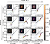 |
Fig. 3. UVJ plots for the same galaxies as in Figure 1. Each panel shows the UVJ color gradients in elliptical apertures with a width of 0.04″ up to an aperture of twice the effective radius in the filter F444W. The dashed black lines identify the quiescent region as defined by Muzzin et al. (2013). The white star with black contours shows the UVJ colors of the galaxy as in the DJA catalog, and the magenta (green) squares show the color measured within Re (1 − 2 Re). In the bottom right corner, we report the field and ID of the galaxy, together with its redshift, stellar mass, and global Av. In each panel, we show a metallicity and age grid from the BPASS stellar libraries, together with the theoretical AV vector induced by a dust screen. This figure shows different types of color gradients for the galaxies in the sample. |
3.1. Color gradients
In Figures 4 and 5, we present the U − V and V − J color gradients (hereafter Δ(U − V) and Δ(V − J)) of star-forming and quiescent galaxies as a function of redshift and in four different stellar mass bins. In the lower part of each panel, we show the median uncertainty on the color gradients (Appendix B). The solid black lines show the running median computed with the COBS library (Ng & Maechler 2007, 2022), which allows for a smoothed combination of a spline regression and quantile regression, highlighting nonlinear trends.
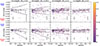 |
Fig. 4. Color gradients as a function of redshift for quiescent galaxies in four stellar mass bins and color-coded with global AV. The top row shows the U − V color gradients (Δ(U − V) = (U − V)1 < r/Re < 2 − (U − V)r < Re), and the bottom row shows the V − J color gradients (Δ(V − J) = (V − J)1 < r/Re < 2 − (V − J)r < Re). The black error bars in the lower left (right) corner of each panel show the median uncertainty on the color gradients for all the galaxies in that stellar mass bin with z < 1.5 (z > 1.5). The solid black lines show the running median, and the dashed lines show the 16−84 percentile range. The squares show the median color in redshift bins with a width of 0.25, and the (generally negligible) error bars represent the statistical uncertainty |

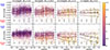 |
Fig. 5. Same as Fig. 4, but for star-forming galaxies. The diamonds identify submillimeter-selected galaxies. The black error bars in the lower part of each panel show the median uncertainty on the color gradients at that redshift. Δ(U − V) show no discernible redshift dependence and low-mass galaxies show no U − V gradients at z > 1.5. Conversely, Δ(V − J) shows a strong mass and redshift dependence. |
Figure 4 shows that quiescent galaxies display mild U − V gradients on average, with Δ(U − V)≈ − 0.1 mag, independent of redshift and mass. Their median Δ(V − J), in contrast, mildly depends on redshift: The gradients of galaxies at z > 2 and M★ < 1010.5 M⊙ are stronger than those of their lower-redshift counterpart, whereas this redshift evolution weakens and disappears at higher stellar mass (Spearman coefficients for M★ < 1010.5 M⊙ρ = −0.26, and for M★ > 1010.5 M⊙ρ = −0.06). As highlighted by the dashed lines showing the 16−84 percentiles, the scatter in the color gradients of low-mass galaxies strongly increases with redshift. This increased scatter is mostly due to the larger uncertainties in the color gradients (as shown by the systematically larger error bars in the bottom right corner), and has small number statistics. We visually inspected galaxies with gradients stronger than the 16th percentile (outliers) and found that in most cases, the gradients are highly uncertain, with a small subset of objects with genuinely strong gradients. Conversely, for massive quiescent galaxies, the uncertainty in the color gradients depends only mildly on redshift. This reflects the relative ease of measurement in larger objects (see, e.g., Martorano et al. 2024) and the absence of pronounced galaxy-to-galaxy variations. The low number of low-mass quiescent galaxies at high redshift, combined with the larger uncertainties in their color gradients, reduces our confidence in claiming a physical trend with redshift for these objects despite the values retrieved for the Spearman coefficient. The global AV of quiescent galaxies also varies mildly with redshift and increases to AV ≈ 1 (van der Wel et al. 2025), as expected from their higher sSFR at high-z (e.g., Leja et al. 2022). The AV estimates of these systems might be questionable, however, given the systematic uncertainties related to our limited knowledge of the intrinsic near-IR colors of evolved stellar populations. Nevertheless, the color gradients in quiescent galaxies primarily appear to originate with gradients in their stellar population (as also suggested by the BPASS comparison in Figure 3) and not by strong dust gradients (see also e.g., Suess et al. 2020).
The conclusions change for star-forming galaxies (Fig. 5). These are characterized by generally negative Δ(U − V), except at the low-mass end (M★ < 1010 M⊙), where star-forming galaxies show no U − V gradients at z > 1.5, with the scatter dominated (as for quiescent galaxies) by random uncertainties due to the limited sensitivity in the rest-frame U band. Higher-mass galaxies have slightly stronger Δ(U − V), but do not or only weakly depend on redshift. We found that Δ(U − V) is uncorrelated with global AV (Spearman rank correlation coefficient ≈0.1). The Δ(U − V) gradients are broadly comparable with the HST-based U − V gradients presented by Wuyts & Förster Schreiber (2020) despite the different method and photometry (they investigated color gradients by measuring Δ(U − V) in apertures smaller and larger than 2 kpc).
The V − J gradient Δ(V − J) varies more strongly than Δ(U − V) and also has stronger and more interesting trends with stellar mass and redshift. The uncertainties are small, even at large z, because of the exquisite depth of the NIRCam imaging. The gradients are significantly negative in general, even for low-mass galaxies (see also Miller et al. 2023, where g − r gradients are investigated). There is a strong mass-dependence and a strong redshift dependence for higher-mass galaxies (M★ > 1010.5 M⊙): The median and scatter are very large at z > 1.5. Δ(V − J) correlates strongly with global AV (Spearman rank correlation coefficient of ≈ − 0.6). The emergence of large fractions of high-AV galaxies at z > 1.5 discussed above goes hand in hand with the emergence of strong V − J color gradients. Among galaxies with AV > 2, gradients of Δ(V − J)≈ − 1 mag are not uncommon. These galaxies are one magnitude redder within their effective radius than outside. The large variation among massive star-forming galaxies at high redshift is not (entirely) due to uncertainties, but reflects a true galaxy-to-galaxy difference in dust properties and viewing angle. This is further addressed in Section 3.3. For reference, the population of 71 submillimeter-selected galaxies in our sample have a median  , and
, and  mag and
  mag, which is comparable to the general population of high-AV star-forming galaxies and suggests a link between IR-bright galaxies and centrally concentrated dust distributions.
In contrast to present-day massive galaxies, in which color gradients are driven by a combination of star formation, age, and metallicity gradients (Tortora et al. 2010, 2011; La Barbera & de Carvalho 2009), our results imply that for M★ > 1010.5 M⊙, the main driver of the color gradients in z > 1 galaxies is attenuation by dust. Several authors used other colors (i.e., Liu et al. 2016, 2017; Nelson et al. 2016; Wang et al. 2017) or methods (Miller et al. 2022, 2023; van der Wel et al. 2024; Martorano et al. 2024) and reached the same conclusion. Strong color gradients, together with a characteristically high AV in massive star-forming galaxies at z > 1, imply that these galaxies are building (or have already built) a core through intensive attenuated star formation that is unveiled when seen in the near-IR (Nelson et al. 2016, 2019; Miller et al. 2022; Le Bail et al. 2024; Benton et al. 2024; Tan et al. 2024; Nedkova et al. 2024; Martorano et al. 2025; Maheson et al. 2025). Evidence for bulge building in heavily dust obscured galaxy cores at z ≈ 2 has also been revealed using high-resolution ALMA 870 μm imaging (e.g., Hodge et al. 2016; Tadaki et al. 2017, 2020). In Appendix C we compare the color gradients we computed with the corresponding size ratio at different wavelengths. While these quantities both arise from changes in the light profile with wavelength, they are not identical.
3.2. Color gradients in the UVJ diagram
The color gradients presented in Section 3.1 have a strong effect on the UVJ diagram, which is frequently used (as in this paper) to separate star-forming and quiescent galaxies. In Figure 6 we present the UVJ diagram using the rest-frame U − V and V − J colors within the effective radius, computed from elliptical aperture photometry with a semimajor axis equal to Re, F444W.
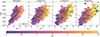 |
Fig. 6. UVJ diagram of the colors measured within the F444W effective radius, with hexbins containing at least five galaxies color-coded with the median global AV. The length and direction of the arrows indicate the median color shift from within the effective radius to the aperture between 1 Re and 2 Re, following our definition of a color gradient throughout this paper. A minimum of ten galaxies in the hexbin was required for drawing an arrow. The green diamonds highlight the U − V and V − J colors within 1 Re for the submillimeter-selected sample. |
Similarly to global colors (see Figure 2 and van der Wel et al. 2025), the central colors computed within 1 Re strongly correlate with the global AV, and highly attenuated galaxies show the reddest U − V and V − J colors. A significant population of galaxies with very red centers (V − J ≈ 3) again emerges at z > 1, but without a noticeable reddening in U − V. The color gradients, indicated by the black arrows in Figure 6, move the colors toward the bottom left corner of the UVJ plane, as expected for attenuation. Galaxies with the bluest central U − V colors (bottom left corner of each panel) show positive Δ(U − V) and mild or absent Δ(V − J), suggesting that they are undergoing a central starburst. Conversely, star-forming galaxies with V − J < 1 mag and U − V > 0.6 mag show Δ(U − V) < 0 and Δ(V − J)≈0, perhaps a sign of inside-out quenching (Tacchella et al. 2016) or of post-starburst systems (e.g., Belli et al. 2019).
As shown in Figures 4 and 5, quiescent galaxies are characterized by relatively mild color gradients. For z < 1 (leftmost panel of Fig. 6), there are as many galaxies with quiescent centers and star-forming outskirts as vice versa (≈35% of the quiescent population with z < 1), and their median gradients are very small, which places the centers and outskirts within or near the quiescent boundary. Conversely, for z > 1, there are about three times more galaxies with star-forming centers and quiescent outskirts than the other way around. Those with star-forming center have relatively weak  mag, but strong
  mag (e.g., almost horizontal arrows in Fig. 6). The colors are too red to be explained by metallicity gradients, but instead require a gray attenuation curve in the UV-optical, which is indeed seen for more attenuated galaxies (Salim et al. 2018; Barišić et al. 2020). The high AV value of galaxies with nearly horizontal gradient arrows in Fig. 6 suggests that dust gradients are the likely explanation for the color gradients. Under this assumption, these galaxies have obscured star-forming cores and quiescent little attenuated outskirts. In the small subset of galaxies with quiescent cores and star-forming outskirts, the pattern is consistent with that observed in some present-day massive galaxies such as M31. They exhibit strong
  mag, but weak
  mag (see e.g., Fig. 3 top left panel). This might imply a genuine population gradient (i.e., Ellison et al. 2018, and references therein) as in M31, or at least a gradient in star formation activity that affects U − V more strongly than V − J (e.g., Gebek et al. 2025). Truly quiescent cores such as in M31 are relatively rare. Instead, it is more common to have star formation throughout, such as in local spiral galaxies like M51, M83, M101, and the Milky Way. The color gradients are generally caused by a combination of factors that vary from one galaxy to the next. Cosmological simulations are the ideal framework for properly identifying the factors that cause global colors and color gradients. They currently still cannot describe all the features in observed UVJ diagrams (Donnari et al. 2019; Akins et al. 2022; Gebek et al. 2025). Following Gebek et al., however, we might expect our results to imply a specialized dust geometry; those authors reported that obtaining large V − J colors without strongly affecting the distribution of U − V colors requires birthcloud-like attenuation around all stars younger than 1 Gyr.
The submillimeter-selected galaxies, which are among the most attenuated of all galaxies in our sample, almost all lie in the top right corner of the UVJ diagram and have similar color gradients to all other galaxies with AV > 3. The color gradients of only 4 out of the 71 submillimeter galaxies resemble a star-forming core and quiescent outskirts. Two of them show extended disks with spiral arms and indications of ongoing minor mergers. The other two show no morphological features.
3.3. Color gradients and axis ratios. Trends with inclination
The results presented in the previous sections indicate that in massive star-forming galaxies at z > 1.5, dust attenuation in the rest-frame V band is centrally concentrated within the galaxies. At lower z, the integrated (galaxy-averaged) AV values are lower and the gradients are weaker. To further explore the nature of this evolution with redshift, we considered the connection between the axis ratio as a proxy for the viewing angle and attenuation properties (as traced by colors and color gradients) for quiescent and star-forming galaxies with M★ > 1010.5 M⊙. The motivation for this mass selection was that these star-forming galaxies are most likely to be disk-like in a geometric sense (oblate and flattened van der Wel et al. 2014; Zhang et al. 2019) and as expressed by their kinematic properties (e.g., Förster Schreiber et al. 2009; Wisnioski et al. 2015).
For disks (flat oblates), the projected axis ratio q as measured in the F444W filter by the two-dimensional Sérsic light profile fit, is a good tracer of the inclination, that is, a one-dimensional viewing angle. In Figures 7 and 8, we show the distribution of q and the global U − V and V − J colors in redshift bins for the quiescent and star-forming population, respectively.
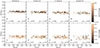 |
Fig. 7. Projected axis ratio (q) observed in JWST/NIRCam-F444W against U − V (upper panels) and V − J (lower panels) colors in four redshift bins. The color-coding shows the color gradient computed as the difference between the color between 1−2 Re and 0−1 Re. We only show quiescent galaxies with stellar mass M★ ≥ 1010.5 M⊙. In the lower left corner, we show the median uncertainties on the rest frame colors and axis ratios and the Spearman correlation coefficient between the axis ratio and the color, and in the right corner, we show that between the axis ratio and the color gradient. |
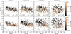 |
Fig. 8. Same as Figure 7, but for M★ ≥ 1010.5 M⊙ star-forming galaxies. The diamonds show submillimeter-selected galaxies. The correlation between the colors and q decreases with redshift. |
For the population of quiescent galaxies, little correlation between color and axis ratio q is expected (as suggested by their tight color sequences; see van der Wel et al. 2025, and as confirmed by the low Spearman correlation coefficients reported in the bottom left corner of each panel of Fig. 7). Many if not most of these galaxies are shaped like oblate disks (Chang et al. 2013) up to at least z = 2. The absence of a correlation with q then implies that color is independent of inclination, which we interpret as evidence for transparency, that is, low dust columns. This agrees with the recent result that even quiescent galaxies with significant molecular gas reservoirs do not have much dust (Spilker et al. 2025). Changing the definition of the quiescent boundary in the UVJ diagram adopted in this work (now set to V − J < 1.5; Muzzin et al. 2013) did not alter the conclusions drawn on the basis of Fig. 7. Further investigation of dust in quiescent galaxies requires a selection based on the sSFR (possibly retrieved from a nonparametric SED fitting including far-IR photometry) to avoid any color-selection systematics.
Conversely, for star-forming galaxies at z < 1.5, the trend is familiar and expected: Flat (edge-on) galaxies are redder than round (face-on) galaxies. The connection between color and viewing angle (well traced by the axis ratio for low-z star-forming galaxies; see e.g., van der Wel et al. 2014) was previously established at z ≈ 1 by Patel et al. (2012). The small scatter in color at fixed q (0.2 mag in V − J) is also noteworthy. The variation among the galaxies in terms of their intrinsic properties (star formation, stellar population, and dust content) must be relatively weak, and to a large extent, the observed colors are determined by inclination. The color gradient and axis ratio are correlated as well: Face-on galaxies (large q) have weaker gradients than edge-on (low q) galaxies (Spearman correlation coefficient ρ(U − V) ≈ −0.3 and ρ(V − J) ≈ −0.6). In edge-on galaxies, the dust obscures the central region more than the outer parts. This correlation is weaker than the q-color correlation, but still significant, especially for Δ(V − J) (in fact, ρΔ(U − V) ≈ 0.1 and ρΔ(V − J) ≈ 0.4). These trends together are consistent with the result that massive present-day spiral galaxies (with Vc > 120 km s−1; M★ ≳ 1010 M⊙) show thin, smooth, regular and galaxy-wide dust lanes that are aligned with the gravitationally dominant stellar disk (Dalcanton et al. 2004).
At z > 1.5, however, the trends change and the correlations between q and colors and color gradients weaken (with ρ(U − V), which drops to ≈ − 0.1 and ρ(V − J) to ≈ − 0.2). The viewing angle no longer matters in the same manner as at later cosmic times. To some extent, this is due to the less obviously disk-like nature of at least a subset of the galaxies. Rotational support decreases with redshift (Kassin et al. 2012; Wisnioski et al. 2015; Übler et al. 2019), and the geometry distribution is more varied (van der Wel et al. 2014; Zhang et al. 2019) so that the axis ratio no longer tracks the viewing angle in a unique manner. The disappearance of disks is not the full story, however. A large fraction of galaxies is still disk-like in nature, the evidence for which was recently bolstered by the large observed fraction of galaxies with spiral arms in this mass and redshift range (e.g., Espejo Salcedo et al. 2025 found 72% of the galaxies with 2 < z < 2.5 to be disk-like and 20% to host spiral arms). They can only exist in relatively thin stellar and/or gaseous disks.
The correlations between q and the color (gradient) information are still less obvious in statistical terms and less straightforward to interpret, however. At z > 2, the q − (V − J) correlation is still significant (ρ(V − J) = −0.22), but weaker than at z < 1.5, and with a very clear increase in scatter at fixed q (0.7 mag at z > 2 compared to 0.2 mag at z < 1). Likewise, the q − Δ(V − J) correlation persists at z > 2 (ρΔ(V − J) = 0.21), if slightly weaker, with stronger gradients for flat (edge-on) galaxies. For U − V, the picture is different from V − J.
At z > 2, there is no q − (U − V) correlation (ρ(U − V) ≈ 0), and, if anything, a weak anticorrelation between q and Δ(U − V) (ρΔ(U − V) = −0.15), with slightly stronger gradients in round (face-on) galaxies. This trend is driven by a population of galaxies with blue integrated U − V colors, weak U − V gradients, but red V − J colors and strong V − J gradients. This population is already apparent at 1 < z < 1.5, and a prototypical example is shown in the center of the 3 × 3 set of panels in Figure 3. The U − V trends are explained by a patchy but not clearly radially varying distribution of relatively unobscured star formation at the side of the underlying disk that is pointed in the direction of the observer.
Taken together, these color and color gradient trends with q clearly show that the dust-to-star geometry at z > 1.5 is fundamentally different from the thin regular dust-lane geometry seen at 0 < z < 1.5. The evidence suggests that the dust distribution still retains some of the axisymmetric characteristics of a dust lane, given the bluer colors of face-on galaxies. The much higher AV values also imply, however, that the dust lane must be more vertically extended and must look more like a patchy thick disk that obscures the majority of all intrinsic rest-frame V-band light. A thick disk of dust like this must also be centrally concentrated, as implied by the color gradients, which are stronger for edge-on high-AV galaxies (see the correlation coefficients in Figure 8). Finally, the dust distribution is also rougher and more regular than their thin present-day counterparts, as indicated by the large scatter in the U − V and V − J colors and their gradients. This dust model closely matches the model discussed in the rightmost panel of Fig. 7 of Gebek et al. (2025).
4. Conclusions
We used the combination of HST and JWST imaging to quantify and examine gradients in rest-frame U − V and V − J colors for over 10 200 galaxies at redshifts 0.5 < z < 2.5 with stellar masses M★ > 109.5 M⊙. To stabilize our color measurements against issues related to background subtraction and the PSF, we performed multiwavelength 2D brightness modeling that fits a Sérsic profile to each galaxy at each observed wavelength. We then measured the colors from these Sérsic profiles.
The U − V color gradients in star-forming galaxies (Fig. 5) depend mildly on stellar mass (with stronger gradients for more massive galaxies) and weakly on redshift evolution. Their V − J color gradients, on the other hand, depend strongly on mass and redshift, and high-mass 2 < z < 2.5 galaxies show the strongest gradients on average. The central regions, in particular, have much redder V − J colors than can be explained by any dust-free stellar population. In combination with the strong link between V − J gradient and global AV we found, this suggests that the optical and near-IR colors of high-mass galaxies reflect a strong attenuation gradient and highly obscured centers. Together with stellar population gradients, strong dust gradients produce U − V and V − J gradients that systematically shift the galaxy population within the UVJ color plane. Finally, the strongest gradients and reddest colors were seen for edge-on galaxies at z > 1.5. The high AV values imply a vertically extended dust geometry in the plane of the stellar disk and not the thin dust lanes seen at lower z.
The quiescent galaxy population, on the other hand, has negative radial gradients in both U − V and V − J colors, with little or no redshift evolution. The lack of a relation between viewing angle (inclination) and color implies that these galaxies are largely transparent and, in line with our knowledge of gradients in present-day early-type galaxies, that the color gradients are the result of stellar population gradients. The lack of a redshift evolution in the strength of the gradient might be the result of weakening age-induced gradients with cosmic time that are compensated for by increasing metallicity gradients. Further study is needed to confirm this picture, however. The results of this work serve as a benchmark for the examination of the origin of gradients in cosmological simulations (e.g., Donnari et al. 2019; Akins et al. 2022; Gebek et al. 2025) to help us understand the dust geometry and structure of galaxies 10 Gyr ago.
Acknowledgments
MM acknowledges the financial support of the Flemish Fund for Scientific Research (FWO-Vlaanderen), research project G030319N. (Some of) The data products presented herein were retrieved from the Dawn JWST Archive (DJA). DJA is an initiative of the Cosmic Dawn Center (DAWN), which is funded by the Danish National Research Foundation under grant DNRF140.
References
- Adscheid, S., Magnelli, B., Liu, D., et al. 2024, A&A, 685, A1 [NASA ADS] [CrossRef] [EDP Sciences] [Google Scholar]
- Akins, H. B., Narayanan, D., Whitaker, K. E., et al. 2022, ApJ, 929, 94 [NASA ADS] [CrossRef] [Google Scholar]
- Barbary, K. 2016, J. Open Source Softw., 1, 58 [Google Scholar]
- Barišić, I., Pacifici, C., van der Wel, A., et al. 2020, ApJ, 903, 146 [CrossRef] [Google Scholar]
- Belfiore, F., Maiolino, R., Maraston, C., et al. 2017, MNRAS, 466, 2570 [Google Scholar]
- Belfiore, F., Maiolino, R., Bundy, K., et al. 2018, MNRAS, 477, 3014 [Google Scholar]
- Bell, E. F., & de Jong, R. S. 2000, MNRAS, 312, 497 [NASA ADS] [CrossRef] [Google Scholar]
- Belli, S., Newman, A. B., & Ellis, R. S. 2019, ApJ, 874, 17 [Google Scholar]
- Benton, C. E., Nelson, E. J., Miller, T. B., et al. 2024, ApJ, 974, L28 [Google Scholar]
- Bertin, E., & Arnouts, S. 1996, A&AS, 117, 393 [NASA ADS] [CrossRef] [EDP Sciences] [Google Scholar]
- Brammer, G. B., van Dokkum, P. G., & Coppi, P. 2008, ApJ, 686, 1503 [Google Scholar]
- Brammer, G. B., Whitaker, K. E., van Dokkum, P. G., et al. 2011, ApJ, 739, 24 [NASA ADS] [CrossRef] [Google Scholar]
- Byrne, C. M., Stanway, E. R., Eldridge, J. J., McSwiney, L., & Townsend, O. T. 2022, MNRAS, 512, 5329 [NASA ADS] [CrossRef] [Google Scholar]
- Carnall, A. C., McLure, R. J., Dunlop, J. S., et al. 2023, Nature, 619, 716 [NASA ADS] [CrossRef] [Google Scholar]
- Casey, C. M., Kartaltepe, J. S., Drakos, N. E., et al. 2023, ApJ, 954, 31 [NASA ADS] [CrossRef] [Google Scholar]
- Chabrier, G. 2003, PASP, 115, 763 [Google Scholar]
- Chang, Y.-Y., van der Wel, A., Rix, H.-W., et al. 2013, ApJ, 773, 149 [NASA ADS] [CrossRef] [Google Scholar]
- Chapman, S. C., Windhorst, R., Odewahn, S., Yan, H., & Conselice, C. 2003, ApJ, 599, 92 [NASA ADS] [CrossRef] [Google Scholar]
- Clausen, M., Momcheva, I. G., Whitaker, K. E., et al. 2025, ApJ, 993, 106 [Google Scholar]
- Conroy, C., & Gunn, J. E. 2010, ApJ, 712, 833 [Google Scholar]
- Conroy, C., Gunn, J. E., & White, M. 2009, ApJ, 699, 486 [Google Scholar]
- Cullen, F., McLure, R. J., Khochfar, S., et al. 2018, MNRAS, 476, 3218 [Google Scholar]
- Cutler, S. E., Whitaker, K. E., Weaver, J. R., et al. 2024, ApJ, 967, L23 [NASA ADS] [CrossRef] [Google Scholar]
- Daddi, E., Cimatti, A., Renzini, A., et al. 2004, ApJ, 600, L127 [Google Scholar]
- Daddi, E., Dickinson, M., Morrison, G., et al. 2007, ApJ, 670, 156 [NASA ADS] [CrossRef] [Google Scholar]
- Dalcanton, J. J., Yoachim, P., & Bernstein, R. A. 2004, ApJ, 608, 189 [NASA ADS] [CrossRef] [Google Scholar]
- de Jong, R. S. 1996, A&A, 313, 45 [NASA ADS] [Google Scholar]
- Donnari, M., Pillepich, A., Nelson, D., et al. 2019, MNRAS, 485, 4817 [Google Scholar]
- Dunlop, J. S., Abraham, R. G., Ashby, M. L. N., et al. 2021, PRIMER: Public Release IMaging for Extragalactic Research, JWST Proposal. Cycle 1 [Google Scholar]
- Dutton, A. A., van den Bosch, F. C., Faber, S. M., et al. 2011, MNRAS, 410, 1660 [NASA ADS] [Google Scholar]
- Eisenstein, D. J., Willott, C., Alberts, S., et al. 2023, ArXiv e-prints [arXiv:2306.02465] [Google Scholar]
- Ellison, S. L., Sánchez, S. F., Ibarra-Medel, H., et al. 2018, MNRAS, 474, 2039 [Google Scholar]
- Espejo Salcedo, J. M., Pastras, S., Vácha, J., et al. 2025, A&A, 700, A42 [NASA ADS] [CrossRef] [EDP Sciences] [Google Scholar]
- Finkelstein, S. L., Dickinson, M., Ferguson, H. C., et al. 2017, The Cosmic Evolution Early Release Science (CEERS) Survey, JWST Proposal ID 1345. Cycle 0 Early Release Science [Google Scholar]
- Finkelstein, S. L., Bagley, M. B., Ferguson, H. C., et al. 2023, ApJ, 946, L13 [NASA ADS] [CrossRef] [Google Scholar]
- Förster Schreiber, N. M., Genzel, R., Bouché, N., et al. 2009, ApJ, 706, 1364 [Google Scholar]
- Franx, M., Labbé, I., Rudnick, G., et al. 2003, ApJ, 587, L79 [Google Scholar]
- Gebek, A., Diemer, B., Martorano, M., et al. 2025, A&A, 695, A90 [NASA ADS] [CrossRef] [EDP Sciences] [Google Scholar]
- Gillman, S., Smail, I., Gullberg, B., et al. 2024, A&A, 691, A299 [NASA ADS] [CrossRef] [EDP Sciences] [Google Scholar]
- Goddard, D., Thomas, D., Maraston, C., et al. 2017, MNRAS, 466, 4731 [NASA ADS] [Google Scholar]
- Greener, M. J., Aragón-Salamanca, A., Merrifield, M. R., et al. 2020, MNRAS, 495, 2305 [CrossRef] [Google Scholar]
- Grogin, N. A., Kocevski, D. D., Faber, S. M., et al. 2011, ApJS, 197, 35 [NASA ADS] [CrossRef] [Google Scholar]
- Guo, Y., Giavalisco, M., Cassata, P., et al. 2011, ApJ, 735, 18 [NASA ADS] [CrossRef] [Google Scholar]
- Häußler, B., Bamford, S. P., Vika, M., et al. 2013, MNRAS, 430, 330 [Google Scholar]
- Hinkley, S., & Im, M. 2001, ApJ, 560, L41 [Google Scholar]
- Hodge, J. A., Swinbank, A. M., Simpson, J. M., et al. 2016, ApJ, 833, 103 [Google Scholar]
- Ito, K., Valentino, F., Brammer, G., et al. 2024, ApJ, 964, 192 [CrossRef] [Google Scholar]
- Jones, A. P., Köhler, M., Ysard, N., Bocchio, M., & Verstraete, L. 2017, A&A, 602, A46 [NASA ADS] [CrossRef] [EDP Sciences] [Google Scholar]
- Kassin, S. A., Weiner, B. J., Faber, S. M., et al. 2012, ApJ, 758, 106 [NASA ADS] [CrossRef] [Google Scholar]
- Kelvin, L. S., Driver, S. P., Robotham, A. S. G., et al. 2012, MNRAS, 421, 1007 [Google Scholar]
- Kennedy, R., Bamford, S. P., Baldry, I., et al. 2015, MNRAS, 454, 806 [NASA ADS] [CrossRef] [Google Scholar]
- Killi, M., Watson, D., Brammer, G., et al. 2024, A&A, 691, A52 [NASA ADS] [CrossRef] [EDP Sciences] [Google Scholar]
- Koekemoer, A. M., Faber, S. M., Ferguson, H. C., et al. 2011, ApJS, 197, 36 [NASA ADS] [CrossRef] [Google Scholar]
- Kriek, M., & Conroy, C. 2013, ApJ, 775, L16 [NASA ADS] [CrossRef] [Google Scholar]
- La Barbera, F., & de Carvalho, R. R. 2009, ApJ, 699, L76 [Google Scholar]
- Labbé, I., Huang, J., Franx, M., et al. 2005, ApJ, 624, L81 [Google Scholar]
- Le Bail, A., Daddi, E., Elbaz, D., et al. 2024, A&A, 688, A53 [NASA ADS] [CrossRef] [EDP Sciences] [Google Scholar]
- Leja, J., Speagle, J. S., Ting, Y.-S., et al. 2022, ApJ, 936, 165 [NASA ADS] [CrossRef] [Google Scholar]
- Lin, L., Belfiore, F., Pan, H.-A., et al. 2017, ApJ, 851, 18 [Google Scholar]
- Lin, L., Hsieh, B.-C., Pan, H.-A., et al. 2019, ApJ, 872, 50 [Google Scholar]
- Lin, L., Shen, S., Yesuf, H. M., Mao, Y.-W., & Hao, L. 2024, ApJ, 977, 175 [Google Scholar]
- Liu, F. S., Jiang, D., Guo, Y., et al. 2016, ApJ, 822, L25 [NASA ADS] [CrossRef] [Google Scholar]
- Liu, F. S., Jiang, D., Faber, S. M., et al. 2017, ApJ, 844, L2 [Google Scholar]
- Lorenz, B., Kriek, M., Shapley, A. E., et al. 2024, ApJ, 975, 187 [NASA ADS] [CrossRef] [Google Scholar]
- Maheson, G., Tacchella, S., Belli, S., et al. 2025, ArXiv e-prints [arXiv:2504.15346] [Google Scholar]
- Martorano, M., van der Wel, A., Bell, E. F., et al. 2023, ApJ, 957, 46 [NASA ADS] [CrossRef] [Google Scholar]
- Martorano, M., van der Wel, A., Baes, M., et al. 2024, ApJ, 972, 134 [Google Scholar]
- Martorano, M., van der Wel, A., Baes, M., et al. 2025, A&A, 694, A76 [NASA ADS] [CrossRef] [EDP Sciences] [Google Scholar]
- McGrath, E. J., Stockton, A., Canalizo, G., Iye, M., & Maihara, T. 2008, ApJ, 682, 303 [Google Scholar]
- Menanteau, F., Abraham, R. G., & Ellis, R. S. 2001, MNRAS, 322, 1 [Google Scholar]
- Miller, T. B., Whitaker, K. E., Nelson, E. J., et al. 2022, ApJ, 941, L37 [NASA ADS] [CrossRef] [Google Scholar]
- Miller, T. B., van Dokkum, P., & Mowla, L. 2023, ApJ, 945, 155 [NASA ADS] [CrossRef] [Google Scholar]
- Mosleh, M., Tacchella, S., Renzini, A., et al. 2017, ApJ, 837, 2 [NASA ADS] [CrossRef] [Google Scholar]
- Mosleh, M., Hosseinnejad, S., Hosseini-ShahiSavandi, S. Z., & Tacchella, S. 2020, ApJ, 905, 170 [NASA ADS] [CrossRef] [Google Scholar]
- Muzzin, A., Marchesini, D., Stefanon, M., et al. 2013, ApJ, 777, 18 [NASA ADS] [CrossRef] [Google Scholar]
- Nedkova, K. V., Rafelski, M., Teplitz, H. I., et al. 2024, ApJ, 970, 188 [NASA ADS] [CrossRef] [Google Scholar]
- Nelson, E. J., van Dokkum, P. G., Momcheva, I. G., et al. 2016, ApJ, 817, L9 [CrossRef] [Google Scholar]
- Nelson, E. J., Tadaki, K.-I., Tacconi, L. J., et al. 2019, ApJ, 870, 130 [NASA ADS] [CrossRef] [Google Scholar]
- Nersesian, A., van der Wel, A., Gallazzi, A. R., et al. 2025, A&A, 695, A86 [NASA ADS] [CrossRef] [EDP Sciences] [Google Scholar]
- Ng, P., & Maechler, M. 2007, Stat. Model., 7, 315 [CrossRef] [Google Scholar]
- Ng, P., & Maechler, M. 2022, COBS– Constrained B-splines (Sparse matrix based), r package version 1.3-5 [Google Scholar]
- Oesch, P. A., Brammer, G., Naidu, R. P., et al. 2023, MNRAS, 525, 2864 [NASA ADS] [CrossRef] [Google Scholar]
- Oke, J. B., & Gunn, J. E. 1983, ApJ, 266, 713 [NASA ADS] [CrossRef] [Google Scholar]
- Ormerod, K., Conselice, C. J., Adams, N. J., et al. 2024, MNRAS, 527, 6110 [Google Scholar]
- Patel, S. G., Holden, B. P., Kelson, D. D., et al. 2012, ApJ, 748, L27 [NASA ADS] [CrossRef] [Google Scholar]
- Peletier, R. F., Davies, R. L., Illingworth, G. D., Davis, L. E., & Cawson, M. 1990, AJ, 100, 1091 [Google Scholar]
- Peng, C. Y., Ho, L. C., Impey, C. D., & Rix, H.-W. 2002, AJ, 124, 266 [Google Scholar]
- Peng, C. Y., Ho, L. C., Impey, C. D., & Rix, H.-W. 2010, AJ, 139, 2097 [Google Scholar]
- Perrin, M. D., Sivaramakrishnan, A., Lajoie, C.-P., et al. 2014, SPIE Conf. Ser., 9143, 91433X [NASA ADS] [Google Scholar]
- Price, S. H., Kriek, M., Brammer, G. B., et al. 2014, ApJ, 788, 86 [NASA ADS] [CrossRef] [Google Scholar]
- Price, S. H., Suess, K. A., Williams, C. C., et al. 2025, ApJ, 980, 11 [Google Scholar]
- Ren, J., Liu, F. S., Li, N., et al. 2025, ApJ, 982, 200 [Google Scholar]
- Salim, S., Boquien, M., & Lee, J. C. 2018, ApJ, 859, 11 [Google Scholar]
- Sánchez-Blázquez, P., Rosales-Ortega, F. F., Méndez-Abreu, J., et al. 2014, A&A, 570, A6 [NASA ADS] [CrossRef] [EDP Sciences] [Google Scholar]
- Sandage, A. 1972, ApJ, 176, 21 [CrossRef] [Google Scholar]
- Shirley, R., Roehlly, Y., Hurley, P. D., et al. 2019, MNRAS, 490, 634 [Google Scholar]
- Smail, I., Ivison, R. J., & Blain, A. W. 1997, ApJ, 490, L5 [NASA ADS] [CrossRef] [Google Scholar]
- Smail, I., Ivison, R. J., Blain, A. W., & Kneib, J. P. 2002, MNRAS, 331, 495 [CrossRef] [Google Scholar]
- Spilker, J. S., Whitaker, K. E., Narayanan, D., et al. 2025, ApJ, 993, L40 [Google Scholar]
- Suess, K. A., Kriek, M., Price, S. H., & Barro, G. 2019a, ApJ, 877, 103 [NASA ADS] [CrossRef] [Google Scholar]
- Suess, K. A., Kriek, M., Price, S. H., & Barro, G. 2019b, ApJ, 885, L22 [NASA ADS] [CrossRef] [Google Scholar]
- Suess, K. A., Kriek, M., Price, S. H., & Barro, G. 2020, ApJ, 899, L26 [Google Scholar]
- Suess, K. A., Bezanson, R., Nelson, E. J., et al. 2022, ApJ, 937, L33 [NASA ADS] [CrossRef] [Google Scholar]
- Szomoru, D., Franx, M., van Dokkum, P. G., et al. 2010, ApJ, 714, L244 [Google Scholar]
- Szomoru, D., Franx, M., van Dokkum, P. G., et al. 2013, ApJ, 763, 73 [NASA ADS] [CrossRef] [Google Scholar]
- Tacchella, S., Dekel, A., Carollo, C. M., et al. 2016, MNRAS, 458, 242 [NASA ADS] [CrossRef] [Google Scholar]
- Tacchella, S., Carollo, C. M., Förster Schreiber, N. M., et al. 2018, ApJ, 859, 56 [Google Scholar]
- Tadaki, K.-I., Genzel, R., Kodama, T., et al. 2017, ApJ, 834, 135 [NASA ADS] [CrossRef] [Google Scholar]
- Tadaki, K.-I., Belli, S., Burkert, A., et al. 2020, ApJ, 901, 74 [NASA ADS] [CrossRef] [Google Scholar]
- Tan, Q.-H., Daddi, E., Magnelli, B., et al. 2024, Nature, 636, 69 [Google Scholar]
- Tortora, C., Napolitano, N. R., Cardone, V. F., et al. 2010, MNRAS, 407, 144 [Google Scholar]
- Tortora, C., Napolitano, N. R., Romanowsky, A. J., et al. 2011, MNRAS, 418, 1557 [Google Scholar]
- Übler, H., Genzel, R., Wisnioski, E., et al. 2019, ApJ, 880, 48 [Google Scholar]
- Valentino, F., Brammer, G., Gould, K. M. L., et al. 2023, ApJ, 947, 20 [NASA ADS] [CrossRef] [Google Scholar]
- van der Wel, A., Chang, Y.-Y., Bell, E. F., et al. 2014, ApJ, 792, L6 [NASA ADS] [CrossRef] [Google Scholar]
- van der Wel, A., Martorano, M., Häußler, B., et al. 2024, ApJ, 960, 53 [NASA ADS] [CrossRef] [Google Scholar]
- van der Wel, A., Martorano, M., Marchesini, D., et al. 2025, A&A, 701, A30 [NASA ADS] [CrossRef] [EDP Sciences] [Google Scholar]
- Vika, M., Bamford, S. P., Häußler, B., et al. 2013, MNRAS, 435, 623 [NASA ADS] [CrossRef] [Google Scholar]
- Wang, W., Faber, S. M., Liu, F. S., et al. 2017, MNRAS, 469, 4063 [CrossRef] [Google Scholar]
- Williams, C. C., Tacchella, S., Maseda, M. V., et al. 2023, ApJS, 268, 64 [NASA ADS] [CrossRef] [Google Scholar]
- Williams, C. C., Oesch, P. A., Weibel, A., et al. 2025, ApJ, 979, 140 [Google Scholar]
- Wisnioski, E., Förster Schreiber, N. M., Wuyts, S., et al. 2015, ApJ, 799, 209 [Google Scholar]
- Wu, H., Shao, Z., Mo, H. J., Xia, X., & Deng, Z. 2005, ApJ, 622, 244 [Google Scholar]
- Wuyts, S., & Förster Schreiber, N. M. 2020, IAU Symp., 352, 253 [Google Scholar]
- Wuyts, S., Labbé, I., Franx, M., et al. 2007, ApJ, 655, 51 [NASA ADS] [CrossRef] [Google Scholar]
- Wuyts, S., Förster Schreiber, N. M., Genzel, R., et al. 2012, ApJ, 753, 114 [NASA ADS] [CrossRef] [Google Scholar]
- Wuyts, S., Förster Schreiber, N. M., Nelson, E. J., et al. 2013, ApJ, 779, 135 [Google Scholar]
- Zhang, H., Primack, J. R., Faber, S. M., et al. 2019, MNRAS, 484, 5170 [NASA ADS] [CrossRef] [Google Scholar]
- Zibetti, S., & Gallazzi, A. R. 2022, MNRAS, 512, 1415 [NASA ADS] [CrossRef] [Google Scholar]
Re, F444W traces different rest-frame wavelengths at different redshift. Using the rest frame aperture Re, 1.5 μm does not change the results presented in this work.
Appendix A: Effect of residual flux on the measured color gradients
The color gradients investigated in this paper are computed based on the single Sérsic profiles from GalfitM, without a residual correction as first employed by Szomoru et al. (2010). In this appendix, we verify the impact of the residuals on the retrieved colors. We measured the residual fluxes within Re, F444W and between 1 − 2 Re, F444W for three filters (F115W, F150W and F356W), which approximately cover the U, V, and J bands at z = 2. We then compute F115W−F150W and F150W−F356W colors from the Sérsic profiles (S) and from the Sérsic profiles plus the fit residuals (S+R). The difference between S+R color and S color is shown in Figure A.1 as a function of AV and color-coded with the redshift. The median difference between colors measured within Re and between 1 − 2 Re, F444W is negligible, with a maximum standard deviation of 0.03 mag. The maximum standard deviation occurs for colors measured in the core of galaxies, where residual corrections are sensitive to errors in the PSF model. The 16-84 percentile range is increased for highly attenuated galaxies, for which the gradient estimates are also the most uncertain due to the small flux in F115W: the effect of the residuals is comparable with the uncertainties. Concerning the outer annuli (bottom row of the figure), we see that the residuals play no significant role, with only a mild increase in scatter for high AV in the color F115W−F150W. We find no significant dependence on redshift or stellar mass.
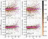 |
Fig. A.1. Difference between the flux difference (i.e. color gradient) between F115W−F150W (first column) and F150W−F356W (second column) computed using photometry from the Sérsic profile adding back the fit residuals (S+R) or just from the Sérsic profiles (S) measured within the effective radius Re, F444W (first row) or between 1 − 2 Re, F444W (second row). These are presented as a function of the global AV and color-coded with the galaxy redshift. White squares with magenta contour show the median difference in AV bins of width 0.2 mag, while error bars show the statistical uncertainty ( |

We note that for individual images the residuals are larger than for the colors: the covariance between the residuals in different filters reduces the impact on our color gradient estimates. Since residual corrections are very small (Fig. A.1) and can introduce new errors (PSF uncertainties affect the centers; noise peaks affect the low surface brightness outer parts), we choose to omit the residual corrections in this paper.
Appendix B: Estimate of the color gradient’s uncertainties
Color gradients presented in this work are computed by retrieving rest-frame U, V, J fluxes via SED fitting with the code EAZY. Random uncertainties are given by a combination of the observed flux uncertainties and model uncertainties - the underlying SED. Uncertainties provided by EAZY on the rest-frame fluxes include both. When computing color gradients, the covariant terms of the uncertainty on each band’s flux cancel out with the net effect that the final uncertainty is expected to be smaller than the simple quadrature sum of the uncertainties of all fluxes involved in the color gradient. In fact, covariant terms originate from the SED model, which affects the same way rest-frame fluxes computed at a fixed aperture. On the other hand, uncertainties on color gradients computed from observed fluxes are just given by the quadrature sum of the uncertainties on all the fluxes involved since no convolution with an SED model is involved in their determination.
To estimate the true uncertainty on color gradients, we compared the color gradients derived using rest-frame colors from EAZY (the same used throughout the paper) with color gradients computed using observed fluxes in the filters closest to the rest-frame bands investigated. The total scatter of the former (σEazy2) can be written as
 (B.1)
(B.1)
The constraint set in Section 2.3 that observations must overlap at least 50% of the rest-frame bands, combined with the statements of Brammer et al. (2011) who found colors retrieved with EAZY to accurately match colors retrieved by interpolating fluxes in nearby observed bands (when these overlap sufficiently with the rest-frame band), makes any bandpass mismatch errors negligible. The total scatter of the second (σOBS2) can be written as
 (B.2)
(B.2)
with σflux2 the scatter due to flux uncertainties, σcovariant2 the scatter due to covariance terms and σλ2 the scatter due to the difference in band coverage between the rest-frame band investigated and the closest filter. Since the sample is selected such that at least 50% of the area of the rest-frame band overlaps with observations, the scatter due to this term can be considered negligible compared to the others.
The scatter in the comparison between the two color gradients is then representative of the covariant term. Hence, the real uncertainty on EAZY color gradients used in this work can be computed as  where the latter term is represented by the scatter in Figure B.1 and is expressed a function of redshift.
To account also for the uncertainties of Re on the color gradients, we add in quadrature to σColorGrad a new term σSersic computed as the ratio between the fraction of light enclosed in the Sérsic profile tracing the U band up to Re, V that is the effective radius measured in the V band. The same is done for the V and J bands. This term accounts for the uncertainty induced by retrieving photometry from several different modeled Sérsic profiles and has a median value of σSersic, U − V ≈ 0.07 mag and σSersic, V − J ≈ 0.09 mag, comparable or smaller than the scatter shown in Figure B.1.
Appendix C: Color gradients and the wavelength dependence of size
A color gradient and a size difference measured at different wavelengths are (nearly) the same thing, especially when both derive from the same light profile fits. In fact, such size differences are often referred to as color gradients (i.e., Suess et al. 2022; Cutler et al. 2024; Ito et al. 2024; Ormerod et al. 2024; Martorano et al. 2024; Clausen et al. 2025). Specifically, in our previous work Martorano et al. (2024), we found a median optical-to-near-IR size ratio of 0.14 dex, and up to 0.25 dex for massive star-forming galaxies at z > 1.5. These results precisely mirror the color gradient trends analyzed in this paper, which aims at interpreting the origin of the color gradients (attenuation) rather than its effect on the measured structural evolution of galaxies. It is still useful to compare the color gradients, in this paper defined as the color difference between the outskirts (1 and 2Re) and the center (inside Re), with the size difference between the optical (rest-frame 0.5 μm) and near-IR (rest-frame 1.5 μm) from Martorano et al. (2024), even if both derive from the same Sérsic profile fits. In Figure C.1 we compare, for star-forming galaxies, the size differences with the V − J color gradients.
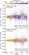 |
Fig. C.1. Comparison between the color gradients retrieved with EAZY rest-frame fluxes and observed fluxes as a function of redshift and color coded with the uncertainty on the color gradient retrieved using observed fluxes. The top panel shows the U − V color difference, while the bottom panel shows the V − J color difference. In the top left corner of each panel we present the median and standard deviation of the color gradient difference, while in the bottom right corner we show the median uncertainty on the two color gradients. Solid black lines show the standard deviation of the difference between the two color gradients as a function of redshift. |
There exists a strong correlation between the stellar mass and the size variation: low-mass galaxies have a median size variation of ≈25% while massive galaxies have median variations of ≈65%, as presented in Martorano et al. (2024). No clear redshift trend is recovered for any of the stellar mass bin investigated. By construction, this size difference closely correlates with our Δ(V − J), but there is substantial scatter that originates from variations in Sérsic index, that is the distribution of light within the two large apertures used to define the color gradient. A larger Sérsic index produces a larger size difference at a fixed color gradient (top row in Figure C.1). In addition, if the Sérsic index varies with wavelength (i.e., Kelvin et al. 2012; Vika et al. 2013; Kennedy et al. 2015; Martorano et al. 2023, 2025), then galaxies with strong color gradients may show just a mild difference in size and, vice versa, galaxies with mild color gradients may show strong size gradients (lower row in Figure C.1). The take-away message is that radial variations in color do not necessarily lead to net color gradient expressed as a summary statistic (here, comparing the average color between 1 and 2 Re with that inside Re as measured in F444W). Conversely, the lack of a color gradient as defined here, does not necessarily imply that the color is the same at all radii. The lack of a clear redshift trend in this figure proves that the size variation as a function of redshift presented in Martorano et al. (2024) is comparable to that presented in this work.
Sub-mm galaxies in our sample exhibit both strong color gradients and size variations (confirming results presented in Ren et al. 2025) that closely align with the median trends. These galaxies have median n1.5μm ≈ 1.3 and n0.5μm ≈ 1.1 confirming findings of Price et al. (2025), Gillman et al. (2024) and several others. As in Price et al. (2025), we find more concentrated sub-mm galaxies to have stronger size variation, suggesting galaxies with the most compact light distributions also have the most concentrated dust.
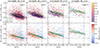 |
Fig. C.2. V − J color gradient vs relative size variation in four stellar mass bins. The two rows show the same data but color-coded respectively with the Sérsic index at 1.5 μm (top row) and the logarithm difference of Sérsic indices at rest-frame 1.5 μm and 0.5 μm (lower row). Just star-forming galaxies are shown. Diamonds show sub-mm-selected galaxies and are color-coded following the same color scheme of the other galaxies. Colored green lines show the running median in redshift bins. In the top right corner, we present the median uncertainties. Massive star-forming galaxies have systematically stronger size variation with wavelength and stronger color gradients than low-mass galaxies. The variation of the Sérsic index with wavelength correlates more strongly with the color gradient than with the size gradient. |
All Tables
All Figures
|
Fig. 1. Example of nine galaxies (field and DJA ID are shown left of each row) divided into three sets according to their stellar mass and ordered by redshift. For each galaxy, we present cutouts in the three filters that closely match the rest-frame U(blue)-V(green)-J(red) bands. The gray panels show the original images. To create the RGB images, each filter was first deconvolved with a Richardson-Lucy algorithm. We overplot ellipses with semimajor axis twice the effective radii measured in JWST/NIRCam F444W on the RBG image, as described in Sect. 2.2. |
| In the text | |
|
Fig. 2. Attenuation in the V band (AV) as a function of redshift in four stellar mass bins for star-forming galaxies color-coded with their V − J color. The white squares show the median in stellar mass bins, and the error bars show the statistical uncertainty ( |
| In the text | |
|
Fig. 3. UVJ plots for the same galaxies as in Figure 1. Each panel shows the UVJ color gradients in elliptical apertures with a width of 0.04″ up to an aperture of twice the effective radius in the filter F444W. The dashed black lines identify the quiescent region as defined by Muzzin et al. (2013). The white star with black contours shows the UVJ colors of the galaxy as in the DJA catalog, and the magenta (green) squares show the color measured within Re (1 − 2 Re). In the bottom right corner, we report the field and ID of the galaxy, together with its redshift, stellar mass, and global Av. In each panel, we show a metallicity and age grid from the BPASS stellar libraries, together with the theoretical AV vector induced by a dust screen. This figure shows different types of color gradients for the galaxies in the sample. |
| In the text | |
|
Fig. 4. Color gradients as a function of redshift for quiescent galaxies in four stellar mass bins and color-coded with global AV. The top row shows the U − V color gradients (Δ(U − V) = (U − V)1 < r/Re < 2 − (U − V)r < Re), and the bottom row shows the V − J color gradients (Δ(V − J) = (V − J)1 < r/Re < 2 − (V − J)r < Re). The black error bars in the lower left (right) corner of each panel show the median uncertainty on the color gradients for all the galaxies in that stellar mass bin with z < 1.5 (z > 1.5). The solid black lines show the running median, and the dashed lines show the 16−84 percentile range. The squares show the median color in redshift bins with a width of 0.25, and the (generally negligible) error bars represent the statistical uncertainty |
| In the text | |
|
Fig. 5. Same as Fig. 4, but for star-forming galaxies. The diamonds identify submillimeter-selected galaxies. The black error bars in the lower part of each panel show the median uncertainty on the color gradients at that redshift. Δ(U − V) show no discernible redshift dependence and low-mass galaxies show no U − V gradients at z > 1.5. Conversely, Δ(V − J) shows a strong mass and redshift dependence. |
| In the text | |
|
Fig. 6. UVJ diagram of the colors measured within the F444W effective radius, with hexbins containing at least five galaxies color-coded with the median global AV. The length and direction of the arrows indicate the median color shift from within the effective radius to the aperture between 1 Re and 2 Re, following our definition of a color gradient throughout this paper. A minimum of ten galaxies in the hexbin was required for drawing an arrow. The green diamonds highlight the U − V and V − J colors within 1 Re for the submillimeter-selected sample. |
| In the text | |
|
Fig. 7. Projected axis ratio (q) observed in JWST/NIRCam-F444W against U − V (upper panels) and V − J (lower panels) colors in four redshift bins. The color-coding shows the color gradient computed as the difference between the color between 1−2 Re and 0−1 Re. We only show quiescent galaxies with stellar mass M★ ≥ 1010.5 M⊙. In the lower left corner, we show the median uncertainties on the rest frame colors and axis ratios and the Spearman correlation coefficient between the axis ratio and the color, and in the right corner, we show that between the axis ratio and the color gradient. |
| In the text | |
|
Fig. 8. Same as Figure 7, but for M★ ≥ 1010.5 M⊙ star-forming galaxies. The diamonds show submillimeter-selected galaxies. The correlation between the colors and q decreases with redshift. |
| In the text | |
|
Fig. A.1. Difference between the flux difference (i.e. color gradient) between F115W−F150W (first column) and F150W−F356W (second column) computed using photometry from the Sérsic profile adding back the fit residuals (S+R) or just from the Sérsic profiles (S) measured within the effective radius Re, F444W (first row) or between 1 − 2 Re, F444W (second row). These are presented as a function of the global AV and color-coded with the galaxy redshift. White squares with magenta contour show the median difference in AV bins of width 0.2 mag, while error bars show the statistical uncertainty ( |
| In the text | |
|
Fig. C.1. Comparison between the color gradients retrieved with EAZY rest-frame fluxes and observed fluxes as a function of redshift and color coded with the uncertainty on the color gradient retrieved using observed fluxes. The top panel shows the U − V color difference, while the bottom panel shows the V − J color difference. In the top left corner of each panel we present the median and standard deviation of the color gradient difference, while in the bottom right corner we show the median uncertainty on the two color gradients. Solid black lines show the standard deviation of the difference between the two color gradients as a function of redshift. |
| In the text | |
|
Fig. C.2. V − J color gradient vs relative size variation in four stellar mass bins. The two rows show the same data but color-coded respectively with the Sérsic index at 1.5 μm (top row) and the logarithm difference of Sérsic indices at rest-frame 1.5 μm and 0.5 μm (lower row). Just star-forming galaxies are shown. Diamonds show sub-mm-selected galaxies and are color-coded following the same color scheme of the other galaxies. Colored green lines show the running median in redshift bins. In the top right corner, we present the median uncertainties. Massive star-forming galaxies have systematically stronger size variation with wavelength and stronger color gradients than low-mass galaxies. The variation of the Sérsic index with wavelength correlates more strongly with the color gradient than with the size gradient. |
| In the text | |
Current usage metrics show cumulative count of Article Views (full-text article views including HTML views, PDF and ePub downloads, according to the available data) and Abstracts Views on Vision4Press platform.
Data correspond to usage on the plateform after 2015. The current usage metrics is available 48-96 hours after online publication and is updated daily on week days.
Initial download of the metrics may take a while.