| Issue |
A&A
Volume 705, January 2026
|
|
|---|---|---|
| Article Number | A173 | |
| Number of page(s) | 21 | |
| Section | Extragalactic astronomy | |
| DOI | https://doi.org/10.1051/0004-6361/202556574 | |
| Published online | 19 January 2026 | |
JWST spectroscopic confirmation of the Cosmic Gems arc at z = 9.625
Insights into the small-scale structure of a post-burst system
1
INAF – OAS, Osservatorio di Astrofisica e Scienza dello Spazio di Bologna Via Gobetti 93/3 I-40129 Bologna, Italy
2
Department of Astronomy, Oskar Klein Centre, Stockholm University, AlbaNova University Centre SE-106 91 Stockholm, Sweden
3
Center for Frontier Science, Chiba University, 1-33 Yayoi-cho Inage-ku Chiba 263-8522, Japan
4
Department of Physics, Graduate School of Science, Chiba University, 1-33 Yayoi-Cho Inage-Ku Chiba 263-8522, Japan
5
Department of Astronomy, University of Michigan 1085 South University Avenue Ann Arbor MI 48109, USA
6
Space Telescope Science Institute 3700 San Martin Drive Baltimore MD 21218, USA
7
Niels Bohr Institute, University of Copenhagen Jagtvej 128 2200-N Copenhagen, Denmark
8
Cosmic Dawn Center (DAWN), Denmark
9
Univ Lyon, Univ Lyon1, ENS de Lyon, CNRS, Centre de Recherche Astrophysique de Lyon UMR5574 Saint-Genis-Laval, France
10
Center for Astrophysical Sciences, Department of Physics and Astronomy, The Johns Hopkins University 3400 N Charles St. Baltimore MD 21218, USA
11
Instituto de Alta Investigación, Universidad de Tarapacá Casilla 7D Arica, Chile
12
Dipartimento di Fisica, Università degli Studi di Milano Via Celoria 16 I-20133 Milano, Italy
13
Max-Planck-Institut für Astrophysik Karl-Schwarzschild-Str. 1 D-85748 Garching, Germany
14
INAF – IASF Milano Via A. Corti 12 I-20133 Milano, Italy
15
University of Ljubljana, Faculty of Mathematics and Physics Jadranska ulica 19 SI-1000 Ljubljana, Slovenia
16
Instituto de Física de Cantabria (CSIC-UC) Avda. Los Castros s/n. 39005 Santander, Spain
17
Center for Astrophysics | Harvard & Smithsonian 60 Garden Street Cambridge MA 02138, USA
18
Department of Physics, School of Advanced Science and Engineering, Faculty of Science and Engineering, Waseda University 3-4-1 Okubo Shinjuku Tokyo 169-8555, Japan
19
Waseda Research Institute for Science and Engineering, Faculty of Science and Engineering, Waseda University 3-4-1 Okubo Shinjuku Tokyo 169-8555, Japan
20
David A. Dunlap Department of Astronomy and Astrophysics, University of Toronto 50 St. George Street Toronto Ontario M5S 3H4, Canada
21
Dunlap Institute for Astronomy and Astrophysics 50 St. George Street Toronto Ontario M5S 3H4, Canada
22
Department of Astronomy, University of Maryland College Park 20742, USA
23
Dipartimento di Fisica e Scienze della Terra, Università degli Studi di Ferrara Via Saragat 1 I-44122 Ferrara, Italy
24
Astrophysics Science Division, Code 660, NASA Goddard Space Flight Center 8800 Greenbelt Rd. Greenbelt MD 20771, USA
25
School of Earth and Space Exploration, Arizona State University Tempe AZ 85287-1404, USA
26
Center for Interdisciplinary Exploration and Research in Astrophysics (CIERA) 1800 Sherman Avenue Evanston IL 60201, USA
27
Observational Astrophysics, Department of Physics and Astronomy, Uppsala University Box 516 SE-751 20 Uppsala, Sweden
28
INAF Osservatorio Astronomico di Padova vicolo dell’Osservatorio 5 35122 Padova, Italy
29
Department of Physics, Ben-Gurion University of the Negev P.O. Box 653 Be’er-Sheva 84105, Israel
★ Corresponding author: This email address is being protected from spambots. You need JavaScript enabled to view it.
Received:
24
July
2025
Accepted:
31
October
2025
Abstract
We present JWST/NIRSpec integral field spectroscopy of the Cosmic Gems arc, strongly magnified by the galaxy cluster SPT-CL J0615−5746. Six-hour integration using NIRSpec prism spectroscopy (resolution R ≃ 30 − 300), covering the spectral range 0.8 − 5.3 μm, reveals a pronounced Lyα-continuum break at λ ≃ 1.3 μm, as well as weak optical Hβ and [O III] λ4959 emission lines at z = 9.625 ± 0.002, located in the reddest part of the spectrum (λ > 5.1 μm). No additional ultraviolet or optical emission lines are reliably detected. A weak Balmer break is measured alongside a very blue ultraviolet slope (β ≤ −2.5, Fλ ∼ λβ). Spectral fitting with Bagpipes suggests that the Cosmic Gems galaxy is in a post-starburst phase, making it the highest-redshift system currently observed in a mini-quenched state. Spatially resolved spectroscopy at tens of parsecs shows relatively uniform features across subcomponents of the arc. These findings align well with the physical properties previously derived from JWST/NIRCam photometry of the stellar clusters, now corroborated by spectroscopic evidence. In particular, five observed star clusters exhibit ages of 7 − 30 Myr. An updated lens model constrains the intrinsic sizes and masses of these clusters, confirming they are extremely compact and denser than typical star clusters in local star-forming galaxies (ΣM★ = 105 − 106 M⊙). Additionally, four compact stellar systems consistent with star clusters (≲10 pc) are identified along the extended tail of the arc. A sub-parsec line-emitting HII1.2ex region straddling the critical line, lacking a NIRCam counterpart, is also serendipitously detected. The Cosmic Gems arc thus offers a rare opportunity to investigate, at parsec scales, the aftermath of a star formation burst in the early Universe.
Key words: gravitational lensing: strong / HII regions / galaxies: high-redshift / galaxies: star clusters: general / galaxies: star formation
© The Authors 2026
 Open Access article, published by EDP Sciences, under the terms of the Creative Commons Attribution License (https://creativecommons.org/licenses/by/4.0), which permits unrestricted use, distribution, and reproduction in any medium, provided the original work is properly cited.
This article is published in open access under the Subscribe to Open model. This email address is being protected from spambots. You need JavaScript enabled to view it. to support open access publication.
1. Introduction
One of the major surprises of surpassing the first half-gigayear threshold in cosmic time (corresponding to z > 9) is the significant slow evolution of the space density of bright galaxies (e.g., Finkelstein et al. 2024; Napolitano et al. 2025). The discovery and subsequent confirmation of a substantial population of bright z > 9 galaxies (typically with MUV < −20) by JWST observations have now well established this trend (e.g., Naidu et al. 2022; Arrabal Haro et al. 2023; Hsiao et al. 2024; Wang et al. 2023; Fujimoto et al. 2024; Atek et al. 2023; Curtis-Lake et al. 2023; Robertson et al. 2023; Bunker et al. 2023; Tacchella et al. 2023; Arrabal Haro et al. 2023; Finkelstein et al. 2024; Castellano et al. 2024; Zavala et al. 2025; Helton et al. 2025; Carniani et al. 2024; Robertson et al. 2024; Tang et al. 2025; Donnan et al. 2025). Several physical mechanisms have been discussed to explain this phenomenon, including a top-heavy initial mass function (e.g., Trinca et al. 2024; Hutter et al. 2025), extremely bursty star formation histories (SFHs, Mason et al. 2023; Pallottini & Ferrara 2023; Garcia et al. 2025; Carvajal-Bohorquez et al. 2026), reduced feedback resulting in higher star formation efficiency (e.g., Dekel et al. 2023; Li et al. 2024; Somerville et al. 2025), radiation-driven feedback processes (Ferrara et al. 2023, 2025a; Sugimura et al. 2024), or a combination thereof.
Efforts are now underway to extend these studies to fainter galaxies at similar redshifts (e.g., Atek et al. 2024; Mowla et al. 2024; Tang et al. 2025; Whitler et al. 2025, and upcoming observations, e.g., the cycle 4 Vast Exploration for Nascent, Unexplored Sources (VENUS) large program, GO-6882, PI Fujimoto). The confirmation of very high-redshift galaxies primarily relies on the detection of either strong emission lines or a continuum break, the latter being feasible only for intrinsically bright sources. These techniques have led to the confirmation of the most distant known galaxies to date at z = 14.2 (Carniani et al. 2024) and z = 14.44 (Naidu et al. 2025).
Accessing the population of faint and weakly (or non-) emitting galaxies at z > 9 is therefore the next frontier. These include galaxies in a post-burst or off-mode phase of star formation (SF), sometimes referred to as mini-quenched galaxies (e.g., Gelli et al. 2023; Dome et al. 2024; Endsley et al. 2025, 2024; Topping et al. 2024; Looser et al. 2024, 2025; Baker et al. 2025; Covelo-Paz et al. 2025), observed a few tens of megayears after a starburst. If SFHs in the early Universe are generally bursty, especially at low masses, then we may expect many high-z galaxies to be in a temporary “dormant” post-burst phase (Tacchella et al. 2016, 2020; Faucher-Giguère 2018; Sun et al. 2023a,b; Mason et al. 2023; Garcia et al. 2023). In such systems, the most massive O-type stars have already evolved, reducing the ionizing output and leading to weak or absent emission lines (e.g., Stasińska & Leitherer 1996; Choi et al. 2017), which makes detailed spectroscopic characterization particularly difficult (e.g., Looser et al. 2025). As the equivalent width (EW) of nebular emission lines decreases, only the continuum break constrains the redshift. This requires very long or impractical exposure times, even with instruments such as JWST/NIRSpec. One of the most effective strategies to overcome this difficulty involves leveraging gravitational lensing, which enables the spectroscopic confirmation of z > 9 galaxies with MUV > −20 (e.g., Roberts-Borsani et al. 2023).
The Cosmic Gems arc (Salmon et al. 2018; Strait et al. 2020; Welch et al. 2023; Adamo et al. 2024; Bradley et al. 2025) provides a unique case at z ≃ 10, where gravitational lensing magnifies a relatively faint source (intrinsic MUV ≃ −18.4, apparent delensed magnitude mUV ≃ 29.1) into a bright arc with an observed magnitude F200W = 24.5 (Bradley et al. 2025). In addition to the enhanced signal-to-noise ratio provided by lensing, the strong tangential stretching has resolved internal substructures, allowing the identification of five massive, dense star clusters (Adamo et al. 2024), along with fainter components extending along the arc’s tail. While a detailed analysis of the star cluster mass function and its connection to the counterimage is presented in a companion paper Vanzella et al. (2026, hereafter V25), here we report on JWST/NIRSpec integral field units (IFU) spectroscopy of the bright arc. These observations provide an exceptionally high S/N redshift confirmation, despite the presence of relatively weak spectral features. This fortunate configuration enables us to spatially resolve and analyze both the star clusters and the host galaxy, offering a rare window into a post-burst system at the epoch of reionization.
This paper is structured as follows: Observations and data reduction are outlined in Section 2. The updated lens models used in this work are described in Section 3. The spectral analysis of the Cosmic Gems and the study of its star cluster population are presented in Sections 4 and 5, respectively. Finally, the main results are discussed in Section 6 and summarized in Section 7.
Throughout this paper, we adopt a flat Lambda cold dark matter (Λ-CDM) cosmology with H0 = 70 km s−1 Mpc−1 and ΩM = 0.3, a Kroupa (2001) initial mass function, and a solar metallicity Z⊙ = 0.02. All quoted magnitudes are in the AB system. All quoted EWs are rest-frame values.
2. Observations and data reduction
2.1. JWST-NIRSpec
JWST/NIRSpec IFU observations (GO 5917, PI: Vanzella) targeting the strongly lensed Cosmic Gems arc, magnified by the galaxy cluster SPT-CL J0615−5746 (hereafter SPT0615) were acquired on February 4, 2025. Figure 1 shows the layout of the field of view, which includes the major emitting mirrored regions A, B, C, D, E groups 1 and 2, along with the tail of the arc oriented toward the north. A total integration time of ≃5.8 hours on target were acquired. The dataset consists of PRISM spectroscopy covering the spectral range 0.8 − 5.3 μm, with spectral resolution varying from R ≃ 30 (around ∼1 μm) to R ≃ 300 (at the longest wavelengths).
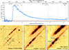 |
Fig. 1. JWST/NIRSpec spectrum, NIRCam, and pseudo-NIRCam images (NIRSpec-IFU based) of the Cosmic Gems arc. Top: 1D NIRSpec prism spectrum (from the PSF-matched cube) extracted from the full arc (with its aperture mask shown in the bottom-central panel), showing the large Lyα-break and damping at ≃1.3 μm, along with two weak emission lines, Hβ and [O III] λ4959, on the rightmost side of the spectral range. A weak Balmer break is also detected (Section 4). The 1σ uncertainty spectrum is shown in red. The wavelengths corresponding to the main undetected UV and optical lines are shown with dashed lines. The throughputs of the NIRCam filters covering the field are shown in green, for reference. Bottom: From left to right, JWST/NIRCam stacked F150W + F200W image with the NIRSpec-IFU field of view outlined; collapsed NIRSpec IFU data cube in the rest-UV (covering the observed wavelength range of F150W and F200W), before (middle) and after (right) PSF-matching. The last panel also includes the outlines of the masks used to extract the 1D spectra for the regions discussed in the main text. |
The data were reduced following the same procedures described in Messa et al. (2025) (see also Vanzella et al. 2024). Briefly, we used the STScI pipeline (v1.17.0 and 1322.pmap, Bushouse et al. 2023) and post-processed the intermediate products of stage 2 with customized procedures that combine the eight partial cubes into the final cleaned cube. The latter included background subtraction, removal of detector defects, and the computation of the error spectrum. Additionally, we performed the 1/f noise subtraction in stage 1 using the clean_flicker_noise step. In contrast with the faint targets discussed in Messa et al. (2025), the Cosmic Gems arc was well detected in the continuum at each wavelength slice; therefore, we estimated the background at each wavelength by computing a 2D polynomial fitting in regions of the field of view free from clearly detected sources (see Appendix A). The zero, first, and second-order polynomial fittings produce similar results. We used the first-order fit as fiducial background subtraction. As in Messa et al. (2025), the error cube was derived by storing the median deviation of each pixel from the combination of the partial cubes.
We produced data cubes at 100 and 50 milli-arcsec (mas) per pixel. By comparing 1D spectra coming from the same regions of the arc, we found no notable differences (Appendix A); therefore, we decided to keep the 50 mas reduction as our reference, as it better samples the NIRSpec PSF. Flux calibration was cross-checked with JWST/NIRCam photometry extracted from the main target Cosmic Gems arc (Bradley et al. 2025). The detected sources (the arc and the nearby z = 2.5 galaxy) in the reduced, post-processed, and collapsed data cubes were aligned with their JWST/NIRCam counterparts.
We checked the consistency of the above products with an independent reduction carried out from stage 3 of the official pipeline. Overall, the results are fully consistent, with the above post-processing producing slightly cleaner spectra (reduced spikes and defects; see Appendix A).
Finally, we PSF-matched the data in the spectral wavelength using as reference the PSF models produced by the STPSF tool1 (assuming the same instrumental configurations as our data). The modeled PSF as a function of wavelength shows good agreement with the PSF recovered by fitting the shape of one of the bright sources in our field-of-view (see Appendix A). The final data cube was matched to the worst PSF at 5.3 micron, applying a kernel smoothing at each wavelength slice2, following the aforementioned PSF variation trend. The bottom panels in Figure 1 show a collapsed 1.3–2.3 μm image of the rest-frame UV part of the IFU cube before and after the PSF-matching of the cube. This correction was implemented in order to avoid a wavelength-dependent loss of flux when extracting 1D spectra from the IFU masks (Section 4). The 1D spectrum (and relative uncertainty) coming from the final reduction is shown in Figure 1.
Throughout the paper we refer to the image and cluster notation introduced in Adamo et al. (2024) and Bradley et al. (2025), i.e., the galaxy’s image in the southeast is numbered “1” while the one in the northwest “2”, and clusters are named “A” to “E” (see bottom-left panel in Fig. 1). The NIRCam imaging used in this work (Figs. 1, 3, 6 and 7) is presented in Bradley et al. (2025).
2.2. VLT-MUSE
SPTJ0615 was observed with the MUSE instrument on the VLT between January and March 2024 (period P112, PI: F. Bauer) in the wide field mode (WFM) and using the adaptive optics (WFM-AO-N). The observations consist of 6.2 hours of observing time in total (24 individual exposures of 930 seconds each), divided into two different pointings covering the core of the cluster. The MUSE data reduction was performed using the same procedure described in Richard et al. (2021), largely following the prescription described in Weilbacher et al. (2020), with some specific improvements for crowded fields. The final output is given as an FITS data cube with two extensions containing the flux and the associated variance over a regular 3D grid at a spatial pixel scale of  and a wavelength step of 1.25 Å between 4750 and 9350 Å. The use of the AO mode results in a gap in the 5800–5980 Å wavelength range due to the AO notch filter. Individual exposures were aligned against each other and with respect to four star positions in J2000 selected from the Gaia data release 2 (Gaia Collaboration 2018). The relative astrometry between the MUSE cube and the HST images was cross-checked by matching bright sources present in the two datasets. We measure a alignment rms of 0.1″, corresponding to half a MUSE spaxel. Following the same method as Richard et al. (2021), a line-detected sources catalog was produced directly from the MUSE data cube, performed by running the muselet software, which is part of the MPDAF Python package (Piqueras et al. 2019).
3. Updated lens model
We present updated mass models (with respect to what presented in Adamo et al. 2024 and Bradley et al. 2025) constructed with both glafic (Oguri 2010, 2021) and Lenstool (Jullo et al. 2007). A panoramic view of the lensing cluster SPT0615 is given in Fig. 2, along with the critical lines predicted by the two lens models at the redshift of the target. In this work, we refer to the magnification values obtained by the glafic model as the reference ones, but we provide a one-to-one comparison of the two models in Appendix B. This direct comparison between the two models – revealing differences of up to a factor of ∼1.5 – provides insight into the systematic uncertainties that are typically not captured by the statistical uncertainties of the individual models. Overall, the updated magnification values along the Cosmic Gems arc remain similar to the ones used in Adamo et al. (2024) and Bradley et al. (2025).
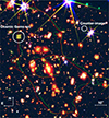 |
Fig. 2. JWST/NIRCam color image of the galaxy cluster SPT0615 field with the locations of the Cosmic Gems arc and its counter-image marked, along with the critical lines for the z = 9.625 lens models from LENSTOOL (red line) and glafic (green line). The yellow-shaded square marks the field of view of the JWST/NIRSpec IFU observations. |
3.1. Multiple image catalog
The updated models adopt 54 multiple images from 18 sources. Among the 18 sources, 12 have spectroscopic redshifts. In this paper, we identify 12 new multiple images from four sources. In addition to the new spectroscopic redshift for the Cosmic Gems arc from JWST, we add spectroscopic redshifts for four sources from our MUSE spectroscopy (see Section 2.2). Photometric redshift estimates were used for four of the sources without spectroscopic redshift. Finally, for two sources (five multiple images in total) the redshift was left as a free parameter. The details of the multiple images are summarized in Appendix B. The inclusion of newly identified multiple systems at z ≳ 6, located near the observed position of the Cosmic Gems, strengthens the constraints and improves the robustness of the updated lens models in the region of the arc.
3.2. Glafic model
The updated glafic mass model assumes the positional error of  for the multiple images (including the counter image of the Cosmic Gems arc), except for the Cosmic Gems arc for which the smaller position error of
  is assumed to accurately reproduce the positions of the image clusters. The complex dark matter distribution of this cluster is modeled by four elliptical Navarro–Frenk–White (hereafter NFW, Navarro et al. 1997) components. For the first three NFW components, their centers were fixed at (93.9656010, −57.7801990), (93.9705078, −57.7753866), and (93.9613773, −57.7810248) where bright cluster member galaxies are located, while the center of the remaining NFW component was fit to the data. The best-fitting position of this NFW component is (93.9519126, −57.7804012). In addition to the NFW components, we included the external shear, the third-order multipole perturbation, and cluster member galaxies. The latter are modeled by elliptical pseudo-Jaffe ellipsoids with ellipticities and position angles fixed to observed shapes of galaxies. The three parameters modeling the scaling relation of pseudo-Jaffe ellipsoids and galaxy luminosities were treated as free parameters (see, e.g., Kawamata et al. 2016). The mass model was optimized by minimizing the chi-squared statistic evaluated in the source plane, taking account of the full magnification tensor (see Appendix 2 of Oguri 2010). The best-fitting mass model has a root-mean-square between observed and model-predicted multiple image positions of
  , and χ2 = 37.2 for 45 degrees of freedom. We ran a Markov chain Monte Carlo (MCMC) to derive errors on model-predicted quantities such as magnification.
To check the robustness of the identification of the counter-image of the Cosmic Gems arc at (93.95000, −57.77023) used as a constraint in our default setup, we also derived another glafic mass model excluding the counter-image. This model predicts the position of the counter-image at (93.94978, −57.77004), i.e.,  away from the observed position, with a 1σ error of
  . Therefore, this model correctly predicts the observed counter-image position within about 1σ level, which confirms the robustness of the identification of the counter-image (see also V25). From the magnification map at the redshift of the Cosmic Gems (z = 9.625, see Section 4.1), we extracted amplification values for the subregions of interest using small apertures at their observed positions (see Appendix B for more details).
3.3. Lenstool model
Lenstool uses a parametric approach to model the foreground lens, and MCMC to explore the parameter space, identify the best-fit parameters, and estimate uncertainties. Our lens modeling strategy follows Sharon et al. (2020). We optimized the parameters of three halos, one associated with the mass of the cluster, one fixed to the position of the brightest cluster galaxy (BCG), and a third halo to allow contribution to the lensing potential from a foreground group. Cluster-member galaxies were selected using the red sequence technique (Gladders & Yee 2000). We used the dual pseudo-isothermal elliptical (dPIE) mass distribution with seven parameters, x, y, e, θ, rcut, rcore, and σ0. The cut radius was fixed at 1500 kpc for the two cluster-scale halos. The mass associated with galaxies was linked to their magnitudes through scaling relations (Jullo et al. 2007), and their positional parameters were fixed to the observed light distribution. As constraints, we used the positions of multiple images of emission clumps, and the spectroscopic redshifts of sources (Appendix B). Where a spectroscopic redshift was not available, the redshift of the source was left as a free parameter with broad priors. The positional uncertainty of all multiple image constraints was assumed to be  . Finally, we used a positional constraint on the critical curve (CC) crossing of the arc, with a positional uncertainty set to
  . Similar to the glafic analysis, we produced two lens models: model A used the counter image of the Cosmic Gems arc as a constraint, and model B did not.
We used 21 free parameters and 70 (68) constraints for the model with (without) the counter image constraint. Model A resulted in an image-plane RMS of  , reducing to
  for model B. The image-plane RMS of the four clumps along the arc ranges from
  to
to  , implying a high precision in this region. The model-A predicted position of the counter-image is
  from the observed counter image, at [
 ,
,  ]. Uncertainties on model predictions were derived by sampling 250–280 steps from the MCMC and computing lensing outputs (e.g., magnification) from these sets of parameters.
4. NIRSpec analysis of the arc
To extract 1D spectra from the IFU cube and investigate the sub-galactic regions of the Cosmic Gems, we defined six mask apertures (Fig. 1, bottom-right panel), taking into account the identification of unique morphological features and NIRSpec resolution. The two images of cluster A were covered with individual masks (A1 and A2), as they are bright isolated sources. On the other hand, the rest of the clusters were unresolved with the NIRSpec PSF and were observed as a single elongated source. We defined a mask that covers the entire region containing clusters B–E (BCDE1 and BCDE2 for the two images). The narrow region between clusters E.1 and E.2, where the CC crosses the arc, was covered with a further mask (CC). The faint tail of the arc was covered by the TAIL mask. In the following analyses, we sometimes consider that the flux from two mirrored regions combined (e.g., BCDE1,2 contains the flux from both BCDE1 and BCDE2). Finally, a mask aperture covering the entire image 2 of the arc (ARC2) is used for the analysis in Section 4.6, and an even larger one covering the full arc (ARC1,2) was used to extract the spectrum shown in Fig. 1. Spectra extracted from the aforementioned mask apertures are shown in Appendix C.
4.1. Spectroscopic redshift and emission map
The 1D spectrum of the Cosmic Gems (Fig. 1) is characterized by the clear Lyα break, used in previous publications to constrain photometrically the redshift of the system (zphot = 10.2, Bradley et al. 2025) and by two faint emission lines, which we identify as Hβ and [O III] λ4959. The spectroscopic redshifts derived from the two lines are zHβ = 9.625 ± 0.002 and z[OIII] = 9.630 ± 0.001. Their redshift difference (consistent within 3σ) is well within the spectral resolution at ∼5 μm3. We decided to keep zHβ = 9.625 as the reference redshift of the Cosmic Gems galaxy, due to the [O III] λ4959 line being very close to the edge of the wavelength range detected (the red tail of the line was excluded from the fit, as shown in Fig. 3).
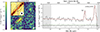 |
Fig. 3. Left: 2D map of the stacked Hβ + [O III] λ4959 in the wavelength range 5.15–5.3 μm (see text for more details). The red mask corresponds to the regions BCDE1,2 and CC (defined in Fig. 1), used to extract the spectrum on the right. The inset shows the NIRCam F150W + F200W data with overlaid black contours showing the peak of the Hβ + [O III] λ4959 emission and the CCs from GLAFIC (blue) and Lenstool (red). The white circle (in both the map and the inset) denote the FWHM of the NIRSpec-IFU PSF, while the NIRCam one is plotted as a black circle in the inset. Right: 1D spectrum (thick gray line) in the wavelength range of the detected emission lines. The continuum and line best-fitting result are shown as a red line. The error spectrum and spectral fit residuals are shown in green and light gray, respectively. The gray bands mark the portion of the spectrum not included in the fit. |
The spectroscopic redshift is lower than the photo-z previously published by Bradley et al. (2025). The main reason behind this difference seems to be the part of the spectrum affected by strong Lyα-damping wings. The shape of the observed spectrum is not accurately described by the sharp drop given by the intergalactic medium (IGM) absorption prescriptions by Inoue et al. (2014), adopted as standard prescription in the EAZYPY, (Brammer et al. 2008) photo-z fitting code used in Bradley et al. (2025)4. This effect has been widely discussed in the literature (e.g., Fujimoto et al. 2023; Finkelstein et al. 2024; Hainline et al. 2024; Heintz et al. 2025). A deeper analysis of the Lyα damping along the Cosmic Gems arc was performed in a separate study (i.e., Christensen et al., in prep.) and is briefly discussed also in the appendix of V25. In brief, a very strong damping wing from hydrogen absorption is observed in the regions occupied by the clusters (A and BCDE), revealing high hydrogen column densities, log N(HI1.2ex)/[cm−2]∼22.4. Densities an order of magnitude lower are found in the more diffuse regions of the arc (i.e., the TAIL).
We created emission-line maps of Hβ and [O III] λ4959 by collapsing the spectral channels including the lines, after continuum subtraction. For each pixel, the continuum level was estimated as the median of the slices in the (observed) wavelength range 5.20–5.24 μm. The slices containing the lines are in ranges 5.16–5.18 and 5.27–5.29 μm for Hβ and [O III] λ4959, respectively. The individual emission-line maps were combined in a Hβ + [O III] λ4959 map shown in Fig. 3 (left panel). The ionized gas emission is located in proximity of the critical line intersecting the arc, and it extends partly toward the BCDE region. The spectral wavelengths containing the emission lines from this region of larger emission (combining the masks of BCDE1,2 and CC, visualized as a red contour in the left panel), are shown in Fig. 3 (right panel). The best fit of this spectrum (red line), modeled as the combination of a linear continuum and two Gaussian lines, was used to determine the spectroscopic redshift quoted above.
4.2. BCDE regions
4.2.1. Main spectral features
We extracted the spectrum for the region occupied by clusters B, C, D, and E from the BCDE1 and BCDE2 aperture masks shown in Fig. 1. The stacked spectrum from both regions (dubbed BCDE1,2) is shown in Fig. 4. We extracted three main features of the spectrum, namely the EW of the emission lines, the Balmer break (Bb), and the UV slope (βUV). All are reported in Appendix D. The EWs of Hβ and [O III] λ4959 were derived by simultaneously fitting a linear continuum and two Gaussians to the observed spectrum, as in Section 4.1, to derive the redshift of the galaxy. The resulting rest-frame EW values are EW([O III] λ4959)  and EW(Hβ)
  . By assuming the intrinsic ratio of the [O III] lines (λ5007/λ4959 = 2.98), we derived the expected flux in [O III] λ5007 and consequently the R3≡ [O III] λ5007/Hβ ratio. The value R3 = 7.5 ± 1.8, suggests that the metallicity of the galaxy is in the range Zgas ∼ 10 − 20% Z⊙ (assuming standard R3 metallicity calibrations, e.g., Nakajima et al. 2022; Sanders et al. 2024, 2025).
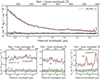 |
Fig. 4. Spectrum of the combined BCDE12 regions (gray), along with the best-fit model (red), residuals (black), and ±1σ uncertainties (green). Bottom panels: Zoom-ins on the regions where the best-fit predicts the main emission lines. |
Following the prescription used in Binggeli et al. (2019) and Endsley et al. (2025), we quantified the Balmer break amplitude as Fν(4200 Å)/Fν(3500 < Å). In order to mitigate the variability of monochromatic values, we considered the fluxes averaged over the rest-frame ranges from 4050 to 4330 Å and from 3290 to 3580 Å. A significant break was recovered, (Bb: 1.3 ± 0.1). Finally, the rest-UV slope was fit in the range from 1600 to 2600 Å, avoiding the wavelength region close to the Lyα damping in the blue part. The best-fit value, βUV = −2.53 ± 0.03, is steep but in line with average UV slopes found in z ≳ 8 galaxies (e.g., Cullen et al. 2023; Donnan et al. 2025; Tang et al. 2025).
The values derived for the main spectral features (summarized in Appendix D) provide a powerful insight into the age of the system and of its SFH (following e.g., Endsley et al. 2025). We can assume two extreme and opposite SFH cases, namely a constant star formation and an instantaneous burst (single stellar population, SSP), encompassing more complex SFHs evaluated below. In spite of the SFH assumption, the steep UV slope requires the system to be younger than ≲30 Myr in the two cases (assuming no extinction). On the other hand, the relatively low EWs (the total value for the sum of the Hβ + [O III] lines5 is 198 Å) imply an age ≳7 Myr for an SSP, and much older (≳500 Myr) for constant SFHs. The small Balmer break observed is also consistent with a stellar age in the range ∼10 − 20 Myr, in the SSP case. Long SFHs are disfavored, as the old ages required to explain the observed Bb and EWs under this assumption (up to ≳500 Myr for a constant SF) are incompatible with the observed blue UV slope.
An absorption feature was detected in the spectrum near the expected wavelength of CIV λλ1548, 1550 Å. The absorption peak was observed at 1.628 μm, where the prism mode provides its lowest spectral resolution (R ∼ 40), corresponding to ∼10 000 km s−1. Assuming this feature arises from CIV absorption, it would be blueshifted relative to the systemic redshift (as traced by optical emission lines) by Δv ≃ −3200 km s−1(see Appendix C). Given the large blueshift, the relatively low signal-to-noise ratio, and the limited spectral resolution at 1.6 μm, we caution against a definitive interpretation of the presence of the CIV doublet in absorption. Higher spectral resolution spectroscopy is necessary to confirm this feature and, more generally, to investigate the potential presence of faint, narrow ultraviolet emission and/or absorption lines.
4.2.2. Spectral fitting
To further constrain the intrinsic properties of the region, we fit the spectrum with Bagpipes (Carnall et al. 2018, 2019), using BPASS stellar models (Eldridge et al. 2017; Stanway & Eldridge 2018), assuming a delayed exponentially decaying SFH and leaving the following free parameters: the age and the exponential index of the SFH (τ); the stellar mass formed and its metallicity; the extinction AV (with the Calzetti et al. 2000 attenuation law assumed); and the ionization parameter log(U). Redshift was allowed to vary within the range 9.625–9.630, to account for the slight redshift difference between the two observed lines (see Section 4.1). To account for possible underestimation, the spectral uncertainties were left free to be scaled by up to a factor of 50. We used flat priors in the logarithmic space for all parameters excluding the extinction. Finally, the velocity dispersion was left as a free parameter. We point out that the Bagpipes model spectra were adjusted to match the line spread function of the NIRSpec observations, before fitting. We restricted the fit to wavelengths longer than 1600 Å rest-frame (1.7 μm observed) to avoid the part affected by Lyα damping. The spectrum and best-fit model are shown in Fig. 4. The model nicely reproduces the two emission lines, the small Balmer break and the UV slope. It also suggests the possible presence of other emission lines, namely Hγ, [O II] λλ3727, 3729 and [Ne III] λ3869. We zoom-in on their respective regions of the spectrum in the bottom-left panels of Fig. 4. While these fainter lines are not robustly detected, their expected flux is consistent with the 1σ uncertainty given by the spectral fluctuations.
The mass-weighted age of the region is constrained within a narrow range, 10 − 15 Myr (16th to 84th percentiles). The small value of the exponential index (τ = 3 Myr) robustly indicates that the region experienced a short burst of star formation. The SFH of the regions within the Cosmic Gems is further discussed in Section 6.1. The region is only mildly extincted (AV = 0.23 ± 0.02 mag) and has a best-fit metallicity Z = 0.16 ± 0.01 Z⊙, consistent with what is suggested by the R3 index previously discussed. Given the low spectral resolving power of the PRISM at the longest wavelengths (R ∼ 320 at 5.3 μm corresponding to σv ≈ 1000 km/s), the emission lines remain unresolved in the fit.
In order to convert the best-fit observed stellar mass into an intrinsic value, we accounted for lensing. From the magnification map discussed in Section 3 we assumed a magnification of  for the BCDE1,2 region6. We took into account that our mask aperture included the flux from two mirrored images of the same region. The resulting intrinsic mass is log(M★/M⊙) = 6.7 ± 0.1. This makes ∼10% of the mass budget of the arc, as reported in Bradley et al. (2025) and further discussed in Section 4.6.
Finally, according to the reference lens model, the BCDE region was characterized by a strong magnification gradient ranging approximately from μ ∼ 80 to μ ≳ 300 (Appendix B). To test the effect of this gradient on the results, we repeated the spectral analysis by dividing BCDE1,2 into two subparts, BC1,2 and DE1,2 (covering the positions of the respective star clusters). The mask apertures used and the direct comparison between the two 1D spectra are discussed in Appendix E. Overall, the main spectral features are very similar, with the DE1,2 region having only slightly larger EW values than BC1,2. As a consequence, also the results of the spectral energy distribution (SED) fitting remain consistent in terms of age and duration of the burst. The fit results are listed in Appendix D and further discussed in Appendix E.
4.3. Region containing cluster A
We repeated the analyses from the previous section for the spectrum extracted from the A1,2 mask aperture, covering the two images of cluster A (the spectrum shown in Appendix C). In this case, only a faint Hβ line (3σ detection, resulting in  ) emerges from the spectrum. For [O III] λ4959 we can only derive an upper limit EW([O III]) < 40 Å. We point out that, due to the lower continuum flux compared to the BCDE1,2, the limits derived in this case are almost as large as the detections of the previous section. The UV slope and the Balmer break also have values similar to the ones derived for BCDE1,2. The latter, however, has a large associated uncertainty (1.2 ± 0.4), making it consistent with an undetectable Bb (i.e., a ratio of 1.0).
The best-fit Bagpipes model also returns similar properties as for BCDE1,2: the (mass-weighted) age is slightly older ( ) but still with a SFH characterized by a short burst (τ = 2 ± 1 Myr); the attenuation remains low (0.2 ± 0.1 mag). On the other hand, the metallicity of this region is lower (but within 2σ uncertainties). Given the absence of emission lines, we consider it to be poorly constrained. The best-fit mass for this region (after accounting for delensing, with
  ) is log(M★/M⊙) = 6.6 ± 0.1, which is very similar to that found for BCDE.
4.4. The tail of the arc
The northwest region of the arc7 (which we refer to as the TAIL) is characterized by a faint continuum without emission lines (see Appendix C), for which we derived EW upper limits (see Appendix D). The UV slope of this region is the steepest observed within the arc, β = −2.7 ± 0.1, while no Balmer break is observed (Bb = 1.0 ± 0.5). The best fit of the spectrum suggests an older region (with an age of  Myr) described by a long SF episode (
 Myr) compared to the ones populated by clusters (BCDE and A). The SFH is, however, much less constrained, with large uncertainties. Due to the lower magnification of the tail (μ ∼ 20), compared to the previous regions, its mass (log(M★/M⊙) = 7.3 ± 0.1) comprises a considerable fraction of the mass of the entire arc, despite its faintness. In Section 6.2, we further discuss the best-fit of the spectrum of the TAIL region and its derived SFH.
4.5. The critical curve region
The spectrum of the CC region closely resembles that of the nearby BCDE region but exhibits larger EWs: EW(Hβ) = 38 Å and EW([O, III]λ4959) = 75 Å, for a total EW(Hβ + [O III]) = 338 Å. These values, however, remain modest compared to the extreme emitters typically reported at high redshift (e.g., Tang et al. 2025). The Balmer break in this region is poorly constrained, with Bb = 1.4 ± 0.5. An additional feature in emission corresponding to the doublet CIII] λλ1907, 1909 (with  ) is also possibly detected, see Appendix. C.
One plausible scenario is that the observed nebular emission in the CC region is ionized by one of the nearby stellar clusters. Given the extreme lensing magnification, the observed angular separation between CC and the closest cluster (E), approximately  , corresponds to only ∼1 pc in the source plane8. Alternatively, the nebular emission may originate from in situ star formation of an H II 1.2ex region very close to the caustic and appearing as an unresolved source on NIRSpec data and still stellar-continuum-undetected on NIRCam. Assuming CC is unresolved in NIRSpec (FWHM
  ), the intrinsic size of the emitting region would be ≲0.9 pc (for μ > 500).
In both cases, given the very large magnification, the contribution of CC to the global arc emission (e.g., BCDE1,2) is intrinsically modest. As shown in Appendix D, the total spectrum from BCDE1,2 + CC is very similar to the BCDE1,2 only, and returns similar physical intrinsic properties.
We refrain from inferring detailed physical properties for such a compact H II region, as this would require forward modeling under highly critical lensing conditions. Moreover, the spectral energy distribution and spectral fitting are limited by the absence of a clear counterpart in NIRCam imaging.
Despite these limitations, the Bagpipes fit to the CC spectrum suggests older stellar populations compared to the other clumps, with a mass-weighted age of 95 ± 14 Myr and an extended star formation timescale (τ ∼ 300 Myr). Such a prolonged episode of star formation appears implausible for a region of this compactness at z ∼ 9.6, where sizes are comparable to young massive star clusters (YMSCs). The mass upper limit for CC, reported in Appendix D, combines the best-fit stellar mass with a conservative lower limit on magnification, resulting in M ≲ 5 × 10⁵ M⊙. A more refined lensing model and deeper imaging will be essential to improve these constraints and to securely identify any associated stellar counterpart.
4.6. The intrinsic spectrum of the entire arc
In order to have a spectroscopic view of the Cosmic Gems arc as a whole, we analyze its spectrum extracted from one of its mirrored images (image 2, the northwest one, as it is better covered by the IFU pointing; see the mask aperture used in the bottom-central panel of Fig. 1). Before the extraction, the flux of the cube was delensed spaxel-by-spaxel by assigning to each spaxel the corresponding magnification value as extracted from the reference lens model (see Appendix B). While still inaccurate9, this precaution allowed us to produce a spectrum, which is less biased toward the highly magnified regions close to the CC. The delensed spectrum is overall similar to the TAIL region (i.e., the least magnified one). Its properties are provided in Appendix D, where the region is dubbed ARC2. Its best-fit (using the same assumptions as in Section 4) returns a mass-weighted age of  Myr (consistent with the age derived in the tail) and a stellar mass (already intrinsic by construction)
  , slightly larger than that found in the tail region. The mass is within the range estimated from NIRCam SED in Bradley et al. (2025), M = (2.4 − 5.6)×107 M⊙. The summed intrinsic masses from the individual mask apertures analyzed previously (BCDE, A, TAIL and CC) account for 75% of the ARC2 mass. The best-fit
  Myr is in between the values found for the central regions of the arc and for the tail in the delayed-τ prescription, but remains unconstrained.
5. The star clusters of the Cosmic Gems
5.1. Revising the properties of individual clusters
A detailed analysis of the individual star clusters was already presented in Adamo et al. (2024). We repeated the SED fitting analysis of the NIRCam photometry reported in Adamo et al. (2024) by fixing the redshift to the new zspec = 9.625 and using the updated glafic lens model to derive the intrinsic star cluster masses, densities and radii. The fit was performed using Bagpipes with BPASS stellar populations models and the following two main assumptions. First, the SFHs of the clusters were assumed to be an exponential decay with a fixed τ = 1 Myr to simulate an SSP. Second, the dust attenuation was modeled with the Calzetti et al. (2000) prescription. The output properties of the fit are summarized in Table 1. The (mass-weighted) ages of the clusters range between 7 and 27 Myr. They are, within uncertainties, consistent with the ages derived from the spectra of the corresponding regions. The one deviating the most from the “spectral” age is cluster E.1, with an age of  Myr (compared to
  Myr for the BCDE region, and
  Myr for the DE mask, discussed in Section E). We point out that this cluster is also the faintest (resulting in large uncertainties in the SED fitting), implying that its overall contribution in the region, compared to clusters B, C, and D, is low and thus has minimal impact on the spectrum.
Updated main properties of the individual star clusters in the Cosmic Gems.
In Fig. 5, we plot the newly recovered radii and stellar densities as compared to the previously published values. Overall, the main results of Adamo et al. (2024) remain valid. With the updated analysis, the clusters remain very compact (Reff ≲ 1 pc) and massive (M★ ∼ 106 M⊙), leading to extreme densities (ΣM★ ∼ 105 − 106 M⊙ pc−2) rarely observed in star clusters at any redshift. Given the similarity in the derived star cluster properties, the main conclusions of Adamo et al. (2024) still hold.
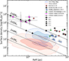 |
Fig. 5. Stellar mass surface density (Σmass) and effective radii (Reff) of the star clusters discussed in this work (magenta symbols), along with the following collection of gravitationally lensed star clusters from literature: Sunburst arc (Vanzella et al. 2022), Sunrise arc (Vanzella et al. 2023), Cosmic Archipelago (Messa et al. 2025), and Firefly Sparkle (Mowla et al. 2024). A comparison with local YMCs from Brown & Gnedin 2021 (red contours) and Milky Way globular clusters (Baumgardt & Hilker 2018, blue contours) shows the high surface densities in high-z clusters when compared to local ones (see also the dotted lines marking the constant stellar mass tracks). For the Cosmic Gems clusters, the black symbols refer to the values published in Adamo et al. (2024) assuming zphot = 10.2. |
5.2. New cluster candidates in the tail of the Cosmic Gems
The tail regions of the Cosmic Gems arc are characterized by unsmooth emission. Figure 6 shows a rest-UV image obtained by stacking the F150W and F200W NIRCam bands and applying a two-pixel Gaussian smoothing to enhance the inhomogeneities. While some of these inhomogeneities can be due to noise fluctuation, we identify four compact regions, which we name F–I, detected at the 3–4σ level. These can be reliably considered compact regions of the Cosmic Gems, as they are observed in both mirrored images of the arc and are detected also in the long-wavelength (LW) filters (see the inset of Fig. 6). These identified peaks are observationally faint, making it impossible to robustly derive their sizes. If we assume they are unresolved sources, considering the tangential magnifications in the tail (in the range μtan ≃ 10 − 30 according to the fiducial glafic lens model), their compactness results in estimated upper limits on intrinsic radii ranging from 3 to 10 pc. A forward-modeling reconstruction of the arc (see next Section) also suggests that these regions should be smaller than ≲10 pc in radii; otherwise, they would have a smoother morphology in NIRCam observations. Their measured observed magnitudes are in the range mAB = 28.3 − 29.3 mag, corresponding to mAB = 32.0 − 33.0 mag when delensed. Accounting for the redshift of the galaxy, we thus find that the magnitudes of these additional candidate clusters range from MAB = −14.5 to MAB = −15.5 mag. Assuming their ages are similar to the ones of the clusters discussed in Section 5.1 (∼10 − 30 Myr), their intrinsic masses should be M★ ∼ (0.5 − 8.0)×106 M⊙. According to their mass and radius estimates, these faint sources could be further massive clusters formed in the Cosmic Gems. Deeper observations would be necessary to give more robust constraints on their properties. The cluster mass function in the Cosmic Gems is further discussed in V25.
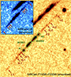 |
Fig. 6. Sum of the F150W and F200W NIRCam observations, smoothed by a two-pixel Gaussian kernel to better visualize the inhomogeneities along the arc. The clusters discussed in Adamo et al. (2024) and Section 5.1 of the current work are marked by green ellipses. The red arrows point to the position of the regions (detected at the 3 − 4σ level) discussed in the text. The same regions are also indicated in the inset panel, showing a smoothed version of the sum of the LW NIRCam filters available (F277W, F356W, F410M, and F444W). |
5.3. Forward modeling reconstruction of the arc
The reference glafic lens model was used to reconstruct the Cosmic Gems arc via a forward-modeling approach, based on the GravityFM software (Bergamini et al., in prep.). Sources with intrinsic sizes matching the values retrieved for the clusters (Table 1) were injected in the source plane, and their position and fluxes were chosen to match the observed NIRCam/F150W observations in the image plane (Fig. 7). In addition, an extended diffuse component was added to account for the diffuse light observed between the clusters (both in the case of NIRCam and of the NIRSpec). The exact origin of this diffuse light is unconstrained; here, we associated an emitting halo centered on cluster A with a radius of 65 parsec. Observational noise and the PSF effect were also accounted for, to ease the comparison with observations. Overall, this approach returns a good representation of the star clusters in the arc. We also notice that the forward modeling returns almost perfect mirrored images of the arc, while, in the case of observations, clusters C.2 and D.2 in the northwest image are blended, as already discussed by Adamo et al. (2024). This asymmetry is probably due to a small perturbation in the lens model, currently not accounted for. Sources with radii of 4 pc were inserted to account for the clumps F to I discussed in the previous section. The source-plane position of all the sources is shown in the bottom-right panels of Fig. 7. Clusters A to E occupy a small region, ∼50 pc in diameter, and B to E are found within ≲10 pc from each other. If also the regions in the tail are considered, the arc extends to a diameter up to ∼400 pc. To test the reliability of our method of delensing the observed radii into intrinsic values, we repeated the modeling assigning constant radii of 3 and 10 pc to all the clusters (top-right panels in Fig. 7). Already in the 3 pc case, clusters B–E became indistinguishable in the observations, with only cluster A remaining distinct, even if slightly elongated. In the 10 pc reconstruction, the arc becomes completely smooth in the central part. Assuming even larger intrinsic radii, the faint emissions in the tails (sources F–I) become undistinguishable from a smooth emission. This test provides further confirmation that, given our fiducial lens model, the compact appearance of the sources in the Cosmic Gems arc implies small intrinsic sizes (with Reff ≲ 1 pc).
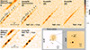 |
Fig. 7. Reconstruction of the Cosmic Gems arc in the image and source planes with the GravityFM tool (Bergamini et al., in prep.). Top panels, from left to right: Observed F150W image (I); the arc reproduced by inserting radii of the clusters in the source plane spanning the range 0.5 − 1.3 parsec (II, F150W PSF, with noise added); the same, with each assuming radii of 3 parsec (III); and the same, with each assuming radii of 10 parsec (IV). Bottom left panels: Same as in the top panels, but for NIRSpec data (V and VI, see text for more details). Bottom-right panels: Source plane reconstruction and the modeled sources inserted in the forward modeling reproducing the observed arc shown in panel II. |
6. Discussion
6.1. The post-burst phase in the star cluster regions
The analysis of the 1D spectra in Section 4 suggests that the regions corresponding to the position of the bright star clusters (BCDE and A) are in a post-burst phase, following a short (τ ∼ 2 Myr) star-formation episode around 10 − 20 Myr ago during which the star clusters formed. In order to test that the post-burst solution is not driven by the shape of the SFH assumed in Section 4, we refit the spectrum using the non-parametrized continuity SFH model by Leja et al. (2019), as implemented in Bagpipes. We considered age bins of 5 Myr in width in the range 0–30 Myr, and larger bins for older ages. We allowed sharp variations in star formation rate (SFR) between consecutive bins. The best-fit SFHs for the BCDE12 and A12 spectra (shown in Fig. 8) confirm that the regions are currently in a “dormant” phase after a burst started ∼15 Myr earlier lasting ∼5 − 10 Myr. The fit of A12 possibly suggests a slightly older burst (started ∼20 Myr ago) than in BCDE.
 |
Fig. 8. Comparison between the SFHs derived for the regions BCDE (left) and A (right) by assuming a parametric-delayed τ-model (black lines) and the nonparametric continuity model by Leja et al. (2019) (red curve). The SFR values are not rescaled to account for lensing. |
A possible alternative solution to the post-burst scenario is a younger SF region where the dearth of strong emission lines is due to a nonzero escape fraction (as also discussed in other studies of high-z quenched galaxy candidates, for example, Looser et al. 2024; Baker et al. 2025). Steep (β ≤ −2.5), such as those observed in all regions of the Cosmic Gems, are considered indirect tracers of fesc ≳ 0.1 (e.g., Chisholm et al. 2022; Flury et al. 2022a,b; Mascia et al. 2024, 2023; Topping et al. 2024). The main argument against this possibility is the presence of strong Lyα damping wings in the observed spectrum. This feature indicates large column densities of H I 1.2ex in the vicinity of the star clusters, as discussed in detail by Christensen et al., (in prep.), and thus a high gas opacity that would prevent the escape of ionizing radiation along the line of sight. However, it is worth noting that simulations suggest Lyman continuum leakage (if any) could still occur along transverse directions, which are not probed by our observations (He et al. 2020). Another point weakening the optically thin scenario is the fact that the UV slope remains relatively steep along the entire arc. While this would imply an exceptionally large, spatially resolved, optically thin region of the interstellar medium (ISM) spanning dozens of parsecs, the more likely explanation is that the galaxy is in a post-burst phase, during which the stellar populations can naturally produce relatively steep UV slopes and weak optical emission lines without invoking substantial leakage of ionizing photons. On the other hand, it is also plausible that in the past, during its bursty phase, the Cosmic Gems galaxy may have experienced a period when copious ionizing photons were able to escape (e.g., V25; Ferrara et al. 2025a).
The Cosmic Gems is thus the highest-redshift system observed in a post-starburst phase. Galaxies with similar properties (weak or absent emission lines and the presence of a Balmer break) have been recently observed up to z ∼ 7 − 9.5 and are thought to represent the temporarily “dormant” (or mini-quenched) phase of galaxies characterized by a bursty SFH (e.g., Looser et al. 2024; Baker et al. 2025; Tang et al. 2025). The Cosmic Gems provides also the opportunity to look at the small sub-galactic scales of a post-burst system, revealing the presence of dense (ΣM ∼ 105 − 106 M⊙ pc−2) and massive (M ∼ 106 M⊙) stellar clusters, as presented in Section 5.1. Those clusters are likely the main contributors to the observed spectra in this region.
We argue that their feedback (radiative or from supernovae, or both) may be the cause of the suppression of star formation in the region. This is expected from high-resolution cosmological simulations of systems that include young star clusters, which are formed in short bursts immediately followed by extended periods of quiescence or low-intensity activity (Calura et al. 2025; Pascale et al. 2025). Moreover, we know from local galaxies’ studies that stellar feedback from clusters clears their natal clouds, creating cavities in the gas, and in general regulating the star-formation process in their surroundings (see, e.g., Krumholz 2014; Chevance et al. 2020, for reviews). In starburst and in dwarf galaxies, stellar feedback can affect scales up to the entire host (e.g., Strickland & Heckman 2009; Bik et al. 2015). Strong radiation-driven feedback, temporarily pushing the gas and dust away from the galaxy, is one of the mechanisms that could explain the massive star-forming galaxies (sometimes referred to as “blue monsters”) observed at high-z, for example, in the “attenuation-free” scenario (Ferrara et al. 2025a,b). As mentioned above, the study of Christensen et al. (in prep.) suggests a large column density of gas aligned to the position of the clusters, thus implying that the galaxy is not devoid of gas and dust. The possibility that the Cosmic Gems galaxy was a “blue monster” in its recent past is discussed in V25. Finally, at high redshifts, the UV background could cause the suppression of star formation (Efstathiou 1992), especially in low-mass galaxies (105 − 107 M⊙, e.g., Katz et al. 2020). Given the mass of the Cosmic Gems (> 107 M⊙, Bradley et al. 2025; V25) and a redshift well before the end of the reionization (implying a limited UV background), we argue that it is not a main contribution to the SF suppression. Also, in this case, the large gas column density measured in Christensen et al., (in prep.) favors an “internal” quenching scenario, also in agreement with high-resolution simulations of star cluster formation at z > 8 (Calura et al. 2022, 2025; Garcia et al. 2023, 2025; Sugimura et al. 2024).
6.2. Sub-galactic spatial variation of the SFH?
The best-fit results from the CC and TAIL regions return longer SF episodes than for the cluster regions, thus with large uncertainties on most of the fitted properties. We already discussed how the emission lines from the CC spectrum may be powered by the rest-UV sources in the BCDE region, given their proximity in the source plane. A long SFH also seems inappropriate for an intrinsically small region such as CC (≲1 pc using the reference magnification from Appendix D).
On the other hand, the tail region includes a large but observationally UV faint area of the galaxy. The main spectroscopic features of its spectrum, discussed in the previous sections (see the top half of Appendix D) are poorly constrained yet consistent with those found in the other regions; i.e., neither the emission lines nor the Balmer break is detected, but their upper limits are larger than the detections in BCDE and hence do not exclude their presence. The main difference among regions is the extremely steep slope seen in the tail (β = −2.74 ± 0.06). We argue that the differences in the spectral fitting results may be due to the low signal and lack of spectral features in the tail. To further test the robustness of the results, we ran a fit with the continuity SFH assumption, as for the BCDE and A regions (Fig. 9). The fit returns unconstrained SFHs. We find that the spectrum is well fit by a young burst, as in the cluster regions, and by a longer SF event10 (as found with the delayed SFH parametrization in Section 4).
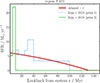 |
Fig. 9. Comparison between the SFHs obtained via the Bagpipes fitting of the spectrum in the TAIL, in the case of a parametric-delayed τ model (red curve) and of two realizations of the continuity Leja et al. (2019) model, assuming different priors (dotted-blue and solid green curves). The only difference between the priors used in the continuity model is the width of the distribution of the ΔSFR parameter, which regulates the difference in SFR between consecutive age bins; a small width produces the blue curve, while a large width, allowing bursty SF episodes, produces the green one. |
7. Conclusions
We reported the observation and analysis of JWST/NIRSpec prism IFU data (Program 5917, PI Vanzella) targeting the currently highest-redshift, strongly magnified (μ > 50) Cosmic Gems arc at z ≃ 10. The data cube covers the spectral range 0.8–5.3 μm, with a spectral resolution varying from R ∼ 30 to R ∼ 320. Additionally, VLT/MUSE spectroscopic redshifts of newly identified multiple images (Program 0112.A-2069(A), PI Bauer) were presented and incorporated to update the lens models. The improved models, developed using both Lenstool and Glafic, account for the CC intersecting the arc and are constrained by 54 multiple images from 18 sources spanning the redshift interval 1 < z < 10. The derived magnifications along the Cosmic Gems arc remain consistent with previous estimates, showing a steep gradient from μ ∼ 50 to μ ∼ 320 across the star clusters (A–E). These refined lens models enable a robust inference of the intrinsic properties of the subcomponents of the Cosmic Gems galaxy.
The key region of the arc is fully covered and spatially resolved in the NIRSpec IFU pointing. Our main results are summarized as follows:
-
(1)
The redshift of the Cosmic Gems is confirmed at z = 9.625 ± 0.002 from a high signal-to-noise integrated spectrum (S/N ≃ 40–100), which exhibits a prominent Lyα (damping wing) break, a very blue ultraviolet slope (βUV ranging from −2.5 to −2.7), a tentative Balmer break, and clear but relatively weak Hβ and [O III] λ4959 emission lines (with EWs of ≤38 Å and ≤75 Å, respectively, in the subregions where the lines are detected).
-
(2)
The spectral fitting of the subregions, encompassing both individual star clusters (e.g., A) and unresolved associations of clusters (BCDE), confirms the physical properties previously derived from imaging alone (Adamo et al. 2024). NIRCam-based SED fitting was updated to reflect the spectroscopic redshift (Section 5.1). In combination with spectral fitting (Section 4) and revised magnification maps (Section 3), the five clusters hosted within the Cosmic Gems arc (A, B, C, D, and E) exhibit radii in the range of 0.4–1.7 pc and stellar surface densities of ∼105 M⊙ pc−2. Four additional compact regions are identified along the extended tail of the arc, each with sizes ≲10 pc. Forward modeling reproduces the observed image-plane morphology and reveals that in the source plane the five star clusters are confined to a region ∼50 pc in extent, with four of them (B, C, D, and E) likely residing within a common ∼10 pc region. The entire arc spans an intrinsic area of radius ∼400 pc.
-
(3)
The nature of the Cosmic Gems galaxy suggests it is in a post-burst or dormant phase, representing an example of a z ∼ 10 weak emitter, a class of galaxies requiring further investigation through deep spectroscopy and/or lensing studies. Stellar feedback from the observed dense star clusters could be the main reason for the (temporary) quenching of the SF in the Cosmic Gems.
-
(4)
A compact and spatially unresolved Hβ and [O III] λ4959 emission component is detected near the CC, indicating that the emitting region is intrinsically small, with a size ≲0.9 pc (for μ > 500). This feature may arise from photoionization by a nearby star cluster (within a few parsecs) or from in situ star formation in a tiny H II region. Although the emitting region is extremely compact, its inferred physical properties remain preliminary, limited by a low S/N and the absence of a detectable NIRCam counterpart. Given the large magnification, the contribution of the CC region to the total arc emission is negligible.
Acknowledgments
This work is based on observations made with the NASA/ESA/CSA James Webb Space Telescope (JWST) and Hubble Space Telescope (HST). These observations are associated with JWST GO program n.4212 (PI L. Bradley) and n.5917 (PI E. Vanzella). The data can be obtained from the Mikulski Archive for Space Telescopes at the Space Telescope Science Institute, which is operated by the Association of Universities for Research in Astronomy, Inc., under NASA contract NAS 5-03127 for JWST. We thank the anonymous referee for helping improving the manuscript. MM, EV and FC acknowledge financial support through grants PRIN-MIUR 2020SKSTHZ, the INAF GO Grant 2022 “The revolution is around the corner: JWST will probe globular cluster precursors and Population III stellar clusters at cosmic dawn” and INAF GO Grant 2024 “Mapping Star Cluster Feedback in a Galaxy 450 Myr after the Big Bang”, and by the European Union – NextGenerationEU within PRIN 2022 project n.20229YBSAN – Globular clusters in cosmological simulations and lensed fields: from their birth to the present epoch. This work was supported by JSPS KAKENHI Grant Numbers JP25H00662, JP22K21349. AA acknowledges support by the Swedish research council Vetenskapsrådet (VR 2021-05559, and VR consolidator grant 2024-02061). FEB acknowledges support from ANID-Chile BASAL CATA FB210003, FONDECYT Regular 1241005, and Millennium Science Initiative, AIM23-0001. MB acknowledges support from the Slovenian national research agency ARRS through grant N1-0238. EZ acknowledges project grant 2022-03804 from the Swedish Research Council. R.A.W., S.H.C., and R.A.J. acknowledge support from NASA JWST Interdisciplinary Scientist grants NAG5-12460, NNX14AN10G and 80NSSC18K0200 from GSFC. AZ acknowledges support by grant 2020750 from the United States-Israel Binational Science Foundation (BSF) and grant 2109066 from the United States National Science Foundation (NSF), and by the Israel Science Foundation Grant No. 864/23.
References
- Adamo, A., Bradley, L. D., Vanzella, E., et al. 2024, Nature, 632, 513 [NASA ADS] [CrossRef] [Google Scholar]
- Arrabal Haro, P., Dickinson, M., Finkelstein, S. L., et al. 2023, ApJ, 951, L22 [NASA ADS] [CrossRef] [Google Scholar]
- Atek, H., Shuntov, M., Furtak, L. J., et al. 2023, MNRAS, 519, 1201 [Google Scholar]
- Atek, H., Labbé, I., Furtak, L. J., et al. 2024, Nature, 626, 975 [NASA ADS] [CrossRef] [Google Scholar]
- Baker, W. M., D’Eugenio, F., Maiolino, R., et al. 2025, A&A, 697, A90 [NASA ADS] [CrossRef] [EDP Sciences] [Google Scholar]
- Baumgardt, H., & Hilker, M. 2018, MNRAS, 478, 1520 [Google Scholar]
- Bik, A., Östlin, G., Hayes, M., et al. 2015, A&A, 576, L13 [NASA ADS] [CrossRef] [EDP Sciences] [Google Scholar]
- Binggeli, C., Zackrisson, E., Ma, X., et al. 2019, MNRAS, 489, 3827 [Google Scholar]
- Bradley, L. D., Adamo, A., Vanzella, E., et al. 2025, ApJ, 991, 32 [Google Scholar]
- Brammer, G. B., van Dokkum, P. G., & Coppi, P. 2008, ApJ, 686, 1503 [Google Scholar]
- Brown, G., & Gnedin, O. Y. 2021, MNRAS, 508, 5935 [NASA ADS] [CrossRef] [Google Scholar]
- Bunker, A. J., Saxena, A., Cameron, A. J., et al. 2023, A&A, 677, A88 [NASA ADS] [CrossRef] [EDP Sciences] [Google Scholar]
- Bushouse, H., Eisenhamer, J., Dencheva, N., et al. 2023, https://doi.org/10.5281/zenodo.7577320 [Google Scholar]
- Calura, F., Lupi, A., Rosdahl, J., et al. 2022, MNRAS, 516, 5914 [Google Scholar]
- Calura, F., Pascale, R., Agertz, O., et al. 2025, A&A, 698, A207 [NASA ADS] [CrossRef] [EDP Sciences] [Google Scholar]
- Calzetti, D., Armus, L., Bohlin, R. C., et al. 2000, ApJ, 533, 682 [NASA ADS] [CrossRef] [Google Scholar]
- Carnall, A. C., McLure, R. J., Dunlop, J. S., & Davé, R. 2018, MNRAS, 480, 4379 [Google Scholar]
- Carnall, A. C., McLure, R. J., Dunlop, J. S., et al. 2019, MNRAS, 490, 417 [Google Scholar]
- Carniani, S., Hainline, K., D’Eugenio, F., et al. 2024, Nature, 633, 318 [CrossRef] [Google Scholar]
- Carvajal-Bohorquez, C., Ciesla, L., Laporte, N., et al. 2026, A&A, 704, A290 [Google Scholar]
- Castellano, M., Napolitano, L., Fontana, A., et al. 2024, ApJ, 972, 143 [Google Scholar]
- Chevance, M., Kruijssen, J. M. D., Vazquez-Semadeni, E., et al. 2020, Space Sci. Rev., 216, 50 [NASA ADS] [CrossRef] [Google Scholar]
- Chisholm, J., Saldana-Lopez, A., Flury, S., et al. 2022, MNRAS, 517, 5104 [CrossRef] [Google Scholar]
- Choi, J., Conroy, C., & Byler, N. 2017, ApJ, 838, 159 [NASA ADS] [CrossRef] [Google Scholar]
- Covelo-Paz, A., Meuwly, C., Oesch, P. A., et al. 2025, A&A, accepted [arXiv:2506.22540] [Google Scholar]
- Cullen, F., McLure, R. J., McLeod, D. J., et al. 2023, MNRAS, 520, 14 [NASA ADS] [CrossRef] [Google Scholar]
- Curtis-Lake, E., Carniani, S., Cameron, A., et al. 2023, Nat. Astron., 7, 622 [NASA ADS] [CrossRef] [Google Scholar]
- Dekel, A., Sarkar, K. C., Birnboim, Y., Mandelker, N., & Li, Z. 2023, MNRAS, 523, 3201 [NASA ADS] [CrossRef] [Google Scholar]
- Dome, T., Tacchella, S., Fialkov, A., et al. 2024, MNRAS, 527, 2139 [Google Scholar]
- Donnan, C. T., Dickinson, M., Taylor, A. J., et al. 2025, ApJ, 993, 224 [Google Scholar]
- Efstathiou, G. 1992, MNRAS, 256, 43P [Google Scholar]
- Eldridge, J. J., Stanway, E. R., Xiao, L., et al. 2017, PASA, 34, e058 [Google Scholar]
- Endsley, R., Stark, D. P., Whitler, L., et al. 2024, MNRAS, 533, 1111 [NASA ADS] [CrossRef] [Google Scholar]
- Endsley, R., Chisholm, J., Stark, D. P., Topping, M. W., & Whitler, L. 2025, ApJ, 987, 189 [Google Scholar]
- Faucher-Giguère, C.-A. 2018, MNRAS, 473, 3717 [Google Scholar]
- Ferrara, A., Pallottini, A., & Dayal, P. 2023, MNRAS, 522, 3986 [NASA ADS] [CrossRef] [Google Scholar]
- Ferrara, A., Pallottini, A., & Sommovigo, L. 2025a, A&A, 694, A286 [NASA ADS] [CrossRef] [EDP Sciences] [Google Scholar]
- Ferrara, A., Carniani, S., di Mascia, F., et al. 2025b, A&A, 694, A215 [NASA ADS] [CrossRef] [EDP Sciences] [Google Scholar]
- Finkelstein, S. L., Leung, G. C. K., Bagley, M. B., et al. 2024, ApJ, 969, L2 [NASA ADS] [CrossRef] [Google Scholar]
- Flury, S. R., Jaskot, A. E., Ferguson, H. C., et al. 2022a, ApJS, 260, 1 [NASA ADS] [CrossRef] [Google Scholar]
- Flury, S. R., Jaskot, A. E., Ferguson, H. C., et al. 2022b, ApJ, 930, 126 [NASA ADS] [CrossRef] [Google Scholar]
- Fujimoto, S., Arrabal Haro, P., Dickinson, M., et al. 2023, ApJ, 949, L25 [NASA ADS] [CrossRef] [Google Scholar]
- Fujimoto, S., Wang, B., Weaver, J. R., et al. 2024, ApJ, 977, 250 [NASA ADS] [CrossRef] [Google Scholar]
- Gaia Collaboration (Brown, A. G. A., et al.) 2018, A&A, 616, A1 [NASA ADS] [CrossRef] [EDP Sciences] [Google Scholar]
- Garcia, F. A. B., Ricotti, M., Sugimura, K., & Park, J. 2023, MNRAS, 522, 2495 [NASA ADS] [CrossRef] [Google Scholar]
- Garcia, F. A. B., Ricotti, M., & Sugimura, K. 2025, Open J. Astrophys., 8, 146 [Google Scholar]
- Gelli, V., Salvadori, S., Ferrara, A., Pallottini, A., & Carniani, S. 2023, ApJ, 954, L11 [NASA ADS] [CrossRef] [Google Scholar]
- Gladders, M. D., & Yee, H. K. C. 2000, AJ, 120, 2148 [NASA ADS] [CrossRef] [Google Scholar]
- Hainline, K. N., D’Eugenio, F., Jakobsen, P., et al. 2024, ApJ, 976, 160 [NASA ADS] [CrossRef] [Google Scholar]
- He, C.-C., Ricotti, M., & Geen, S. 2020, MNRAS, 492, 4858 [Google Scholar]
- Heintz, K. E., Brammer, G. B., Watson, D., et al. 2025, A&A, 693, A60 [Google Scholar]
- Helton, J. M., Rieke, G. H., Alberts, S., et al. 2025, Nat. Astron., 9, 729 [Google Scholar]
- Hsiao, T. Y.-Y., Abdurro’uf, Coe, D., et al. 2024, ApJ, 973, 8 [NASA ADS] [CrossRef] [Google Scholar]
- Hutter, A., Cueto, E. R., Dayal, P., et al. 2025, A&A, 694, A254 [NASA ADS] [CrossRef] [EDP Sciences] [Google Scholar]
- Inoue, A. K., Shimizu, I., Iwata, I., & Tanaka, M. 2014, MNRAS, 442, 1805 [NASA ADS] [CrossRef] [Google Scholar]
- Jullo, E., Kneib, J. P., Limousin, M., et al. 2007, New J. Phys., 9, 447 [Google Scholar]
- Katz, H., Ramsoy, M., Rosdahl, J., et al. 2020, MNRAS, 494, 2200 [NASA ADS] [CrossRef] [Google Scholar]
- Kawamata, R., Oguri, M., Ishigaki, M., Shimasaku, K., & Ouchi, M. 2016, ApJ, 819, 114 [NASA ADS] [CrossRef] [Google Scholar]
- Kroupa, P. 2001, MNRAS, 322, 231 [NASA ADS] [CrossRef] [Google Scholar]
- Krumholz, M. R. 2014, Phys. Rep., 539, 49 [Google Scholar]
- Leja, J., Carnall, A. C., Johnson, B. D., Conroy, C., & Speagle, J. S. 2019, ApJ, 876, 3 [Google Scholar]
- Li, Z., Dekel, A., Sarkar, K. C., et al. 2024, A&A, 690, A108 [NASA ADS] [CrossRef] [EDP Sciences] [Google Scholar]
- Looser, T. J., D’Eugenio, F., Maiolino, R., et al. 2024, Nature, 629, 53 [Google Scholar]
- Looser, T. J., D’Eugenio, F., Maiolino, R., et al. 2025, A&A, 697, A88 [NASA ADS] [CrossRef] [EDP Sciences] [Google Scholar]
- Mascia, S., Pentericci, L., Calabrò, A., et al. 2023, A&A, 672, A155 [NASA ADS] [CrossRef] [EDP Sciences] [Google Scholar]
- Mascia, S., Pentericci, L., Calabrò, A., et al. 2024, A&A, 685, A3 [NASA ADS] [CrossRef] [EDP Sciences] [Google Scholar]
- Mason, C. A., Trenti, M., & Treu, T. 2023, MNRAS, 521, 497 [NASA ADS] [CrossRef] [Google Scholar]
- Messa, M., Vanzella, E., Loiacono, F., et al. 2025, A&A, 694, A59 [NASA ADS] [CrossRef] [EDP Sciences] [Google Scholar]
- Mowla, L., Iyer, K., Asada, Y., et al. 2024, Nature, 636, 332 [Google Scholar]
- Naidu, R. P., Oesch, P. A., van Dokkum, P., et al. 2022, ApJ, 940, L14 [NASA ADS] [CrossRef] [Google Scholar]
- Naidu, R. P., Oesch, P. A., Brammer, G., et al. 2025, ArXiv e-prints [arXiv:2505.11263] [Google Scholar]
- Nakajima, K., Ouchi, M., Xu, Y., et al. 2022, ApJS, 262, 3 [CrossRef] [Google Scholar]
- Napolitano, L., Castellano, M., Pentericci, L., et al. 2025, A&A, 693, A50 [NASA ADS] [CrossRef] [EDP Sciences] [Google Scholar]
- Navarro, J. F., Frenk, C. S., & White, S. D. M. 1997, ApJ, 490, 493 [Google Scholar]
- Oguri, M. 2010, PASJ, 62, 1017 [NASA ADS] [Google Scholar]
- Oguri, M. 2021, PASP, 133, 074504 [NASA ADS] [CrossRef] [Google Scholar]
- Pallottini, A., & Ferrara, A. 2023, A&A, 677, L4 [NASA ADS] [CrossRef] [EDP Sciences] [Google Scholar]
- Pascale, R., Calura, F., Vesperini, E., et al. 2025, A&A, 699, A31 [NASA ADS] [CrossRef] [EDP Sciences] [Google Scholar]
- Paterno-Mahler, R., Sharon, K., Coe, D., et al. 2018, ApJ, 863, 154 [Google Scholar]
- Piqueras, L., Conseil, S., Shepherd, M., et al. 2019, ASP Conf. Ser., 521, 545 [Google Scholar]
- Richard, J., Claeyssens, A., Lagattuta, D., et al. 2021, A&A, 646, A83 [EDP Sciences] [Google Scholar]
- Roberts-Borsani, G., Treu, T., Chen, W., et al. 2023, Nature, 618, 480 [NASA ADS] [CrossRef] [Google Scholar]
- Robertson, B. E., Tacchella, S., Johnson, B. D., et al. 2023, Nat. Astron., 7, 611 [NASA ADS] [CrossRef] [Google Scholar]
- Robertson, B., Johnson, B. D., Tacchella, S., et al. 2024, ApJ, 970, 31 [NASA ADS] [CrossRef] [Google Scholar]
- Salmon, B., Coe, D., Bradley, L., et al. 2018, ApJ, 864, L22 [Google Scholar]
- Sanders, R. L., Shapley, A. E., Topping, M. W., Reddy, N. A., & Brammer, G. B. 2024, ApJ, 962, 24 [NASA ADS] [CrossRef] [Google Scholar]
- Sanders, R. L., Shapley, A. E., Topping, M. W., et al. 2025, ApJ, submitted [arXiv:2508.10099] [Google Scholar]
- Sharon, K., Bayliss, M. B., Dahle, H., et al. 2020, ApJS, 247, 12 [CrossRef] [Google Scholar]
- Somerville, R. S., Yung, L. Y. A., Lancaster, L., et al. 2025, MNRAS, 544, 3774 [Google Scholar]
- Stanway, E. R., & Eldridge, J. J. 2018, MNRAS, 479, 75 [NASA ADS] [CrossRef] [Google Scholar]
- Stasińska, G., & Leitherer, C. 1996, ApJS, 107, 661 [Google Scholar]
- Strait, V., Bradač, M., Coe, D., et al. 2020, ApJ, 888, 124 [NASA ADS] [CrossRef] [Google Scholar]
- Strickland, D. K., & Heckman, T. M. 2009, ApJ, 697, 2030 [Google Scholar]
- Sugimura, K., Ricotti, M., Park, J., Garcia, F. A. B., & Yajima, H. 2024, ApJ, 970, 14 [NASA ADS] [CrossRef] [Google Scholar]
- Sun, G., Faucher-Giguère, C.-A., Hayward, C. C., et al. 2023a, ApJ, 955, L35 [CrossRef] [Google Scholar]
- Sun, G., Faucher-Giguère, C.-A., Hayward, C. C., & Shen, X. 2023b, MNRAS, 526, 2665 [NASA ADS] [CrossRef] [Google Scholar]
- Tacchella, S., Dekel, A., Carollo, C. M., et al. 2016, MNRAS, 457, 2790 [Google Scholar]
- Tacchella, S., Forbes, J. C., & Caplar, N. 2020, MNRAS, 497, 698 [Google Scholar]
- Tacchella, S., Eisenstein, D. J., Hainline, K., et al. 2023, ApJ, 952, 74 [NASA ADS] [CrossRef] [Google Scholar]
- Tang, M., Stark, D. P., Mason, C. A., et al. 2025, ApJ, submitted [arXiv:2507.08245] [Google Scholar]
- Topping, M. W., Stark, D. P., Endsley, R., et al. 2024, MNRAS, 529, 4087 [NASA ADS] [CrossRef] [Google Scholar]
- Trinca, A., Schneider, R., Valiante, R., et al. 2024, MNRAS, 529, 3563 [NASA ADS] [CrossRef] [Google Scholar]
- Vanzella, E., Castellano, M., Bergamini, P., et al. 2022, A&A, 659, A2 [NASA ADS] [CrossRef] [EDP Sciences] [Google Scholar]
- Vanzella, E., Claeyssens, A., Welch, B., et al. 2023, ApJ, 945, 53 [NASA ADS] [CrossRef] [Google Scholar]
- Vanzella, E., Loiacono, F., Messa, M., et al. 2024, A&A, 691, A251 [NASA ADS] [CrossRef] [EDP Sciences] [Google Scholar]
- Vanzella, E., Messa, M., Adamo, A., et al. 2026, A&A, in press https://doi.org/10.1051/0004-6361/202556570 [Google Scholar]
- Wang, B., Fujimoto, S., Labbé, I., et al. 2023, ApJ, 957, L34 [NASA ADS] [CrossRef] [Google Scholar]
- Weilbacher, P. M., Palsa, R., Streicher, O., et al. 2020, A&A, 641, A28 [NASA ADS] [CrossRef] [EDP Sciences] [Google Scholar]
- Welch, B., Coe, D., Zitrin, A., et al. 2023, ApJ, 943, 2 [Google Scholar]
- Whitler, L., Stark, D. P., Topping, M. W., et al. 2025, ApJ, 992, 63 [Google Scholar]
- Zavala, J. A., Castellano, M., Akins, H. B., et al. 2025, Nat. Astron., 9, 155 [Google Scholar]
The kernels are produced assuming Gaussian profiles for the PSF. The PSF-correction overall is performed using the DPUSER interactive language, https://www.mpe.mpg.de/~ott/dpuser/
The redshift difference Δz = 0.005 converts into Δv = 140 km s−1, while the resolving power of the prism at ∼5 μm (R ∼ 300) corresponds to Δv(R) = 1000 km s−1.
The same prescription is used also in the Bagpipes code used to fit the spectra in the current work. See Section 4.2.
The flux of the [O III] λ5007 line is derived assuming again λ5007/λ4959 = 2.98.
This value is the average of the magnifications extracted for BCDE1 and BCDE2 in the Appendix B.
Only a fraction of the tail of the arc is observed with the IFU in the southeast region. In order to have a complete view of the region we only considered the northwest image.
This calculation assumes a conservative magnification of μ = 320, corresponding to the magnification at the position of cluster E (see Appendix B).
This methodology considers each pixel independently and therefore does not account for the PSF spreading the flux of compact regions over several pixels.
The difference in the two recovered SFHs is caused by different prior assumptions, namely the width of the student-t distribution used as prior for ΔSFR, which describes the variation of SFR between consecutive time bins.
Appendix A: Additional plots on data reduction and PSF-matching of the cube
In this appendix we provide additional material about the data reduction process. Fig. A.1 shows the cube spaxels used to estimate the background, by fitting a 2D polynomial in each wavelength slice. As mentioned in the main text, the background-subtracted cubes produced with polynomial fits of zeroth to second order are almost indistinguishable.
The comparison between one spectrum coming from stage 3 of the official pipeline, reduced at 100 mas scale, and two spectra from our customized pipeline (at 50 and 100 mas), all taken from the same region, is presented in Fig. A.2.
Finally, Fig. A.3 shows the relation used to PSF-match the cube across wavelengths. This reference curve (purple line in the figure) comes from the FWHM of the PSFs produced by the STPSF tool. For comparison, we estimate the FWHM in the transversal direction of the arc of the BCDE1 clump in our data (green data in the figure). To increase the signal of this source, stackings of 30 slices are created along the wavelength range; all fits are performed assuming a 2D ellipse Gaussian model, and fixing the position angle to the direction of the arc. The assumption behind this test is that the source is spatially unresolved in NIRSpec-IFU, as supported by its appearance in NIRCam imaging. The wavelength trend recovered in this way (shown in Fig. A.3) is overall consistent with the reference one.
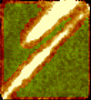 |
Fig. A.1. Green spaxels used for background estimation. The underlying map, produced by collapsing all the slices, is used to show the position of the target arc at z = 9.625 and the position of a lower-redshift galaxy (z = 2.531) within the field of view. |
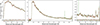 |
Fig. A.2. Comparison of the reference reduction (customized, at 50 mas, black curve) with the reduction at 100 mas (red curve) and the standard pipeline reduction (green curve). All spectra were extracted from the same region (BCDE12_CC, shown in the main text in Fig. 1). Central panel: Full spectrum. Lateral panels: Insets in the range of the Lyα drop (left) and of the emission lines (right). The difference between the reference and the other reductions is compared to the uncertainties. |
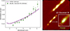 |
Fig. A.3. Variation of the PSF across wavelengths in the cube (purple line) used to create a PSF-matched final cube. The line was estimated from the FWHM of a series of PSFs created by STPSF. The green points, used for comparison, show estimates of the FWHM at various wavelengths on the minor (unresolved) axis of source BCDE1 (as shown in the right panel). |
Appendix B: Multiple images, lens model comparison, and magnification map
A comparison of the magnifications, derived at the position of the star clusters, by the glafic and Lenstool lens models (see Section 3) is given in Tab.B.1. On average Lenstool predicts larger magnification values, by a factor of up to 1.5.
Multiple images used for the strong lens mass modeling are summarized in Tab. B.2. Two systems lack reliable redshift (photometric or spectroscopic), which is thus left as a free parameter in the fit. The magnification map at z = 9.625 in the region occupied by the Cosmic Gems arc is shown in Fig. B.1, together with the apertures used to extract the amplification values assigned to the star clusters and to the NIRSpec masks defined in the main text. These apertures (solid circles and ellipses) are centered at the sources’ observed positions; in the case of star clusters A.1, A.2, B.1 and B.2 we also show the predicted positions from the lens model (dotted white circles) that, by construction, are very close to the observed ones. Fig. B.1 also shows the distribution of amplification values obtained by considering the 100 MCMC extractions of the lens model (see Section. 3 for details); the median magnification is considered as "reference" for each region. When mirrored regions are considered together (i.e., BCDE1,2 in Appendix D), the final magnification is the average of the two.
Star cluster magnifications in different lens models.
Multiple images used for strong lens mass modeling.
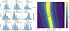 |
Fig. B.1. MCMC extractions from 100 magnification maps produced with glafic as described in Section 3. Left: Histograms, medians, and 16-84% percentiles of the magnifications for the relevant regions of the Cosmic Gems arc discussed in this work. Right: Color-coded total magnification map indicating regions within which the magnifications were calculated (by computing the median of the values within the aperture). The regions correspond to the observed positions of the entries discussed in this work. As a comparison, the dotted white circles mark the model positions of the regions used among the constraints of the model. By construction, the observed and model positions are very close to each other. |
Appendix C: Spectra from all mask apertures
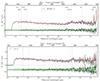 |
Fig. C.1. 1D observed and best-fit spectra (gray and red curves, respectively) for the main mask apertures discussed in the main text (Section 4). The residuals between the observed and best-model spectra are shown as a black curve, while the green band encloses the ± 1σ uncertainties from the observations. Both the residuals and uncertainties are, in some cases, shifted arbitrarily to avoid confusion with the observed spectra. We note that the fit is performed only for (observed) wavelengths longer than 1.7 μm. The expected wavelengths of the main UV and optical lines are shown. |
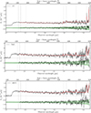 |
Fig. C.1. Continued. |
Appendix D: Table of spectral properties
Main spectroscopic properties of the Cosmic Gems arc and its subregions.
Appendix E: BC and DE subregions
In order to test possible small-scale variations within the BCDE1,2 region, we divide the mask aperture in two (BC1,2 and DE1,2, see Fig. E.1). We remind that given the large PSF of the NIRSpec/IFU, compared to NIRCam, the emission within BCDE1,2 is spatially only marginally resolved (see Fig. 1). The two spectra show very similar βUV ≈ −2.5 and Balmer break (≈1.2−1.3), with DE1,2 having slightly larger EWs than BC1,2. The direct comparison of the two spectra is shown in Fig. E.1. The best-fit from Bagpipes are also overall consistent among the two subregions, returning young ages (9 − 14 Myr) and a short burst (τ = 2−3 Myr). Given the large difference in magnification between the two subregions (μBC1,2 = 107 vs. μDE1,2 = 225), the intrinsic mass in the BC region, dominates the mass budget of the BCDE region. The total mass coming from the two fits remains consistent with the mass of BCDE1,2 estimated in Section 4.
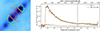 |
Fig. E.1. (Left): Division of the BCDE1 and BCDE2 mask apertures into the sub-apertures BC1-DE1 and BC2-DE2. (Right): Comparison of the 1D spectra extracted from the BC1,2 and DE1,2 mask apertures. The latter were rescaled (by a factor of 1.39) in order to match the average Fλ of BC1,2 in the observed wavelength range 3.7 to 3.8 μm. This interval was chosen to highlight possible differences between the spectra in the UV slope (blueward of 3.7 μm) or in the Balmer break amplitude (redward of 3.8 μm). |
All Tables
All Figures
|
Fig. 1. JWST/NIRSpec spectrum, NIRCam, and pseudo-NIRCam images (NIRSpec-IFU based) of the Cosmic Gems arc. Top: 1D NIRSpec prism spectrum (from the PSF-matched cube) extracted from the full arc (with its aperture mask shown in the bottom-central panel), showing the large Lyα-break and damping at ≃1.3 μm, along with two weak emission lines, Hβ and [O III] λ4959, on the rightmost side of the spectral range. A weak Balmer break is also detected (Section 4). The 1σ uncertainty spectrum is shown in red. The wavelengths corresponding to the main undetected UV and optical lines are shown with dashed lines. The throughputs of the NIRCam filters covering the field are shown in green, for reference. Bottom: From left to right, JWST/NIRCam stacked F150W + F200W image with the NIRSpec-IFU field of view outlined; collapsed NIRSpec IFU data cube in the rest-UV (covering the observed wavelength range of F150W and F200W), before (middle) and after (right) PSF-matching. The last panel also includes the outlines of the masks used to extract the 1D spectra for the regions discussed in the main text. |
| In the text | |
|
Fig. 2. JWST/NIRCam color image of the galaxy cluster SPT0615 field with the locations of the Cosmic Gems arc and its counter-image marked, along with the critical lines for the z = 9.625 lens models from LENSTOOL (red line) and glafic (green line). The yellow-shaded square marks the field of view of the JWST/NIRSpec IFU observations. |
| In the text | |
|
Fig. 3. Left: 2D map of the stacked Hβ + [O III] λ4959 in the wavelength range 5.15–5.3 μm (see text for more details). The red mask corresponds to the regions BCDE1,2 and CC (defined in Fig. 1), used to extract the spectrum on the right. The inset shows the NIRCam F150W + F200W data with overlaid black contours showing the peak of the Hβ + [O III] λ4959 emission and the CCs from GLAFIC (blue) and Lenstool (red). The white circle (in both the map and the inset) denote the FWHM of the NIRSpec-IFU PSF, while the NIRCam one is plotted as a black circle in the inset. Right: 1D spectrum (thick gray line) in the wavelength range of the detected emission lines. The continuum and line best-fitting result are shown as a red line. The error spectrum and spectral fit residuals are shown in green and light gray, respectively. The gray bands mark the portion of the spectrum not included in the fit. |
| In the text | |
|
Fig. 4. Spectrum of the combined BCDE12 regions (gray), along with the best-fit model (red), residuals (black), and ±1σ uncertainties (green). Bottom panels: Zoom-ins on the regions where the best-fit predicts the main emission lines. |
| In the text | |
|
Fig. 5. Stellar mass surface density (Σmass) and effective radii (Reff) of the star clusters discussed in this work (magenta symbols), along with the following collection of gravitationally lensed star clusters from literature: Sunburst arc (Vanzella et al. 2022), Sunrise arc (Vanzella et al. 2023), Cosmic Archipelago (Messa et al. 2025), and Firefly Sparkle (Mowla et al. 2024). A comparison with local YMCs from Brown & Gnedin 2021 (red contours) and Milky Way globular clusters (Baumgardt & Hilker 2018, blue contours) shows the high surface densities in high-z clusters when compared to local ones (see also the dotted lines marking the constant stellar mass tracks). For the Cosmic Gems clusters, the black symbols refer to the values published in Adamo et al. (2024) assuming zphot = 10.2. |
| In the text | |
|
Fig. 6. Sum of the F150W and F200W NIRCam observations, smoothed by a two-pixel Gaussian kernel to better visualize the inhomogeneities along the arc. The clusters discussed in Adamo et al. (2024) and Section 5.1 of the current work are marked by green ellipses. The red arrows point to the position of the regions (detected at the 3 − 4σ level) discussed in the text. The same regions are also indicated in the inset panel, showing a smoothed version of the sum of the LW NIRCam filters available (F277W, F356W, F410M, and F444W). |
| In the text | |
|
Fig. 7. Reconstruction of the Cosmic Gems arc in the image and source planes with the GravityFM tool (Bergamini et al., in prep.). Top panels, from left to right: Observed F150W image (I); the arc reproduced by inserting radii of the clusters in the source plane spanning the range 0.5 − 1.3 parsec (II, F150W PSF, with noise added); the same, with each assuming radii of 3 parsec (III); and the same, with each assuming radii of 10 parsec (IV). Bottom left panels: Same as in the top panels, but for NIRSpec data (V and VI, see text for more details). Bottom-right panels: Source plane reconstruction and the modeled sources inserted in the forward modeling reproducing the observed arc shown in panel II. |
| In the text | |
|
Fig. 8. Comparison between the SFHs derived for the regions BCDE (left) and A (right) by assuming a parametric-delayed τ-model (black lines) and the nonparametric continuity model by Leja et al. (2019) (red curve). The SFR values are not rescaled to account for lensing. |
| In the text | |
|
Fig. 9. Comparison between the SFHs obtained via the Bagpipes fitting of the spectrum in the TAIL, in the case of a parametric-delayed τ model (red curve) and of two realizations of the continuity Leja et al. (2019) model, assuming different priors (dotted-blue and solid green curves). The only difference between the priors used in the continuity model is the width of the distribution of the ΔSFR parameter, which regulates the difference in SFR between consecutive age bins; a small width produces the blue curve, while a large width, allowing bursty SF episodes, produces the green one. |
| In the text | |
|
Fig. A.1. Green spaxels used for background estimation. The underlying map, produced by collapsing all the slices, is used to show the position of the target arc at z = 9.625 and the position of a lower-redshift galaxy (z = 2.531) within the field of view. |
| In the text | |
|
Fig. A.2. Comparison of the reference reduction (customized, at 50 mas, black curve) with the reduction at 100 mas (red curve) and the standard pipeline reduction (green curve). All spectra were extracted from the same region (BCDE12_CC, shown in the main text in Fig. 1). Central panel: Full spectrum. Lateral panels: Insets in the range of the Lyα drop (left) and of the emission lines (right). The difference between the reference and the other reductions is compared to the uncertainties. |
| In the text | |
|
Fig. A.3. Variation of the PSF across wavelengths in the cube (purple line) used to create a PSF-matched final cube. The line was estimated from the FWHM of a series of PSFs created by STPSF. The green points, used for comparison, show estimates of the FWHM at various wavelengths on the minor (unresolved) axis of source BCDE1 (as shown in the right panel). |
| In the text | |
|
Fig. B.1. MCMC extractions from 100 magnification maps produced with glafic as described in Section 3. Left: Histograms, medians, and 16-84% percentiles of the magnifications for the relevant regions of the Cosmic Gems arc discussed in this work. Right: Color-coded total magnification map indicating regions within which the magnifications were calculated (by computing the median of the values within the aperture). The regions correspond to the observed positions of the entries discussed in this work. As a comparison, the dotted white circles mark the model positions of the regions used among the constraints of the model. By construction, the observed and model positions are very close to each other. |
| In the text | |
|
Fig. C.1. 1D observed and best-fit spectra (gray and red curves, respectively) for the main mask apertures discussed in the main text (Section 4). The residuals between the observed and best-model spectra are shown as a black curve, while the green band encloses the ± 1σ uncertainties from the observations. Both the residuals and uncertainties are, in some cases, shifted arbitrarily to avoid confusion with the observed spectra. We note that the fit is performed only for (observed) wavelengths longer than 1.7 μm. The expected wavelengths of the main UV and optical lines are shown. |
| In the text | |
|
Fig. C.1. Continued. |
| In the text | |
|
Fig. E.1. (Left): Division of the BCDE1 and BCDE2 mask apertures into the sub-apertures BC1-DE1 and BC2-DE2. (Right): Comparison of the 1D spectra extracted from the BC1,2 and DE1,2 mask apertures. The latter were rescaled (by a factor of 1.39) in order to match the average Fλ of BC1,2 in the observed wavelength range 3.7 to 3.8 μm. This interval was chosen to highlight possible differences between the spectra in the UV slope (blueward of 3.7 μm) or in the Balmer break amplitude (redward of 3.8 μm). |
| In the text | |
Current usage metrics show cumulative count of Article Views (full-text article views including HTML views, PDF and ePub downloads, according to the available data) and Abstracts Views on Vision4Press platform.
Data correspond to usage on the plateform after 2015. The current usage metrics is available 48-96 hours after online publication and is updated daily on week days.
Initial download of the metrics may take a while.