| Issue |
A&A
Volume 705, January 2026
|
|
|---|---|---|
| Article Number | A90 | |
| Number of page(s) | 11 | |
| Section | Extragalactic astronomy | |
| DOI | https://doi.org/10.1051/0004-6361/202556627 | |
| Published online | 09 January 2026 | |
A deep X-ray look to the most obscured quasar at z ∼ 3.6 and its environment
1
Dipartimento di Matematica e Fisica, Universitá degli Studi Roma Tre, Via della Vasca Navale 84, 00146 Roma, Italy
2
INAF – Osservatorio Astronomico di Roma, Via di Frascati 33, 00078 Monte Porzio Catone, Italy
3
INAF – Osservatorio Astrofisico di Arcetri, Largo E. Fermi 5, Firenze I-50125, Italy
4
Dipartimento di Fisica e Astronomia, Universitá degli Studi di Firenze, Via G. Sansone 1, 50019 Sesto Fiorentino, Italy
5
Max-Planck-Institut für Astrophysik, Karl-Schwarzschild-Str. 1, D-85748 Garching, Germany
6
Dipartimento di Fisica “G. Occhialini", Universitá degli Studi di Milano-Bicocca, Piazza della Scienza 3, 20126 Milano, Italy
7
Scuola Normale Superiore, Piazza dei Cavalieri 7, I-56126 Pisa, Italy
8
NASA Goddard Space Flight Center, Greenbelt, MD 20771, USA
9
INAF – Osservatorio di Astrofisica e Scienza dello Spazio di Bologna, Via Gobetti 93/3, I-40129 Bologna, Italy
10
INAF – Osservatorio Astronomico di Trieste, Via G. B. Tiepolo 11, I–34131 Trieste, Italy
11
IFPU – Institut for fundamental physics of the Universe, Via Beirut 2, 34014 Trieste, Italy
12
Kavli Institute for Cosmology, University of Cambridge, Madingley Road, Cambridge CB3 0HA, UK
13
Cavendish Laboratory Astrophysics Group, University of Cambridge, 19 JJ Thomson Avenue, Cambridge CB3 0HE, UK
14
Department of Physics and Astronomy, University College London, Gower Street, London WC1E 6BT, UK
15
Instituto de Estudios Astrofísicos, Facultad de Ingeniería y Ciencias, Universidad Diego Portales, Av. Ejército Libertador 441, Santiago, Chile
16
Kavli Institute for Astronomy and Astrophysics, Peking University, Beijing 100871, People’s Republic of China
17
Dipartimento di Fisica, Universitá di Roma La Sapienza, Piazzale Aldo Moro 2, I-00185 Roma, Italy
18
INFN – Sezione Roma1, Dipartimento di Fisica, Universitá di Roma La Sapienza, Piazzale Aldo Moro 2, I-00185 Roma, Italy
19
Sapienza School for Advanced Studies, Viale Regina Elena 291, I-00161 Roma, Italy
20
Dipartimento di Fisica e Astronomia ‘Augusto Righi’, Universitá degli Studi di Bologna, Via P. Gobetti, 93/2, 40129 Bologna, Italy
★ Corresponding author: This email address is being protected from spambots. You need JavaScript enabled to view it.
Received:
28
July
2025
Accepted:
5
November
2025
Abstract
Context. The most luminous and obscured quasars (QSOs) detected through sensitive infrared all-sky surveys are thought to represent a key co-evolutionary phase from nuclear to circumgalactic (CG) scales in the formation of massive galaxies. In this context, hot dust obscured galaxies (hot DOGs) in the redshift interval z ∼ 2 − 4 (the so-called cosmic noon) provide unique opportunities to investigate the relation between cosmic mass assembly and the nuclear accretion processes of luminous QSOs and galaxies at high-z. W0410−0913 (hereafter W0410−09) is a luminous (Lbol ∼ 6.4 × 1047 erg s−1) and obscured QSO at z = 3.631 that is characterized by a 30 kpc CG Lyα nebula (CGLAN), which is rather small when the ∼ 100 kpc Lyα nebulae around the unobscured QSO is compared to the Type I QSO peers, and by an exceptional overdense environment of Lyα emitters (LAEs), with ∼19 of them located in the CG region with a radius of 300 kpc at a distance of ±200 km s−1 from the Hot DOG.
Aims. Our aim is to detect and characterize active nuclear accretion in the Hot DOG W0410−09 and its environment.
Methods. We carried out this study by exploiting a deep proprietary ∼280 ks Chandra X-ray Observatory observation. We employed a set of empirical models suited for obscured sources and physically motivated spectroscopic models to account for a toroidal X-ray obscurer and the reprocessing of the X-ray radiation.
Results. The source W0410−09 consistently exhibits nuclear obscuration levels from mild to high star formation; it is Compton-thick (CT) and has a hydrogen column density of NH > 1024 cm−2 (and up to NH ∼ 1025 cm−2) and an intrinsic luminosity of L2 − 10 > 1045 erg s−1. W0410−09 is therefore one of the most luminous and obscured QSO at z > 3.5 discovered so far. This level of obscuration and the highly accreting nature of the Hot DOGs suggest that W0410−09 is undergoing a blow-out phase. This phase is predicted by models of merger-driven QSO formation scenarios, where strong winds begin to clear the dusty obscuring medium from the nuclear surroundings. We speculate that this heavy nuclear obscuration limits the amount of UV disk emission that powers its CGLAN, which in turn likely explains its small nebula size. Except for W0410−09, we detected no X-ray emission from any of the 19 LAEs. We analyzed their combined emission in several bands and only found a significant signal at the 3σ level in the 6−7 keV rest-frame energy band. We interpret this as caused by the Fe Kα line. This strongly suggests heavily obscured but so far undetected active galactic nuclei (AGN) emission in several LAEs. Considering W0410−09, we estimate an AGN fraction of fAGNLAE = 5−4+12%. This value can reach ∼35% when we account for unresolved obscured AGN, as suggested by the detection of the Fe Kα line.
Conclusions. W0410−09 is powered by an intrinsically luminous CT quasar. Its high obscuration likely explains the limited extent of its CGLAN. Our analysis suggests that this object is in a crucial transitional blow-out phase, during which powerful QSO-driven outflows will sweep out the nuclear obscuration to pave the way for an unobscured bright quasar.
Key words: galaxies: active / galaxies: high-redshift / quasars: supermassive black holes
© The Authors 2026
 Open Access article, published by EDP Sciences, under the terms of the Creative Commons Attribution License (https://creativecommons.org/licenses/by/4.0), which permits unrestricted use, distribution, and reproduction in any medium, provided the original work is properly cited.
This article is published in open access under the Subscribe to Open model. This email address is being protected from spambots. You need JavaScript enabled to view it. to support open access publication.
1. Introduction
Hot dust-obscured galaxies (hot DOGs) represent a rare population of hyperluminous galaxies (∼1000 known across the entire sky; Wu et al. 2012), discovered in the WISE1 all-sky survey using the W1W2-dropout method. These galaxies are significantly detected in the WISE 12 μm (W3) and 22 μm (W4) bands, but are faint or undetectable in the 3.4 μm (W1) and 4.6 μm (W2) bands. Their spectral energy distribution (SED) peaks in the mid-infrared, driven by dust emission at temperatures of about 60−100 K (e.g., Fan et al. 2016b), which is significantly warmer than the 30−40 K that is typically found in normal MIR-selected sources, including dust-obscured galaxies (Dey et al. 2008; Magnelli et al. 2012). This indicates that these sources are powered by active galactic nuclei (AGN) related processes. Previous research showed that Hot DOGs are exceptionally luminous (Lbol > 1013 L⊙; Tsai et al. 2015) heavily dust-obscured (Eisenhardt et al. 2012) quasars (QSOs) at high redshift (z ≥ 2), which are thought to represents a unique and short-lived phase between starburst-dominated and optically bright QSOs in merger-driven QSO formation scenarios (Sanders et al. 1988; Hopkins et al. 2006). These models suggest that galaxy mergers induce gas inflow toward the host and nuclear regions that triggers intense star formation and massive nuclear SMBH accretion. This high-mass accretion causes the bright AGN activity and might at the same time cause heavy nuclear obscuration, which is efficiently removed on relatively short timescales during the so-called blow-out phase, by strong AGN-driven outflows that eventually lead to an unobscured luminous blue QSO. Multiwavelength observations corroborated the interpretation of the Hot DOGs in this scenario by reporting a high SFR (Fan et al. 2016b), nuclear and host-wide winds (Fan et al. 2018; Ginolfi et al. 2022), and an association with dense protocluster-like environments (Jones et al. 2014; Díaz-Santos et al. 2018; Ginolfi et al. 2022). In particular, the very high X-ray luminosities and Compton-thick (CT; i.e., NH ≥ 1.5 × 1024 cm−2) nuclear obscuration up to star formation levels as revealed by an X-ray spectroscopic analysis (Piconcelli et al. 2015; Ricci et al. 2017a; Zappacosta et al. 2018; Vito et al. 2018), place these sources in the transitional obscured stage. Multiwavelength observations further suggest that Hot DOGs are found in dense galactic environments that are indicative of protocluster regions (Jones et al. 2014; Ginolfi et al. 2022; Zewdie et al. 2025), and they are associated with galaxy mergers (Fan et al. 2018; Díaz-Santos et al. 2018). Hot DOGs therefore provide valuable insights into the QSO and host coevolution and SMBH growth during intense AGN phases at all scales.
We present the Chandra observation of the Hot DOG W0410−09 (RA: 4:10:10.640 deg, Dec: −9:13:05.380 deg; epoch: J2000) at z = 3.631 (Díaz-Santos et al. 2021; Stanley et al. 2021). This source is one of the brightest (Lbol ∼ 6.4 × 1047 erg s−1, LIR ∼ 2 × 10¹⁴ L⊙, Fan et al. 2016a; Díaz-Santos et al. 2021) and most massive and gas-rich systems identified to date, with stellar (Mstar) and molecular gas (Mgas) masses of > 1011 M⊙ (Fan et al. 2018; Díaz-Santos et al. 2021). It is also characterized by a high star formation rate > 1000 M⊙ yr−1 (Frey et al. 2016). The QSO and its circumgalactic (CG) UV emission were studied by Ginolfi et al. (2022) using the MUSE2 integral-field spectrograph at the VLT3. The MUSE spectrum revealed broad (FWHM ∼2800 km s−1) blueshifted NV λ1240 and CIV λλ1548, 1550 emission lines that indicate AGN-driven nuclear outflows. Additionally, Ginolfi et al. (2022) detected a narrow (FWHM ∼400 km s−1) Lyα line that was blueshifted by about 1400 km s−1. Integral-field and narrow band spectroscopic observations indicated that virtually all luminous unobscured QSOs are surrounded by giant CG Lyα nebulae (CGLANs), which are vast cosmic structures that reach 100 kpc in extent and have gas temperatures of about 104 K (Cantalupo et al. 2014; Martin et al. 2014; Hennawi et al. 2015; Arrigoni Battaia et al. 2018). While giant CGLANs are commonly observed around Type I QSOs, their presence in the vicinity of Type II QSOs like Hot DOGs remains poorly explored (Bridge et al. 2013). For the object W0410−09, the CG diffuse Lyα emission is relatively modest and extends to ∼30 kpc. Furthermore, the target is located in a unique highly overdense CG region with > 19 Lyα emitting companions that is connected by Lyα filamentary structures over a 300 kpc scale (Ginolfi et al. 2022). This relatively weak Lyα emission, despite the extreme luminosity of the source, might arise from the heavy obscuration of the AGN, which likely prevents the ionizing UV flux from powering the nebula out to large scales. This scenario is supported by recent findings for submillimeter-bright QSOs, where the lack of extended Lyα emission was also attributed to strong nuclear obscuration (González Lobos et al. 2023).
This paper analyzes a ∼280 ks Chandra observation of W0410−09 with the aim to (i) test the hypothesis that high obscuration causes the compact CGLAN and (ii) investigate the occurrence of AGN in the W0410−09 Lyα companions in this overdense environment.
The paper is organized as follows: Section 2 outlines the Chandra data reduction steps. Section 3 presents an extensive X-ray spectral and photometric analysis of W0410−09, and Sect. 4 focuses on the X-ray emission from its companion sources. Section 5 is devoted to a discussion, and our conclusions are presented in Sect. 6. We adopted the standard astronomical orientation, in which N is up, and E is left. Throughout the paper, we assume a cosmology with ΩΛ = 0.73 and H0 = 70 km s−1 Mpc−1. The errors correspond to the 68.3% (1σ) confidence level for one interesting parameter, and the lower limits are reported at 90% confidence level.
2. Data reduction
The data for the source we analyzed were obtained from the WebChaser archive hosted on the Chandra X-ray Center website4. The target was observed for ∼280 ks (P.I. L. Zappacosta) in 12 different exposures, obtained from 13 November 2021 to 13 November 2022, ranging from 15 to 33 ks. The details of each exposure are reported in Table 1.
Details of the W0410−09 ACIS-S Chandra observations.
Then, the merge_obs script was used to obtain a sum of the event files from the different exposures. This script processes a stack of event files by reprojecting them into a shared tangent point, merging them into a cohesive dataset, generating exposure maps for individual observations, and ultimately, dividing the resultant images to yield a coadded exposure-corrected image. The small number of sources detected in the field prevented us from performing a reliable absolute astrometric correction by matching to external catalogs. Hence, the subsequent data analysis was performed on the uncorrected images. The typical Chandra astrometric accuracy is lower than 0.4 arcsec, however, and we estimated the relative astrometric alignment in ∼0.2−0.3 arcsec and used the longest observation as reference (i.e., 25 833). Three images were generated from the new event file within specific energy ranges: 0.3 − 7 keV (full band; see Fig. 1), 0.3 − 2 keV (soft band), and 2 − 7 keV (hard band). These images were created for the back-illuminated ACIS-S3 chip containing the observed target at the aimpoint of the instrument. To derive the X-ray coordinates of the source and identify any potential contaminant sources around the target, we employed the source-detection algorithm wavdetect, running it separately in the three energy bands: soft, hard, and broad. The source is well detected at a position of RA: 4:10:10.6538 and Dec: −9:13:05.893 (J2000), which differs by 0.55 arcsec from the optical position reported by Ginolfi et al. (2022). We chose a circular extraction region with a radius of 2 arcsec centered on the X-ray position of the target and containing ≳95% of the source to perform photometry and spectral extraction (Fig. 1, left panel). For the background, we used a circular region centered on the target with a radius of 60 arcsec. From this region, we removed the point sources detected through the wavdetect tool by adopting a circular aperture with a radius of 3 arcsec, except for W0410−09, the brightest source in this region, for which we adopted an aperture with a radius of 6 arcsec (Fig. 1, right panel). We extracted source and background counts from these regions in each energy band. In the three bands, we obtained  (full band),
  (soft band), and
  (hard band) background-subtracted counts. The net counts and 1σ uncertainties were estimated by calculating the no-source binomial probability (Weisskopf et al. 2007; Vito et al. 2019).
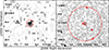 |
Fig. 1. Left panel: ACIS-S image of W0410−09 in the 0.3−7 keV energy band. The red circle shows the 2 arcsec wide region. Right panel: circular region used to extract the background. We did not consider sources detected by wavedetect and W0410−09, which are reported as crossed-out circular regions. |
We extracted the spectra using the specextract CIAO script, which creates source and background spectra and corresponding response files. We combined all the spectra and response files using the addascaspec script from the FTOOLS X-ray data and FITS files manipulation package5 to produce summed source and background spectra, and we correspondingly combined the response files.
3. Spectral analysis of W0410−09
The XSPEC (version 12.12.1) spectral fitting software was used for the spectral analysis. All the combined spectra were binned using the optimal method described by Kaastra & Bleeker (2016) and were analyzed using the Cash statistic implemented in XSPEC with direct background subtraction (W-stat; Cash 1979; Wachter et al. 1979). A Galactic column density of  was adopted (HI4PI Collaboration 2016). The spectral analysis was performed in the 0.3−7 keV energy range.
3.1. Empirical models
We started with a power-law model (POW model) that we only modified by the absorption from our interstellar galactic medium, which we parameterized with the TBABS model. This resulted in a best-fit model (C stat/d.o.f. = 46.1/48, Fig. 2) with a photon index Γ = 0.20 ± 0.25. This value is much flatter than the typical value of Γ ∼ 1.8 − 1.9 reported for QSOs (Piconcelli et al. 2005; Degli Agosti et al. 2025), and it strongly suggests that the source is highly obscured. This model indeed resulted in an X-ray bolometric correction Kbol, X = Lbol/L2 − 10 ∼ 6600, a value that appears unreasonably high compared to expectations (Duras et al. 2020). Accordingly, the POW model was modified by an intrinsic absorption term (i.e., at the redshift of W0410−09) parameterized by the ZTBABS multiplicative model. In this case, when we assumed Γ = 1.9, we obtained a very high value of NH (∼1024 cm−2). For a very high absorption column density, it is necessary to also consider the effect of Compton scattering. The absorbed model was therefore further modified with the CABS model (Arnaud 1996, XSPEC User’s Guide v12.12.1) to account for Compton scattering of X-ray photons. This model only takes the loss of photons outside of the line of sight into account. Adopting this model (CABSPOW), we obtained a best-fit parameterization (C stat/d.o.f. = 54.8/48, Fig. 2) with  . Positive residuals at the position of the Fe K-lines (6−8 keV) are clearly visible. Based on the Al Kα and Si Kα background lines, we verified at observed energies between 1.5 and 2 keV (consistent with the rest-frame energies of the positive residuals) whether they might be due to an incorrect background subtraction. To do this, we tried different background circular regions at distances up to ∼1.8 arcmin from the Hot DOG in different directions. We conclude that the residuals are not caused by a background artifact. A Gaussian line left free to vary in this energy range resulted in a best-fit energy of 7.9 ± 0.2 keV (C stat/d.o.f. = 50.5/46). This component, consistent with Fe XXV Kβ line, does not significantly improve the fit (Pnull = 0.15, according to an F test). We further investigated whether the use or addition of further lines (i.e., the Fe Kα at 6.4 keV and the Fe XXV Kα line at 6.697 keV) might improve the modeling, but the fits did not improve considerably, and the values of the parameters obtained with the model including the lines did not change significantly. For the Fe Kα line, we obtained an upper limit for the rest-frame equivalent width of 1.6 keV. A high equivalent width Fe Kα line is commonly associated with reflection in CT AGN, where the primary emission is entirely suppressed, as typically reported in CT AGN (e.g., Ghisellini et al. 1994; Matt et al. 2003; Risaliti & Elvis 2004; Hickox & Alexander 2018). Therefore, the Fe Kα upper limit is entirely consistent with the extreme CT obscuration estimated by this model. We therefore did not include the line components in the final best-fit CABSPOW model.
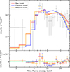 |
Fig. 2. ACIS-S Chandra spectrum of W0410−09. Empirical models are reported in different colors. The POW model is shown in red, the CABSPOW model in blue, and the REFLDOM model in orange. The spectrum was slightly rebinned for better visualization. In the lower panel, the residuals for each model are shown in the same color as their respective model. |
Because NH was so high, we also evaluated the possibility that the primary power-law spectrum is completely absorbed by matter with NH ≫ 1024 cm−2 and therefore completely dominated by the reflection component from cold material parameterized by a PEXMON model (see Fig. 2). The reflection model employs a planar geometry with an infinite optical depth, illuminated by the primary continuum. For an isotropic source, it spans an opening angle of Ω = 2π × R, where R is a parameter representing the reflection strength. We adopted this model under certain assumptions: A solar abundance, an exponential high-energy cutoff (Ec = 200 keV) applied to the primary power-law incident radiation (e.g., Fabian et al. 2015), and a reflector inclination angle of 60 deg. In this model, only the reflection component is taken into account and that of the primary is neglected, which for our purposes is considered completely absorbed (model REFLDOM). The best-fit parameterization provided an equally good but simpler fit to the data, with only the normalization free to vary (C stat/d.o.f. = 48.8/49). This suggests that the primary coronal component is obscured by a heavy CT absorber, which provides an equally good statistical representation as the previous fit of the Hot DOG spectrum. The luminosity in the 2−10 keV range of the reflected component is L2 − 10 = (1.0 ± 0.1)×1044 erg s−1. Since the NH of the absorber is unconstrained in this case, it is not possible to calculate the absorption-corrected (i.e., intrinsic) luminosity of the coronal component. The derived parameters for all the empirical models we used in our analysis are reported in Table 2.
Best-fit parameters derived from the empirical models.
3.2. Geometry-dependent obscuration models
To obtain more accurate and physically motivated constraints, we used two different models derived from Monte Carlo radiative transfer simulations employing a toroidal geometry for the obscurer and in which the X-ray source was located at the geometrical center of the absorbing structure that obscures and reprocesses the X-ray power-law-shaped emission. The first model approximated the torus geometry by employing a spherical absorber, with polar cutouts with variable half-opening angle θtor (Baloković et al. 2018, hereafter BORUS). The second model employed a doughnut torus geometry with a fixed θtor = 60 deg (Murphy & Yaqoob 2009; Yaqoob 2012, hereafter MYTORUS). Both models adopted a uniform density obscurer, in which the gas was assumed to be cold and neutral, and takes the Compton scattering into account. Fluorescent line emission and the reprocessed continuum were calculated self-consistently. The gas was assumed to be uniformly distributed, with elemental abundances similar to those of the Sun. Neutral K-shell α and β transitions at ∼6−7 keV were calculated for Fe and Ni by both models. BORUS includes Kα and Kβ transitions from elements up to zinc (Z < 31).
3.2.1. Borus model
BORUS assumes a primary spectral component in the form of a power law with a high-energy exponential cutoff and provides a table model that only includes the reprocessed spectral components (continuum and lines). It therefore needs to be used in conjunction with the primary component. We fit the ACIS spectrum adopting this model in XSPEC,
![Mathematical equation: $$ \begin{aligned} tbabs \ (ztbabs \times cabs \times zcutoffpl + Borus +[zgauss ]), \end{aligned} $$](/articles/aa/full_html/2026/01/aa56627-25/aa56627-25-eq18.gif) (1)
(1)
where TBABS is the photoelectric Galactic absorption term, ZCUTOFFPL is the primary redshifted power-law component with a high-energy exponential cutoff that was modified by the photoelectric absorption at the redshift of the source (ZTBABS), and the Compton scattering terms (CABS). The torus table model BORUS accounts for the reprocessing by the geometrical toroidal structure. In our fits, we also evaluated the need for an additional Gaussian component (ZGAUSS) to better describe the possible presence of an ionized Fe K-line at ∼7−8 keV rest frame (see Sect. 3.1).
The BORUS table model only accounts for Γ values in the range 1.4−2.6. Because of the few spectral counts, Γ would only be loosely constrained over this wide range. Therefore, we performed our fits with Γ fixed to 1.9, which is the slope typically expected for AGN and measured in QSOs at cosmic noon and in this luminosity regime (e.g., Nardini et al. 2019; Zappacosta et al. 2020). We also set θtor, inclination angle (θinc), cutoff energy (Ecut), and iron abundance (Afe) to 60 deg (equal to MYTORUS for a consistent comparison), 80 deg (i.e., almost edge-on), 200 keV, and solar, respectively. The best-fit BORUS model gives NH ∼ 0.9 × 1024 cm−2 (C stat/d.o.f. = 54.6/48, see Fig. 3 left panel). We included a ZGAUSS component to account for residuals at ∼7−8 keV rest frame. The best-fit modeling, resulting in a line energy of Egauss = 7.9 ± 0.2 keV (C stat/d.o.f. = 48.4/46), did not significant improve the fit (Pnull = 0.06 according to an F test). We also tried a model with θtor = 0 (i.e., a sphere without polar cutouts; hereafter BORSPHERE). In this case, the best-fit model did not need a ZGAUSS component and returned a value of NH ∼ 1.3 × 1024 cm−2, but with a lower fit statistics (C stat/d.o.f. = 58.3/48) and high residuals (see Fig. 3 right panel) in the entire energy range. The derived parameters for the BORUS and BORSPHERE modeling are reported in Table 3.
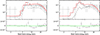 |
Fig. 3. Left panel: ACIS-S Chandra spectrum with BORUS model and residuals. The solid red line represents the best-fit model, the dotted line represents the reflection component, and the dashed line represents the highly absorbed power-law continuum with an exponential cutoff. The spectra are slightly rebinned for better visualization. Right panel: ACIS-S Chandra spectrum with the BORSPHERE model and residuals. The solid red line represents the best-fit model, the dotted line represents the Compton reflection component, and the dashed line indicates the absorbed cutoff power-law component. |
Best-fit parameters derived from geometry-dependent models.
3.2.2. MYTorus model
The MYTORUS implementation in XSPEC consists of three different table model components: (1) one component for the attenuation of the line-of-sight radiation caused by photoelectric and Compton-scattering effects (MYTZ), (2) another component to reprocess the Compton-scattered radiation (MYTS), (3) and a final component that calculates the contribution from fluorescent line emission (MYTL). Therefore, the XSPEC parameterization of this model is
![Mathematical equation: $$ \begin{aligned} tbabs \ ( zpow \times MYTZ + c_{s} \times MYTS + c_{l} \times MYTL +[zgauss ]), \end{aligned} $$](/articles/aa/full_html/2026/01/aa56627-25/aa56627-25-eq29.gif) (2)
(2)
where ZPOW is the redshifted power-law component, and cs and cl are the normalization constants of MYTS and MYTL, respectively. In our parameterization, the three components were applied progressively in sequence, adding one at a time to the previous component to determine the best model description of the data. The three components initially shared the same absorber column density and were combined with normalization constants (cs and cl) that were initially set to unity. To match the geometric requirements imposed by standard unification schemes in which Type II sources are observed at high inclinations and to account for the high column density, we set an almost edge-on view of the torus at θinc = 80 deg. We assumed Γ = 1.9 for the slope of the continuum power law. MYTORUS provides an estimate of the equatorial column density,  , which is defined as the equivalent hydrogen column density through the diameter of the tube of the torus. The actual line of sight NH, is the NH quantity measured in the empirical models, and it translates in BORUS for this particular torus aperture (θtor = 60 deg) into
  . All components were connected to the same
  .
.
We started by employing a model using the MYTZ component. We obtained a best-fit model with C stat/d.o.f. = 54.4/48 and a column density NH ∼ 0.9 × 1024 cm−2. The poor parameterization is mainly given by the highly negative residuals at energies 10−15 keV rest frame, corresponding to 2−3 keV observed energies. Therefore, we added a scattered MYTS component. This resulted in an NH ∼ 0.9 × 1024 cm−2, which was obtained with a C stat/d.o.f. = 54.2/48. We also attempted to decouple the NH values of the two components, considering that the absorbed portion along the line of sight might have a different column density than the scattered medium. This test considerably improved our fit with a C stat/d.o.f. = 46.5/47, but required a line-of-sight column density of NH ∼ 4.6 × 1024 cm−2 and a column density from the MYTS component of only 1022 cm−2, which is highly unlikely and would indicate strong obscuration exclusively along the line of sight. Hence, we recoupled the NH values and added a line component (MYTL) to account for line residuals at 6−7 keV. We obtained a best-fit column density of NH ∼ 1.0 × 1024 cm−2 (C stat/d.o.f.= 53.7/48). The model shows a positive residual at 7−8 keV. Following the previous attempts, we added an additional Gaussian component (ZGAUSS) to account for the positive residual at ∼7.9 keV and obtained a best-fit model with a C stat/d.o.f. = 47.1/46. An F test between the models with and without the ZGAUSS component returned Pnull = 0.05, indicating a marginal statistical improvement, but the rest-frame equivalent width is 3.6 keV, which is extreme for these lines in heavily obscured AGN. Therefore, we prefer to ascribe it to a statistical fluctuation and retained as the best-fit fiducial model the model without the Gaussian component.
The derived best-fit column density is NH ∼ 1.4 × 1024 cm−2. It is not strongly constrained, however, and by enlarging the search for a best-fit NH to the entire parameter space including the NH = 1025 cm−2 hard limit for the MYTORUS model, we obtained a better best fit (C stat/d.o.f. = 48.6/48) with NH pegged to 1025 cm−2. In this case, we were only able tomeasure a lower limit of 6.9 × 1024 cm−2. Given the very high NH, we estimated as 1.2 ± 0.9 keV the equivalent width relative to the Fe Kα line by substituting the MYTL component with an unresolved Gaussian line at a fixed energy of 6.4 keV and left the other MYTORUS components at their best-fit values. Table 3 reports the derived parameters for this model.
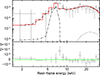 |
Fig. 4. ACIS-S Chandra spectrum with the MYTORUS model and residuals. The solid red line represents the best-fit model, the dashed line indicates the absorbed component, the dotted line represents the Compton-scattered component, and the dot-dashed line denotes the lines component. The spectrum was slightly rebinned for better visualization. |
4. X-ray emission from the companion overdensity
Ginolfi et al. (2022) reported the discovery of a significant overdensity of Lyα emitters (LAEs) surrounding the hyperluminous QSO W0410−09, suggesting a highly star-forming and dense environment. The LAEs are spectroscopically confirmed through the detection of the Lyα emission line, which provides reliable redshift measurements. The median redshift of the sources is consistent with that of the Hot DOG, suggesting that W0410−09 dominates the environment and lies at the center of the gravitational potential well of the halo. The Lyα luminosities lie in the range ![Mathematical equation: $ \log\, (L_{\mathrm{Ly}\alpha}\,[\mathrm{erg\,s}^{-1}]) \sim 41.8{-}42.65 $](/articles/aa/full_html/2026/01/aa56627-25/aa56627-25-eq33.gif) , and the star formation rates (SFRs) are ∼12−100 M⊙ yr−1.
, and the star formation rates (SFRs) are ∼12−100 M⊙ yr−1.
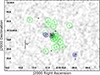 |
Fig. 5. ACIS-S image in the 0.3−7 keV energy band showing the 24 LAEs. The 19 companions associated with the Hot DOG are highlighted with green crosses, while those unrelated are indicated with black squares. The green circles mark the regions we used for the companion photometry. The X-ray sources detected using the wavdetect algorithm are shown in blue. The dashed circles indicate the regions that were excluded from the companion photometry, and the Hot DOG is shown in red. |
To search for possible X-ray counterparts of the detected LAEs, we first examined the output of the detection algorithm in the broad, soft, and hard bands (see Sect. 2). Excluding the Hot DOG, we report the detection of two nearby X-ray sources in the broad and hard bands at a distance from the W0410−09 of ≳7 arcsec. They are ≳2.5 arcsec away from their nearest Lyα emitter (Fig. 5). Given the Chandra absolute pointing position accuracy and the arcsec-level point spread function, it is highly unlikely that these sources are the high-energy counterparts to the LAEs. The nondetection in the X-ray of the LAEs implies that if AGN are present in some of them, their X-ray fluxes are expected to be fainter than the detection limit of our observations. They can either be low-luminosity unobscured AGN or higher-luminosity obscured AGN. To search for these undetected AGN, we performed photometry in the broad, soft, and hard bands at the position of the LAEs. To do this, we only considered the 19 emitters associated with the Hot DOG with velocities along the line of sight in the range [−2000, +2000] km s−1 relative to the Hot DOG rest frame (they are reported in Fig. 5 as thick crosses).
For the photometry, we adopted circular regions with a radius of 3 arcsec centered on the position of the associated LAEs. We excluded the W0410−09 contribution in the central crowded region by removing the events within a radius of 3 arcsec. We constructed a single combined region that encompassed the entire sky area occupied by all the LAEs and accounted for overlapping areas, which were included only once. We did not detect significant emission in any of the three bands. We further performed photometry in the narrow rest-frame energy band 6−7 keV (observed 1.3−1.5 keV) in order to search for possible Fe Kα emission from obscured AGN hosted by the LAEs. A high equivalent width line at 6.4 keV is typically considered the hallmark of heavily obscured sources (see Sect. 3.1). We found an excess of counts that was ∼3σ significant over the background emission and corresponds to  net counts. For this reason, we ran the detection algorithm in the 6−7 keV band, and we only found emission from the Hot DOG. This evidence strongly indicates that undetected obscured AGN emission is hosted in several of the LAEs.
To estimate an upper luminosity limit for these AGN, we adopted the hard band upper limit (the most constraining of the considered bands) that was 24.6 net counts and corresponds to a count rate of 8.9 × 10⁻⁵ cts s−1. Assuming a BORUS model with NH = 5 × 1023 cm−2 (1024 cm−2) and normalizing it to this count rate, we obtained an upper limit for the 2−10 keV unabsorbed luminosity of 1046 erg s−1 (1.9 × 1046 erg s−1) that corresponds to a luminosity ≲7 × 1044 erg s−1 (1045 erg s−1) when we assume that all the LAEs host an AGN.
We finally estimated the possible thermal diffuse emission permeating the overdense protocluster region. We performed photometry in the three bands from a circular region with a radius of ∼30 arcsec centered on the Hot DOG. During this procedure, we excluded circular regions in a radius of 3 arcsec around the companions and the X-ray detected sources. We found no significant emission in excess over the background. Given the low Chandra sensitivity at low energy, we further restricted the full and soft bands to energies > 0.5 keV (i.e., we removed the 0.3−0.5 keV range, which might contribute with background-only emission). No significant diffuse emission was found in this case either. Therefore, we conclude that there is no detectable diffuse emission in the overdense region around W0410−09. Either there is no emission, or it is too weak or its temperature is too low (≪1 keV) to be detectable by Chandra.
5. Discussion
5.1. High obscuration and bolometric correction
Our analysis confirms that W0410−09 is a luminous and heavily obscured QSO shining at z ∼ 3.6. An empirical absorbed power-law parameterization accounting for Compton scattering suggests high obscuration compatible with CT levels. A similarly good description of its spectrum is a reflection-dominated model that further suggests that the source is obscured at the CT levels. Physically motivated models implementing toroidal or spherical geometry for the obscurer, properly accounting for Compton-scattering geometrical effects, still indicate a column density of ≳1024 cm−2. Depending on the adopted models, we obtain absorptions from nearly CT (∼1024 cm−2, BORUS model) to highly CT (≫1024 cm−2, MYTORUS model) levels. This large difference in the derived NH values is likely due to the different geometrical assumptions about the obscuring material in the two models. These values were obtained for toroidal obscurers with similar geometry and configuration relative to the observer, that is, θtor = 60 deg and θinc = 80 deg, respectively. The BORUS model allowed us to change θtor, and we therefore allowed it to vary in order to explore the parameter space. We obtained a best-fit model (C stat/d.o.f. = 46.6/47) with  , NH > 2.5 × 1024 cm−2, and LX > 5.4 × 1045 erg s−1. In this case, despite the tight constraints of θtor, we therefore have a loose constraint on
  that still indicates a CT obscurer.
Its extremely high bolometric luminosity of 6.4 × 1047 erg s−1 (Díaz-Santos et al. 2021) places W0410−09 among the most luminous and obscured z > 3 AGN ever reported so far, as shown by the NH versus Lbol plot of highly luminous AGN (Lbol > 1047 erg s−1, see Fig. 6). The bolometric luminosity of the target was conservatively calculated by Tsai et al. (2015) by integrating the photometric data with a power law interpolated between observed flux density measurements.
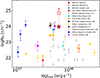 |
Fig. 6. Spectroscopically derived NH vs. Lbol for a sample of luminous and X-ray obscured QSOs with |
We estimated a L2 − 10 range from ∼(1.3 − 1.4)×1045 erg s−1 (BORUS) to > 1046 erg s−1 (MYTORUS). From these values, we calculated Kbol, X = Lbol/L2 − 10, which is defined as the conversion factor used to estimate the bolometric luminosity from the X-ray luminosity. We obtained the following X-ray bolometric corrections:  and
and  . Fig. 7 illustrates the recent Kbol versus Lbol relation for Type II AGN derived by Duras et al. (2020). They reported Kbol, X of W0410−09 for the two toroidal models. From the relation calibrated by Duras et al. (2020), we obtained for W0410−09 a Kbol, X ∼ 390, which is consistent with the parameters estimated with the BORUS models. The MYTORUS modeling would imply an extremely high L2 − 10 and a very low Kbol value (see Fig. 7), which were rarely reported for hyperluminous QSOs at cosmic noon so far (e.g., Stern 2015; Martocchia et al. 2017; Lansbury et al. 2020; Zappacosta et al. 2020). In addition, the L2 − 10 keV versus L6 μm plot reported in Fig. 8 shows that the L2 − 10 derived by BORUS parameterization agrees with the location of other hyperluminous Hot DOGs and QSOs and with the best-fit relations reported in the literature. The location for the MYTORUS modeling is at least more than one order of magnitude, which disagrees with the data and the empirical relations. In order to bring this in agreement, we would need to have higher L6 μm by an order of magnitude at least.
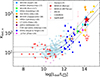 |
Fig. 7. Hard X-ray bolometric correction band as a function of the Lbol for Type II AGN. The filled and empty red stars indicate the BORUS and MYTORUS parameterizations, respectively, compared to other samples. In particular, we only include the WISSH QSOs with NH > 1023 cm−2 (gray circles; Martocchia et al. 2017). The light black lines show the best fit (continuous line) and dispersion (dashed lines) of the Kbol, X − Lbol relation for Type II QSOs from Duras et al. (2020). We also plot the ASCA, COSMOS, and Swift-BAT samples, which only include Type II AGN. |
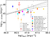 |
Fig. 8. L2 − 10 keV vs. L6 μm relation for QSOs with Lbol > 1047 erg s−1. The filled and empty red stars represent W0410−09 for the BORUS and MYTORUS models, respectively. The Hot DOGs are represented with stars of different colors, as in Fig. 6. The gray points and red dots represent the X-WISSH hyperluminous Type I QSO sample (Martocchia et al. 2017) and two reddened QSOs (Martocchia et al. 2017). We also report X-ray-to-MIR relations derived for different optical, MIR, and X-ray selected AGN samples (Fiore et al. 2009; Lanzuisi et al. 2009; Stern 2015; Chen et al. 2017). |
5.2. The blow-out phase and the circumgalactic nebula
Hot DOGs are Type II QSOs and are therefore not expected to show broad lines from virialized nuclear regions. In principle, SMBH masses and the inferred Eddington ratios (indicative of their accretion rates) can therefore not be estimated with broad emission lines via single-epoch virial mass estimators. Despite this, broad lines have been reported in several Hot DOGs. They are often measured to have high blueshifts that are indicative of unvirialized motions perhaps caused by nuclear outflows (e.g., Finnerty et al. 2020; Jun et al. 2020; Ginolfi et al. 2022), which likely lead to biased mass estimates on these sources. Nonetheless masses of about 109−1010 M⊙ have been measured via the Balmer, Mg II, or C IV emission lines (Wu et al. 2018; Tsai et al. 2018; Li et al. 2024). In particular, Li et al. (2024) measured the SMBH masses for a peculiar type of Hot DOGs showing blue excess emission in the UV-optical band, which exceeds the starburst component from the host galaxy. This is consistent with the spectral energy distribution of Type I sources, which might be caused by AGN emission that is scattered outside the obscuring nuclear material (Assef et al. 2016, 2020). Li et al. (2024) obtained masses in the range 108.7 − 1010 M⊙. These estimates were based on the C IV emission line, which might be affected by nonvirial outflowing components, and therefore, the corresponding SMBH masses might be overestimated (Baskin & Laor 2005; Sulentic et al. 2007; Denney 2012; Coatman et al. 2017; Vietri et al. 2018).
The same calculation for the more traditional Hot DOGs gave estimates in roughly the same mass range, which indicates that if Hot DOGs and their blue excess variant are the same sources, we can roughly trust the estimated masses on the reported broad lines for standard Hot DOGs. In this case, the reported mass range is consistent with the mass range measured for hyperluminous Type I QSOs (e.g., Vietri et al. 2018; Trefoloni et al. 2023) at cosmic noon. This provides a first-order indication that Hot DOGs accrete close to the Eddington rate, with Eddington ratios of λEdd ∼ 0.1 − 4 (Li et al. 2024).
Figure 9 reports the location of the Hot DOGs in the NH versus λEdd plane. Hot DOGs are located in the upper level of the so-called blow-out region. A source populating this region is subject to winds originating from strong radiative pressure on the nuclear dusty gas (Fabian et al. 2006, 2008), which eventually clears out the surrounding region. This is predicted within the framework of the radiation-regulated unification model (e.g., Jun et al. 2021; Toba et al. 2022; Ricci et al. 2023). In this model, AGN dynamically evolve through the NH versus λEdd plane during their life cycle, transitioning from obscured to unobscured phases under the influence of winds. The highly blueshifted broad UV lines, as reported by Ginolfi et al. (2022), further corroborate the Hot DOG’s blow-out phase. We report W0410−09 at λEdd = 1 and indicate the λEdd range corresponding to the SMBH mass range reported by Li et al. (2024). Similarly to other Hot DOGs, the source is located entirely in the blow-out region. It is important to note that most SMBH mass estimates used to calculate λEdd relied on the FWHM of the CIV emission line, which might be affected by outflows (i.e., overestimated SMBH masses, and therefore, lower λEdd). As a result, the true λEdd values might be higher, and the sources would shift further to the right in the NH versus λEdd plane. Along with the Hot DOGs, we also report hyperluminous high-redshift reddened QSOs and local low-luminosity AGN for comparison. The fact that we observe a nebula significantly smaller than the average size of nebulae reported for Type I QSOs (e.g., Borisova et al. 2016; Arrigoni Battaia et al. 2019; Cai et al. 2019; Fossati et al. 2021) and that the nuclear emission is obscured by a star formation medium suggests that the ionizing flux (both X-ray and, especially, UV) is likely blocked and unable to produce an extended nebula, as it arrives strongly attenuated or extinguished on CG scales. This scenario is supported by observational and theoretical evidence regarding CGLANs around these systems. González Lobos et al. (2023) demonstrated that dustier systems have smaller CGLANs than Type I QSOs. These observational findings agree with theoretical predictions by Costa et al. (2022), who showed that nebula emission from obscured sources (in their case, edge-on views) appears to be weak and therefore smaller than expected for a face-on source with similar AGN luminosity. At a fixed bolometric luminosity, the system seen edge-on or face-on therefore gives a faint or bright nebula, respectively.
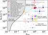 |
Fig. 9. NH vs. λEdd. We only compare sources with NH derived from spectral analysis. We report as colored points the luminous QSOs and in gray Swift-BAT low-luminosity AGN (Ricci et al. 2017b). The filled and empty red stars represent W0410−09 for the BORUS and MYTORUS models, respectively. The hatched light blue region represents the range of NH values derived from previous Hot DOG X-ray analyses (Assef et al. 2016; Vito et al. 2018; Zappacosta et al. 2018), and the λEdd range was determined using the BH masses estimated by Li et al. (2024, see our Sect. 5.2 for details). For hyperluminous optical QSOs, we show ±1σ range of λEdd values for the most luminous QSOs at z ≳ 2 in SDSS DR3 (downward-pointing light blue triangle marker, plotted at NH = 1021 cm−2). The crosses show local (z ∼ 0.037) Swift-BAT AGN (Ricci et al. 2017b). The light gray zone represents the blow-out region for radiation trapping, where the radiation emitted by the black hole is trapped in the surrounding gas through a process of repeated absorption and reemission, causing continuous heating and accelerating the gas outward (Ishibashi et al. 2018). The white zone indicates the blow-out region in the single-scattering approximation. Below, the dot-dashed line separates nuclear from the host-scale absorption. |
Consistent with this scenario, W0410−09 exhibits a CGLAN with a spatial extent of approximately 30 kpc (Ginolfi et al. 2022), which is smaller by about a factor of three than the typical sizes observed around unobscured quasars, which generally reach ∼100 kpc (Borisova et al. 2016; Arrigoni Battaia et al. 2019; Travascio et al. 2020 and references therein). Ideally, for an obscuration with a geometry close to 4π, as expected from the chaotic accretion scenario predicted by the merger-driven QSO formation model, the fact that we observe a nebula suggests that some leaked UV emission powers the nebula, which implies that the covering factor of the obscuring CT medium might be < 1.
5.3. Environment
The identification of Lyα emitting companions in the UV rest-frame analysis of the VLT−MUSE field of W0410−09 by Ginolfi et al. (2022) prompted us to perform a more detailed investigation of their nuclear properties taking advantage of the exquisite Chandra spatial resolution in our deep observation. Within the W0410−09 environment, our analysis did not detect significant X-ray emission coincident with the 19 LAE companions. W0410−09 represents the sole LAE in the field exhibiting X-ray emission. Based on the Hot DOG alone, we therefore estimated an AGN fraction  , where uncertainties were calculated assuming small number statistics (Gehrels 1986). The detection of significant emission from the LAE only in the spectral region corresponding to the Fe Kα line and not in the broad energy bands strongly suggests, however, that heavily obscured (CT) AGN are hosted in many of the LAEs. We performed a crude estimation of the possible number of LAEs hosting an obscured AGN by lowering the detection threshold to the 90% level (i.e., selecting LAEs with ≥2 X-ray counts in the 6−7 keV rest-frame). Under this assumption, we identified six sources as detected. Adding these unresolved sources to the AGN fraction calculation, we found roughly
  . Fig. 10 (left panel) reports the AGN fraction (fAGN*), measured for distinct galaxy populations selected adopting different tracers, as a function of redshift for high-z protocluster overdensities. Our
  estimate is consistent within the uncertainties with the
  values reported in the literature and ranges from 2% to 19% (Lehmer et al. 2009; Digby-North et al. 2010; Tozzi et al. 2022; Vito et al. 2024). In any case, we expect fAGN* to be function of the limiting X-ray flux of the surveyed field. Therefore, we calculated the X-ray luminosity limit (LX, lim) reached by our observation of the W0410−09 overdensity. We estimated a 0.5−7 keV count-rate limit of 6.3 × 10⁻⁵ (90% confidence level). By assuming a power law with Γ = 1.9 absorbed by a Galactic NH = 4.03 × 1020 cm−2, we estimated a 0.5−7 keV flux of 8.9 × 10⁻¹⁶ erg cm−2 s−1, which at the redshift of the Hot DOG corresponds to an unabsorbed (i.e., intrinsic) 2−10 keV luminosity limit of < 5.5 × 1043 erg s−1. Fig. 10 (right panel) shows
  as a function of LX, lim for the protocluster overdense regions targeted in X-rays. We found no clear trend between
  and LX, lim and cannot confirm that AGN activity in LAEs is low in field and protoclusters, as reported in previous works (e.g., Malhotra et al. 2003; Zheng et al. 2016). Similar fractions and a lack of trends are also reported for the fAGN* measured in other galaxy populations selected by different tracers (see Fig. 10). For a proper comparison among the AGN fractions, the surveyed area volume needs to be taken into account. Furthermore, there are indications that
  depend on the luminosities of the LAEs (Nilsson & Møller 2011). In this comparison, these corrections were not applied or tested. Further investigations of AGN fraction in our field with different tracers that also include Hα emitters, Lyman-break galaxies, and submillimeter galaxies, as reported by Vito et al. (2024), for instance, are needed to estimate the AGN fraction in the Hot DOG environment better. This will help us to understand the relevance of different mechanisms, such as galaxy interactions (Ehlert et al. 2015), ram pressure (Poggianti et al. 2017), and cold gas accretion (Gaspari et al. 2015), which likely cause AGN activity at different scales in these dense environments.
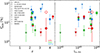 |
Fig. 10. Left panel: fraction of X-ray-selected AGN among galaxies with different selection criteria in dense environment for high-z overdensities, as reported in the literature (Lehmer et al. 2009; Digby-North et al. 2010; Lehmer et al. 2013; Krishnan et al. 2017; Macuga et al. 2019; Vito et al. 2020; Polletta et al. 2021; Tozzi et al. 2022; Vito et al. 2024; Travascio et al. 2025). Right panel: X-ray luminosity limit vs. AGN fraction in dense environments for high-redshift overdensities. Our measurements are shown as red diamonds. A filled diamond represents the fraction of AGN directly detected among the LAEs, and an empty diamond refers to the unresolved AGN fraction inferred from the stacking analysis at the 90% confidence level. The colors of the points in the graph indicate the different selection criteria: red for LAEs, green for Hα-emitting galaxies (HEAs), and blue for submillimeter-selected dusty star-forming galaxies (DSFGs). The fAGN* of MQN01 is calculated including M* > 1010.5 M⊙ galaxies (Travascio et al. 2025). |
6. Conclusion
We presented the X-ray analysis of ∼280 ks Chandra observation targeting W0410−09 and its environment. The Hot DOG is significantly detected with ∼74 net counts in the full band (0.3−7 keV), which makes W0410−09 the most significantly detected Hot DOG in the X-rays. We extracted its spectrum and performed an extensive X-ray spectral modeling. The X-ray spectrum is flat and dominated by a clear emission feature at ∼7 keV rest frame. These are signatures of heavily obscured X-ray emission. For this analysis, we used phenomenological and physically motivated models for the nuclear obscuration. The latter accounts for the geometry of the obscurer and for an accurate treatment of the X-ray reprocessing due to Compton reflection. We explored two scenarios: 1) an edge-on torus, and 2) a sphere isotropically covering the nucleus. We list our main conclusions below.
-
In all cases, a significant degree of obscuration was measured. The column densities range from nearly CT (
![Mathematical equation: $ \log [N_{\mathrm{H}}/\mathrm{cm}^{-2}] \sim 24 $](/articles/aa/full_html/2026/01/aa56627-25/aa56627-25-eq47.gif) ) to heavy CT (
) to heavy CT (![Mathematical equation: $ \log [N_{\mathrm{H}}/\rm cm^{-2}] \gg 24 $](/articles/aa/full_html/2026/01/aa56627-25/aa56627-25-eq48.gif) ) levels. This makes W0410−09 one of the most obscured (if not the most obscured) and luminous z > 3.5 AGN X-ray detected so far.
) levels. This makes W0410−09 one of the most obscured (if not the most obscured) and luminous z > 3.5 AGN X-ray detected so far. -
We measured the intrinsic luminosity in the hard band (between 2 and 10 keV) for W0410−09, finding it to be
 . This agrees with standard relations reported for Kbol, x versus Lbol and L2 − 10 keV versus L6 μm;
 -
At the likely high Eddington ratio reported for Hot DOGs by previous works, this level of obscuration suggests that W0410−09 is undergoing a blow-out phase in which the strong pressure of the UV disk emission on the dusty nuclear obscurer is able to overcome the SMBH gravitational pull by blowing the circumnuclear dusty gas out as a wind.
Unlike hyperluminous unobscured QSOs at cosmic noon, which exhibit giant (100 kpc) CGLANs around them, our highly obscured QSO only shows a small 30 kpc nebula, suggesting that the stronger nuclear obscuration primarily blocks the radiative and mechanical energy transport to CG scales. This extreme obscuration agrees with the merger-driven QSO formation scenario, in which our Hot DOG is in the blow-out phase. This is a crucial stage in the transition from an obscured to an unobscured QSO. This leads to a scenario in which 4π-distributed inhomogeneous (i.e., covering factor < 1) heavy absorption of nuclear ionizing radiation limits the powering of the Lyα nebular emission to a few tens of kpc.
Additionally, we analyzed the X-ray emission from the surrounding environment. A previous study by Ginolfi et al. (2022) revealed that W0410−09 is surrounded by a dense concentration of 19 Lyα emitting companion galaxies located within a CG region of ∼300 kpc. This characterizes the Hot DOG neighborhood as one of the densest protocluster environments reported so far. We did not detect any obvious X-ray emitting counterpart of the 19 LAEs associated with the Hot DOG. Hence, we performed photometry to measure the emission from all the emitters. No emission was detected in the broad, soft, and hard band. We report significant (3σ) emission around 6–7 keV (rest frame), however, which is likely caused by a prominent Fe Kα line emission. This indicates strongly obscured AGN hosted by several LAE. We estimated the AGN fraction from all LAEs to be  in the overdensity. This value can reach ∼35% when unresolved obscured AGN hosted by several LAEs are accounted for. This agrees with previous estimates for LAEs in other protoclusters at similar redshifts.
Our results highlight the importance of deep X-ray observations of distant heavily obscured QSOs for improving our understanding of the complex phenomenon of the assembly and evolution of the most massive galaxies. This study can be considered a pathfinder for future investigations of the nuclear properties of high-z dust-enshrouded QSOs, which constitute one of the main objectives of the new X-ray telescopes currently in the design phase.
Acknowledgments
The authors acknowledge financial support from the Bando Ricerca Fondamentale INAF 2022 Large Grant “Toward an holistic view of the Titans: multi-band observations of z > 6 QSOs powered by greedy supermassive black holes”. LZ acknowledge support from the European Union – Next Generation EU, PRIN/MUR 2022 2022TKPB2P – BIG-z. FR acknowledges financial support from the Italian Ministry for University and Research, through the grant PNRR-M4C2-I1.1-PRIN 2022-PE9-SEAWIND: Super-Eddington Accretion: Wind, INflow and Disk-F53D23001250006-NextGenerationEU. SC gratefully acknowledges support from the European Research Council (ERC) under the European Union’s Horizon 2020 Research and Innovation programme grant agreement No 864361. FV acknowledges support from the “INAF Ricerca Fondamentale 2023 – Large GO” grant. We thank Andrea Travascio for providing the MQN01 values included in Fig. 10.
References
- Arnaud, K. A. 1996, in Astronomical Data Analysis Software and Systems V, eds. G. H. Jacoby, & J. Barnes, ASP Conf. Ser., 101, 17 [NASA ADS] [Google Scholar]
- Arrigoni Battaia, F., Hennawi, J. F., Prochaska, J. X., et al. 2019, MNRAS, 482, 3162 [NASA ADS] [CrossRef] [Google Scholar]
- Arrigoni Battaia, F., Prochaska, J. X., Hennawi, J. F., et al. 2018, MNRAS, 473, 3907 [NASA ADS] [CrossRef] [Google Scholar]
- Assef, R. J., Walton, D. J., Brightman, M., et al. 2016, ApJ, 819, 111 [Google Scholar]
- Assef, R. J., Brightman, M., Walton, D. J., et al. 2020, ApJ, 897, 112 [NASA ADS] [CrossRef] [Google Scholar]
- Baloković, M., Brightman, M., Harrison, F. A., et al. 2018, ApJ, 854, 42 [Google Scholar]
- Baskin, A., & Laor, A. 2005, MNRAS, 356, 1029 [NASA ADS] [CrossRef] [Google Scholar]
- Borisova, E., Cantalupo, S., Lilly, S. J., et al. 2016, ApJ, 831, 39 [Google Scholar]
- Bridge, C. R., Blain, A., Borys, C. J. K., et al. 2013, ApJ, 769, 91 [Google Scholar]
- Cai, Z., Cantalupo, S., Prochaska, J. X., et al. 2019, ApJS, 245, 23 [Google Scholar]
- Cantalupo, S., Arrigoni-Battaia, F., Prochaska, J. X., Hennawi, J. F., & Madau, P. 2014, Nature, 506, 63 [Google Scholar]
- Cash, W. 1979, ApJ, 228, 939 [Google Scholar]
- Chen, C.-T. J., Hickox, R. C., Goulding, A. D., et al. 2017, ApJ, 837, 145 [Google Scholar]
- Coatman, L., Hewett, P. C., Banerji, M., et al. 2017, MNRAS, 465, 2120 [Google Scholar]
- Costa, T., Arrigoni Battaia, F., Farina, E. P., et al. 2022, MNRAS, 517, 1767 [NASA ADS] [CrossRef] [Google Scholar]
- Degli Agosti, C., Vignali, C., Piconcelli, E., et al. 2025, A&A, 702, A114 [NASA ADS] [CrossRef] [EDP Sciences] [Google Scholar]
- Denney, K. D. 2012, ApJ, 759, 44 [NASA ADS] [CrossRef] [Google Scholar]
- Dey, A., Soifer, B. T., Desai, V., et al. 2008, ApJ, 677, 943 [NASA ADS] [CrossRef] [Google Scholar]
- Díaz-Santos, T., Assef, R. J., Blain, A. W., et al. 2018, Science, 362, 1034 [Google Scholar]
- Díaz-Santos, T., Assef, R. J., Eisenhardt, P. R. M., et al. 2021, A&A, 654, A37 [NASA ADS] [CrossRef] [EDP Sciences] [Google Scholar]
- Digby-North, J. A., Nandra, K., Laird, E. S., et al. 2010, MNRAS, 407, 846 [NASA ADS] [CrossRef] [Google Scholar]
- Duras, F., Bongiorno, A., Ricci, F., et al. 2020, A&A, 636, A73 [NASA ADS] [CrossRef] [EDP Sciences] [Google Scholar]
- Ehlert, S., Allen, S. W., Brandt, W. N., et al. 2015, MNRAS, 446, 2709 [Google Scholar]
- Eisenhardt, P. R. M., Wu, J., Tsai, C.-W., et al. 2012, ApJ, 755, 173 [Google Scholar]
- Fabian, A. C., Celotti, A., & Erlund, M. C. 2006, MNRAS, 373, L16 [NASA ADS] [Google Scholar]
- Fabian, A. C., Vasudevan, R. V., & Gandhi, P. 2008, MNRAS, 385, L43 [NASA ADS] [CrossRef] [Google Scholar]
- Fabian, A. C., Lohfink, A., Kara, E., et al. 2015, MNRAS, 451, 4375 [Google Scholar]
- Fan, L., Han, Y., Fang, G., et al. 2016a, ApJ, 822, L32 [Google Scholar]
- Fan, L., Han, Y., Nikutta, R., Drouart, G., & Knudsen, K. K. 2016b, ApJ, 823, 107 [Google Scholar]
- Fan, L., Knudsen, K. K., Fogasy, J., & Drouart, G. 2018, ApJ, 856, L5 [Google Scholar]
- Finnerty, L., Larson, K., Soifer, B. T., et al. 2020, ApJ, 905, 16 [Google Scholar]
- Fiore, F., Puccetti, S., Brusa, M., et al. 2009, ApJ, 693, 447 [NASA ADS] [CrossRef] [Google Scholar]
- Fossati, M., Fumagalli, M., Lofthouse, E. K., et al. 2021, MNRAS, 503, 3044 [NASA ADS] [CrossRef] [Google Scholar]
- Frey, S., Paragi, Z., Gabányi, K. É., & An, T. 2016, MNRAS, 455, 2058 [Google Scholar]
- Gaspari, M., Brighenti, F., & Temi, P. 2015, A&A, 579, A62 [NASA ADS] [CrossRef] [EDP Sciences] [Google Scholar]
- Gehrels, N. 1986, ApJ, 303, 336 [Google Scholar]
- Ghisellini, G., Haardt, F., & Matt, G. 1994, MNRAS, 267, 743 [Google Scholar]
- Ginolfi, M., Piconcelli, E., Zappacosta, L., et al. 2022, Nat. Commun., 13, 4574 [NASA ADS] [CrossRef] [Google Scholar]
- González Lobos, V., Arrigoni Battaia, F., Chang, S.-J., et al. 2023, A&A, 679, A41 [NASA ADS] [CrossRef] [EDP Sciences] [Google Scholar]
- Hennawi, J. F., Prochaska, J. X., Cantalupo, S., & Arrigoni-Battaia, F. 2015, Science, 348, 779 [Google Scholar]
- HI4PI Collaboration (Ben Bekhti, N., et al.) 2016, A&A, 594, A116 [NASA ADS] [CrossRef] [EDP Sciences] [Google Scholar]
- Hickox, R. C., & Alexander, D. M. 2018, ARA&A, 56, 625 [Google Scholar]
- Hopkins, P. F., Hernquist, L., Cox, T. J., et al. 2006, ApJS, 163, 1 [Google Scholar]
- Ishibashi, W., Fabian, A. C., & Maiolino, R. 2018, MNRAS, 476, 512 [NASA ADS] [Google Scholar]
- Jones, S. F., Blain, A. W., Stern, D., et al. 2014, MNRAS, 443, 146 [Google Scholar]
- Jun, H. D., Assef, R. J., Bauer, F. E., et al. 2020, ApJ, 888, 110 [Google Scholar]
- Jun, H. D., Assef, R. J., Carroll, C. M., et al. 2021, ApJ, 906, 21 [Google Scholar]
- Kaastra, J. S., & Bleeker, J. A. M. 2016, A&A, 587, A151 [NASA ADS] [CrossRef] [EDP Sciences] [Google Scholar]
- Krishnan, C., Hatch, N. A., Almaini, O., et al. 2017, MNRAS, 470, 2170 [NASA ADS] [CrossRef] [Google Scholar]
- Lansbury, G. B., Banerji, M., Fabian, A. C., & Temple, M. J. 2020, MNRAS, 495, 2652 [Google Scholar]
- Lanzuisi, G., Piconcelli, E., Fiore, F., et al. 2009, A&A, 498, 67 [NASA ADS] [CrossRef] [EDP Sciences] [Google Scholar]
- Lehmer, B. D., Alexander, D. M., Geach, J. E., et al. 2009, ApJ, 691, 687 [Google Scholar]
- Lehmer, B. D., Lucy, A. B., Alexander, D. M., et al. 2013, ApJ, 765, 87 [NASA ADS] [CrossRef] [Google Scholar]
- Li, G., Assef, R. J., Tsai, C.-W., et al. 2024, ApJ, 971, 40 [NASA ADS] [CrossRef] [Google Scholar]
- Macuga, M., Martini, P., Miller, E. D., et al. 2019, ApJ, 874, 54 [NASA ADS] [CrossRef] [Google Scholar]
- Magnelli, B., Lutz, D., Santini, P., et al. 2012, A&A, 539, A155 [NASA ADS] [CrossRef] [EDP Sciences] [Google Scholar]
- Malhotra, S., Wang, J. X., Rhoads, J. E., Heckman, T. M., & Norman, C. A. 2003, ApJ, 585, L25 [NASA ADS] [CrossRef] [Google Scholar]
- Martin, D. C., Chang, D., Matuszewski, M., et al. 2014, ApJ, 786, 106 [NASA ADS] [CrossRef] [Google Scholar]
- Martocchia, S., Piconcelli, E., Zappacosta, L., et al. 2017, A&A, 608, A51 [NASA ADS] [CrossRef] [EDP Sciences] [Google Scholar]
- Matt, G., Fabian, A. C., Guainazzi, M., et al. 2003, MNRAS, 342, 422 [NASA ADS] [CrossRef] [Google Scholar]
- Murphy, K. D., & Yaqoob, T. 2009, MNRAS, 397, 1549 [Google Scholar]
- Nardini, E., Lusso, E., Risaliti, G., et al. 2019, A&A, 632, A109 [NASA ADS] [CrossRef] [EDP Sciences] [Google Scholar]
- Nilsson, K. K., & Møller, P. 2011, A&A, 527, L7 [NASA ADS] [CrossRef] [EDP Sciences] [Google Scholar]
- Piconcelli, E., Jimenez-Bailón, E., Guainazzi, M., et al. 2005, A&A, 432, 15 [NASA ADS] [CrossRef] [EDP Sciences] [Google Scholar]
- Piconcelli, E., Vignali, C., Bianchi, S., et al. 2015, A&A, 574, L9 [NASA ADS] [CrossRef] [EDP Sciences] [Google Scholar]
- Poggianti, B. M., Jaffé, Y. L., Moretti, A., et al. 2017, Nature, 548, 304 [Google Scholar]
- Polletta, M., Soucail, G., Dole, H., et al. 2021, A&A, 654, A121 [NASA ADS] [CrossRef] [EDP Sciences] [Google Scholar]
- Ricci, C., Bauer, F. E., Treister, E., et al. 2017a, MNRAS, 468, 1273 [NASA ADS] [Google Scholar]
- Ricci, C., Trakhtenbrot, B., Koss, M. J., et al. 2017b, ApJS, 233, 17 [Google Scholar]
- Ricci, C., Ichikawa, K., Stalevski, M., et al. 2023, ApJ, 959, 27 [NASA ADS] [CrossRef] [Google Scholar]
- Risaliti, G., & Elvis, M. 2004, in Supermassive Black Holes in the Distant Universe, ed. A. J. Barger, Astrophysics and Space Science Library, 308, 187 [Google Scholar]
- Sanders, D. B., Soifer, B. T., Elias, J. H., et al. 1988, ApJ, 325, 74 [Google Scholar]
- Stanley, F., Knudsen, K. K., Aalto, S., et al. 2021, A&A, 646, A178 [NASA ADS] [CrossRef] [EDP Sciences] [Google Scholar]
- Stern, D. 2015, ApJ, 807, 129 [Google Scholar]
- Sulentic, J. W., Bachev, R., Marziani, P., Negrete, C. A., & Dultzin, D. 2007, ApJ, 666, 757 [NASA ADS] [CrossRef] [Google Scholar]
- Toba, Y., Liu, T., Urrutia, T., et al. 2022, A&A, 661, A15 [NASA ADS] [CrossRef] [EDP Sciences] [Google Scholar]
- Tozzi, P., Pentericci, L., Gilli, R., et al. 2022, A&A, 662, A54 [NASA ADS] [CrossRef] [EDP Sciences] [Google Scholar]
- Travascio, A., Zappacosta, L., Cantalupo, S., et al. 2020, A&A, 635, A157 [NASA ADS] [CrossRef] [EDP Sciences] [Google Scholar]
- Travascio, A., Cantalupo, S., Tozzi, P., et al. 2025, A&A, 694, A165 [NASA ADS] [CrossRef] [EDP Sciences] [Google Scholar]
- Trefoloni, B., Lusso, E., Nardini, E., et al. 2023, A&A, 677, A111 [NASA ADS] [CrossRef] [EDP Sciences] [Google Scholar]
- Tsai, C.-W., Eisenhardt, P. R. M., Wu, J., et al. 2015, ApJ, 805, 90 [Google Scholar]
- Tsai, C.-W., Eisenhardt, P. R. M., Jun, H. D., et al. 2018, ApJ, 868, 15 [NASA ADS] [CrossRef] [Google Scholar]
- Vietri, G., Piconcelli, E., Bischetti, M., et al. 2018, A&A, 617, A81 [NASA ADS] [CrossRef] [EDP Sciences] [Google Scholar]
- Vito, F., Brandt, W. N., Stern, D., et al. 2018, MNRAS, 474, 4528 [Google Scholar]
- Vito, F., Brandt, W. N., Bauer, F. E., et al. 2019, A&A, 630, A118 [NASA ADS] [CrossRef] [EDP Sciences] [Google Scholar]
- Vito, F., Brandt, W. N., Lehmer, B. D., et al. 2020, A&A, 642, A149 [NASA ADS] [CrossRef] [EDP Sciences] [Google Scholar]
- Vito, F., Brandt, W. N., Comastri, A., et al. 2024, A&A, 689, A130 [NASA ADS] [CrossRef] [EDP Sciences] [Google Scholar]
- Wachter, K., Leach, R., & Kellogg, E. 1979, ApJ, 230, 274 [NASA ADS] [CrossRef] [Google Scholar]
- Weisskopf, M. C., Wu, K., Trimble, V., et al. 2007, ApJ, 657, 1026 [Google Scholar]
- Wu, J., Tsai, C.-W., Sayers, J., et al. 2012, ApJ, 756, 96 [Google Scholar]
- Wu, J., Jun, H. D., Assef, R. J., et al. 2018, ApJ, 852, 96 [NASA ADS] [CrossRef] [Google Scholar]
- Yaqoob, T. 2012, MNRAS, 423, 3360 [Google Scholar]
- Zappacosta, L., Piconcelli, E., Duras, F., et al. 2018, A&A, 618, A28 [NASA ADS] [CrossRef] [EDP Sciences] [Google Scholar]
- Zappacosta, L., Piconcelli, E., Giustini, M., et al. 2020, A&A, 635, L5 [NASA ADS] [CrossRef] [EDP Sciences] [Google Scholar]
- Zewdie, D., Assef, R. J., Lambert, T., et al. 2025, A&A, 694, A121 [NASA ADS] [CrossRef] [EDP Sciences] [Google Scholar]
- Zheng, Z.-Y., Malhotra, S., Rhoads, J. E., et al. 2016, ApJS, 226, 23 [Google Scholar]
Wide-field Infrared Survey Explorer.
Multi Unit Spectroscopic Explorer.
Very Large Telescope
All Tables
All Figures
|
Fig. 1. Left panel: ACIS-S image of W0410−09 in the 0.3−7 keV energy band. The red circle shows the 2 arcsec wide region. Right panel: circular region used to extract the background. We did not consider sources detected by wavedetect and W0410−09, which are reported as crossed-out circular regions. |
| In the text | |
|
Fig. 2. ACIS-S Chandra spectrum of W0410−09. Empirical models are reported in different colors. The POW model is shown in red, the CABSPOW model in blue, and the REFLDOM model in orange. The spectrum was slightly rebinned for better visualization. In the lower panel, the residuals for each model are shown in the same color as their respective model. |
| In the text | |
|
Fig. 3. Left panel: ACIS-S Chandra spectrum with BORUS model and residuals. The solid red line represents the best-fit model, the dotted line represents the reflection component, and the dashed line represents the highly absorbed power-law continuum with an exponential cutoff. The spectra are slightly rebinned for better visualization. Right panel: ACIS-S Chandra spectrum with the BORSPHERE model and residuals. The solid red line represents the best-fit model, the dotted line represents the Compton reflection component, and the dashed line indicates the absorbed cutoff power-law component. |
| In the text | |
|
Fig. 4. ACIS-S Chandra spectrum with the MYTORUS model and residuals. The solid red line represents the best-fit model, the dashed line indicates the absorbed component, the dotted line represents the Compton-scattered component, and the dot-dashed line denotes the lines component. The spectrum was slightly rebinned for better visualization. |
| In the text | |
|
Fig. 5. ACIS-S image in the 0.3−7 keV energy band showing the 24 LAEs. The 19 companions associated with the Hot DOG are highlighted with green crosses, while those unrelated are indicated with black squares. The green circles mark the regions we used for the companion photometry. The X-ray sources detected using the wavdetect algorithm are shown in blue. The dashed circles indicate the regions that were excluded from the companion photometry, and the Hot DOG is shown in red. |
| In the text | |
|
Fig. 6. Spectroscopically derived NH vs. Lbol for a sample of luminous and X-ray obscured QSOs with |
| In the text | |
|
Fig. 7. Hard X-ray bolometric correction band as a function of the Lbol for Type II AGN. The filled and empty red stars indicate the BORUS and MYTORUS parameterizations, respectively, compared to other samples. In particular, we only include the WISSH QSOs with NH > 1023 cm−2 (gray circles; Martocchia et al. 2017). The light black lines show the best fit (continuous line) and dispersion (dashed lines) of the Kbol, X − Lbol relation for Type II QSOs from Duras et al. (2020). We also plot the ASCA, COSMOS, and Swift-BAT samples, which only include Type II AGN. |
| In the text | |
|
Fig. 8. L2 − 10 keV vs. L6 μm relation for QSOs with Lbol > 1047 erg s−1. The filled and empty red stars represent W0410−09 for the BORUS and MYTORUS models, respectively. The Hot DOGs are represented with stars of different colors, as in Fig. 6. The gray points and red dots represent the X-WISSH hyperluminous Type I QSO sample (Martocchia et al. 2017) and two reddened QSOs (Martocchia et al. 2017). We also report X-ray-to-MIR relations derived for different optical, MIR, and X-ray selected AGN samples (Fiore et al. 2009; Lanzuisi et al. 2009; Stern 2015; Chen et al. 2017). |
| In the text | |
|
Fig. 9. NH vs. λEdd. We only compare sources with NH derived from spectral analysis. We report as colored points the luminous QSOs and in gray Swift-BAT low-luminosity AGN (Ricci et al. 2017b). The filled and empty red stars represent W0410−09 for the BORUS and MYTORUS models, respectively. The hatched light blue region represents the range of NH values derived from previous Hot DOG X-ray analyses (Assef et al. 2016; Vito et al. 2018; Zappacosta et al. 2018), and the λEdd range was determined using the BH masses estimated by Li et al. (2024, see our Sect. 5.2 for details). For hyperluminous optical QSOs, we show ±1σ range of λEdd values for the most luminous QSOs at z ≳ 2 in SDSS DR3 (downward-pointing light blue triangle marker, plotted at NH = 1021 cm−2). The crosses show local (z ∼ 0.037) Swift-BAT AGN (Ricci et al. 2017b). The light gray zone represents the blow-out region for radiation trapping, where the radiation emitted by the black hole is trapped in the surrounding gas through a process of repeated absorption and reemission, causing continuous heating and accelerating the gas outward (Ishibashi et al. 2018). The white zone indicates the blow-out region in the single-scattering approximation. Below, the dot-dashed line separates nuclear from the host-scale absorption. |
| In the text | |
|
Fig. 10. Left panel: fraction of X-ray-selected AGN among galaxies with different selection criteria in dense environment for high-z overdensities, as reported in the literature (Lehmer et al. 2009; Digby-North et al. 2010; Lehmer et al. 2013; Krishnan et al. 2017; Macuga et al. 2019; Vito et al. 2020; Polletta et al. 2021; Tozzi et al. 2022; Vito et al. 2024; Travascio et al. 2025). Right panel: X-ray luminosity limit vs. AGN fraction in dense environments for high-redshift overdensities. Our measurements are shown as red diamonds. A filled diamond represents the fraction of AGN directly detected among the LAEs, and an empty diamond refers to the unresolved AGN fraction inferred from the stacking analysis at the 90% confidence level. The colors of the points in the graph indicate the different selection criteria: red for LAEs, green for Hα-emitting galaxies (HEAs), and blue for submillimeter-selected dusty star-forming galaxies (DSFGs). The fAGN* of MQN01 is calculated including M* > 1010.5 M⊙ galaxies (Travascio et al. 2025). |
| In the text | |
Current usage metrics show cumulative count of Article Views (full-text article views including HTML views, PDF and ePub downloads, according to the available data) and Abstracts Views on Vision4Press platform.
Data correspond to usage on the plateform after 2015. The current usage metrics is available 48-96 hours after online publication and is updated daily on week days.
Initial download of the metrics may take a while.