| Issue |
A&A
Volume 705, January 2026
|
|
|---|---|---|
| Article Number | A174 | |
| Number of page(s) | 14 | |
| Section | The Sun and the Heliosphere | |
| DOI | https://doi.org/10.1051/0004-6361/202556738 | |
| Published online | 19 January 2026 | |
Fine details in solar flare ribbons
Statistical insights from observations with the Swedish 1-m Solar Telescope
1
Rosseland Centre for Solar Physics, University of Oslo PO Box 1029 Blindern 0315 Oslo, Norway
2
Institute of Theoretical Astrophysics, University of Oslo PO Box 1029 Blindern 0315 Oslo, Norway
3
NASA Goddard Space Flight Center, Heliophysics Science Division Code 671 Greenbelt MD 20771, USA
4
Department of Physics and Astronomy, George Mason University Fairfax VA 22030, USA
★ Corresponding author: This email address is being protected from spambots. You need JavaScript enabled to view it.
Received:
4
August
2025
Accepted:
27
October
2025
Abstract
Context. Flare ribbons serve as chromospheric footprints of energy deposition resulting from particle acceleration during magnetic reconnection. Their fine-scale structure provides a valuable tool for probing the dynamics of the flare reconnection process.
Aims. Our goal is to investigate the fine-scale structure of flare ribbons through multiple observations of flares, utilising data obtained from the Atmospheric Imaging Assembly (AIA) and the Swedish 1-m Solar Telescope (SST).
Methods. The aligned AIA and SST datasets for the three solar flares were used to examine their overall morphology. The SST datasets were specifically used to identify fine-scale structures within the flare ribbons. For spectroscopic analysis of these fine-scale structures, we applied machine-learning methods (k-means clustering) and Gaussian fitting.
Results. Using k-means, we identified elongated features in the flare ribbons, termed as ‘riblets’, which are short-lived and jet-like small-scale structures that extend as plasma columns from the flare ribbons. Riblets are more prominent near the solar limb and represent the ribbon front. Riblet widths are consistent across observations, ranging from 110−310 km (0.″15−0.″41), while vertical lengths span 620−1220 km (0.″83−1.″66), with a potential maximum of 2000 km (2.″67), after accounting for projection effects. Detailed Hβ spectral analysis reveals that riblets exhibit a single, redshifted emission component, with velocities of 16−21 km s−1, independent of the viewing angle.
Conclusions. Our high-resolution observations of the three flare ribbons show that they are not continuous structures, but rather are composed of vertically extended, fine-scale substructures. These irregular features indicate that the reconnection region is not a smooth, laminar current sheet, but rather a fragmented zone filled with magnetic islands (blobs or riblets), consistent with the theory of patchy reconnection within the coronal current sheet.
Key words: line: profiles / techniques: imaging spectroscopy / Sun: atmosphere / Sun: flares
© The Authors 2026
 Open Access article, published by EDP Sciences, under the terms of the Creative Commons Attribution License (https://creativecommons.org/licenses/by/4.0), which permits unrestricted use, distribution, and reproduction in any medium, provided the original work is properly cited.
This article is published in open access under the Subscribe to Open model. This email address is being protected from spambots. You need JavaScript enabled to view it. to support open access publication.
1. Introduction
Solar flares rank among the most energetic phenomena originating from the Sun. These are observable across the entire electromagnetic spectrum, from γ- and X-rays to radio wavelengths, often exhibiting ribbon-like structures known as ‘flare ribbons’ (Acton et al. 1982; Masuda et al. 1994; Benz 2008; Shibata & Magara 2011; Yang et al. 2015; Devi et al. 2020; Joshi et al. 2025). The formation of flares and these ribbons has been extensively explained by theoretical models, starting with the 2D standard model (CSHKP; Carmichael 1964; Sturrock 1966; Hirayama 1974; Kopp & Pneuman 1976), which was later extended to three dimensions (Aulanier et al. 2012). In the CSHKP model, magnetic reconnection occurs within a vertical current sheet formed between oppositely directed magnetic field lines. Energy released at the coronal reconnection site is transported downwards, heating the flare ribbon structures in the lower solar atmosphere. Hence, flare ribbons are believed to represent the chromospheric footpoints of magnetic reconnection in the solar corona (Schmieder et al. 1987; Benz 2008; Chandra et al. 2009; Fletcher et al. 2011; Zuccarello et al. 2017; Joshi et al. 2024). Due to the difficulty of observing the reconnection process, even with current high-resolution observations, ribbons are interpreted as a consequence of the magnetic field reconfiguration.
There have been observational efforts to probe the fine structures in these flare ribbons in detail (Warren 2000; Sharykin & Kosovichev 2014; Jing et al. 2016; French et al. 2021; Thoen Faber et al. 2025; Singh et al. 2025; Yadav et al. 2025). In addition to these observational studies, Pietrow et al. (2024) conducted an extensive analysis of fine-scale structures using spectropolarimetric observations of an X-class flare. Numerical models have been developed to detail the dynamics of the plasma in the solar atmosphere, aiming to explain the occurrence of magnetic reconnection in the corona and probe the structural signatures in the layers below into which a substantial portion of the released energy is transported. For instance, Wyper & Pontin (2021) analysed a static 3D magnetic field configuration of a flux rope and suggested that fine-scale structures formed in flare ribbons are due to oblique tearing. Very recently, Dahlin et al. (2025) applied the concept of ‘field-line length map’ on a 3D simulation to analyse the length of magnetic field lines mapped to the surface. They conclude that downward-propagating plasmoids formed in the current sheet are the source of small-scale features along the ribbon fronts. While these studies analysed the configuration of the solar atmosphere of a flare, explaining the energy transport from the reconnection site down to the footpoints is not included (see, e.g. Kerr et al. 2021; Russell & Stackhouse 2013).
In our previous study (Thoen Faber et al. 2025, hereafter Paper I), we analysed the ribbon fine structures of a C2.4 class flare (SOL2022-06-26T08:12) located near the disc centre (DC). The analysis included co-observations from the Atmospheric Imaging Assembly (AIA; Lemen et al. 2012) on board the Solar Dynamics Observatory (SDO; Pesnell et al. 2012), the Swedish 1-m Solar Telescope (SST; Scharmer et al. 2003), and the Interface Region Imaging Spectrograph (IRIS; De Pontieu et al. 2014). These events, which could be recognised as flare kernels in Si IV 1400 Å (see, e.g. Lörinčík et al. 2022), were referred to as ‘blobs’ due to their spatial periodicity and their circular structures in Ca II 8542 and Hβ wing images. To better understand the processes related to the formation of small-scale structures in flare ribbons, it is crucial to investigate these structures from multiple viewing angles, which provide different perspectives of the events. In the study presented here, we aim to identify such structures in flare ribbons with varying strengths and viewing angles, and to conduct a statistical analysis of these fine-scale structures. In this analysis, we refer to these bright and extended fine structures in ribbons instead as ‘riblets’, following Singh et al. (2025) who analysed SST Hα observations of an X1.5 flare occurring on 10 June 2014 near the limb (also see Fig. 7 in Pietrow et al. 2024). Riblets are sudden and bright small-scale features located along the length of the ribbons, mainly seen in the red wings of chromospheric lines. Their lifetimes are typically of the order of several seconds before merging back into the ribbon structure. Different flares generated from seemingly similar morphologies add comparable diagnostics to the analysis. The findings in Paper I show that Hβ observations are optimal for studying the blobs, which motivates the use of the same diagnostic channel.
The paper is structured as follows. We present the three flare observations in Sect. 2 and provide context in terms of flare morphology. Identification of the fine structures using machine learning is explained in Sect. 3. Additionally, we explain the parameters extracted when performing a line fit to the relevant spectral lines. The results from an imaging and spectral view are presented in Sect. 4. We discuss and conclude our findings in Sects. 5 and 6, respectively.
2. Observations
2.1. Flare selection
To complement the analysis in Paper I, we selected three different datasets from our flare observations from the 2023 and 2024 SST observing seasons. These datasets were selected for their consistent high seeing quality and coverage of the Geostationary Operational Environmental Satellite (GOES) X-ray flare peak. The three flares were of medium strength, having GOES class C8.3, M1.8, and M4.6. The three flares had varying positions on the disc: close to the limb, intermediate, and close to the DC. These flares are labelled as F1, F2, and F3, respectively. The different viewing angles provide varying perspectives on the fine structures in a ribbon. Table 1 provides details of the different datasets, and Fig. 1 presents context. These high-resolution observations provide additional diagnostics to the flare ribbon blobs that we analysed in Paper I. A context image of such fine-scale structures captured from a side view is shown in Fig. 2.
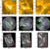 |
Fig. 1. Context of the ARs that generated the flares. The columns from left to right show the M4.6, C8.3, and M1.8 flares, respectively. The rows from top to bottom show the AIA 171 Å, Ca II 8542 Å core and Hβ core channels, respectively. Each panel show the flare near the GOES peak time, and the timestamps are shown in the lower right corners. The GOES X-ray plot is added in the lower left corner in the upper row, where the x axis is in minutes relative to the image. The red and cyan contours highlight the FOVs of CRISP and CHROMIS, respectively. The green and blue contours in the middle row show the CRISP magnetogram at ±500 G. The red boxes in the lower row correspond to the FOVs in Figs. 3–5, respectively. An animation of this figure is available online. |
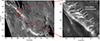 |
Fig. 2. Fine-scale structures or riblets in a flare ribbon located near the western limb in a complex photospheric magnetic field configuration (flare F1). The right panel is a smaller FOV, as highlighted by the red rectangle in the left panel, revealing the fine-scale structures in a ribbon from a side view. The colour maps in the left and right panels are in logarithmic and linear scales, respectively. |
Characteristics of each flare in the study.
2.2. Flare morphology
The three flares occurred in different active regions. Only AR 13376 (F1) had two sunspots with opposite polarities and developed the strongest flare in the list. While a single sunspot was evident in the two other ARs, strong magnetic fields were evident in the form of prominent flux concentrations in SST Fe I 6173 Å magnetograms. Each flare was associated with an erupting filament seen in AIA channels, with one end seemingly connected to a sunspot penumbra. Two ribbons connected above strong patches of opposite-directed polarity regions in the photosphere are evident for all three flares. For the F1 and F3 flares, the ribbons of opposite polarities were seemingly anti-parallel, resembling the characteristic ‘J-shape’ ribbon pair, indicated by the white arrows in Figs. 1g and 1i, respectively. The underlying opposite-directed magnetic field is visible in Figs. 1d and 1f by the green and blue contours. The F2 flare exhibits a pair of ribbons, but an anti-parallel configuration is not evident. The straight parts of the ribbons are nearly perpendicular relative to one another. Additionally, the ribbon closer to the sunspot lacks a well-defined hook. The evolution of each flare is presented in Fig. 1 (see also the associated animation in the online material). In the AIA 171 Å coronal channel, flare loops connecting the opposite polarity ribbons are visible (indicated by the black arrow in Fig. 1b). The flare loops from the F1 flare in Fig. 1a saturate the image.
2.3. Observing programmes and data reduction
The three flare events were observed with the CRisp Imaging SpectroPolarimeter (CRISP; Scharmer et al. 2008) and the CHROMospheric Imaging Spectrometer (CHROMIS; Scharmer 2017) installed at the Swedish 1-m Solar Telescope (SST; Scharmer et al. 2003). CRISP was running a programme similar to what is described in Paper I, sampling the Fe I 6173 Å and Ca II 8542 Å lines in spectropolarimetric mode. The F1 and F2 flares include the Hα line in spectral imaging mode. The field of view (FOV) of CRISP has a diameter 87″, which is larger than for the observations in Paper I. Here, we concentrate on the CHROMIS observations that sampled the Hβ line in 29 line positions between ±2.7 Å. The sampling steps were 0.1 Å in the core region between ±1 Å, and coarser (varying between 0.15−0.8 Å) in the wings to avoid spectral line blends. The cadence was about 11 s. CHROMIS had a pixel scale of about 0 038 and a FOV of about 72″ × 48″. The diffraction limit, λ/D, of the SST with its D = 0.97 m aperture is about 0
 1 at λ = 4861 Å. The data were processed following the standard SSTRED data reduction pipeline (de la Cruz Rodríguez et al. 2015; Löfdahl et al. 2021) which includes multi-object multi-frame blind deconvolution (MOMFBD; Van Noort et al. 2005) image restoration. We performed an AIA-to-SST alignment to add context to the AR associated with the respective flares. The AIA 171 Å channel provides insights into the magnetic configuration in the corona during the evolution of the flares.
3. Methods
3.1. k-means
To tackle the vast amount of data points, machine learning techniques were employed. We used k-means clustering to effectively group pixels into k clusters that represent a spectral profile with a unique shape (Everitt 1972). These groups are referred to as representative profiles (RPs). An optimised initialisation of each cluster centroid is based on the idea of Arthur & Vassilvitskii (2007), where new centroids are drawn far away from previous centroids in terms of Euclidean distance. This method has previously been proven to be a helpful tool for grouping large numbers of data points from different solar events into representative groups (see, e.g. Joshi & Rouppe van der Voort 2022; Testa et al. 2023; Sainz Dalda et al. 2024; Crowley et al. 2025). We utilised the open-source Scikit-learn package (Pedregosa et al. 2011). The learning procedure iteratively modifies the shape of the RP based on the number of pixels assigned to that particular RP cluster. We found that k = 100 for the F2 flare and k = 120 for the F1 and F3 flares were optimal for our analysis. A detailed explanation on determining k is provided in Appendix A.
Clustering all pixels from a dataset is excessive since the analysis is restricted to the fine-scale features in flare ribbons. Additionally, including all pixels for clustering could potentially omit rare but important RPs. For these reasons, a three-step masking routine was developed to confine the analysis to the ribbon areas. In the first step, we applied an intensity threshold to the integration over a few selected wavelengths in the line core region. In the second step, we manually removed pixel areas that were brighter than the intensity threshold but were located clearly outside the ribbon. This step was aided by the aligned AIA images. In the third step, we applied morphological erosion and dilation operations to slightly grow the masked areas to make sure all relevant pixels were included.
3.2. Identify fine structures in ribbons
We aim to identify fine structures in a ribbon that appear close in time to the GOES X-ray peaks. The identification process is performed using Hβ +0.8 Å wing images. In Paper I, we referred to these features as blobs due to their spatial periodicity and circular structures. Here, we refer to these features as riblets. An example of riblets is presented in Fig. 2. Pixels in Hβ +0.8 Å that are part of such structures were labelled, and the RPs associated with these pixels were tagged accordingly. We performed the identification step at a smaller FOV for multiple frames to ensure all relevant RPs were selected. If an RP was associated with an excessive portion of the ribbon that is not considered a riblet, we disregarded that particular RP from further analysis.
The RPs associated with riblets revealed that their spectral shapes are diverse. We organised the RPs in three subgroups based on their spectral properties. One subgroup is associated with RPs that consist of a single emission peak. The other two subgroups are associated with profiles with double emission peaks. They were segregated based on whether the red peak is stronger or if both peaks are equally strong. The subgroups allow us to distinguish between the different spectral characteristics along the flare ribbon.
3.3. Emission profile fitting
Flaring profiles are often recognised by their emission signatures that can be approximated to a Gaussian profile. All pixels associated with the blobs detected in Paper I show the Hβ line in emission. In this work, we used the labelled pixels from the k-means clustering and applied Gaussian fitting on individual pixels associated with a riblet to extract their spectral properties. The profiles were fitted to the following function:
 (1)
(1)
where I(λ) describes the intensity profile with respect to the wavelength λ, A is the amplitude of the profile, λ0 is the Doppler shift, σ is the standard deviation associated with the width of the profile, and d is a constant offset to account for the intensity levels at the far wings. Pixels that were associated with a double-peaked RP were fitted with a double-Gaussian function with one component for an emission line and the other for a superimposed absorption line. The fitted absorption line will mimic non-flaring material that blocks the radiation along the line of sight (LOS) of the telescope. We analysed the fitted emission line under the assumption that the ribbon fine structure will be in emission. If a pixel belongs to a single-peaked RP cluster, one Gaussian in emission was fitted. The distributions of the fitted parameters are presented in Sect. 4.3 and in Table 2.
Riblet statistics.
4. Results
4.1. Imaging overview of riblets
The impulsive phase is well covered for the F2 flare and the F3 flare observations, while the F1 flare was only covered from around the GOES peak time. The F2 and F3 flares indicate that the riblets form the ribbon fronts just before the GOES peak time. The collective pattern of riblets propagates along the ribbon during the progression of the flares until they fade. While the F3 flare shows clear signatures of riblets during the impulsive phase and during the peak time, riblets from the F2 flare seem to fade before reaching the GOES peak (see the animation associated with Fig. 1 available in the online material). The F1 riblets are evident near the time of the GOES peak and also show a collective motion along the ribbon. The motion of the ribbon fronts is not discernible from the F1 flare. All three observations show that the riblets jointly constitute the ribbon structure, clearly seen from the Hβ +0.8 Å images.
The F1 flare is the only observation close to the limb, and therefore provides a side view into the ribbons. Small-scale brightenings are evident within the ribbons showing the extension of the riblets, seen as bright streaks in Fig. 3b. The riblets evidently constitute an array of features that form the ribbon. The F1 flare indicates that the general structure of riblets comprises thin streaks that extend vertically upward from lower atmospheric heights, as they typically extend towards the limb. The estimated length and width of the riblets are provided in Table 2. Individual features appear to have footpoints that extend further down to a common, continuous structure that stretches parallel to the surface. The continuous structure does not vary much over time compared to the riblets. The larger feature at [X, Y]=[890″, 427″] does not exhibit a typical riblet structure, as its width is approximately equal to its length. Images at the Hβ core show that this feature could be a composition of smaller features, as is seen in Fig. 3d. The composition is supported by the colour map in Fig. 3c, as smaller confined features are more prominent in this map.
The k-means clustering effectively identified pixels that were associated with a riblet along the ribbons. All pixels categorised as a riblet were labelled accordingly and overplotted in Figs. 3a and 3d in colours for the limb flare. The colours associate the pixels with RPs that consist of different profile characteristics, as is explained in Sect. 3.2. The riblets show an overrepresentation of red-dominant double-peaked profiles. Hβ core images reveal that the central reversal of the profiles can be affected by the canopy blocking the LOS in the chromosphere. Symmetrical double-peaked profiles are less frequent and are located only at the riblet footpoints. The larger feature at [X, Y]=[890″, 427″] is mainly composed of single-peaked emission profiles and is not shadowed by the canopy, as can be seen from the Hβ core in Fig. 3d. The clustering by k-means effectively tags the riblets along the ribbon, depending on the spectral characteristics within the local area.
The fitted Doppler shifts and profile widths obtained from the main emission component are overplotted in Figs. 3e–f, respectively. The Doppler velocities at the body of the riblets are consistently higher than the footpoints. A thorough investigation of the blueshifted pixels was deemed unreliable, as the fitted profiles deviate too much from the data. These pixels exhibit a correspondence with a stronger offset in the blue wing at Hβ −0.8 Å, as can be seen from the colour map in Fig. 3c. The widths of the profiles, as is seen in Fig. 3f, suggest that the riblet bodies consist of narrow emission profiles while the footpoints have comparably broad profiles.
The weaker F2 flare exhibits less prominent riblet signatures, although they were detected as part of the ribbon structure. The results from k-means showed that about 40% of the pixels labelled as a riblet were categorised as a single-peaked emission profile, and about 60% are related to a double-peaked profile. The locations of the riblets are highlighted by the coloured pixels in Figs. 4a and 4d, where the latter shows that the riblets are part of the ribbon front. The coloured pixels show that both single-peaked and double-peaked profiles are evident along the ribbon front. This combination may be caused by projection effects, as the conjugate ribbon is located closer towards the limb, causing some of the pixels to be shadowed by material in the LOS. The estimated Doppler velocities are consistently towards the red. Stronger redshifts are located near regions where signatures of enhanced photospheric magnetic fields are evident, seen as pores; for example, at [X, Y]=[−628″, −212″] and [X, Y]=[−620″, −224″] in Fig. 4e. The estimated profile amplitudes are also more significant closer to the pores.
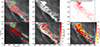 |
Fig. 3. Riblets along the F1 ribbon. All panels show the same FOV, highlighting the central parts of the eastern ribbon. All panels except panels c–d show images in the Hβ +0.8 Å channel. Panel c shows the wing-subtracted colour map at Hβ ± 0.8 Å. Panel a shows the ribbon with identified riblets overplotted in green, red, or cyan. Green pixels represent single-peaked RPs, red pixels represent double-peaked RPs with a stronger red peak, and cyan pixels represent near-symmetric double-peaked RPs. Similar is shown in panel d overplotted on the Hβ core image. The resulting Doppler shifts and profile widths obtained from fitting the pixels are shown in panels e–f, respectively. The black pixels in panel e mask the pixels where blue shifts were estimated. The contours of these pixels are added in panel c. An animation related to this figure is available online. |
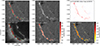 |
Fig. 4. Same as Fig. 3 but for the F2 flare. The superimposed pixels in panel f are replaced with the estimated amplitude, A, from profile fitting. An animation related to this figure is available online. |
The results of the k-means algorithm applied to the F3 DC flare show that the majority of riblets are related to single-peaked RPs, as is overplotted in green in Figs. 5a and 5d. The coloured pixels are located along the ribbon front that is propagating to the west. Double-peaked profiles are evident in areas where chromospheric material is enveloping the ribbon, and can be seen as red pixels at [X, Y]=[152″, 128″] in Fig. 5d. The parameters from the fitting indicate that stronger redshifts, λ0, are located at the ribbon fronts, similar to those in the F2 flare. The estimated Doppler velocity range is shown in Table 2. The strongest profiles in terms of amplitude, A, are located above pores in the photosphere, as is seen by the dark underlying structure in Fig. 5f. The pores are associated with strong negative magnetic fields close to an opposite and near equally strong region to the east, as is seen near [X, Y]=[152″, 133″] in Fig. 1f.
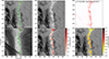 |
Fig. 5. Same as Fig. 3 but for the F3 flare. The overplotted colours in panel f are replaced with the estimated amplitude, A, from profile fitting. An animation related to this figure is available online. |
4.2. Spectral characteristics of riblets
The k-means effectively clustered the spectral profiles into categorical shapes for each dataset. The observations captured the three flares at different viewing angles, μ, which provides an augmented analysis. The spectral properties of the riblets show a clear signature in emission, but different compositions of the spectral properties were discerned. Here we show the results of the RPs obtained from the k-means clustering, and present the spectral characteristics from the three observational datasets.
The RPs obtained from the k-means clustering of the F1 limb flare generated mainly double-peaked RPs. The RPs from the F1 flare riblets are shown in Fig. 6. The coloured distribution in each panel is well aligned with the associated RP. The single-peaked RP 0–2 peaks are redshifted with evident broadening of the profiles. The green density distributions show that there is a systematic redshift of basically all the profiles in these clusters. The structures of RP 3–6 are nearly symmetric with excessive broadening. A significant RP wing enhancement is not evident on either side. RP 7–16 represent double-peaked profiles with a stronger red peak, which are the most common types for the limb observation. Excessive profile broadening is common for these RPs. RPs with prominent enhanced red wings are common except for RP 7, RP 11, and RP 15. A clear indication from the RPs and the associated observed profiles shows that riblets consist of an emission component.
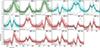 |
Fig. 6. Hβ spectral profiles associated with riblets from k-means clustering of the F1 flare. Solid black lines show the RPs with the identity labelled in the upper right corner, and the coloured background shows the density distribution of all the clustered profiles. Denser distribution is shown in a darker colour. The dotted black line is the profile furthest away from the RP in Euclidean distance. For reference, the solid grey line is the average profile from a QS region. All profiles are normalised by the far blue wing of the average QS profile. The green distributions are associated with apparent single-peaked RPs, cyan distributions are associated with double-peaked and near-symmetric RPs, and the red distributions are associated with double-peaked RPs with a stronger red peak. The parameter n in all panels represents the fraction of each cluster to the total number of pixels in all timeframes used for clustering. The total number of masked pixels used for clustering was ∼7.8 × 10⁶. |
The RPs associated with the F2 flare riblets are generally weaker than the RPs obtained from the F1 flare. The peak amplitudes are typically near or below A = 2 in normalised units, except for RP 9, which has an amplitude of 2.4, seen in Fig. 7. Some of the individual profiles in this cluster have a peak amplitude above 2.7. The distribution of pixels within single-peaked RP clusters aligns well with the corresponding RP, and both suggest redshifts, as is shown by the black line and the green distribution, respectively, in RP 0–3. Only one near-symmetric and double-peaked RP was obtained (RP 4). RP 5–12 are associated with double-peak profiles, with a stronger red peak. There is no signature of a prominent blue peak in any of RP 5–12. The red peak is significantly stronger than the blue peak for RPs 6, 7, 9, 11, and 12. The RPs obtained from the F2 flare show that riblets closer to DC (μ = 0.79) than the F1 flare are still significantly prone to central reversal signatures.
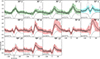 |
Fig. 7. Same as Fig. 6 but for the F2 flare. A total of ∼6.8 × 106 pixels were used for the k-means clustering. |
The F3 DC flare observation has more single-peaked RPs than the other two flares (see Fig. 8). All the RPs show a redshifted trend with variable profile amplitudes. The density distribution fits well with the RPs. The variation in the distributions seems to be stronger near the peaks of the RPs and more prominent for the stronger profiles, as is seen by comparing RP 3 with RP 8. RP 14–18 has a double-peaked signature with a stronger red peak, although the blue peak in RP 16 and RP 17 is small. The shape of all the red-coloured profiles suggests redshifts. For all RPs, a red wing enhancement is not a consistent feature. Blue wing enhancements can be discerned from the density distributions; for example, from RP 12 and the dotted line in RP 15.
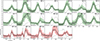 |
Fig. 8. Same as Fig. 6 but for the F3 flare. A total of ∼12.3 × 106 pixels were used for the k-means clustering. |
4.3. Outcome of profile fitting
In this section, we present the properties extracted from profile fitting associated with the riblets. Each pixel was fitted to a single or double-Gaussian curve, based on the category it was labelled to by the k-means algorithm. Note that some single-peaked pixels were categorised as double-peaked from the k-means clustering, and vice versa. Such false categorisation is likely due to the vast complexity of flaring profiles, suggesting that the number of clusters, k, could be increased. Increasing the number of clusters implies an excessive number of RPs. Although misplacement of pixels is inevitable for the chosen number of clusters, k, the fitted emission component is still sufficiently representative of the observed profile. At least, for statistical significance purposes, when estimating the properties of riblets.
Double-peaked profiles are naturally more complex than single-peaked profiles. By visually inspecting the goodness of the fit on the double-peaked profiles, it was concluded that the procedure struggled in many cases to capture both the main emission component and the central reversal component sufficiently. For instance, instead of capturing the full profile width, the fitting procedure evaluated only the red peak, which yielded inaccurate parameter estimates. This issue led to the exclusion of pixels labelled as double-peaked when interpreting the evolution of the fitted parameters in Fig. 9.
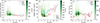 |
Fig. 9. F3 riblet evolution of the parameters obtained from the profiles fitted to a single Gaussian curve. The distributions show the fitted amplitude, Doppler shifts, and broadening from (a)–(c), respectively. In all panels, the green background represents the distribution with respect to time. The mode, mean, and median of each distribution per timestep are shown as red, cyan, and pink curves, respectively. The white columns represent frames that were disregarded due to worse seeing. Bins with a contribution less than 1/100 of the maximum bin are coloured in white. The two short vertical black lines at Δt = 3.4 min mark the timestep with the highest number of pixels identified as riblets. The distribution of the fitted parameters of this timestep is shown in Fig. 10. |
The amplitude, Doppler shifts, and profile widths were determined by the distribution of the fitted parameters, providing a statistical estimate of the properties associated with riblets. The results of the distribution from the F3 flare are presented in Fig. 9, which shows how the properties evolve over time from a top-view perspective. Only the pixels fitted to a single Gaussian curve were analysed. A clear transition of the increased number of riblets occurs at Δt = 2 min, which is during the impulsive phase. The distribution at this timestep is the most spread, showing peaks above A = 4.0. The amplitudes of the mode, mean, and median curves are nearly equal to A ∼ 2.5 at Δt = 2 min. A descending trend is evident for the mean and median curves until the riblets completely fade at around Δt = 8 min, dropping below A < 2.3. A descending trend is also evident for the Doppler shift but for a shorter time range, from Δt = 2 − 4.5 min. The mean and median curves are more correlated, starting at λ0 ∼ 35 km s−1 to λ0 ∼ 25 km s−1. A consistent offset of about −10 km s−1 is evident between the mode curve and both the mean and median curve. The highest density of the fitted widths is approximately constant at σ ∼ 33 km s−1, except between Δt = 2 − 3 min, where the density distributions and the mode curve indicate a trend of increasing widths.
We present the performance of the double-Gaussian fit by comparing its results with the single-Gaussian fit. The results from the F3 DC flare riblets are presented in Fig. 10 at the timestep where most pixels were labelled as a riblet at Δt = 3.4 min, just before the GOES peak. There is an offset between the peaks of the amplitude distributions, indicating that double-Gaussian profiles are more related to stronger profiles. The Doppler shift distribution for the single-peaked profiles has a valley near 22 km s−1, seen by the green bars in Fig. 10b. The gap shows a correlation with the peak of the double-Gaussian distributions, seen by the red bars in the same panel. The distributions of the widths are fairly similar, except that the distribution for the double-Gaussian fit shows an extra peak at σ ∼ 43 km s−1. For all three parameters, the cumulative of both single-Gaussian and double-Gaussian forms a relatively smooth curve, as is seen by the black line in all panels in Fig. 10. The cumulative amplitude and Doppler shift curves show a sharp transition before the curve peak and a wider spread after the peak. The estimated profile widths are nearly symmetric around the peak.
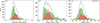 |
Fig. 10. Distribution of the fitted parameters obtained from the F3 flare riblets at Δt = 3.4 min just before the GOES peak. This is the timestep with the highest number of pixels identified as riblets. The green bars show the distribution of fitting to a single Gaussian curve. The red bars represent the distribution of parameters obtained from the main emission component of the double-Gaussian fitted profiles. The black curve is the cumulative of the green and red bars. |
4.4. Statistical properties of riblets
The statistically significant properties of the riblets are presented in this section from an imaging and a spectral point of view. Section 4.1 presents images of the riblets at different viewing angles, showing that riblets near the limb are prone to being obscured around the Hβ line core by intervening chromospheric material, unrelated to the flare, along the LOS. This affected the results of the k-means clustering such that more RPs were categorised as double-peaked, and the number of pixels belonging to this category was favoured. The number of RPs associated with the single-peak or double-peaked category is presented in the first row in Table 2. The fraction of riblet pixels that have a single or double peak is presented in the second row. The table shows that a significant number of pixels are categorised as double-Gaussian closer to the limb, with a decreasing trend towards the DC, from 92% to 26%. The DC observation is less prone to intervening material, although chromospheric material is periodically flowing above the ribbons, as is seen by the dark feature centred at [X, Y]=[150″, 130″] in Fig. 5d. Such material flows reflect on the spectral profiles forming a central reversal component and tag the related pixels as double-peaked, as is seen by the red pixels in Fig. 5d near [X, Y]=[152″, 128″].
We measured the lengths and widths of a selection of prominent riblets from each dataset. The measurements were computed based on the full width at half maximum (FWHM) of their spatial intensity profile in the Hβ +0.8 Å wing, which provides a rough estimate of their sizes. We refer to Paper I for a detailed explanation of how the measurements were performed. The estimated range of lengths and widths is provided in Table 2. Assuming that riblets are vertical relative to the surface and accounting for projection effects, the measured length of 580−1500 km implies a vertical extent of approximately 620−1590 km for the μ = 0.35 limb flare. The lengths from the μ = 0.79 flare measured at 280−750 km imply a vertical extent of approximately 460−1220 km, indicating that the riblets are shorter for this flare. We consider that the riblets follow the magnetic field towards coronal heights, implying that the riblets are nearly vertically oriented. We consider two additional cases, assuming an offset of 30 and 45° from the vertical. For the F1 flare, the length ranges are 760−2000 km and 640−1700 km, respectively. For the F2 flare, the estimated riblet length ranges are 280−760 km for both offsets. No lengths for the riblets near DC were measured. The widths are consistent for all three flares.
Measures of the range of values obtained from the spectral profile fitting are presented in the bottom three rows of Table 2. We present the maximum and minimum of the FWHM of the parameter distributions. The amplitudes from the three flares show a correlation with the measured X-ray levels from GOES; that is, the F1 flare (M4.6) has a higher range of amplitudes, while the F2 flare (C8.3) has a lower range. The ranges do not overlap between these two observations. The M1.8 flare (F3) has a distribution between these two distributions. The overlapping Doppler velocities between the observations range from 16−21 km s−1, but the extremums do not show a clear sign of correlation between the characteristics from each flare. The strongest Doppler shift within the FWHM interval is measured to 44 km s−1 for the μ = 0.79 flare. This flare is associated with the narrowest profiles, as the lower limit of the line width is estimated at 12 km s−1. The maximum line width of the DC μ = 0.98 flare is lower than that of the other flares. The acquired ranges presented in Table 2 suggest a correlation between the fitted amplitudes and the strength of the flare, while a correlation between the strength and the fitted shifts or line widths is not evident. However, any possible correlation needs to be checked with a larger, statistically significant sample.
5. Discussion
As an extension of our Paper I, this detailed study reveals, through colour mapping of the observed flares, that the fine structures form the leading edges of the ribbons. Using He I 10830 Å Xu et al. (2016) found that ribbon fronts could be as narrow as 340 km wide, which is consistent with our results presented in Table 2. Naus et al. (2022) found that the front widths along the ribbon are irregular in space and time, varying from 0.6−1.2 Mm, which is greater than the widths of our riblets. The width of the riblets is indeed irregular along the ribbon, although we found the widths to be less than 600 km. The width of the riblets in Hβ +0.8 Å may not necessarily explain the full width of the ribbon fronts, but rather probe the precise location of the ribbon front footpoints, as the material at the footpoints is more illuminated.
In Paper I, we found a distinct periodicity between the blobs with separation distances ranging from 330−550 km. Using similar methods, we found that the distances have an overlapping range of 200−280 km in our current analysis. Plausible evidence of tearing is based on the presence of conjugate ribbons, which are found in all three observations, in addition to the riblets that are evident in both conjugates in all three flares. We support the idea that fine-structure periodicities are related to current sheet dynamics (Dahlin et al. 2025) that are possibly due to tearing of small-scale flux ropes (Wyper & Pontin 2021). Discerning similar periodicity was identified from the F1 limb flare, which can be seen in Fig. 3b as the riblets are near equidistant. Although comparable periodicities are evident between the F1 riblets and the blobs in Paper I, the variation in size between neighbouring riblets is more prominent in the F1 flare. In numerical modelling, the relative sizes of these types of fine structures have not yet been clearly inferred. Given that the riblets are formed due to reconnection in the current sheet, it is not clear if the variation in size is caused by irregularities at the reconnection site or if there is significant interaction in the plasma during the transport of energy from the current sheet to the riblets. It seems that the energy transport interaction is less evident for the weaker flare in Paper I, which resulted in the formation of near-equidistant blobs with nearly equal widths.
The number of pixels associated with riblets from all three observations is abundant. Many of the spectral profiles from these pixels show complex emission properties, which leads to relatively unique RPs from the k-means clustering. A selection of complex profiles is shown as the most distant profiles in all panels in Figs. 6, 7, and 8. For instance, the distant profile in cluster RP 0 in Fig. 6 is double-peaked and broadens beyond the spectral window, but was identified in a single-peaked RP cluster. Another example is RP 1 in Fig. 7: the distant profile seems skewed towards the red, and the blue wing is weaker than the QS average. The distant profile in RP 18 in Fig. 8 shows a blueshifted emission profile where the peak has a plateau-like shape. These examples of highly complex profiles, among others within the datasets, demonstrate that the fine structures in a flare ribbon generate intricate and diverse emission profiles. Although such profile shapes are rare, the most deviant profiles suggest that increasing the number of clusters could be considered to sufficiently capture these profiles and produce RPs that are more similar in shape. On the contrary, analysing a larger number of RP would be time-consuming and inefficient. We argue that it is sufficient to train a k-means model with k = 100 and k = 120 for C-class or M-class flares, respectively.
We categorised the riblets based on the profile shape into two main categories: single-peaked and double-peaked. Both categories were detected in all three flare observations, but the trend indicates that the occurrence rate of single-peaked profiles is increasing from limb to DC. The double-peaked profiles are generally characterised by a stronger red peak. The shifts of the central reversals were < 5 km s−1 for the F2 and F3 DC riblets and around 0 km s−1 for the F1 limb riblets. Assuming the riblets to be the footpoints of magnetic loops and that plasma is accelerated downwards from the current sheet, redshifted profiles are more prominent when the magnetic fields are aligned with the LOS, which explains why the central reversal is more redshifted for the F3 DC observation (Compare, for example, RP 7–16 in Fig. 6 with RP 14–18 in Fig. 8). Since detailed information about the magnetic field geometry is unknown and there is an increased chance of an absorption component at more inclined viewing angles, the question of whether the Doppler offset of the main emission component in the F1 limb profiles can be interpreted as a clean measurement of the plasma velocity remains uncertain. However, we note that red-dominant profiles in the chromosphere are not necessarily a sign of downflows, since a blueshifted absorption component can produce a redshifted emission profile (Kuridze et al. 2015; Yadav et al. 2025). Nevertheless, we argue that the observed riblets are part of magnetic loops extending in the corona, consistent with tearing-mode theories (Wyper & Pontin 2021; Dahlin et al. 2025). Hence, we interpret the redshifts as plasma downflows. Images in Hβ core channel from the three flares reveal that the chance of structures in the chromosphere blocking the LOS of riblets is increasing towards the limb, which causes more double-peaked profiles to be formed. The chromospheric canopy in the F1 limb observation is dense enough to block a significant amount of the radiation from the riblets (see transparent red pixels in Fig. 3d). Only the strongest feature at [X, Y]=[890″, 427″] penetrates the canopy. The riblets from the F3 flare are mostly associated with single-peaked profiles, as is seen by the transparent green pixels in Fig. 5d. Double-peaked profiles in red are indeed evident at [X, Y]=[152″, 128″] and are blended by chromospheric material overarching the riblets. Therefore, the spectral properties of ribbon fine structures are likely always in full emission and blocked by overlying material when observed with two peaks.
Very recently, Yadav et al. (2025) analysed ribbon fine-scale structures using the Daniel K. Inouye Solar Telescope (DKIST; Rimmele et al. 2020), which show similar spatial properties of the blobs as in our Paper I. They found that the Ca II 8542 Å lines of the blobs exhibit double-peaked profiles, which is contrary to Paper I that only showed single-peaked profiles. The study presented here, based on three flares occurring at different positions on the solar disc, suggests that the formation of double-peaked chromospheric profiles is more likely at larger distances from the DC, as is exemplified by the limb-near flare in Yadav et al. (2025).
The fitting of double-peaked profiles was challenging due to the diverse complexity of these profiles. Therefore, these pixels need to be carefully analysed when interpreted, preferably as a standalone analysis of these particular pixels. The fitting of individual pixels associated with a riblet enabled us to construct an overview of the plasma dynamics by overplotting the fitted parameters on top of the images. In Fig. 3e, we show the fitted Doppler velocities of the F1 flare. We emphasise that the riblets are observed with a significant inclination angle, indicating that the velocities perpendicular to the surface may be higher. The body of the riblets is mainly redshifted. The redshifts are apparently trending towards 0 km s−1 closer to the footpoints. A correlation with the line widths can be discerned, as the riblet bodies generally show narrower widths, and the footpoint widths are excessive (Fig. 3f). It appears that the plasma is decelerated along the riblet structures and brakes near the footpoint. This potential velocity gradient seems to be associated with line widths, as the widths are broader at the riblet footpoints.
The riblets from the F2 and F3 flares were observed from a top view, which prevents identifying the body and footpoints of the riblets. The fitted Doppler shifts are seen in Figs. 4e and 5e, obtained from the F2 and F3 flares, respectively, which show that the riblets are generally covered by redshifted pixels. Since the footpoints of the riblets are not evident, a change in Doppler velocity from the riblet body to the footpoint is not evident. Both F2 and F3 exhibit a potential correlation between strong profiles and pores in the photosphere. This is seen in Figs. 4f and 5f for F2 and F3, respectively. The prior shows a patch of dark pixels, representing strong profiles, near [X, Y]=[−630″, −213″], which is adjacent to a photospheric pore. A similar signature is observed in the latter figure, near [X, Y]=[152″, 133″], where strong profiles are overlapping the underlying pores. Pores in the photosphere are formed due to high magnetic density, which implies that the formation of stronger Hβ flare profiles may be associated with regions where underlying strong magnetic fields are present.
6. Conclusions
Based on high-resolution SST observations of three solar flares, we conclude that flare ribbons consist of extremely fine structures (or blobs) when viewed close to the solar limb. These structures were identified as riblets, according to the definition first introduced by Singh et al. (2025). Riblets are elongated fine structures that form the ribbon fronts. These features were detected in all three flares, which complements the previous detection of ribbon fine structure from ground-based observations (Brannon et al. 2015; French et al. 2021; Singh et al. 2025) and the more recent observations with DKIST (Yadav et al. 2025). We suggest that such a fine structure might be common in flare ribbons, but a comprehensive statistical analysis is needed to confidently establish the ubiquity of ribbon fine structure in all C-class flares and stronger.
In our analysis, it becomes evident that the analysed flare ribbons are composed of arranged small-scale features – riblets – and are not a continuous structure. As the ribbons constitute the footpoints of reconnection loops that extend into the corona, the array of fine structures along the ribbon suggests that the reconnection process in the solar corona is fragmented. The fragmentation is likely associated with the formation of magnetic islands in the current sheet, although this has not been directly observed. The ribbon fine structures comprise observational evidence that supports the theoretical idea of tearing in the flare current sheet or the patchy reconnection.
The spectral shapes of riblets are mainly redshifted emission profiles. The profile shapes from the blobs in Paper I are of a similar nature, with redshifted emission profiles, and are consistent with this statistical analysis. Double-peaked profiles are likely produced by an absorption component due to the presence of material above the Hβ formation height along the LOS.
In this way, high-resolution observations are essential for advancing our understanding of fine-scale solar flare dynamics. The recently published catalogue of 19 solar flares observed with the SST by De Wilde et al. (2025) offers a valuable resource for such studies. Looking ahead, we anticipate further insights from upcoming observations by DKIST, Solar Orbiter (Müller et al. 2020), and the European Solar Telescope (EST; Quintero Noda et al. 2022).
Data availability
Movies associated with Figs. 1, 3 – 5 are available at https://www.aanda.org
Acknowledgments
We wish to thank the referee for their valuable comments, which improved this paper. We acknowledge our fruitful discussions with G. Aulanier, L. Fletcher, and H. Hudson. We thank S. Tønnessen for assistance with the observations. This research is supported by the Research Council of Norway, project number 325491, through its Centres of Excellence scheme, project number 262622. The Swedish 1-m Solar Telescope (SST) is operated on the island of La Palma by the institute for Solar Physics of Stockholm University in the Spanish Observatorio del Roque de los Muchachos of the Institutio de Astrofisica de Canarias. The SST is co-funded by the Swedish Research Council as a national research infrastructure (registration number 4.3-2021-00169).
References
- Acton, L. W., Leibacher, J. W., Canfield, R. C., et al. 1982, ApJ, 263, 409 [Google Scholar]
- Arthur, D., & Vassilvitskii, S. 2007, Proceedings of the Eighteenth Annual ACM-SIAM Symposium on Discrete Algorithms, SODA ’07, 1027 [Google Scholar]
- Aulanier, G., Janvier, M., & Schmieder, B. 2012, A&A, 543, A110 [NASA ADS] [CrossRef] [EDP Sciences] [Google Scholar]
- Benz, A. O. 2008, Liv. Rev. Sol. Phys., 5, 1 [Google Scholar]
- Brannon, S. R., Longcope, D. W., & Qiu, J. 2015, ApJ, 810, 4 [NASA ADS] [CrossRef] [Google Scholar]
- Carmichael, H. 1964, NASA Spec. Publ., 50, 451 [NASA ADS] [Google Scholar]
- Chandra, R., Schmieder, B., Aulanier, G., & Malherbe, J. M. 2009, Sol. Phys., 258, 53 [Google Scholar]
- Crowley, J. W., Milić, I., Cauzzi, G., & Reardon, K. 2025, ApJ, 986, 124 [Google Scholar]
- Dahlin, J. T., Antiochos, S. K., Wyper, P. F., Qiu, J., & DeVore, C. R. 2025, ApJ, 993, 31 [Google Scholar]
- de la Cruz Rodríguez, J., Löfdahl, M. G., Sütterlin, P., Hillberg, T., & Rouppe van der Voort, L. 2015, A&A, 573, A40 [NASA ADS] [CrossRef] [EDP Sciences] [Google Scholar]
- De Pontieu, B., Title, A. M., Lemen, J. R., et al. 2014, Sol. Phys., 289, 2733 [Google Scholar]
- De Wilde, M., Pietrow, A. G. M., Druett, M. K., et al. 2025, A&A, 700, A275 [NASA ADS] [CrossRef] [EDP Sciences] [Google Scholar]
- Devi, P., Joshi, B., Chandra, R., et al. 2020, Sol. Phys., 295, 75 [NASA ADS] [CrossRef] [Google Scholar]
- Everitt, B. S. 1972, Br. J. Psychiatry, 120, 143 [Google Scholar]
- Fletcher, L., Dennis, B. R., Hudson, H. S., et al. 2011, Space Sci. Rev., 159, 19 [Google Scholar]
- French, R. J., Matthews, S. A., Jonathan Rae, I., & Smith, A. W. 2021, ApJ, 922, 117 [NASA ADS] [CrossRef] [Google Scholar]
- Hirayama, T. 1974, Sol. Phys., 34, 323 [Google Scholar]
- Jing, J., Xu, Y., Cao, W., et al. 2016, Sci. Rep., 6, 24319 [NASA ADS] [CrossRef] [Google Scholar]
- Joshi, J., & Rouppe van der Voort, L. H. M. 2022, A&A, 664, A72 [NASA ADS] [CrossRef] [EDP Sciences] [Google Scholar]
- Joshi, R., Aulanier, G., Radcliffe, A., et al. 2024, A&A, 687, A172 [NASA ADS] [CrossRef] [EDP Sciences] [Google Scholar]
- Joshi, R., Dudík, J., Schmieder, B., Aulanier, G., & Chandra, R. 2025, A&A, 698, A301 [NASA ADS] [CrossRef] [EDP Sciences] [Google Scholar]
- Kerr, G. S., Xu, Y., Allred, J. C., et al. 2021, ApJ, 912, 153 [NASA ADS] [CrossRef] [Google Scholar]
- Kopp, R. A., & Pneuman, G. W. 1976, Sol. Phys., 50, 85 [Google Scholar]
- Kuridze, D., Mathioudakis, M., Simões, P. J. A., et al. 2015, ApJ, 813, 125 [Google Scholar]
- Lemen, J. R., Title, A. M., Akin, D. J., et al. 2012, Sol. Phys., 275, 17 [Google Scholar]
- Löfdahl, M. G., Hillberg, T., de la Cruz Rodríguez, J., et al. 2021, A&A, 653, A68 [Google Scholar]
- Lörinčík, J., Dudík, J., & Polito, V. 2022, ApJ, 934, 80 [CrossRef] [Google Scholar]
- Masuda, S., Kosugi, T., Hara, H., Tsuneta, S., & Ogawara, Y. 1994, Nature, 371, 495 [CrossRef] [Google Scholar]
- Müller, D., St. Cyr, O. C., Zouganelis, I., et al. 2020, A&A, 642, A1 [Google Scholar]
- Naus, S. J., Qiu, J., DeVore, C. R., et al. 2022, ApJ, 926, 218 [CrossRef] [Google Scholar]
- Pedregosa, F., Varoquaux, G., Gramfort, A., et al. 2011, J. Mach. Learn. Res., 12, 2825 [Google Scholar]
- Pesnell, W. D., Thompson, B. J., & Chamberlin, P. C. 2012, Sol. Phys., 275, 3 [Google Scholar]
- Pietrow, A. G. M., Druett, M. K., & Singh, V. 2024, A&A, 685, A137 [NASA ADS] [CrossRef] [EDP Sciences] [Google Scholar]
- Quintero Noda, C., Schlichenmaier, R., Bellot Rubio, L. R., et al. 2022, A&A, 666, A21 [NASA ADS] [CrossRef] [EDP Sciences] [Google Scholar]
- Rimmele, T. R., Warner, M., Keil, S. L., et al. 2020, Sol. Phys., 295, 172 [Google Scholar]
- Rousseeuw, P. J. 1987, J. Comput. Appl. Math., 20, 53 [Google Scholar]
- Russell, A. J. B., & Stackhouse, D. J. 2013, A&A, 558, A76 [NASA ADS] [CrossRef] [EDP Sciences] [Google Scholar]
- Sainz Dalda, A., Agrawal, A., De Pontieu, B., & Gošić, M. 2024, ApJS, 271, 24 [Google Scholar]
- Scharmer, G. 2017, SOLARNET IV: The Physics of the Sun from the Interior to the Outer Atmosphere, 85 [Google Scholar]
- Scharmer, G. B., Bjelksjo, K., Korhonen, T. K., Lindberg, B., & Petterson, B. 2003, SPIE Conf. Ser., 4853, 341 [NASA ADS] [Google Scholar]
- Scharmer, G. B., Narayan, G., Hillberg, T., et al. 2008, ApJ, 689, L69 [Google Scholar]
- Schmieder, B., Forbes, T. G., Malherbe, J. M., & Machado, M. E. 1987, ApJ, 317, 956 [Google Scholar]
- Sharykin, I. N., & Kosovichev, A. G. 2014, ApJ, 788, L18 [NASA ADS] [CrossRef] [Google Scholar]
- Shibata, K., & Magara, T. 2011, Liv. Rev. Sol. Phys., 8, 6 [Google Scholar]
- Singh, V., Scullion, E., Botha, G. J. J., et al. 2025, ArXiv e-prints [arXiv:2507.01169] [Google Scholar]
- Sturrock, P. A. 1966, Nature, 211, 695 [Google Scholar]
- Testa, P., Bakke, H., Rouppe van der Voort, L., & De Pontieu, B. 2023, ApJ, 956, 85 [Google Scholar]
- Thoen Faber, J., Joshi, R., Rouppe van der Voort, L., et al. 2025, A&A, 693, A8 [NASA ADS] [CrossRef] [EDP Sciences] [Google Scholar]
- Van Noort, M., Rouppe van der Voort, L., & Löfdahl, M. G. 2005, Sol. Phys., 228, 191 [Google Scholar]
- Warren, H. P. 2000, ApJ, 536, L105 [NASA ADS] [CrossRef] [Google Scholar]
- Wyper, P. F., & Pontin, D. I. 2021, ApJ, 920, 102 [NASA ADS] [CrossRef] [Google Scholar]
- Xu, Y., Cao, W., Ding, M., et al. 2016, ApJ, 819, 89 [Google Scholar]
- Yadav, R., Kazachenko, M. D., Cauzzi, G., et al. 2025, ApJ, 989, 183 [Google Scholar]
- Yang, K., Guo, Y., & Ding, M. D. 2015, ApJ, 806, 171 [Google Scholar]
- Zuccarello, F. P., Chandra, R., Schmieder, B., Aulanier, G., & Joshi, R. 2017, A&A, 601, A26 [NASA ADS] [CrossRef] [EDP Sciences] [Google Scholar]
Appendix A: Evaluating the number of clusters
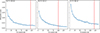 |
Fig. A.1. Silhouette score from the k-means algorithm. Each panel corresponds to the different flares with an increasing number of clusters, as denoted by the panel titles. For every iteration, a new subset of 25 000 random data points was used to compute the scores. The red vertical line in all panels denotes the number of clusters that were chosen for each dataset. |
We computed the silhouette score to decide the optimal number of clusters for each of the flares in the analysis (Rousseeuw 1987). The silhouette score ranges from -1 to 1. A score of 0 implies that the data points are located at the boundary between two clusters. A score close to 1 implies that the data points are relatively distant from neighbouring clusters, while a score close to -1 implies that the data point may have a better fit in another cluster. In our analysis, many spectral lines are relatively similar. The similarities between spectral lines are projected in the score plot in the sense that the silhouette score is consistently decreasing with increasing value of k, as is seen in Fig. A.1. Therefore, we conclude that the optimal silhouette score is where the curve flattens, which occurs approximately at k = 100, with scores of 0.13, 0.12, and 0.15 for the F1, F2, and F3 flares, respectively. See the red vertical line in Fig. A.1b. The next step involved checking if the clustering effectively captured the pixels associated with a riblet. This process was done by iterating through the clusters and highlighting the related pixels on the Hβ +0.8 Å images. The clusters highlighting a riblet were identified. We noted that during this step for the F1 and F3 flare, some riblet-related clusters included a significant amount of pixels that were not considered as riblets. Additionally, when inspecting the most distant data point from the cluster centroid in terms of Euclidean distance, more variation in the profile shapes was evident, which may exclude profiles of interest. We approached this issue by increasing the number of clusters to k = 120 for these two flares, which improved the accuracy of clustering the riblet-related pixels.
Appendix B: Spectral properties from limb and low viewing angle observation
The clustering of the F1 and F2 flare pixels resulted in an abundant representation of double-peaked profiles. We concluded in Sect. 4.3 that the fitting procedure did not reliably capture the main emission component and the central reversal component in many cases. Therefore, we do not include the parameter distribution figures in the main body of the article. For completeness, we present the figures in the appendix.
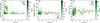 |
Fig. B.1. Same as Fig. 9 but for the F1 (μ = 0.35) flare. The figure shows the results only from pixels fitted to a single Gaussian curve. |
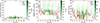 |
Fig. B.2. Same as Fig. 9 but for the F2 (μ = 0.79) flare. The results include only pixels that were fitted to a single Gaussian curve. |
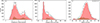 |
Fig. B.3. Same as Fig. 10 but for the F1 (μ = 0.35) flare. The results include only pixels that were fitted to a single Gaussian curve. |
All Tables
All Figures
|
Fig. 1. Context of the ARs that generated the flares. The columns from left to right show the M4.6, C8.3, and M1.8 flares, respectively. The rows from top to bottom show the AIA 171 Å, Ca II 8542 Å core and Hβ core channels, respectively. Each panel show the flare near the GOES peak time, and the timestamps are shown in the lower right corners. The GOES X-ray plot is added in the lower left corner in the upper row, where the x axis is in minutes relative to the image. The red and cyan contours highlight the FOVs of CRISP and CHROMIS, respectively. The green and blue contours in the middle row show the CRISP magnetogram at ±500 G. The red boxes in the lower row correspond to the FOVs in Figs. 3–5, respectively. An animation of this figure is available online. |
| In the text | |
|
Fig. 2. Fine-scale structures or riblets in a flare ribbon located near the western limb in a complex photospheric magnetic field configuration (flare F1). The right panel is a smaller FOV, as highlighted by the red rectangle in the left panel, revealing the fine-scale structures in a ribbon from a side view. The colour maps in the left and right panels are in logarithmic and linear scales, respectively. |
| In the text | |
|
Fig. 3. Riblets along the F1 ribbon. All panels show the same FOV, highlighting the central parts of the eastern ribbon. All panels except panels c–d show images in the Hβ +0.8 Å channel. Panel c shows the wing-subtracted colour map at Hβ ± 0.8 Å. Panel a shows the ribbon with identified riblets overplotted in green, red, or cyan. Green pixels represent single-peaked RPs, red pixels represent double-peaked RPs with a stronger red peak, and cyan pixels represent near-symmetric double-peaked RPs. Similar is shown in panel d overplotted on the Hβ core image. The resulting Doppler shifts and profile widths obtained from fitting the pixels are shown in panels e–f, respectively. The black pixels in panel e mask the pixels where blue shifts were estimated. The contours of these pixels are added in panel c. An animation related to this figure is available online. |
| In the text | |
|
Fig. 4. Same as Fig. 3 but for the F2 flare. The superimposed pixels in panel f are replaced with the estimated amplitude, A, from profile fitting. An animation related to this figure is available online. |
| In the text | |
|
Fig. 5. Same as Fig. 3 but for the F3 flare. The overplotted colours in panel f are replaced with the estimated amplitude, A, from profile fitting. An animation related to this figure is available online. |
| In the text | |
|
Fig. 6. Hβ spectral profiles associated with riblets from k-means clustering of the F1 flare. Solid black lines show the RPs with the identity labelled in the upper right corner, and the coloured background shows the density distribution of all the clustered profiles. Denser distribution is shown in a darker colour. The dotted black line is the profile furthest away from the RP in Euclidean distance. For reference, the solid grey line is the average profile from a QS region. All profiles are normalised by the far blue wing of the average QS profile. The green distributions are associated with apparent single-peaked RPs, cyan distributions are associated with double-peaked and near-symmetric RPs, and the red distributions are associated with double-peaked RPs with a stronger red peak. The parameter n in all panels represents the fraction of each cluster to the total number of pixels in all timeframes used for clustering. The total number of masked pixels used for clustering was ∼7.8 × 10⁶. |
| In the text | |
|
Fig. 7. Same as Fig. 6 but for the F2 flare. A total of ∼6.8 × 106 pixels were used for the k-means clustering. |
| In the text | |
|
Fig. 8. Same as Fig. 6 but for the F3 flare. A total of ∼12.3 × 106 pixels were used for the k-means clustering. |
| In the text | |
|
Fig. 9. F3 riblet evolution of the parameters obtained from the profiles fitted to a single Gaussian curve. The distributions show the fitted amplitude, Doppler shifts, and broadening from (a)–(c), respectively. In all panels, the green background represents the distribution with respect to time. The mode, mean, and median of each distribution per timestep are shown as red, cyan, and pink curves, respectively. The white columns represent frames that were disregarded due to worse seeing. Bins with a contribution less than 1/100 of the maximum bin are coloured in white. The two short vertical black lines at Δt = 3.4 min mark the timestep with the highest number of pixels identified as riblets. The distribution of the fitted parameters of this timestep is shown in Fig. 10. |
| In the text | |
|
Fig. 10. Distribution of the fitted parameters obtained from the F3 flare riblets at Δt = 3.4 min just before the GOES peak. This is the timestep with the highest number of pixels identified as riblets. The green bars show the distribution of fitting to a single Gaussian curve. The red bars represent the distribution of parameters obtained from the main emission component of the double-Gaussian fitted profiles. The black curve is the cumulative of the green and red bars. |
| In the text | |
|
Fig. A.1. Silhouette score from the k-means algorithm. Each panel corresponds to the different flares with an increasing number of clusters, as denoted by the panel titles. For every iteration, a new subset of 25 000 random data points was used to compute the scores. The red vertical line in all panels denotes the number of clusters that were chosen for each dataset. |
| In the text | |
|
Fig. B.1. Same as Fig. 9 but for the F1 (μ = 0.35) flare. The figure shows the results only from pixels fitted to a single Gaussian curve. |
| In the text | |
|
Fig. B.2. Same as Fig. 9 but for the F2 (μ = 0.79) flare. The results include only pixels that were fitted to a single Gaussian curve. |
| In the text | |
|
Fig. B.3. Same as Fig. 10 but for the F1 (μ = 0.35) flare. The results include only pixels that were fitted to a single Gaussian curve. |
| In the text | |
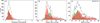 |
Fig. B.4. Same as Fig. 10 but for the F2 (μ = 0.79) flare. |
| In the text | |
Current usage metrics show cumulative count of Article Views (full-text article views including HTML views, PDF and ePub downloads, according to the available data) and Abstracts Views on Vision4Press platform.
Data correspond to usage on the plateform after 2015. The current usage metrics is available 48-96 hours after online publication and is updated daily on week days.
Initial download of the metrics may take a while.