| Issue |
A&A
Volume 705, January 2026
|
|
|---|---|---|
| Article Number | A210 | |
| Number of page(s) | 17 | |
| Section | Planets, planetary systems, and small bodies | |
| DOI | https://doi.org/10.1051/0004-6361/202557014 | |
| Published online | 22 January 2026 | |
TOI-333b: A Neptune-desert planet around an F7V star
1
Departamento de Astronomía, Universidad de Chile,
Casilla 36-D,
Santiago,
Chile
2
Centro de Astrofísica y Tecnologías Afines (CATA),
Casilla 36-D,
Santiago,
Chile
3
Instituto de Estudios Astrofísicos, Universidad Diego Portales,
Av. Ejército 441,
Santiago,
Chile
4
Instituto de Astronomía, Universidad Católica del Norte,
Angamos 0610,
Antofagasta
1270709,
Chile
5
Department of Physics “Ettore Pancini”, University of Naples Federico II,
Naples,
Italy
6
Department of Physics and Astronomy, Vanderbilt University,
Nashville,
TN
37235,
USA
7
Astrobiology Research Unit, Université de Liège,
Allée du 6 août 19,
Liège
4000,
Belgium
8
Astronomy Unit, Queen Mary University of London,
Mile End Road,
London
E1 4NS,
UK
9
Department of Physics, University of Warwick,
Gibbet Hill Road,
Coventry
CV4 7AL,
UK
10
Centre for Exoplanets and Habitability, University of Warwick,
Gibbet Hill Road,
Coventry
CV4 7AL,
UK
11
Center for Astrophysics | Harvard & Smithsonian,
60 Garden Street,
Cambridge
MA
02138,
USA
12
Kotizarovci Observatory,
Sarsoni 90,
51216
Viskovo,
Croatia
13
Observatoire astronomique de l’Université de Genève,
Chemin Pegasi 51,
1290
Versoix,
Switzerland
14
SETI Institute, Mountain View, CA 94043 USA/NASA Ames Research Center,
Moffett Field,
CA
94035,
USA
15
Noqsi Aerospace Ltd.,
15 Blanchard Avenue,
Billerica,
MA
01821,
USA
16
NASA Goddard Space Flight Center,
8800 Greenbelt Rd,
Greenbelt,
MD
20771,
USA
17
Department of Physics and Astronomy, University of New Mexico,
210 Yale Blvd NE,
Albuquerque,
NM
87106,
USA
18
School of Physics and Astronomy, University of Leicester,
Leicester
LE1 7RH,
UK
★ Corresponding author: This email address is being protected from spambots. You need JavaScript enabled to view it.
; This email address is being protected from spambots. You need JavaScript enabled to view it.
Received:
28
August
2025
Accepted:
12
November
2025
Abstract
Observations have shown that planets similar to Neptune are rarely found orbiting Sun-like stars with periods up to ∼4 days. This defines the so-called Neptune desert region. The detection of each individual planet in this region therefore holds a high value by providing detailed insights into the formation and evolution of this population. We report the detection of TOI-333b, a Neptune-desert planet with a mass, radius, and bulk density of 20.1 ± 2.4 M⊕, 4.26 ± 0.11 R⊕, and 1.42 ± 0.21 g cm−3. The planet orbits an F7V star every 3.78 d, whose mass, radius, and effective temperature are of 1.2 ± 0.1 M⊙, 1.10 ± 0.03 R⊙, and 6241−62+73 K, respectively. TOI-333bis likely younger than 1 Gyr, which is supported by the doublet Li line around 6707.856 Å and its comparison to Li abundances in open clusters with well-constrained ages. The planet is expected to host only a 8.5−8.3+10.9% gas-to-core mass ratio for an H/He envelope. On the other hand, models of irradiated ocean worlds predict a 20−10+11% H2O mass fraction with a core fraction of 35−23+20%. We therefore expect that the internal composition of TOI-333bis dominated by a pure rocky composition with almost no H/He envelope, or a rocky world with almost equal mass fraction of water. Finally, TOI-333bis more massive and larger than 77% and 82% of its Neptune-desert counterparts, and its host ranks among the hottest known stars for Neptune-desert planets. This makes this system a unique laboratory for studying the evolution of these planets around hot stars.
Key words: techniques: photometric / techniques: radial velocities / planets and satellites: detection / planets and satellites: fundamental parameters / planets and satellites: general / stars: general
© The Authors 2026
 Open Access article, published by EDP Sciences, under the terms of the Creative Commons Attribution License (https://creativecommons.org/licenses/by/4.0), which permits unrestricted use, distribution, and reproduction in any medium, provided the original work is properly cited.
This article is published in open access under the Subscribe to Open model. This email address is being protected from spambots. You need JavaScript enabled to view it. to support open access publication.
1 Introduction
Shortly after the launch of the Kepler Space Telescope (Borucki et al. 2010), the detection of thousands of exoplanets and planet candidates transformed our understanding of the planetary population in the Galaxy. It quickly became evident that the most common types of planets are super-Earths and sub-Neptunes, which orbit approximately 30% of Sun-like stars (Fressin et al. 2013; Mulders et al. 2018). The Kepler mission also revealed the existence of the so-called Neptune desert (ND), an area in the period-radius-mass parameter space that shows a significant dearth of planetary systems (Szabó & Kiss 2011; Mazeh et al. 2016; Castro-González et al. 2024). The region extends to orbital periods of ~4 days, planetary radii between roughly 2 and 10 R⊕, and masses of about 0.03-0.1 MJ. Additionally, the ND is further corroborated by the scarce number of detections from subsequent space- (e.g., TESS; Ricker et al. 2015) and ground-based missions (e.g., NGTS; Wheatley et al. 2018), but a few outstanding discoveries have been made. For example, LTT9779b (Jenkins et al. 2020), an ultra-hot planet for which recent studies (Hoyer et al. 2023; Reyes et al. 2025; Saha et al. 2025) indicated a likely metal-rich atmosphere and silicate clouds, TOI-824 (Burt et al. 2020), a nearby planet that is twice as dense as Neptune, and TOI-849b (Armstrong et al. 2020), an exposed core of what might have been a giant planet.
The ND population has steadily been growing, and each new detection proved particularly valuable. This is especially true for transiting planets, whose key parameters (e.g. radii, densities, and secondary eclipses) can be measured. The study of transiting ND planets thus enables robust statistical analyses aimed at investigating the likely origins of the ND and understanding its subsequent evolution. For instance, it has been shown that the envelope mass fractions of short-period NDs approach zero, and their host stars are also more metal rich (Des Etangs 2007; Doyle et al. 2025; Vissapragada & Behmard 2025). This might indicate that close-in NDs are the remnants of gas giants, which in turn indicates that distinct evolutionary pathways might act as a function of the orbital period, but also of the host metallic-ity. Moreover, the planet radius and mass distributions for ND planets steeply rise toward smaller, lower-mass planets, following well-established power-law trends Lopez & Jenkins (2012); Petigura et al. (2013). Consequently, larger Neptunes with radii between 4 and 6 R⊕ are relatively rare. They orbit only ~3% of the stars. Additionally, long ultra-short period (USP) Neptunes (R ~ 2-6 R⊕) belong to the rarest detected planets, and Kepler found virtually none.
Neptune-desert planets are expected to retain substantial atmospheres overlying rocky or icy cores. This makes them crucial benchmarks for studying the physics and chemistry of planets in the non-gas giant regime. In particular, the atmospheres of USP and ultra-hot Neptunes exceed 2000 K, and intense irradiation drives a rich mix of neutral and ionised species along with exotic cloud formations (Crossfield et al. 2020; Dragomir et al. 2020). These extreme environments offer unique laboratories for probing atmospheric chemistry under conditions that cannot be reproduced elsewhere. Additionally, the upper atmospheres of these planets can reach escape velocity, which leads to strong atmospheric outflows. As a result, they serve as prime targets for investigating atmospheric mass-loss processes (e.g., Mansfield et al. 2018).
Although the exact origin of the ND is still unknown, our current leading description involves a combination of tidal migration and photoevaporation (Lopez & Fortney 2013; Owen & Wu 2017). Recent theoretical and observational studies have argued that photoevaporation alone may not be strong enough to shape the upper desert boundary. Instead, tidal migration and tidal disruption appear to be more plausible mechanisms (Owen & Lai 2018; Vissapragada et al. 2022). Additionally, Roche-lobe overflow (RLO) is likely to play a significant role in stripping massive envelopes from planets that are extremely close to their host stars on orbital periods of two days or shorter (Valsecchi et al. 2015; Jackson et al. 2016). Therefore, the detection of ND planets and their subsequent follow-up are key to providing insights into the physical processes that create and maintain this region.
We report the discovery of TOI-333b, a short-period planet located in the ND, with a mass of 20.1 ± 2.4 M⊕, radius of 4.26 ± 0.11 R⊕, and bulk density of 1.42 ± 0.21 g cm−3. The planet orbits an F7V-type star every 3.78 days. The host star mass is 1.2 ± 0.1 M⊙, the radius is 1.10 ± 0.03 R⊙, and the effective temperature is  K. In Section 2 we describe the multi-instrument observations that led to the detection of the planet. Section 3 outlines the photometric validation process, along with the derivation of stellar properties and planetary parameters. Sections 4 and 5 present the discussion and conclusions, respectively.
2 Observations
We describe the photometric and spectroscopic time-series acquisition and data reductions that led to the discovery of TOI-333b. Tables A.1 and A.2 show a portion of the photometry and radial velocity (RV) for guidance. The complete dataset is made available through the online supplementary material.
2.1 TESS photometry
TOI-333 was first observed by the Transiting Exoplanet Survey Satellite (TESS; Ricker et al. 2015) in Sectors 02, 29, and 69 with cadences of 30, 2, and 2 minutes, respectively. The data were acquired from the Mikulski Archive for Space Telescopes (MAST), using the lightkurve package (Lightkurve Collaboration 2018). The image data were reduced and analysed by the Science Processing Operations Center at NASA Ames Research Center. We opted to use the PDC_SAP (Smith et al. 2012; Stumpe et al. 2012, 2014) photometric time series from the Science Processing Operations Center (SPOC; Jenkins et al. 2016; Caldwell et al. 2020), which are reduced and analysed at NASA Ames Research Center, because their overall scatter is lower than that of other pipelines. Nonetheless, we inspected the data from the Quick Look Pipeline (QLP; Kunimoto et al. 2021), which confirmed the transit events there as well.
The transit signal was initially identified in ful-frame image (FFI) data by the QLP at MIT (Huang et al. 2020a,b). The TESS Science Office (TSO) subsequently reviewed the vetting products and issued an alert on 20 December 2018 (Guerrero et al. 2021). We then performed an independent transit search using the transit least-squares (TLS) algorithm (Hippke & Heller 2019), and wedetected a total of 18 events. A prominent signal was found at a period of 3.785 days, which prompted a validation process to determine whether the signal originated from a transiting hot Neptune or was instead a false positive.
As part of our photometric vetting, we examined the transit morphology for signs of odd-even depth differences or V-shaped profiles indicative of background eclipsing binaries. Additionally, we note that the SPOC pipeline provides centroid diagnostics that assess the location of the transit signal relative to the nominal TIC host (Twicken et al. 2018). For this candidate, the offset was measured to be 1.1 ±2.8 arcseconds, which is consistent with the signal originating from TIC 224245334, as shown in Fig. 4.
Fig. 1 (left) shows the detrended phase-folded light curves well as the best-fitting transit model derived in Sect. 3.3.
2.2 LCOGT ground-based photometry
We observed a TOI-333 full-transit window on UTC 2021 September 10 in Sloan i′ band from the Las Cumbres Observatory Global Telescope (LCOGT) (Brown et al. 2013) 1.0 m network node at the South Africa Astronomical Observatory near Sutherland, South Africa (SAAO). The 1 m telescope is equipped with a 4096 × 4096 SINISTRO camera with an image scale of 0″.389 per pixel, resulting in a 26′ × 26′ field of view. The images were calibrated by the standard LCOGT BANZAI pipeline (McCully et al. 2018), and differential photometric data were extracted using AstroImageJ (Collins et al. 2017). We used a circular 7″.8 photometric target star aperture that excluded all flux from the nearest known star (Gaia DR3 6535750174975363712), which is 22" north of TOI-333. We detected the transit in the target star photometric aperture, which confirmed that the TESS-detected event indeed occurred in TOI-333.
Fig. 1 (centre) shows the phase-folded LCOGT follow-up photometry from 2021 September 10 with the best-fitting transit model found from the global modelling in Sect. 3.3. We also observed TOI-333in six prior epochs (from August 2019 through August 2021), but a transit event was ruled out. After the ephemeris was revised based on the TESS sector 69 data, the six earlier observation windows were determined to be out of transit.
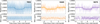 |
Fig. 1 Left : TESS-detrended light curve phase-folded to the best-fitting period listed in Table 2 and zoomed to show the transit event. The blue and white circles correspond to modelled photometric data and binned data with the associated photon noise error. The blue line and shaded region show the median transit model and its 1σ confidence interval. Centre : same as the left panel for the LCOGT-SAAO telescope. Right : same as the left panel for the NGTS mission. Bottom : Residuals of the best-fit model. |
2.3 NGTS photometry
The Next Generation Transit Survey (NGTS; Wheatley et al. 2018) consists of 12 telescopes operating at the ESO Paranal Observatory in Chile and is designed to detect new transiting planetary systems. Each telescope has an aperture of 0.2 m and an individual field of view of 8 deg2, resulting in a combined wide-field coverage of 96 deg2. The detectors feature a 2K × 2K pixel array with 13.5 μm pixels, corresponding to an on-sky resolution of 4.97 arcsec. These high-sensitivity detectors operate over a wavelength range of 520-890 nm. The setup enables 150 ppm photometric precision for bright stars (V < 10 mag) in multi-camera mode, while single-telescope observations at a 30-minute cadence achieve a precision of 400 ppm (Bayliss et al. 2022). The mission has detected 28 planets thus far, from giant hot Jupiters such as NGTS-6 (Vines et al. 2019) and NGTS-21 (Alves et al. 2022) to sub-Neptune-sized planet such as NGTS-4 (West et al. 2019). The NGTS treasure trove also includes the discovery of a remarkably young HJ with an age of ~30 Myr (NGTS-33b; Alves et al. 2025).
TOI-333 follow-up with NGTS occurred during 2024 on September 1, September 19, and October 27, where eight, six, and six telescopes were employed, respectively. A continuum and two transits were captured and a total of 728 images acquired, with an exposure time of 10 seconds per frame. Aperture photometry was extracted with the package CASUTools1, and nightly trends such as atmospheric extinction were corrected for with an adapted version of the SysRem algorithm (Tamuz et al. 2005).
Fig. 1 (right) shows the NGTS detection light curve wrapped around the best-fitting period 3.785257 ± 0.000003 d computed from the global modelling (Sect. 3.3). For a detailed description of the NGTS mission, data reduction, and acquisition, we refer to Wheatley et al. (2018).
2.4 HARPS spectroscopy
TOI-333has been part of our programme to detect and characterise ND planets, where 37 high-resolution Echelle spectra were obtained during UT 2022 July 02 through 2024 August 14 under the programme IDs 109.2374 and 113.26GX (PI: Jenkins) and 112.25QD (PI: Alves), with the HARPS spectrograph on the ESO 3.6 m (Mayor et al. 2003) telescope at the La Silla Observatory in Chile. A total of 21.42 hours were dedicated to TOI-333with exposure times of 1800-2100 seconds, depending on weather and seeing conditions. The high-accuracy mode (HAM) was used and achieved a typical S/N ratio of 25 per pixel at 6500 Å and an RV precision of ~8 m s−1. The standard HARPS pipeline (Lovis & Pepe 2007) was used to compute the RVs, where we opted for a G2 binary mask because it is best suited for TOI-333, which is a late F-type star. Fig. 3 presents the HARPS-modelled RVs in light brown, and the periodogram of the RV residuals is shown in Fig. A.4 in the appendix. No statistically significant signal is found above the 10% false-alarm probability (FAP).
We performed a spectral line diagnostics analysis to assess whether stellar activity might affect the RV signals. Specifically, we searched for periodicities in the generalised Lomb-Scargle periodograms of the bisector velocity span (BIS), the full width at half maximum (FWHM), and the contrast of the crosscorrelation function (CCF), all derived using the HARPS DRS pipeline. No significant signal, particularly close to the planet period, was found, however, as shown in Fig. 2. Finally, we computed the Pearson r coefficient to investigate the correlation between the RVs, against BIS, FWHM-CCF and contrast as correlations would indicate instrumental and/or stellar effects might affect the observed spectral lines. We found weak correlations as a function of BIS, FWHM-CCF, and contrast, with values of 0.07, 0.21, and −0.4, respectively.
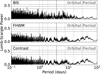 |
Fig. 2 Periodogram of the line bisectors (top panel), CCF-FWHM (centre panel), and contrast (bottom panel) for HARPS (in black). The orbital period of the planet is highlighted by the vertical grey line, and the dashed lines show the harmonics at 1/8, 1/4, 1/2, 2, and 3 from left to right. The top to bottom dashed black lines represent the FAP at 0.1% 1%, and 10%. |
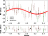 |
Fig. 3 Top : radial velocity phase-folded to the best-fitting period listed in Table 2. The RV data are colour-coded in brown and green for HARPS and FEROS, respectively, and the black circles represent the binned RVs. The red curve and shaded light red region shows the Keplerian model and its 1σ confidence interval. Bottom : residuals of the best-fit model. |
2.5 FEROS spectroscopy
We obtained seven high-resolution echelle spectra using the FEROS spectrograph on the MPG/ESO 2.2 m (Kaufer et al. 1999) telescope at the La Silla Observatory in Chile. The observations ran from UT 2023-09-16 through 2023-09-28 under the programme ID 0111.A-9019(A) (PI: Moyano), with exposure times of 1200-1800 seconds, depending on weather conditions. The automated CERES pipeline (Brahm et al. 2017) was used for the data reduction, and all steps from optimum spectral extraction, wavelength calibration, correction for instrumental drift, and continuum normalisation were performed. Finally, CERES calculated the RVs using the CCF method with a G2 mask, leading to a typical SNR of 21 and an RV precision of 14 m s−1.
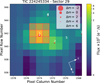 |
Fig. 4 TESS sector 29 full-frame image cutout (11 × 11 pixels) generated with the tpfplotter script described by Aller et al. (2020). TOI-333bis shown in the centre, labeled 1, followed by GAIA DR3 6535747602288702720 (2), at G = 14.11 mag, and 51" away from the planet. The star did not contribute significant flux to the aperture, and only negligible dilution was therefore observed in TESS. |
2.6 Speckle imaging
Stellar companions or background eclipsing binaries might cause periodic dips in the photometric time series. To rule these events out and further ensure that the origin of the transit signal occurred on TOI-333, we performed high angular resolution imaging with the 4.1 m Southern Astrophysical Research (SOAR) telescope (Tokovinin 2018) at Cerro Pachón NoirLab facility and the Very Large Telescope (VLT) at the ESO Paranal Observatory, Chile. SOAR observed TOI-333 on May 18, 2019, with the HRCam camera using the I filter (879 nm), as shown in Fig. A.2. Additionally, a high-resolution image was obtained with the NaCO instrument on the Very Large Telescope (VLT) with adaptive optics (AO) using the Ks (2.2 μm) filter on June 29, 2019. This is shown in Fig. A.3. The differential contrast was estimated to be ~5.4 mag and ~5 mag at 1 arcsec for HRCam/SOAR and NaCO/VLT-UT4, respectively. This provides evidence that TOI-333 is likely single. The high-resolution speckle imaging combined with transits from the TESS, LCOGT-SAAO, and NGTS missions and RVs from HARPS and FEROS makes us confident that the TOI-333bsignal has a planetary origin.
3 Data analysis
3.1 Photometric vetting with DAVE
We employed the pipeline called discovery and vetting of exoplanets (DAVE; Kostov et al. 2019) to analyse transit events in two layers of scrutiny: by examining the image pixels, and by studying the light curve. The centroid module generates an image by subtracting the image taken during the transit from the one taken outside the transit. It then fits a model to this difference image to determine from where the light comes. This helps us to verify whether the dip in brightness really originates from the target star or from a nearby star. If the photocenter shifts away from the target star position, the signal might be a false positive (FP). A clear offset was only detected when the shift remained within the aperture mask we used to retrieve the transit, however. The Modelshift module creates a phase-folded light curve using a trapezoid-shaped model of the transit. Its main goal is to determine whether the signal might come from an eclipsing binary. This allowed us to inspect features such as the transit shape or whether odd and even dips were different, which would indicate a binary system. DAVE also generates some additional diagnostics to help when the target is particularly tricky. The Lomb-Scargle periodogram searches for repeating patterns in the light curve, which might come from the stellar rotation or from nearby stars. These effects can be caused by ellipsoidal variation in binary systems, for instance (Morris & Naftilan 1993; Faigler & Mazeh 2011; Shporer 2017). When strong variations are present, we first removed them (detrended the light curve) for a cleaner analysis.
We vetted the transit events of TOI 333b that occurred in the TESS sectors 02, 29, and 69 by using DAVE. It passed all the tests as a bona fide planet candidate. We report the Modelshift and the centroids modules for TOI 333b obtained for TESS sector 02 in Figs. 5 and 6. The Modelshift returned a clear primary transit well above the noise level, without any statistical significant difference between odd and even transits. Moreover, there is no evidence of a secondary feature that might have been caused by the occultation if TOI-333bwere an eclipsing binary. Based on the centroids module, the overall photocenter is consistent with the position of the target, despite a negligible offset caused by contamination of nearby resolved sources. The brightest pixel in the difference image perfectly corresponds to the target position, however. The Lomb-Scargle Periodogram did not highlight any modulation of the light curve that would be compatible with ellipsoidal variations typical of a binary star system.
Finally, we note that TESS has a large pixel size, about 21" per pixel, and a slightly blurred focus, which means that light from nearby or background stars can be mixed into the same pixel. This can cause problems even when the centroid module is not shifted in the image. Other stars within a single pixel can still affect the transit signal. In some cases, this additional light can cause the transit to look shallower than it really is, which leads to an underestimated planet size. In worse cases, the transit might not come from the target star at all. To avoid these issues, we searched star catalogues (Wenger et al. 2000; Gaia Collaboration 2021) for any nearby stars within the aperture we used to extract the light curve. We found no unresolved stars that might contaminate the light from TOI 333. This confirmed that the transit signal is clean.
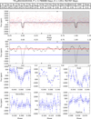 |
Fig. 5 Modelshift module of TOI 333b obtained in TESS sector 02. The first panel displays the phase-folded light curve with the best-fit trapezoid transit model (black line). The second panel shows the convolved light curve with the transit model and noise level (blue lines). The lower panels offer close-ups of the primary and secondary events, both odd and even primaries, and any additional events. The upper panel indicates the statistical significance of these features and highlights them in red when they are flagged as significant by the pipeline. |
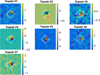 |
Fig. 6 centroids module for the planet candidate TOI 333b for the seven transits detected in TESS sector 02. The dashed white lines outline the aperture mask for light-curve extraction. The star symbol indicates the catalogued position of the target, and individual photocenters are marked by small red dots. The colour bar indicates the number of electrons/s for each case. A centroid image is reliable when no artefacts occur within the aperture mask, e.g. for transits 1, 3, 5, and 6. |
3.2 Stellar properties
The stellar parameters and chemical abundances for TOI-333 were computed with the spectroscopic parameters and atmospheric chemistry of stars (SPECIES2; Soto & Jenkins 2018) and the spectral energy distribution Bayesian model averaging fitter (ARIADNE3; Vines & Jenkins 2022) from spectroscopic analysis and archival photometry spectral energy distribution (SED) fitting. Finally, we independently derived the stellar parameters with PHOENIX stellar atmosphere models and EXOFASTV2.
3.2.1 SPECIES+ARIADNE
Atmospheric parameters such as effective temperature (Teff), metallicity [Fe/H], surface gravity (log g), and micro-turbulence velocity (ξt) were estimated from HARPS high-resolution spectra using the equivalent width (EW) method implemented in SPECIES. The coadded spectra were handed to SPECIES, which computed the EW for the Fe I and Fe II lines. Astrometric and photometric archival data were fetched from databases like Vizier4 and used to compute the initial guesses for the atmospheric parameters. The starting values, EW, and a grid of atmospheric models from ATLAS9 (Castelli & Kurucz 2003) were introduced into MOOG (Sneden 1973), which solved the radiative transfer equation (RTE) while measuring the correlation between Fe line abundances as a function of excitation potential and EW, assuming local thermodynamic equilibrium (LTE). During the search for the RTE solution, an iterative process was carried out up to 10000 times or until atmospheric parameters that lead to no correlation between the iron abundances and the excitation potential and the reduced equivalent width (EW∕λ) were found. The adopted Teff, [Fe/H], and log g along with the parallax, photometry in several bands, and proper motions were used to compute the mass, radius, and age from the isochrone package (Morton 2015) by interpolating through a grid of MIST (Dotter 2016) evolutionary tracks. Nested sampling (Feroz et al. 2009) was used to properly estimate the posterior distributions for Ms,Rs, and age. Finally, SPECIES estimated stellar rotation (v sin i) and macro-turbulent velocities from temperature calibrators and fitted the absorption lines of observed spectra with synthetic line profiles. From our analysis using SPECIES, we derived the following stellar properties for TOI-333 with median and 1σ confidence intervals: Teff = 6267 ± 50 K, [Fe/H] = 0.00 ± 0.05 dex, log g = 4.42 ± 0.08, and v sin i = 6.18 ± 0.70 km/s. The chemical abundances are given in Table A.5.
We used the publicly available Python tool ARIADNE (Vines & Jenkins 2022) to derive the parameters for TOI-333. The code is based on the SED-fitting method, which consists of fitting archival photometry to synthetic magnitudes from interpolated grids of stellar atmosphere models. The synthetic photometry was computed by convolving a given model with several filter-response functions (see available SED models in Vines & Jenkins 2022) and scaled by (R∕D)2. An excess noise term was introduced for each photometric measurement in order to account for underestimated uncertainties. Finally, a cost function with input parameters Teff, log g, [Fe/H], and V-band extinction (Av) was explored with (DYNESTY Speagle 2020), which is a nested sampling algorithm that we used to effectively search the global minimum of the parameter space. We thus determined the best set of synthetic fluxes from a given SED model with stellar properties that best match the observed photometry.
ARIADNE performed the steps laid out above for several atmosphere libraries, from which we used Phoenix V2 (Husser et al. 2013), BT-Settl (Hauschildt et al. 1999; Allard et al. 2012), Castelli & Kurucz (2003), and Kurucz KURUCZ (1993) models. The estimated stellar posterior distributions from each library were weighted by their Bayesian evidence and were averaged to build the adopted final stellar parameter distributions. The Bayesian averaging method helped us to mitigate biases and uncertainties from the assumptions and limitations of individual stellar atmosphere models. This yielded precise stellar parameters, in particular, the Rs and Teff, which were key to inform the global modelling of TOI-333b(see Sect. 3.3). Finally, Teff, log g, [Fe/H], and additional quantities such as D, Rs, and Av from ARIADNE were used to derive the stellar age (ts), Ms, and the equal evolutionary points from the isochrone package.
We started ARIADNE with the priors defined in Table A.4, centred on the SPECIES posterior distributions, but with slightly broader variances to allow a more extensive exploration of the parameter space. N(μ,σ2) represents a Gaussian prior with μ and σ as mean and variance, respectively. The best-fitting ARIADNE SED model is shown in Fig. 7, with the adopted stellar parameters median and 1-σ in Table 1 along with the archival photometry. The SED shows two observed magnitudes (cyan) that deviate from the expected model (black) and the synthetic magnitudes (purple) around 0.8-0.9 μm. We reran ARIADNE without these photometric bands and confirmed that their removal did not yield statistically significant changes in the derived stellar parameters. Therefore, we retained all available photometric data.
We compared our results with the stellar parameters of GAIA DR35 (Vallenari et al. 2023), which agree with our adopted values from ARIADNE. The GAIA parameters are as follows: Teff =  K, log g = 4.341±0.004 dex, Rs = 1.15±0.01 R⊕, ts = 4.9 ± 0.8 Gyr, a distance of 347±2pc, and Av =
  . Finally, we adopted the ARIADNE stellar parameters for TOI-333 because its Bayesian framework that combines multiple atmospheric model grids with nested sampling is robust. We then efficiently explored the parameter space and mitigated limitations inherent to individual atmospheric libraries. The derived results are consistent with the independent analysis presented in Sect. 3.2.2.
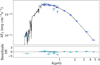 |
Fig. 7 Top : best-fitting spectral energy distribution (black line) based on Castelli & Kurucz (2003) given the TOI-333 photometric data (cyan points) and their respective bandwidths shown as horizontal error bars. The purple diamonds represent the synthetic magnitudes centred at the wavelengths of the photometric data from Table 1. Bottom : residuals of the best fit in σ. |
3.2.2 Independent stellar parameter analysis
Stellar parameters with PHOENIX models
We performed an analysis of the broadband SED of the star together with the Gaia DR3 parallax (with no systematic offset applied; see, e.g., Stassun & Torres 2021) in order to determine an empirical measurement of the stellar radius, following the procedures described by Stassun & Torres (2016); Stassun et al. (2017, 2018). We pulled the JHKS magnitudes from 2MASS, the GGBP GRP magnitudes from Gaia, the BTVT magnitudes from Tycho-2, and the W1-W3 magnitudes from WISE. We also used the near ultraviolet magnitude from GALEX and the absolute flux-calibrated spectrophotometry from Gaia. Together, the available photometry spans the full stellar SED over the wavelength range 0.4-20 μm (see Figure A.5).
We performed a fit using PHOENIX stellar atmosphere models (Husser et al. 2013), with the Teff, log g, and metallicity ([Fe∕H]) adopted from the spectroscopic analysis. The extinction, AV, was limited to the maximum line-of-sight value from the Galactic dust maps of Schlegel et al. (1998). The resulting fit (Figure 7) has a reduced χ2 of 1.9, with a best-fit AV = 0.04 ± 0.02. Integration of the (unreddened) model SED gives the bolometric flux at Earth, Fbol = 4.290 ± 0.100 × 10⁻¹⁰ erg s−1 cm−2. The Fbol together with the Gaia parallax directly gives the bolometric luminosity, Lbol = 1.69 ± 0.05 L⊙. The stellar radius follows from the Stefan-Boltzmann relation, giving R* = 1.13 ± 0.03 R⊙. In addition, we estimated the stellar mass from the empirical relations of Torres et al. (2010), giving M* = 1.17 ± 0.07 M⊙.
Finally, we estimated the stellar rotational velocity from the spectroscopic v sin i together with R*, giving Prot/sini = 8.5 ± 0.9 days, from which we used empirical gyrochronology relations (Mamajek & Hillenbrand 2008) to estimate an age of 1.0 ± 0.2 Gyr.
Stellar properties of TOI-333.
EX0FASTv2 analysis
As an additional constraint on the stellar parameters, we performed an analysis using the EXOFASTv26 modelling suite (Eastman 2017). This tool simultaneously fits the SED and the MESA isochrones and stellar tracks (MIST) models (Dotter 2016; Choi et al. 2016). The SED was constructed using available broadband photometry. We adopted the parallax from Gaia DR3, corrected for the global offset following Lindegren et al. (2021). An upper limit on the V-band extinction, AV, was imposed using the dust maps of Schlafly & Finkbeiner (2011). Gaussian priors were placed on Teff, log g, and [Fe/H] based on the spectroscopic analysis described in Section 3.2.1. The resulting stellar parameters are Teff = 6205 ± 45 K, R* = 1.09 ± 0.02R⊙, and M* = 1.05 ± 0.05 M⊙.
As an additional check, we repeated the EXOFASTv2 analysis and replaced the MIST stellar models with the PARSEC models (Bressan et al. 2012). We kept all other inputs and priors identical. The resulting stellar parameters from the SED+PARSEC fit are fully consistent with the MIST-based values, with Teff = 6207 ± 44 K, R* = 1.09 ± 0.02 R⊙, and M* = 1.07 ± 0.05 M⊙.
3.2.3 Insights into the age of TOI-333
Stellar ages are one key ingredient for understanding the formation of the ND. The proposed scenarios for their formation and evolution histories frequently include a combination of planet migration, envelope mass loss through photoevaporation, tidal disruption, or RLO. The physical processes take place at distinct timescales. A reliable age estimate along with several other planetary system parameters such as mass, radius, and bulk densities, particularly their ages, therefore provides insights into the formation and evolution of ND planets.
A typical method for deriving stellar ages consists of using grids of pre-computed stellar evolutionary models described by stellar physical properties such as Teff, Ls, and [Fe∕H]that are interpolated to fit a set of observables. These evolutionary models are then rearranged to tracks of fixed ages called isochrones, from which the stellar ages are estimated. The complexity and strong non-linearity of isochrones along with observational uncertainties make it difficult to precisely estimate stellar ages for stars on or near the main sequence, however.
The age of ARIADNE of  Gyr was computed using the isochrone package, which to 1σ indicates a broad age range from 30 Myr to 4.29 Gyr. In order to increase the precision, we assessed the TOI-333age based on other methods such as (1) the rotation-age correlation, also known as gyrochronology, which assumes that stellar ages are correlated with the rotation period to first order, and (2) the lithium abundance-age correlations, while owing to the lithium volatility with temperature, its abundance is quickly depleted in stellar atmospheres within a few hundred million years of a stellar lifetime, depending on its initial mass (e.g., Christensen-Dalsgaard & Aguirre 2018).
For the gyrochronology method, we compared the models by Barnes (2007); Mamajek & Hillenbrand (2008), and Meibom et al. (2009) to the Prot/sin i derived from v sin i and Rs from Table 1 as a function of colour B-V. The models indicate gyro-ages for TOI-333 in the range of 0.7 to 2.2 Gyr, depending on the selected model. This statistically agrees within 1σ with the adopted age from ARIADNE. Moreover, we searched TESS photometry for brightness variation caused by spots that appear on the stellar disc due to the stellar spin. We first masked the median-normalised transits and binned the time-series to 30 minutes. We then employed the Lomb-Scargle (LS; VanderPlas 2018) as well as the Edelson-Krolik auto-correlation function (ACF; VanderPlas et al. 2012) methods independently in order to search for a photometric rotation period for the joint TESS sectors. The LS first and second highest peaks were ~4.98 at a normalised power of ~0.02 and ~9.43 days at ~0.014, but no significant variability was found in the folded photometry at these peaks within ~120 ppm photometric precision and a false-alarm probability at the highest peak of ~6 × 10⁻¹⁶. The periodograms were also examined on a per sector basis, but no significant peaks were detected. Finally, although the light curves did not present oscillatory patterns, mild variability was detected visually (see Fig. A.1 upper panel). This might be caused by high-latitude spots.
We identified lithium in the TOI-333 spectra at 6707.856 Å. We measured the Li line EW from fitting a doubleGaussian model to the Li and the nearby partially blended FeI 6707.4 Å lines. Fig. A.6 shows the normalised coadded HARPS spectrum around the Li λ 6707.856 Åline. We obtained a value of EW =  m Å from the Li-only Gaussian model in red, where the 1σ errors were derived from bootstrapping with 50 000 iterations. The presence of lithium provides an independent means to provide an upper limit on the system age. Finally, in Fig. A.7, we compare the TOI-333 EW measurement to stars of the same spectral type in open clusters, where age estimates are generally more reliable over field stars. The data were sourced from Albarrán et al. (2020), and we adapted them to display a few clusters, but a comparison can also be made with Fig. 10 in their study. While a detailed Li-age analysis is beyond the scope of this work because lithium depletion is affected by factors including stellar rotation and metallicity, Fig. A.7 suggests that the majority of late F-type stars in older clusters (>1 Gyr) typically exhibit greater lithium depletion than TOI-333. This allowed us to place an upper age limit of ~1 Gyr. This estimate is consistent with the results from ARIADNE and agrees with expectations from gyrochronology models. These indicators suggest that TOI-333is likely young, and we thus adopted an upper age limit of ~ 1 Gyr for the planetary system.
3.3 Global modelling
A joint radial velocity and photometric analysis was performed with the Juliet (Espinoza et al. 2019) package, which is a versatile code wrapped around packages like Batman (Kreidberg 2015) for the light-curve modelling and radvel (Fulton et al. 2018) for the RV analysis. The dataset was comprised of 37 HARPS, 7 FEROS RVs, and a total of 32282 photometric data points from TESS, LCOGT-SAAO, and NGTS.
Each instrument has its own precision and operates under different environmental conditions. This leads to variations in the noise encapsulation in each dataset. As a result, proper modelling is essential to optimally derive the planetary properties. To address this, we incorporated Gaussian processes (GP) into the noise model to account for correlated noise in the light curves and modelled each instrument with an approximate Matérn kernel. While a global GP kernel is generally preferred for accurately modelling stellar activities, we opted for a multiinstrument GP approach because TOI-333 exhibits moderately low activity in the photometry and RVs highlighted in Fig. A.1. No GP was applied to the RVs, as shown by the Keplerian component of the global model in the bottom panel. We note that the GLS presented no significant peak outside the planet period, which might be attributed to RV activities.
No dilution term was introduced because the transit depths from different missions agree statistically, as highlighted in the lower panel of Fig. 8 or in Table A.3. We note that the transit durations are also consistent amongst distinct instruments. We therefore conclude that no dilution treatment is necessary. For the limb darkening, we followed the approach outlined by Kipping (2013) and employed a quadratic parametrisation with q1 and q2, where uniform priors U(0,1) were assigned for each instrument.
The radial velocity part of the global model included a Keplerian, a systemic RV term (γRV) and a white-noise term to account for stellar jitter. The eccentricity e and the argument of periapsis EW were fixed to zero based on model comparison metrics such as their evidence factor ln(Z). The model with fixed e and ω was favoured by a log-evidence difference of ∆ ln Z = 6 compared to the model in which e and ω were allowed to vary under uniform priors U(0.0,0.1) and U(0.0,90°). Nonetheless, we note that computing the TOI-333beccentricity based on our dataset is challenging because the planetary signal amplitude of the system and the mean RV precision are low. Therefore, our run with a free eccentricity provides an upper limit of 0.03 at 1σ, which further shows that TOI-333blikely is on a circular orbit. Finally, due to the high dimensionality of the parameter space, we used the dynamic nested-sampling algorithm (Higson et al. 2019) through DYNESTY with 1300 live points to explore the parameter space, and we derived the solution shown in Table 2.
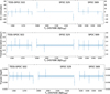 |
Fig. 8 Top : transit-timing variation for the TESS mission. The open blue circles represent each transit time subtracted from the best-fitting linear ephemeris. The pipelines and sectors are labelled at the top. The abscissa was zoomed for better visualisation while avoiding the large gaps in the time domain. Centre : transit-duration variation. The dotted blue and shaded light blue regions represent the transit duration median and its 1σ confidence interval. Bottom : transit depth variation. The colour scheme is the same as above. |
3.4 Transit timing, duration, and depth variation analysis
Transit-timing variations (TTVs; Agol, Steffen, Sari, & Clarkson 2005) arise when observed mid-transit times T0 depart from the predicted values of a linear ephemeris. This is expressed as Tn = T0 + N × P, where N represents the transit number, and P is the orbital period. In other words, the difference between the observed and computed transit times defines the TTV points; a statistically significant deviation from zero would indicate that the planetary orbit has been altered. Two primary causes for TTVs are commonly identified in the literature: (1) dynamical interactions between the planet and its host star, often resulting in angular momentum loss and orbital decay. This might cause the planet to spiral inward towards the star (e.g., WASP-12; Wong et al. 2022). The second cause are (2) gravitational perturbations between planets, particularly near mean-motion resonance (MMR) regions, where the mutual interactions are stronger and produce stronger TTV signals (e.g., WASP-47; Becker et al. 2015). These systems frequently exhibit anti-correlated TTVs and transit-duration variations (TDVs). Notably, numerous multi-planet systems near MMRs detected by Kepler were confirmed through the TTV method alone (Cochran et al. 2011; Gillon et al. 2017; Steffen et al. 2012) because their faint host stars prevented high-precision radial velocity (RV) follow-up. In some cases, RVs have still provided mass estimates (Barros et al. 2014; Almenara et al. 2018), and in others, precise TTV measurements have enabled mass and eccentricity determinations via dynamical modelling (Lithwick et al. 2012). The so-called chopping effect was discovered in this way, which helps us to resolve the mass-eccentricity degeneracy.
TOI-333b TTVs were estimated from the GP-detrended TESS time-series using only transits with a full coverage. Each transit mid-time Tn was modelled with the code batman (Kreidberg 2015), and the final distributions were computed with the affine invariant Markov chain Monte Carlo (MCMC) code implemented in the emcee package (Foreman-Mackey et al. 2013). The transit depth  , normalised semi-major axis
  and a linear offset bl around the normalised flux were free parameters in the model. Tn, p, and a were assigned the following uniform priors: U(Tn−0.05, Tn +0.05), U(p−0.03, p+0.03), U(a−2, a+2), and U(bl−10−4, bl + 10−4), and all other parameters were fixed to their medians from Table 2. Finally, a linear ephemeris model was fit to the Tn, where we used 10 000 MCMC steps, 20% of which were discarded as burn-in. The best-fitting linear model parameters T0 and P for TESS are given by T0 = 2458355.572 ± 0.004 days7 and P = 3.785251 ± 0.000013 days. Using the TESS best-fitting linear ephemerides, we calculated the expected Tn for NGTS and modelled the observed transits Tn. The TTV points for the two NGTS transits are
  min and
  min at 1σ, and the transits are listed in chronological order. NGTS transit durations and depths were fixed to the best-fitting values in Table 2 while computing the individual transits Tn since the relatively short out-of-transit data combined with photometric scatter affected the Tn computation. Likewise, LCOGT-SAAO TTVs are given by
  min at 1σ, while its transit duration and depth are 3.21 ± 0.01 hours and 0.035±0.001. The transit depths, timing, and duration variations are made available in Table A.3. Fig. 8 shows TOI-333bTTV points, that is, the differences between the observed and computed transit times relative to the linear ephemeris model. No significant TTVs were detected. This provides no evidence for changes in the planetary orbit. More data and a longer temporal baseline might help us to further constrain the possible TTV scenarios for this planet.
Planetary properties of TOI-333b.
4 Discussion
In this section, we place TOI-333binto context with the ND population, examine its possible internal structure, and assess its potential for atmospheric characterisation with the James Web Space Telescope (JWST) in Sections 4.1, 4.2 and 4.3, respectively.
4.1 TOI-333b and the Neptune-desert population
Due to its impressively high yield of detected transiting planets, the Kepler Space Telescope (Borucki et al. 2010) has played a major role in mapping out the various populations of worlds in inner planetary systems. From HJs to Earth-like planets, the mission provided a good overview of the Galactic planetary landscape, for example showing that super-Earths and sub-Neptunes orbit ~30% of Sun-like stars (Fressin et al. 2013). In addition, the detection of several ultra-short period (USP; P ≤ 1 day) planets (Sanchis-Ojeda et al. 2013; Rowe et al. 2014), the ND (R*2-10 < R⊕ and P < 4 days), and the regularity of multi-planet systems (e.g., Lissauer et al. 2012; Rowe et al. 2014) were amongst the highlights. Subsequent missions such s TESS (Ricker et al. 2015) not only contributed to confirming the Kepler milestone discoveries, but also expanded the population of all planetary types, including the highly sought-after ND planets (e.g. LTT9779b, TOI-333b, TOI-824b and TOI-849b). This mission also enabled endeavours in planetary and stellar science, such as the study of orbital decay (e.g., WASP-12; Yee et al. 2019), the detection of young planets (e.g., TOI-6442; Alves et al. 2025), and investigations into asteroseismology and gyrochronology in stellar science (Nielsen et al. 2020; Bouma et al. 2023).
The ND region in the mass-period diagram shows a surprising paucity of Neptune-sized planets. The mechanisms proposed to explain this scarcity often involve a combination of planetary migration, atmospheric stripping through photoevaporation, and tidal interactions such as RLO, but the precise evolutionary channels remain uncertain. Thus far, nearly 60 well-studied ND planets have been detected with masses of up to ~31 M⊕. The selected ND sample in this study comes from the TEPCat catalogue of well-studied planets, those with masses up to ~31 M⊕ falling inside the Mazeh et al. (2016) boundaries, highlighted by the green triangular region in Fig. 10. The same figure shows the ND population cumulative distribution highlighting TOI-333bas a green vertical bar, with the width representing the parameter uncertainties. Our analysis revealed a planet that is more massive and larger than 77% and 82%, respectively, of the population, while its orbital distance places it 81.5% farther away, that is, ~18.5 % of the population orbital periods are longer than that of TOI-333b. TOI-333bis hosted by a F7V, which is even more interesting. This is one of the first Neptune-like planets orbiting such a hot star. Only very few ND are detected around stars hotter than G type. This sharp drop-off in their occurrence might be connected to the intense UV/XUV radiation that rapidly strips their atmospheres way. Therefore, TOI-333bcan provide insights into how hot and cool hosts affect the ND planet evolution.
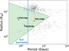 |
Fig. 9 Radius-period diagram for well-studied exoplanets from the TEPCat catalogue (Southworth 2011). TOI-333bis shown as a yellow star within the green triangular region defined by Mazeh et al. (2016), which outlines the ND. The blue and black points represent planets inside and outside this region, respectively, and LTT9779b and TOI-824b are highlighted for comparison. The dashed blue line at P ~ 2 days marks the orbital period below which RLO is thought to significantly affect atmospheric evolution in the desert. |
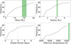 |
Fig. 10 Cumulative distributions for the 60 transiting ND planets, displaying their masses, radii, orbital periods, and effective temperatures of the host star in clockwise order from the top left. The vertical green bars highlight the TOI-333bparameters, where the bar width represents their respective uncertainties. |
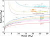 |
Fig. 11 Radius as a function of mass for a set of well-studied ND planets from the TEPCat catalogue. The solid curves show compositional bi-layer models from Zeng et al. 2016, ranging from 100% iron worlds to 100% water planets. The labels are colour-coded to represent the respective model. The dashed line models are taken from (Zeng et al. 2019), showing 2% and 5% H2 envelopes at 1000 K and distinct core compositions. |
4.2 Planet structure and internal composition
Our analysis in Sect. 3.3 revealed a planet slightly larger than Neptune and with a similar mass, with a lower bulk density of 1.42 ± 0.21 g cm−3. In Fig. 11, we compare TOI-333bwith composition models by Zeng et al. (2016, 2019). The planet, represented by the orange star, is most consistent with an H2 envelope surrounding a core composed of H2O, MgSiO3, or more plausibly a mixture of both.
Using smint8 (Structure Model INTerpolator; Piaulet et al. 2021), we investigated the most suitable composition model. The code provides posterior distributions for the planetary core mass fraction (CMF) and the H/He envelope or H2O mass fraction of a planet by interpolating over a set of composition models based on those from Lopez & Fortney (2014); Zeng et al. (2016); Aguichine et al. (2021). smint requires the planetary mass, radius, age, and insolation flux to perform the MCMC samplings. We opted for flat priors based on Tables 1 and 2 and for a chain of 10 000. We discarded 60% in the burn-in step and employed 1000 walkers.
Using Aguichine et al. (2021) irradiated ocean world massradius relations, we found a  H2O mass fraction with a core fraction of
  , representing equal parts of iron and silicate-based chemistry. Additionally, we used smint Lopez & Fortney (2014) models to estimate the gas-to-core mass ratio for a H/He envelope, yielding a fraction of
  . The lack of a significant H/He envelope might indicate that the internal composition of TOI-333bis dominated by a rocky (MgSiO3) composition with almost no H/He envelope or a water-rich world. Nonetheless, we point out that further atmospheric follow-up is necessary to unveil the atmospheric chemistry and provide detailed insights into the planet formation.
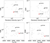 |
Fig. 12 Top : transmission and emission spectroscopy metrics as a function of planetary density for the transiting ND sample, shown as black circles. The black diamonds highlight two benchmark ND planets for comparison with TOI-333b, which is marked by a red star. All TSM and ESM values were computed homogeneously using system parameters from the TEPCat catalogue. Bottom : TSM and ESM plotted against the effective host star temperature. The colour scheme and symbols follow those described in the top panel. |
4.3 Atmospheric follow-up with JWST
The detection of transiting exoplanets has opened the door to studying their atmospheric compositions. Short-period planets continue to be prime targets for an atmospheric characterisation. Planets with high equilibrium temperatures (Teq ≥ 1000 K) and low bulk densities (ρp < 0.3 g cm−3) tend to have extended atmospheres, which allows us to probe material from deeper layers via transmission spectroscopy (Seager & Sasselov 2000). In contrast, secondary eclipse observations make it possible to measure the dayside temperature of the planet and infer its albedo or reflectivity through emission spectroscopy. These techniques have been widely employed using both ground-based facilities (e.g. ESPRESSO/VLT and HIRES/Keck) and space-based observatories such as the HST, Spitzer, and more recently, JWST.
Fig. 12 presents the transmission and emission spectroscopy metrics, called TSM and ESM. They were computed homogeneously using Equations (1) and (4) from Kempton et al. (2018) for the ND population shown in Fig. 9. The benchmark ND planets LTT-9779b and TOI-824b are included for comparison. We note that the TSM value ofTOI-333bis likely within the JWST capabilities, making it a compelling target for atmospheric follow-up. Notably, it lies at the hot end of the Teff-TSM parameter space, where very few ND hosts lie at present (Teff > 6000 K). Therefore, the detection of TOI-333bnot only contributes to the small population of ND planets (currently, ~60 known detections), but also offers a valuable opportunity to probe the atmospheric chemistry of ND planets in the hotter stellar regime, in particular, given that its host star appears to exhibit low activity levels.
5 Conclusions
We reported the discovery of TOI-333b, an ND planet with a mass, radius, and bulk density of 20.1 ± 2.4 M⊕, 4.26 ± 0.11 R⊕, and 1.42 ± 0.21 g cm−3. The planet orbits an F7V star every 3.78 d, whose mass, radius, and effective temperature are 1.2 ± 0.1 M⊙, 1.10 ± 0.03 R⊙, and  K. TOI-333b is likely younger than 1 Gyr and older than a few hundred million years, which is supported the doublet Li line around 6707.856 Å and the comparison to Li abundances in open clusters with well-constrained ages. Its host apparently lacks photometric activity variation, which might indicate a pole-oriented orbit, as was commonly observed for several ND planets, or a relatively quiet star. Finally, TOI-333b is more massive and larger than 77% and 82% of its population, respectively. Furthermore, its host star ranks among the hottest known stars for ND planets, which makes this system a unique laboratory for studying the evolution of these planets around hot stars.
Data availability
The data underlying this article are made available in its online supplementary material as well as through direct emailing the first author. Tables A.1, A.2 and A.3 are available at the CDS via https://cdsarc.cds.unistra.fr/viz-bin/cat/J/A+A/705/A210.
Acknowledgements
DRA acknowledges support of ANID-PFCHA/Doctorado Nacional-21200343, Chile. JSJ greatfully acknowledges support byFONDECYT grant 1201371 and from the ANID BASAL project FB210003. AS postdoctoral fellowship is funded by F.R.S.-FNRS research project ID 40028002 (Detection and Study of Rocky Worlds). EG gratefully acknowledges support from UK Research and Innovation (UKRI) under the UK government’s Horizon Europe funding guarantee [grant number EP/Z000890/1]. ML acknowledges support of the Swiss National Science Foundation under grant number PCEFP2_194576. The contribution of ML has been carried out within the framework of the NCCR PlanetS supported by the Swiss National Science Foundation under grant 51NF40_205606. DJA acknowledges this research was funded in part by the UKRI, (Grants ST/X001121/1, EP/X027562/1). KAC acknowledges support from the TESS mission via subaward s3449 from MIT. We acknowledge the use of public TESS data from pipelines at the TESS Science Office and at the TESS Science Processing Operations Center. Resources supporting this work were provided by the NASA High-End Computing (HEC) Program through the NASA Advanced Supercomputing (NAS) Division at Ames Research Center for the production of the SPOC data products. This work makes use of observations from the LCOGT network. Part of the LCOGT telescope time was granted by NOIRLab through the Mid-Scale Innovations Program (MSIP). MSIP is funded byNSF. This research has also made use of the Exoplanet Follow-up Observation Program (ExoFOP; DOI: 10.26134/ExoFOP5) website, which is operated by the California Institute of Technology, under contract with the National Aeronautics and Space Administration under the Exoplanet Exploration Program. Funding for the TESS mission is provided by NASA’s Science Mission Directorate. The paper is also based on data collected under the NGTS project at the ESO La Silla Paranal Observatory. The NGTS facility is operated by the consortium institutes with support from the UK Science and Technology Facilities Council (STFC) under projects ST/M001962/1, ST/S002642/1 and ST/W003163/1.
References
- Agol, E., Steffen, J., Sari, R., & Clarkson, W. 2005, MNRAS, 359, 567 [Google Scholar]
- Aguichine, A., Mousis, O., Deleuil, M., & Marcq, E. 2021, ApJ, 914, 84 [NASA ADS] [CrossRef] [Google Scholar]
- Albarrán, M. G., Montes, D., Garrido, M. G., et al. 2020, A&A, 643, A71 [NASA ADS] [CrossRef] [EDP Sciences] [Google Scholar]
- Allard, F., Homeier, D., & Freytag, B. 2012, Philos. Trans. Roy. Soc. A: Math. Phys. Eng. Sci., 370, 2765 [Google Scholar]
- Aller, A., Lillo-Box, J., Jones, D., Miranda, L. F., & Forteza, S. B. 2020, A&A, 635, A128 [NASA ADS] [CrossRef] [EDP Sciences] [Google Scholar]
- Almenara, J. M., Diaz, R. F., Hébrard, G., et al. 2018, A&A, 615, A90 [NASA ADS] [CrossRef] [EDP Sciences] [Google Scholar]
- Alves, D. R., Jenkins, J. S., Vines, J. I., et al. 2022, MNRAS, 517, 4447 [Google Scholar]
- Alves, D. R., Jenkins, J. S., Vines, J. I., et al. 2025, MNRAS, 536, 1538 [Google Scholar]
- Armstrong, D. J., Lopez, T. A., Adibekyan, V., et al. 2020, Nature, 583, 39 [Google Scholar]
- Barnes, S. A. 2007, ApJ, 669, 1167 [Google Scholar]
- Barros, S., Díaz, R., Santerne, A., et al. 2014, A&A, 561, L1 [NASA ADS] [CrossRef] [EDP Sciences] [Google Scholar]
- Bayliss, D., O’Brien, S. M., Bryant, E., et al. 2022, in X-Ray, Optical, and Infrared Detectors for Astronomy X, 12191, SPIE, 441 [Google Scholar]
- Becker, J. C., Vanderburg, A., Adams, F. C., Rappaport, S. A., & Schwengeler, H. M. 2015, ApJ, 812, L18 [NASA ADS] [CrossRef] [Google Scholar]
- Borucki, W. J., Koch, D., Basri, G., et al. 2010, Science, 327, 977 [Google Scholar]
- Bouma, L. G., Palumbo, E. K., & Hillenbrand, L. A. 2023, ApJ, 947, L3 [NASA ADS] [CrossRef] [Google Scholar]
- Brahm, R., Jordán, A., & Espinoza, N. 2017, PASP, 129, 034002 [Google Scholar]
- Bressan, A., Marigo, P., Girardi, L., et al. 2012, MNRAS, 427, 127 [NASA ADS] [CrossRef] [Google Scholar]
- Brown, T. M., Baliber, N., Bianco, F. B., et al. 2013, PASP, 125, 1031 [Google Scholar]
- Brown, A. G., Vallenari, A., Prusti, T., et al. 2021, A&A, 649, A1 [NASA ADS] [CrossRef] [EDP Sciences] [Google Scholar]
- Burt, J. A., Nielsen, L. D., Quinn, S. N., et al. 2020, AJ, 160, 153 [Google Scholar]
- Caldwell, D. A., Tenenbaum, P., Twicken, J. D., et al. 2020, RNAAS, 4, 201 [NASA ADS] [Google Scholar]
- Castelli, F., & Kurucz, R. 2003, in IAU Symposium, 210 [Google Scholar]
- Castro-González, A., Bourrier, V., Lillo-Box, J., et al. 2024, A&A, 689, A250 [NASA ADS] [CrossRef] [EDP Sciences] [Google Scholar]
- Choi, J., Dotter, A., Conroy, C., et al. 2016, ApJ, 823, 102 [Google Scholar]
- Christensen-Dalsgaard, J., & Aguirre, V. S. 2018, in Handbook of Exoplanets (Springer), 1679 [Google Scholar]
- Cochran, W. D., Fabrycky, D. C., Torres, G., et al. 2011, ApJS, 197, 7 [NASA ADS] [CrossRef] [Google Scholar]
- Collins, K. A., Kielkopf, J. F., Stassun, K. G., & Hessman, F. V. 2017, AJ, 153, 77 [Google Scholar]
- Crossfield, I. J., Dragomir, D., Cowan, N. B., et al. 2020, ApJ, 903, L7 [NASA ADS] [CrossRef] [Google Scholar]
- Des Etangs, A. L. 2007, A&A, 461, 1185 [NASA ADS] [CrossRef] [EDP Sciences] [Google Scholar]
- Dotter, A. 2016, ApJS, 222, 8 [Google Scholar]
- Doyle, L., Armstrong, D. J., Acuña, L., et al. 2025, MNRAS, 539, 3138 [Google Scholar]
- Dragomir, D., Crossfield, I. J., Benneke, B., et al. 2020, ApJ, 903, L6 [NASA ADS] [CrossRef] [Google Scholar]
- Eastman, J. 2017, Astrophysics Source Code Library, ascl [Google Scholar]
- Espinoza, N., Kossakowski, D., & Brahm, R. 2019, MNRAS, 490, 2262 [Google Scholar]
- Faigler, S., & Mazeh, T. 2011, MNRAS, 415, 3921 [Google Scholar]
- Feroz, F., Hobson, M., & Bridges, M. 2009, MNRAS, 398, 1601 [NASA ADS] [CrossRef] [Google Scholar]
- Foreman-Mackey, D., Hogg, D. W., Lang, D., & Goodman, J. 2013, PASP, 125, 306 [Google Scholar]
- Fressin, F., Torres, G., Charbonneau, D., et al. 2013, ApJ, 766, 81 [NASA ADS] [CrossRef] [Google Scholar]
- Fulton, B. J., Petigura, E. A., Blunt, S., & Sinukoff, E. 2018, PASP, 130, 044504 [Google Scholar]
- Gaia Collaboration (Brown, A. G. A., et al.) 2021, A&A, 649, A1 [NASA ADS] [CrossRef] [EDP Sciences] [Google Scholar]
- Gillon, M., Triaud, A. H., Demory, B.-O., et al. 2017, Nature, 542, 456 [NASA ADS] [CrossRef] [Google Scholar]
- Guerrero, N. M., Seager, S., Huang, C. X., et al. 2021, ApJS, 254, 39 [NASA ADS] [CrossRef] [Google Scholar]
- Hauschildt, P H., Allard, F., & Baron, E. 1999, ApJ, 512, 377 [NASA ADS] [CrossRef] [Google Scholar]
- Henden, A., & Munari, U. 2014, Contrib. Astron. Observ. Skalnate Pleso, 43, 518 [NASA ADS] [Google Scholar]
- Higson, E., Handley, W., Hobson, M., & Lasenby, A. 2019, Statist. Comput., 29, 891 [Google Scholar]
- Hippke, M., & Heller, R. 2019, A&A, 623, A39 [NASA ADS] [CrossRef] [EDP Sciences] [Google Scholar]
- Hoyer, S., Jenkins, J., Parmentier, V., et al. 2023, A&A, 675, A81 [NASA ADS] [CrossRef] [EDP Sciences] [Google Scholar]
- Huang, C. X., Vanderburg, A., Pál, A., et al. 2020a, RNAAS, 4, 204 [Google Scholar]
- Huang, C. X., Vanderburg, A., Pál, A., et al. 2020b, RNAAS, 4, 206 [NASA ADS] [Google Scholar]
- Husser, T-O., Wende-von Berg, S., Dreizler, S., et al. 2013, A&A, 553, A6 [NASA ADS] [CrossRef] [EDP Sciences] [Google Scholar]
- Jackson, B., Jensen, E., Peacock, S., Arras, P., & Penev, K. 2016, Celest. Mech. Dyn. Astron., 126, 227 [NASA ADS] [CrossRef] [Google Scholar]
- Jenkins, J. M., Twicken, J. D., McCauliff, S., et al. 2016, in Software and Cyberinfrastructure for Astronomy IV, 9913, SPIE, 1232 [Google Scholar]
- Jenkins, J. S., Díaz, M. R., Kurtovic, N. T., et al. 2020, Nat. Astron., 4, 1148 [Google Scholar]
- Kaufer, A., Stahl, O., Tubbesing, S., et al. 1999, The Messenger, 95, 8 [Google Scholar]
- Kempton, E. M.-R., Bean, J. L., Louie, D. R., et al. 2018, PASP, 130, 114401 [CrossRef] [Google Scholar]
- Kipping, D. M. 2013, MNRAS, 435, 2152 [Google Scholar]
- Kostov, V. B., Mullally, S. E., Quintana, E. V., et al. 2019, AJ, 157, 124 [NASA ADS] [CrossRef] [Google Scholar]
- Kreidberg, L. 2015, PASP, 127, 1161 [Google Scholar]
- Kunimoto, M., Huang, C., Tey, E., et al. 2021, RNAAS, 5, 234 [NASA ADS] [Google Scholar]
- KURUCZ, R.-L. 1993, Kurucz CD-Rom, 13 [Google Scholar]
- Lightkurve Collaboration (Cardoso, J. V. d. M., et al.) 2018, Lightkurve: Kepler and TESS time series analysis in Python, Astrophysics Source Code Library [Google Scholar]
- Lindegren, L., Bastian, U., Biermann, M., et al. 2021, A&A, 649, A4 [EDP Sciences] [Google Scholar]
- Lissauer, J. J., Marcy, G. W., Rowe, J. F., et al. 2012, ApJ, 750, 112 [NASA ADS] [CrossRef] [Google Scholar]
- Lithwick, Y., Xie, J., & Wu, Y. 2012, ApJ, 761, 122 [Google Scholar]
- Lopez, E. D., & Fortney, J. J. 2013, ApJ, 776, 2 [Google Scholar]
- Lopez, E. D., & Fortney, J. J. 2014, ApJ, 792, 1 [Google Scholar]
- Lopez, S., & Jenkins, J. 2012, ApJ, 756, 177 [Google Scholar]
- Lovis, C., & Pepe, F. 2007, A&A, 468, 1115 [NASA ADS] [CrossRef] [EDP Sciences] [Google Scholar]
- Mamajek, E. E., & Hillenbrand, L. A. 2008, ApJ, 687, 1264 [Google Scholar]
- Mansfield, M., Bean, J. L., Oklopcic, A., et al. 2018, ApJ, 868, L34 [NASA ADS] [CrossRef] [Google Scholar]
- Mayor, M., Pepe, F., Queloz, D., et al. 2003, The Messenger, 114, 20 [NASA ADS] [Google Scholar]
- Mazeh, T., Holczer, T., & Faigler, S. 2016, A&A, 589, A75 [NASA ADS] [CrossRef] [EDP Sciences] [Google Scholar]
- McCully, C., Volgenau, N. H., Harbeck, D.-R., et al. 2018, SPIE Conf. Ser., 10707, 107070K [Google Scholar]
- Meibom, S., Mathieu, R. D., & Stassun, K. G. 2009, ApJ, 695, 679 [Google Scholar]
- Morris, S. L., & Naftilan, S. A. 1993, ApJ, 419, 344 [NASA ADS] [CrossRef] [Google Scholar]
- Morton, T. D. 2015, Astrophysics Source Code Library, ascl [Google Scholar]
- Mulders, G. D., Pascucci, I., Apai, D., & Ciesla, F. J. 2018, AJ, 156, 24 [Google Scholar]
- Nielsen, M. B., Ball, W. H., Standing, M., et al. 2020, A&A, 641, A25 [NASA ADS] [CrossRef] [EDP Sciences] [Google Scholar]
- Owen, J. E., & Lai, D. 2018, MNRAS, 479, 5012 [Google Scholar]
- Owen, J. E., & Wu, Y. 2017, ApJ, 847, 29 [Google Scholar]
- Petigura, E. A., Marcy, G. W., & Howard, A. W. 2013, ApJ, 770, 69 [NASA ADS] [CrossRef] [Google Scholar]
- Piaulet, C., Benneke, B., Rubenzahl, R. A., et al. 2021, AJ, 161, 70 [NASA ADS] [CrossRef] [Google Scholar]
- Reyes, R. R., Jenkins, J. S., Sedaghati, E., et al. 2025, A&A, 695, A26 [NASA ADS] [CrossRef] [EDP Sciences] [Google Scholar]
- Ricker, G. R., Winn, J. N., Vanderspek, R., et al. 2015, J. Astron. Telesc. Instrum. Syst., 1, 014003 [Google Scholar]
- Rowe, J. F., Bryson, S. T., Marcy, G. W., et al. 2014, ApJ, 784, 45 [Google Scholar]
- Saha, S., Jenkins, J. S., Parmentier, V., et al. 2025, A&A, 700, A45 [NASA ADS] [CrossRef] [EDP Sciences] [Google Scholar]
- Sanchis-Ojeda, R., Rappaport, S., Winn, J. N., et al. 2013, ApJ, 774, 54 [Google Scholar]
- Schlafly, E. F., & Finkbeiner, D. P. 2011, ApJ, 737, 103 [Google Scholar]
- Schlegel, D. J., Finkbeiner, D. P., & Davis, M. 1998, ApJ, 500, 525 [Google Scholar]
- Seager, S., & Sasselov, D. D. 2000, ApJ, 537, 916 [Google Scholar]
- Shporer, A. 2017, PASP, 129, 072001 [Google Scholar]
- Skrutskie, M. F., Cutri, R. M., Stiening, R., et al. 2006, AJ, 131, 1163 [NASA ADS] [CrossRef] [Google Scholar]
- Smith, J. C., Stumpe, M. C., Van Cleve, J. E., et al. 2012, PASP, 124, 1000 [Google Scholar]
- Sneden, C. 1973, ApJ, 184, 839 [Google Scholar]
- Soto, M., & Jenkins, J. S. 2018, A&A, 615, A76 [NASA ADS] [CrossRef] [EDP Sciences] [Google Scholar]
- Southworth, J. 2011, MNRAS, 417, 2166 [Google Scholar]
- Speagle, J. S. 2020, MNRAS, 493, 3132 [Google Scholar]
- Stassun, K. G., & Torres, G. 2016, AJ, 152, 180 [Google Scholar]
- Stassun, K. G., & Torres, G. 2021, ApJ, 907, L33 [NASA ADS] [CrossRef] [Google Scholar]
- Stassun, K. G., Collins, K. A., & Gaudi, B. S. 2017, AJ, 153, 136 [Google Scholar]
- Stassun, K. G., Corsaro, E., Pepper, J. A., & Gaudi, B. S. 2018, AJ, 155, 22 [Google Scholar]
- Stassun, K. G., Oelkers, R. J., Pepper, J., et al. 2018, AJ, 156, 102 [Google Scholar]
- Steffen, J. H., Fabrycky, D. C., Ford, E. B., et al. 2012, MNRAS, 421, 2342 [NASA ADS] [CrossRef] [Google Scholar]
- Stumpe, M. C., Smith, J. C., Van Cleve, J. E., et al. 2012, PASP, 124, 985 [Google Scholar]
- Stumpe, M. C., Smith, J. C., Catanzarite, J. H., et al. 2014, PASP, 126, 100 [Google Scholar]
- Szabó, G. M., & Kiss, L. 2011, ApJ, 727, L44 [CrossRef] [Google Scholar]
- Tamuz, O., Mazeh, T., & Zucker, S. 2005, MNRAS, 356, 1466 [Google Scholar]
- Tokovinin, A. 2018, PASP, 130, 035002 [Google Scholar]
- Torres, G., Andersen, J., & Giménez, A. 2010, A&AR, 18, 67 [NASA ADS] [CrossRef] [Google Scholar]
- Twicken, J. D., Catanzarite, J. H., Clarke, B. D., et al. 2018, PASP, 130, 064502 [Google Scholar]
- Vallenari, A., Brown, A., Prusti, T., et al. 2023, A&A, 674, A1 [NASA ADS] [CrossRef] [EDP Sciences] [Google Scholar]
- Valsecchi, F., Rappaport, S., Rasio, F. A., Marchant, P., & Rogers, L. A. 2015, ApJ, 813, 101 [NASA ADS] [CrossRef] [Google Scholar]
- VanderPlas, J., Connolly, A. J., Ivezic, Z., & Gray, A. 2012, in 2012 Conference on Intelligent Data Understanding, IEEE, 47 [Google Scholar]
- VanderPlas, J. T. 2018, ApJSS, 236, 16 [Google Scholar]
- Vines, J. I., & Jenkins, J. S. 2022, MNRAS, 513, 2719 [NASA ADS] [CrossRef] [Google Scholar]
- Vines, J. I., Jenkins, J. S., Acton, J. S., et al. 2019, MNRAS, 489, 4125 [NASA ADS] [CrossRef] [Google Scholar]
- Vissapragada, S., & Behmard, A. 2025, AJ, 169, 117 [Google Scholar]
- Vissapragada, S., Knutson, H. A., dos Santos, L. A., Wang, L., & Dai, F. 2022, ApJ, 927, 96 [NASA ADS] [CrossRef] [Google Scholar]
- Wenger, M., Ochsenbein, F., Egret, D., et al. 2000, A&AS, 143, 9 [NASA ADS] [CrossRef] [EDP Sciences] [Google Scholar]
- West, R. G., Gillen, E., Bayliss, D., et al. 2019, MNRAS, 486, 5094 [Google Scholar]
- Wheatley, P. J., West, R. G., Goad, M. R., et al. 2018, MNRAS, 475, 4476 [Google Scholar]
- Wong, I., Shporer, A., Vissapragada, S., et al. 2022, AJ, 163, 175 [NASA ADS] [CrossRef] [Google Scholar]
- Wright, E. L., Eisenhardt, P. R. M., Mainzer, A. K., et al. 2010, AJ, 140, 1868 [Google Scholar]
- Yee, S. W., Winn, J. N., Knutson, H. A., et al. 2019, ApJ, 888, L5 [Google Scholar]
- Zeng, L., Sasselov, D. D., & Jacobsen, S. B. 2016, ApJ, 819, 127 [Google Scholar]
- Zeng, L., Jacobsen, S. B., Sasselov, D. D., et al. 2019, PNAS, 116, 9723 [Google Scholar]
The unit is in barycentric Julian date in the barycentric dynamical time.
Appendix A Extra tables and figures
Appendix A.1 Photometric and RV time series
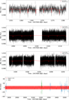 |
Fig. A.1 From top to bottom we show the TESS photometric time series with the best-fitting transit + GP model in red. Cadences are 30, 2, and 2 minutes, respectively. At the bottom, the RV time-series are highlighted with FEROS and HARPS instruments in light green and blue. The best-fitting Keplerian are shown in red. No GPs were used in the RVs part of the global model. |
Appendix A.2 Instrumental photometric time series
TESS, LCOGT-SAAO, and NGTS photometry for TOI-333.
Appendix A.3 Speckle imaging
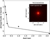 |
Fig. A.2 TOI-333 speckle image obtained with the SOAR telescope showing no nearby binary was observed at 1 arcsec. |
 |
Fig. A.3 TOI-333 speckle image obtained with the NaCo at the VLT telescope indicating that no companions were observed to ∆mag∼5. |
Appendix A.4 RV Residuals Periodogram
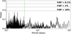 |
Fig. A.4 Lomb-Scargle periodogram on HARPS radial velocity residuals. Dashed black lines show the 0.1%, 1%, and 10% FAP levels (top to bottom). The green vertical bar marks the orbital period of TOI-333b. |
Appendix A.5 PHOENIX SED modelling
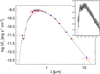 |
Fig. A.5 Spectral energy distribution of TOI-333. Red symbols represent the observed photometric measurements, where the horizontal bars represent the effective width of the passband. Blue symbols are the model fluxes from the best-fit PHOENIX atmosphere model (black). The absolute flux-calibrated Gaia spectrophotometry is shown as the grey swathe; see also the inset plot. |
Appendix A.6 Lithium equivalent width
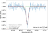 |
Fig. A.6 TOI-3 33 coadded spectra around the Lithium line at 6707.86 Å in blue with a best-fitting double Gaussian model to the Fe (in green) and Li (in red) lines Equivalent width. The total Gaussian model is shown in black. |
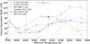 |
Fig. A.7 Open clusters Li EW λ 6707.86A as a function of effective temperature; the data are from (Albarrán et al. 2020) colour coded by cluster age. Circles with the same colour scheme shows the EW median binned for every 100 Teff bins. TOI-333 is represented by the blue star, while the black cross at the top shows the data typical 1σ confidence intervals. |
Appendix A.7 HARPS AND FEROS radial velocities
HARPS and FEROS TOI-333 velocimetry obtained with the HARPS and FEROS spectrographs.
Appendix A.8 Transit timing, duration and depth variations
TOI-333b Transit Timing, Duration and Depth Variations
Appendix A.9 ARIADNE priors for the stellar characterisation
TOI-333 priors used in ARIADNE
Appendix A.10 TOI-333 chemical abundances from SPECIES
TOI-333 chemical abundances from SPECIES
All Tables
HARPS and FEROS TOI-333 velocimetry obtained with the HARPS and FEROS spectrographs.
All Figures
|
Fig. 1 Left : TESS-detrended light curve phase-folded to the best-fitting period listed in Table 2 and zoomed to show the transit event. The blue and white circles correspond to modelled photometric data and binned data with the associated photon noise error. The blue line and shaded region show the median transit model and its 1σ confidence interval. Centre : same as the left panel for the LCOGT-SAAO telescope. Right : same as the left panel for the NGTS mission. Bottom : Residuals of the best-fit model. |
| In the text | |
|
Fig. 2 Periodogram of the line bisectors (top panel), CCF-FWHM (centre panel), and contrast (bottom panel) for HARPS (in black). The orbital period of the planet is highlighted by the vertical grey line, and the dashed lines show the harmonics at 1/8, 1/4, 1/2, 2, and 3 from left to right. The top to bottom dashed black lines represent the FAP at 0.1% 1%, and 10%. |
| In the text | |
|
Fig. 3 Top : radial velocity phase-folded to the best-fitting period listed in Table 2. The RV data are colour-coded in brown and green for HARPS and FEROS, respectively, and the black circles represent the binned RVs. The red curve and shaded light red region shows the Keplerian model and its 1σ confidence interval. Bottom : residuals of the best-fit model. |
| In the text | |
|
Fig. 4 TESS sector 29 full-frame image cutout (11 × 11 pixels) generated with the tpfplotter script described by Aller et al. (2020). TOI-333bis shown in the centre, labeled 1, followed by GAIA DR3 6535747602288702720 (2), at G = 14.11 mag, and 51" away from the planet. The star did not contribute significant flux to the aperture, and only negligible dilution was therefore observed in TESS. |
| In the text | |
|
Fig. 5 Modelshift module of TOI 333b obtained in TESS sector 02. The first panel displays the phase-folded light curve with the best-fit trapezoid transit model (black line). The second panel shows the convolved light curve with the transit model and noise level (blue lines). The lower panels offer close-ups of the primary and secondary events, both odd and even primaries, and any additional events. The upper panel indicates the statistical significance of these features and highlights them in red when they are flagged as significant by the pipeline. |
| In the text | |
|
Fig. 6 centroids module for the planet candidate TOI 333b for the seven transits detected in TESS sector 02. The dashed white lines outline the aperture mask for light-curve extraction. The star symbol indicates the catalogued position of the target, and individual photocenters are marked by small red dots. The colour bar indicates the number of electrons/s for each case. A centroid image is reliable when no artefacts occur within the aperture mask, e.g. for transits 1, 3, 5, and 6. |
| In the text | |
|
Fig. 7 Top : best-fitting spectral energy distribution (black line) based on Castelli & Kurucz (2003) given the TOI-333 photometric data (cyan points) and their respective bandwidths shown as horizontal error bars. The purple diamonds represent the synthetic magnitudes centred at the wavelengths of the photometric data from Table 1. Bottom : residuals of the best fit in σ. |
| In the text | |
|
Fig. 8 Top : transit-timing variation for the TESS mission. The open blue circles represent each transit time subtracted from the best-fitting linear ephemeris. The pipelines and sectors are labelled at the top. The abscissa was zoomed for better visualisation while avoiding the large gaps in the time domain. Centre : transit-duration variation. The dotted blue and shaded light blue regions represent the transit duration median and its 1σ confidence interval. Bottom : transit depth variation. The colour scheme is the same as above. |
| In the text | |
|
Fig. 9 Radius-period diagram for well-studied exoplanets from the TEPCat catalogue (Southworth 2011). TOI-333bis shown as a yellow star within the green triangular region defined by Mazeh et al. (2016), which outlines the ND. The blue and black points represent planets inside and outside this region, respectively, and LTT9779b and TOI-824b are highlighted for comparison. The dashed blue line at P ~ 2 days marks the orbital period below which RLO is thought to significantly affect atmospheric evolution in the desert. |
| In the text | |
|
Fig. 10 Cumulative distributions for the 60 transiting ND planets, displaying their masses, radii, orbital periods, and effective temperatures of the host star in clockwise order from the top left. The vertical green bars highlight the TOI-333bparameters, where the bar width represents their respective uncertainties. |
| In the text | |
|
Fig. 11 Radius as a function of mass for a set of well-studied ND planets from the TEPCat catalogue. The solid curves show compositional bi-layer models from Zeng et al. 2016, ranging from 100% iron worlds to 100% water planets. The labels are colour-coded to represent the respective model. The dashed line models are taken from (Zeng et al. 2019), showing 2% and 5% H2 envelopes at 1000 K and distinct core compositions. |
| In the text | |
|
Fig. 12 Top : transmission and emission spectroscopy metrics as a function of planetary density for the transiting ND sample, shown as black circles. The black diamonds highlight two benchmark ND planets for comparison with TOI-333b, which is marked by a red star. All TSM and ESM values were computed homogeneously using system parameters from the TEPCat catalogue. Bottom : TSM and ESM plotted against the effective host star temperature. The colour scheme and symbols follow those described in the top panel. |
| In the text | |
|
Fig. A.1 From top to bottom we show the TESS photometric time series with the best-fitting transit + GP model in red. Cadences are 30, 2, and 2 minutes, respectively. At the bottom, the RV time-series are highlighted with FEROS and HARPS instruments in light green and blue. The best-fitting Keplerian are shown in red. No GPs were used in the RVs part of the global model. |
| In the text | |
|
Fig. A.2 TOI-333 speckle image obtained with the SOAR telescope showing no nearby binary was observed at 1 arcsec. |
| In the text | |
|
Fig. A.3 TOI-333 speckle image obtained with the NaCo at the VLT telescope indicating that no companions were observed to ∆mag∼5. |
| In the text | |
|
Fig. A.4 Lomb-Scargle periodogram on HARPS radial velocity residuals. Dashed black lines show the 0.1%, 1%, and 10% FAP levels (top to bottom). The green vertical bar marks the orbital period of TOI-333b. |
| In the text | |
|
Fig. A.5 Spectral energy distribution of TOI-333. Red symbols represent the observed photometric measurements, where the horizontal bars represent the effective width of the passband. Blue symbols are the model fluxes from the best-fit PHOENIX atmosphere model (black). The absolute flux-calibrated Gaia spectrophotometry is shown as the grey swathe; see also the inset plot. |
| In the text | |
|
Fig. A.6 TOI-3 33 coadded spectra around the Lithium line at 6707.86 Å in blue with a best-fitting double Gaussian model to the Fe (in green) and Li (in red) lines Equivalent width. The total Gaussian model is shown in black. |
| In the text | |
|
Fig. A.7 Open clusters Li EW λ 6707.86A as a function of effective temperature; the data are from (Albarrán et al. 2020) colour coded by cluster age. Circles with the same colour scheme shows the EW median binned for every 100 Teff bins. TOI-333 is represented by the blue star, while the black cross at the top shows the data typical 1σ confidence intervals. |
| In the text | |
Current usage metrics show cumulative count of Article Views (full-text article views including HTML views, PDF and ePub downloads, according to the available data) and Abstracts Views on Vision4Press platform.
Data correspond to usage on the plateform after 2015. The current usage metrics is available 48-96 hours after online publication and is updated daily on week days.
Initial download of the metrics may take a while.