| Issue |
A&A
Volume 705, January 2026
|
|
|---|---|---|
| Article Number | A110 | |
| Number of page(s) | 10 | |
| Section | Planets, planetary systems, and small bodies | |
| DOI | https://doi.org/10.1051/0004-6361/202557459 | |
| Published online | 12 January 2026 | |
Mapping of the Ganymede surface reflectance from Juno/UVS data
1
Aix-Marseille Université, CNRS, CNES, Institut Origines, LAM,
Marseille,
France
2
Laboratory of Atmospheric and Planetary Physics, STAR Institute, University of Liège,
Belgium
3
Space Science and Engineering Division, Southwest Research Institute,
San Antonio,
TX,
USA
4
University of Bern, Faculty of Science, Physics Institute, Space Research & Planetary Sciences (WP),
Switzerland
5
Department of Physics and Astronomy, The University of Alabama,
Tuscaloosa,
AL
35487,
USA
6
NASA Langley Research Center,
Hampton,
Va,
USA
7
Science Systems and Applications Inc.,
Hampton,
VA,
USA
8
Physique des Interactions Ioniques et Moléculaires, CNRS et Aix-Marseille Université,
France
9
Department of Climate and Space Sciences and Engineering, University of Michigan,
Ann Arbor,
MI,
USA
10
LATMOS/CNRS, Sorbonne Université, UVSQ,
Paris,
France
11
The University of Edinburgh, School of GeoSciences,
Edinburgh,
UK
12
Centre for Exoplanet Science, University of Edinburgh,
Edinburgh,
UK
13
Univ. Grenoble Alpes, CNRS,
IPAG,
38000
Grenoble,
France
14
Univ. Grenoble Alpes,
CSUG,
38000
Grenoble,
France
15
IRAP, CNRS-Université Paul Sabatier,
Toulouse Cedex 4,
France
★ Corresponding author: This email address is being protected from spambots. You need JavaScript enabled to view it.
Received:
28
September
2025
Accepted:
5
December
2025
Abstract
Context. Ganymede is the only moon in the Solar System with an intrinsic magnetic field that actively interacts with the Jupiter magnetosphere. This precipitates energetic electrons that generate ultraviolet (UV) auroral emission.
Aims. In sunlit auroral regions, the observed emission partly overlaps with the solar continuum reflected by the surface. An accurate modeling of the observed UV spectra therefore requires precise knowledge of the surface spectral reflectance.
Methods. We analyzed Juno/UVS data acquired during the 34th perijove (PJ) flyby to constrain the Ganymede surface reflectance in the 140−205 nm range. We used the non-local thermal equilibrium radiative transfer model originally developed to simulate the auroral emission of Ganymede, which also accounts for the reflection of solar flux by the satellite surface, to fit the observed spectra in sunlit auroral regions.
Results. Our results revealed that the reflectance varies strongly spatially and spectrally from 0.1% to 8% in the [140 nm; 205 nm] wavelength range. This indicates a significant surface heterogeneity. This variability likely reflects long-term interactions between the icy surface of Ganymede and precipitating energetic particles, which alter the ice structure and crystallinity and its chemical composition. In addition, the derived reflectance maps show no clear correlation with the visible surface features of Ganymede, suggesting that the UV reflectance is primarily shaped by irradiation-driven processes and not by the geological morphology.
Conclusions. The resulting reflectance maps provide a critical input for future UV auroral emission modeling, particularly in preparation for observations by the Juice/UVS mission.
Key words: plasmas / radiative transfer / planets and satellites: atmospheres / planets and satellites: aurorae / planets and satellites: gaseous planets / planets and satellites: surfaces
© The Authors 2026
 Open Access article, published by EDP Sciences, under the terms of the Creative Commons Attribution License (https://creativecommons.org/licenses/by/4.0), which permits unrestricted use, distribution, and reproduction in any medium, provided the original work is properly cited.
This article is published in open access under the Subscribe to Open model. This email address is being protected from spambots. You need JavaScript enabled to view it. to support open access publication.
1 Introduction
Ganymede hosts bright UV auroral emission generated by electron impact on its tenuous H2, H, H2O, O2, and O (Leblanc et al. 2017; Carnielli et al. 2019; Bockelée-Morvan et al. 2024; Vorburger et al. 2024; Waite et al. 2024) atmosphere. These emissions have been extensively characterized in previous observational and modeling studies, including a detailed analysis of the precipitating electron properties during the Juno 34th perijove (PJ34) flyby (Benmahi et al. 2025). The relative contributions of atmospheric species and electron energies are commonly inferred from the intensity ratio of the 130.4 nm and 135.6 nm oxygen multiplets (e.g. Hall et al. 1998; Molyneux et al. 2018). A full description of the auroral mechanisms of Ganymede and their relation with the energetic particle environment can be found in Benmahi et al. (2025) and is not repeated here.
In sunlit regions, however, the interpretation of these emissions is complicated by the contribution of the solar continuum reflected by the surface. The strength of this reflected component is sensitive to the local UV reflectance, which is spatially variable and wavelength dependent. It is therefore essential to accurately constrain the reflectance for interpreting auroral observations and for modeling the interaction between the Jupiter magnetosphere and the surface of Ganymede.
The close flyby of Ganymede by Juno at an altitude of approximately 1000 km during its 34th perijove (Hansen et al. 2022; Waite et al. 2024) provided a unique opportunity to measure the in situ electron and ion populations near the satellite using the instruments JADE (Jovian Auroral Distributions Experiment) and JEDI (Jupiter Energetic Particle Detector Instrument) (Allegrini et al. 2022). Based on these observations, Vorburger et al. (2024) developed a 3D model of the Ganymede atmosphere. Building on this framework, Benmahi et al. (2025) constrained the fluxes, energies, and distributions of precipitating electrons using a combination of a non-LTE radiative transfer model that reproduced the observed UV auroral emission of Ganymede, and the electron transport model called TransPlanet (Lilensten et al. 1989; Benmahi 2022; Benmahi et al. 2024a,b; Benne et al. 2024).
In the sunlit auroral regions, the intensity ratio  is also affected by the solar 130.4 nm line reflected by the Ganymede surface. This effect is directly controlled by the local reflectance. Hall et al. (1998) estimated that the mean surface albedo at 135 nm is approximately 2.3%, based on the Hubble Space Telescope (HST) Space Telescope Imaging Spectrograph (HST/STIS) measurements. This global value cannot be used in radiative transfer models, however, which require a high spatial resolution. Benmahi et al. (2025) used Juno Ultraviolet Spectrograph (UVS) (Davis et al. 2011; Gladstone et al. 2017) data from PJ34 and showed that in sunlit auroral regions, the reflectance in the 125−140 nm range varies significantly with location, with values from ∼ 0.6% to ∼ 3%. This reflectance is also wavelength dependent (e.g., Molyneux et al. 2020, 2022). To accurately model auroral emission in the presence of solar reflection, it is therefore essential to account for a reflectance that varies both spatially and spectrally.
The spatial variability in the reflectance reflects a physical heterogeneity that is driven by long-term magnetospheric irradiation, as demonstrated in previous studies (Molyneux et al. 2022). The tenuous atmosphere of Ganymede does not act as an effective shield. Energetic particles can penetrate and directly impact the surface, particularly at high latitudes where magnetic field lines converge. This causes a higher precipitation of electrons and ions (Poppe et al. 2018). Moreover, modeling by Waite et al. (2024) suggested that more than 97% of the electron energy flux below 30 keV reaches the surface.
This bombardment alters the physical and chemical properties of the surface ice. While energetic electron and ion irradiation can break ice grains down, it also preferentially removes the smallest grains, which might increase the average grain size over time (Cassidy et al. 2013). In the polar regions of Ganymede, however, where the surface temperatures are particularly low, small ice grains might be continuously trapped and accumulate due to migration from warmer areas, and a locally smaller average grain size might thus be maintained. These fine grains not only enhance UV reflectance through increased scattering, as suggested by laboratory experiments and observational studies (Molyneux et al. 2020; Bockelée-Morvan et al. 2024), but might also facilitate the adsorption of volatiles such as O2 and CO2, especially in regions with an increased surface roughness where shadowing effects reduce the local insolation and promote retention.
Conversely, the radiolytic production of UV-absorbing compounds such as H2O2 can darken the UV spectrum (by reducing the reflectance), which counteracts this effect (Trumbo et al. 2023). The abundance of these radiolytic products depends on the local particle flux, which is in turn controlled by the magnetic field topology and its interaction with the Jovian plasma environment (Teolis et al. 2017; Tosi et al. 2024). These competing processes (enhancement of the reflectance through grain-size reduction versus attenuation due to UV absorption) likely explain the spatial heterogeneity observed in sunlit auroral regions.
We extend the work of Benmahi et al. (2025) by mapping the UV reflectance on the Ganymede dayside surface using Juno/UVS spectral observations from PJ34. We apply a non-LTE radiative transfer model that includes auroral emission and reflection of the solar continuum. This approach enabled us to derive a spatially and spectrally resolved reflectance map by fitting the solar continuum reflected by the Ganymede surface and observed by Juno/UVS. The results of this study provide a key framework for future modeling of auroral emission and are especially valuable for interpreting data from the upcoming Juice/UVS instrument, which will investigate the effect of the Jupiter magnetosphere on the atmosphere and surface of Ganymede.
In the following sections, we describe the atmospheric and radiative transfer models we used to simulate the UV spectra of Ganymede, including the chemical composition and thermal structure of the atmosphere. We then present the Juno/UVS observations before we detail the method we developed to derive the reflectance maps. The spatial and spectral variations in the surface reflectance are subsequently analyzed and discussed. Finally, we summarize our main findings and discuss their implications for future missions and observational campaigns.
2 Models
2.1 UV emission model of atomic oxygen
The UV radiative transfer framework we used is based on the model developed by Benmahi et al. (2025), where the O I 130.4 nm and 135.6 nm auroral emission was reproduced by coupling the TransPlanet electron transport model with a non-LTE solver designed for tenuous oxygen-rich atmospheres such as that of Ganymede (the radiative transfer model is fully described in Benmahi et al. (2025) and is not repeated here).
We used the same model not to reproduce auroral emission, but to simulate the solar continuum reflected by the Ganymede dayside surface in the presence of a thin absorbing atmosphere. This is particularly important in regions in which the solar zenith angle and the emission angle are high because the solar flux traverses the atmosphere twice. In this configuration, the model explicitly accounts for external illumination by the solar flux and for atmospheric absorption and surface reflection along the line of sight.
By only fitting the continuum portion of the observed spectra, we retrieved the wavelength-dependent surface reflectance while excluding the spectral intervals affected by O I auroral lines. This approach enables a consistent treatment of atmospheric radiative transfer and surface reflection using the same physics-based framework as in the auroral study by Benmahi et al. (2025) while focusing specifically on the solarreflected component relevant for mapping the UV reflectance of Ganymede.
2.2 Atmosphere model of Ganymede
The atmospheric structure and composition of Ganymede were taken from the 3D model of Vorburger et al. (2024), who described the distributions of O2, H2O, O, H2, and H under illumination and plasma forcing. This model was previously used in our analysis of auroral emissions during PJ34 (Benmahi et al. 2025) and provides the vertical abundance profiles employed here as input for the radiative transfer simulations.
While the abundance of H2O varies significantly near the subsolar point, where sublimation increases its density to values comparable to O2, we show in Appendix B that this variability affects our reflectance retrieval very little because our analysis exclusively focused on the reflected solar continuum and deliberately excluded the 125−140 nm spectral range, where H2O variability would affect the oxygen auroral emission lines. Furthermore, even in regions in which H2O becomes locally comparable to O2, the absorption cross section of O2 is roughly twice that of H2O in the 120−210 nm interval. As a result, O2 remains the dominant contributor to the attenuation of the solar continuum. The spectral reflectance retrieved from continuum fitting is therefore largely insensitive to local H2O density variations.
For this reason, we adopted spatially averaged 1D vertical profiles for each species (as presented in Fig. 2 of Benmahi et al. 2025) that we extracted from the auroral regions outlined in magenta in Fig. 1. These averaged profiles are sufficient for accurately retrieving the spectral reflectance of the Ganymede dayside surface. The temperature profile used in the radiative transfer simulations was taken from the model of Carnielli et al. (2019).
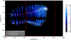 |
Fig. 1 Integrated brightness map around the O I 130.4 nm and 135.6 nm auroral features derived from UVS measurements obtained during the Juno PJ34 flyby. The map includes photons collected with the wide and narrow slit of the UVS instrument. The magenta and dashed contours mark the main auroral regions revealed by these observations. The dashed yellow polygon marks a small manually selected region we only use to illustrate an example UVS spectrum in Fig. 2. |
3 Juno/UVS observations
The Juno spacecraft performed a close flyby of Ganymede during PJ34 on 7 June 2021, providing the highest-resolution UV measurements of the moon obtained since the Galileo era. During this encounter, the UVS instrument collected UV spectra (68−210 nm) using its spin-scan observing mode, which yielded spatially resolved photon lists along the so-called dog-bone slit of the instrument (Davis et al. 2011; Gladstone et al. 2017). The same UVS dataset was used in our previous auroral study (Benmahi et al. 2025); we reorganized the calibrated photon events into latitude-longitude-wavelength cubes with a sampling of 1° and 0.1 nm, which was tailored to the retrieval of the surface reflectance.
To improve the surface coverage of Ganymede by the slit sweep, we retained the photons collected through wide parts of the slit (with a spectral resolution of ∼ 2.6 nm) and through those from the narrow slit. Since the photons measured with the narrow slit have a finer spectral resolution, they were normalized (in photon counts and spectral resolution) to match those measured with the wide slits before they were combined. From these data cubes, we reconstructed maps of the Ganymede UV brightness in the 125−210 nm spectral range. These maps include auroral emissions dominated by the O I lines at 130.4 nm and 135.6 nm and the solar continuum reflected from the icy surface of Ganymede. The integrated brightness map between 125 nm and 140 nm, shown at a high spatial resolution in Fig. 1, clearly reveals the auroral ovals of Ganymede that are produced by excited atomic oxygen following collisions between precipitating electrons and atmospheric particles.
As an illustration, Fig. 2 shows a UVS spectrum extracted from the spectral cube in the region that is arbitrarily delimited by the yellow polygon centered at a longitude of −30° and a latitude of 40°. The O I emission lines at 130.4 nm and 135.6 nm are clearly visible, superimposed on the solar continuum reflected from the surface in the 125−210 nm range. In the same figure, we also show the solar flux spectrum in the [125 nm; 210 nm] range, measured at 1 AU and taken from Curdt et al. (2001,2004). We used this spectrum to fit the solar continuum reflected from the Ganymede surface and observed by Juno/UVS and rescaled it to match a low solar activity phase and a heliocentric distance of ∼ 5.2 AU, which corresponds to the distance between the Sun and Ganymede.
The apparent feature near 133.5 nm in the solar spectrum taken from Curdt et al. (2001,2004) (see Fig. 2) corresponds to the solar C II doublet and not to a shifted OI line. The solar OI(135.6 nm) component is intrinsically extremely weak (an intensity ratio of ∼ 0.02 relative to OI(130.4 nm)), whereas in the auroral regions of Ganymede, the OI(135.6 nm) emission is strongly enhanced by electron-impact excitation of O2, which makes the auroral doublet clearly distinguishable above the reflected continuum.
To accurately interpret the observations and model the reflection of solar radiation by the surface, we also calculated the emission angle and the solar zenith angle (SZA) for each point at the surface of Ganymede observed by Juno/UVS. These two geometric parameters, shown in the maps of Figs. A.1 and A.2, allowed us to identify areas that were well illuminated and/or observed at low incidence angles. These are favorable conditions for precise measurements of the surface reflectance.
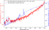 |
Fig. 2 Example of a UVS spectrum showing the reflected solar continuum and the solar reference spectrum we used. The UVS spectrum (in red) was extracted from the spectral cube within the yellow polygon shown in Fig. 1, centered at longitude −30° and latitude 40°. The incident solar flux spectrum (in blue), originally measured at 1 AU and already representative of minimum solar activity (Curdt et al. 2001, 2004), was only rescaled to the heliocentric distance of ∼ 5.2 AU, corresponding to the separation of the Sun and Ganymede. |
4 Method
Our objective was to map the surface reflectance of Ganymede as a function of wavelength based on UV observations acquired by the Juno/UVS instrument. To do this, we extracted the UV spectrum measured by Juno/UVS during PJ34 for each geographic position (longitude and latitude) in the sunlit region of the satellite (see the example in Fig. 2).
Benmahi et al. (2025) showed that the reflectance in sunlit auroral regions remains approximately constant within the 125–140 nm interval for a given geographic position, but strongly varies spatially across the surface. Beyond 140 nm, the spectral slope of the reflected solar continuum differs from that of the incident solar spectrum (see Fig. 2), which indicates that the surface reflectance depends on the wavelength in this range.
We investigated this spectral variability in the [140 nm, 205 nm] range and deliberately excluded the 125−140 nm spectral interval, which is affected by the oxygen auroral emission lines. Because the reflectance evolves relatively slowly in this spectral domain (Molyneux et al. 2020, 2022) and to improve the signal-to-noise ratio of UVS spectra, we divided the interval into seven sub-bands: [140 nm, 150 nm], [150 nm, 160 nm], [160 nm, 170 nm], [170 nm, 175 nm], [175 nm, 185 nm], [185 nm, 195 nm], and [195 nm, 205 nm].
For each position (longitude and latitude), the reflectance was determined independently within each of these sub-bands by fitting the reflected solar continuum using our UV radiative transfer model (Benmahi et al. 2025). This model takes the local viewing geometry into account, including the emission angle and solar zenith angle. Reflectance is treated as a free parameter in the model, and the fit is evaluated using the reduced χ2, which allowed us to construct a likelihood distribution as a function of the tested reflectance value. The optimal reflectance corresponds to the maximum of this distribution, and the 1σ uncertainty is derived from the width of a Gaussian fit to the likelihood curve.
The emission angle and the solar zenith angle (SZA) (see Figures A.1 and A.2) were computed at each geographic position using the Juno SPICE kernels. The uncertainties associated with these angles depend on two factors: (i) the UVS integration time per pixel, and (ii) the spatial sampling adopted in the reconstructed maps. In our case, each surface element was observed with an effective integration time of ∼ 18 ms and the spectral cubes were sampled at 1° × 1° in longitude and latitude. Under these conditions, the mean uncertainties were ∼ 0.07° for the emission angle and ∼ 0.03° for the SZA. When propagated through the radiative transfer model, these values resulted in a reflectance uncertainty of ≲ 0.08%, which is negligible compared to the typical ∼ 20% uncertainties derived from the likelihood fitting. These geometrical uncertainties were therefore not included in the reflectance maps.
To further quantify the geometric effects, we performed a sensitivity test showing that a variation of 10° in SZA can modify the retrieved reflectance by up to ∼ 13%. This confirmed that the reflectance is sensitive to local illumination conditions and justified the use of spatially resolved values of SZA (and emission angle) in the radiative transfer fitting at each geographic position.
This approach enables an accurate modeling of the reflected solar flux without requiring additional time-dependent adjustments. The use of wide spectral subintervals (5 to 10 nm spectral windows) ensured that the continuum fit was not significantly affected by narrow absorption features due to potential atmospheric or surface contaminants. To increase the signal-to-noise ratio and reduce the computational cost, we applied a spatial convolution to the final spectral cube using a latitude-longitude window of 10° × 10°. The spatial sampling of the cube was then degraded accordingly onto a 10° × 10° grid in longitude and latitude. The same spatial convolution and sampling reduction were also applied to the maps of emission angles and solar zenith angles to ensure full consistency with the spectral data. By applying this method to all observed positions in the sunlit regions, we obtained seven 2D maps of the Ganymede surface reflectance, each corresponding to one of the defined spectral subintervals.
5 Results and discussion
The surface reflectance we mapped implicitly contains information about the chemical and physical processes that modify the Ganymede surface. The spectral variability of this reflectance might arise from the differential absorption of UV photons by specific chemical compounds in the ice, whose absorption efficiency varies with wavelength. Conversely, a local increase in the reflectance might result from physical changes in the surface texture, such as variations in the ice grain size. These variations are not solely due to magnetospheric irradiation that fragments the ice, but rather to a combination of processes, including preferential sputtering of small grains (Cassidy et al. 2013) and cold-trapping effects in polar regions that retain finer particles (Molyneux et al. 2022). The reflectance maps presented below should therefore be interpreted as the combined result of (i) absorption by radiolytic species or other chemical contaminants, and (ii) intrinsic properties of the ice, including its spatial distribution, porosity, and grain size, all of which are modulated by magnetospheric irradiation, impact gardening, and thermal redistribution processes across the surface (Ligier et al. 2019; Mura et al. 2020; King & Fletcher 2022).
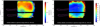 |
Fig. 3 Left: surface reflectance map of Ganymede in the spectral interval [140 nm, 150 nm], obtained by fitting the reflected solar continuum. This reflectance map was derived from the Juno/UVS spectral cube, convolved at low spatial resolution using a latitude-longitude window of 10° × 10°. Right: associated 1σ uncertainty map, expressed as a percentage of the fitted value at each latitude-longitude position. |
5.1 Retrieval of reflectance maps with a low spatial resolution
Our method for projecting the observed emissions onto the Ganymede (latitude and longitude) sampling grid relies on a hemisphere-separated projection approach. This technique creates a data gap in the equatorial region (at a latitude of between −5° and +5°) in which flux values are missing (see Fig. 1). Consequently, the values retrieved within this narrow equatorial band do not correspond to direct measurements, but result from the spatial convolution applied to the spectral cube. This region was therefore masked in all reflectance maps we present here.
In the sunlit region in which the reflectance was mapped, higher uncertainties are observed near the edges of the map. This is explained by strong emission and large solar zenith angles in these regions (see Figs. A.1 and A.2), which reduce the accuracy of the reflectance determination.
Figure 4 presents the surface reflectance maps we retrieved in the spectral intervals [150 nm, 160 nm],[160 nm, 170 nm], [170 nm, 175 nm], [175 nm, 185 nm], [185 nm, 195 nm], and [195 nm, 205 nm], derived from the same spectroscopic cube spatially convolved with a 10° × 10° window. The corresponding uncertainty maps, not shown here, have comparable characteristics to those obtained in the [140 nm, 150 nm] spectral interval (see Fig. 3).
The surface reflectance maps of Ganymede we retrieved for all spectral intervals we studied reveal a pronounced hemispheric inhomogeneity on either side of the satellite equator, with a limited but consistent correlation with the auroral emission structures. A progressive variation in the average reflectance with wavelength is also observed, which confirms the spectral dependence we highlighted. The analysis of these maps further supports the hypothesis that UV reflectance and magnetospheric irradiation are linked, particularly in the auroral regions that are exposed to intense electron precipitation. These results complement the reflectance map obtained in the [140−150 nm] interval shown in Fig. 3, and they confirm the robustness of our method over a broad spectral range. Figures 3 and 4 display the reflectance maps for each spectral interval and can be used as input for auroral radiative transfer models or for comparisons with multiwavelength observations such as those planned with Juice/UVS.
Our maps also display clear spatial similarities with the reflectance ratio maps derived by Molyneux et al. (2022) between the 190−210 nm and 150−170 nm bands. The quantity retrieved in their work, however, is a reflectance ratio of two spectral intervals, whereas we derived an absolute reflectance from radiative transfer fitting. These two quantities are therefore not directly comparable, and residual maps cannot be meaningfully constructed. The agreement between the two studies thus lies in the spatial distribution of absorptive regions and not in the magnitude of the reflectance. This consistency supports the robustness of our method for retrieving the Ganymede surface reflectance using UV spectral observations.
The reflectance in the entire sunlit region is higher at northern high latitudes above 30° N, with a peak value of ∼ 0.040 ± 0.008 at longitude =−65° and latitude =45°. Toward midlatitudes, between 30° S and 30° N, the reflectance is significantly lower, with values as low as ∼ 0.004 ± 0.0008, which is ten times lower than the values found at high northern latitudes. These low reflectance values, although unusual for planetary ices, remain within plausible physical limits. For instance, the far-UV reflectance levels of highly volatile-rich bituminous coals are as low as ∼ 0.004 between 140 and 150 nm, as shown in Fig. 1 of Hendrix et al. (2016), which is consistent with the lowest values we retrieved at midlatitudes. South of ∼ 40° S, no UVS photons were recorded during PJ34 (see Fig. 1), and the few values that appear in some reflectance maps below 40° S result solely from interpolation during plotting. These values do not correspond to actual measurements and were therefore masked in the final version of the figures.
The global reflectance decreases throughout the surface we studied over the [140 nm, 175 nm] range and then increases beyond 175 nm (see Figs. 3 and 4). Molyneux et al. (2020) investigated the spectral reflectance of the Ganymede disk using UV observations from HST. They found a similar but moderate decrease in reflectance (from ∼ 0.04 to ∼ 0.02) between 140 nm and 170 nm in the leading and trailing hemispheres1, followed by a stronger increase in the leading hemisphere and a more moderate rise in the trailing hemisphere beyond 175 nm. Although our reflectance maps are spatially resolved, the values retrieved by spectral fitting of Juno/UVS observations using our UV radiative transfer model are globally consistent with those reported by (Molyneux et al. 2020).
The observed inhomogeneity in the Ganymede surface reflectance might be linked to several processes identified in previous studies. For instance, Trumbo et al. (2023) showed that radiolytic production of UV-absorbing compounds such as H2O2 is modulated by the flux of charged particles, which might darken some regions in this spectral domain. Conversely, Molyneux et al. (2020) and Bockelée-Morvan et al. (2024) demonstrated that irradiation-driven grain-size reduction in water ice can increase the UV reflectance. The spatial variability we observe in the Ganymede surface reflectance might thus result from the competition between these opposing effects, modulated by the topology of the magnetic field on Ganymede and the orientation of its surface relative to the incoming Jovian plasma (see also Teolis et al. 2017; Tosi et al. 2024).
Finally, no clear correlation is observed between the surface reflectance structures and the visible surface features on Ganymede, regardless of whether in dark or bright regions, because the spatial resolution we adopted for this part of the study is relatively low. For this reason, and to better investigate possible correlations between the Ganymede surface reflectance, visible geological features, and auroral emission structures, we reprocessed the spectral data cube to improve the spatial resolution of the observations.
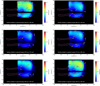 |
Fig. 4 Surface reflectance maps of Ganymede in the following six spectral intervals: [150 nm, 160 nm], [160 nm, 170 nm], [170 nm, 175 nm], [175 nm, 185 nm],[185 nm, 195 nm], and [195 nm, 205 nm]. The reflectance was obtained by fitting the reflected solar continuum, using spectra extracted from the Juno/UVS spectral cube, spatially convolved with a latitude-longitude window of 10° × 10°. These maps complete the reflectance map in the [140 nm, 150 nm] interval shown in Fig. 3, and allow us to analyze the UV reflectance on the Ganymede surface spectrally and spatially. |
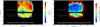 |
Fig. 5 Left: surface reflectance map of Ganymede in the spectral interval [140 nm, 150 nm], obtained by fitting the reflected solar continuum. This reflectance map was derived from the Juno/UVS spectral cube convolved at high spatial resolution using a latitude-longitude window of 5° × 5°. Right: uncertainty map associated with the reflectance, expressed as a percentage of the fit value at each (latitude, longitude) position, using the same spatial resolution as for the top map. |
5.2 Retrieval of reflectance maps with a high spatial resolution
As in the previous section, we produced a surface reflectance map, but this time, by convolving the spectral data cube with a smaller latitude-longitude window of 5° × 5°. Although the signal-to-noise ratio decreased, this second mapping provided a higher level of detail in the observed structures. Figure 5 shows the reflectance map obtained in the [140 nm, 150 nm] spectral interval, along with the uncertainty map calculated at the same spatial resolution. As highlighted in the previous section (see Section 5.1), it is important to reiterate that the reflectance values retrieved within the equatorial band between −5° and +5° latitude do not originate from reliable measurements. Instead, they are artifacts introduced by the spatial convolution of the spectral cube. They should therefore not be considered physically meaningful.
Compared to Fig. 3, this new high-resolution map reveals finer spatial structures, with a consistently higher reflectance observed at northern high latitudes, above 30° N. Several local reflectance maxima are identified, including one at longitude = −65° and latitude =45° with a reflectance of 0.080 ± 0.020, and another at longitude =50° and latitude =45° with a reflectance of 0.080 ± 0.016. These peaks show reasonable uncertainties, which supports their robustness. Interestingly, these locations coincide with regions that were previously identified as ice rich based on infrared observations. In particular, Mura et al. (2020) reported several ice-rich craters near −65° longitude and above 45° latitude (see their Fig. 9), and Ligier et al. (2019) highlighted a high concentration of water ice near 50° longitude and 55° latitude (see their Fig. 10b). This consistency supports the physical reliability of the observed UV reflectance enhancements in these areas. In contrast, the peak at longitude =20°, latitude =80° with a reflectance of 0.060 ± 0.051 appears to be less robust due to a large uncertainty that is linked to a high SZA and a highly grazing emission angle that approaches 90°.
The high reflectance observed at high latitudes is consistent with the findings of Trumbo et al. (2023), who reported no significant enhancement in IR absorption by H2O2 in the trailing hemisphere at mid- and polar latitudes. This does not necessarily imply that H2O2 is absent or negligible in the UV, however. Both H2O and H2O2 are known to be relatively dark in the 140−150 nm range (Molyneux et al. 2020), and variations in reflectance might equally result from changes in the ice grain size, porosity, or microstructure and not from composition alone. In this context, the enhanced reflectance at high latitudes is more likely associated with the distribution of water ice itself, which is known to be more concentrated in the polar regions, as reported in previous studies (Khurana et al. 2007; Stephan et al. 2020; Mura et al. 2020).
In addition, the orbital velocity of Ganymede around Jupiter is lower than the rotational speed of the Jupiter plasma disk (Kivelson et al. 2007), and the trailing hemisphere therefore lies downstream of the corotating Jovian plasma flow. While the intrinsic magnetosphere of Ganymede significantly shields from direct plasma impact, especially at low latitudes, some energetic particles can still access the surface at high latitudes where the magnetic field lines are open or distorted (Poppe et al. 2018). As suggested by Molyneux et al. (2020) and modeled by Poppe et al. (2018), this magnetospheric irradiation might contribute to reducing the grain size of surface ice in polar regions, thereby enhancing the UV reflectance through increased scattering.
A similar observation covering the leading hemisphere would be crucial to determine whether radiolytic production is stronger there and might in turn reduce reflectance. Although our observations do not fully cover this hemisphere, the small portion included near 47° longitude shows that reflectance is also high in this region.
Finally, the spectral impact of radiolytic processing might differ significantly between the UV and infrared domains. For instance, Bockelée-Morvan et al. (2024) observed localized decreases in IR reflectance, which they attributed to the presence of radiolytic products such as H2O2. These compounds are known to absorb efficiently in the IR, but also exhibit absorption features in the UV (e.g., Trumbo et al. 2023; Molyneux et al. 2020). The extent to which each radiolytic species affects the UV reflectance remains poorly constrained, however, and it likely depends on their abundance and distribution.
In our study, the UV reflectance is generally higher in regions that are subjected to intense magnetospheric precipitation. While the physical mechanisms behind this trend remain uncertain, it might result from irradiation-induced changes in the surface ice properties, such as the grain size or structural state. Further laboratory studies and upcoming observations from missions such as Juice and Europa Clipper will be crucial to understand these effects better.
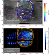 |
Fig. 6 Comparison of the surface reflectance map in the [140 nm, 150 nm] interval with two different datasets. Top: comparison with the visible surface map of Ganymede, highlighting geological features. Bottom: comparison with the total brightness map of the atomic oxygen auroral emission lines at 130.4 nm and 135.6 nm, observed during the Juno PJ34 flyby. The dashed magenta polygons indicate the main auroral regions identified from the UVS observations. |
5.3 Comparison of the reflectance maps with the auroral brightness and visible surface maps
Figure 6 illustrates the superposition of the surface reflectance map obtained in the [140 nm, 150 nm] spectral interval (shown in Fig. 5), the auroral brightness maps integrated between 125 and 140 nm (shown in Fig. 1), and the visible map of the Ganymede surface. The objective of this comparison is to qualitatively assess possible correlations between UV reflectance, visible geological structures, and auroral emissions, the latter being direct tracers of the interaction between magnetospheric plasma and the satellite surface.
The comparison between the UV reflectance map and the visible surface morphology reveals no systematic correlation with the large-scale dark or bright terrains commonly identified in the optical domain. Nevertheless, several local maxima in UV reflectance appear to be spatially consistent with regions that were previously identified as rich in water ice. In particular, the reflectance peaks at longitude =−65° and latitude =45° (with a reflectance of 0.080 ± 0.020) and at longitude =50° and latitude =45° (with a reflectance of 0.080 ± 0.016) lie within the latitude range (>40° N), where JIRAM infrared observations reported stronger water-ice signatures (Mura et al. 2020). They are also close to crater-rich areas located around longitude = −65° and latitude =45°. The geographical consistency of the UV local maxima and regions that were previously associated with enhanced surface-ice content supports the physical plausibility of these reflectance enhancements, even though the current reflectance maps do not provide a sufficient spatial resolution for a one-to-one crater identification.
In contrast, no clear enhancement is detected around the Tros crater (longitude =30°, latitude =15°), despite its prominent appearance in visible imagery and its ice-rich nature (Bockelée-Morvan et al. 2024). This absence of a correlation might indicate spatial variability in the surface properties such as grain size or composition that is not captured solely by morphology or brightness in the visible or near-infrared because magnetospheric precipitation is weaker in these regions (Poppe et al. 2018).
At southern latitudes, additional reflectance peaks are observed near longitude =−65°,=−20°, and 35°, below latitude =−10°, with reflectance values of 0.030 ± 0.018, 0.025 ± 0.010, and 0.020 ± 0.013, respectively. Several of these features lie close to cratered regions, such as We-ila (longitude =−70° and latitude =12°), Enkidu (longitude =−35° and latitude =26°), and Serapis (longitude =44° and latitude =12°), although the higher uncertainties in these southern areas (see Fig. 6) warrant a cautious interpretation. These results suggest that while large-scale surface morphology alone does not control the UV reflectance, localized features, particularly ice-rich craters at high latitudes, might affect the reflectance through a higher ice content or finer grain sizes, which might be linked to magnetospheric precipitation processes.
On the other hand, the comparison with auroral brightness maps does not reveal significant correlations. While the main auroral emission arcs appear to partially agree with regions of high reflectance on either side of the equator, no clear geometric correspondence is observed. In contrast, the peak of atomic oxygen emission around longitude =−75° and latitude =50° coincides with a region of a stronger reflectance. In these areas, a portion of the precipitating electrons produces excited atomic oxygen (O*), which causes the observed UV auroral emissions (Greathouse et al. 2022). Higher-energy electrons, however, might traverse the atmosphere without significant interaction and reach the Ganymede surface, where they alter the structure of the ice. In particular, energetic irradiation can induce a transition from crystalline to amorphous ice or modify the size distribution of fine grains (Teolis et al. 2017; Molyneux et al. 2020). These physical effects, which depend on local temperature and sputtering rates, might lead to an increased UV reflectance by enhancing the scattering efficiency. The overall outcome remains complex, however, and likely involves a combination of competing processes that are not yet fully understood.
6 Conclusions
We presented a spectral 2D mapping of the UV reflectance of the Ganymede dayside surface based on observations from the UVS instrument on board the Juno mission during the PJ34 flyby. Using a non-LTE UV radiative transfer model (Benmahi et al. 2025), we fit the solar continuum reflected by the surface to retrieve the reflectance in several spectral intervals between 140 and 205 nm, taking the local illumination geometry into account.
Our results extend the work of Benmahi et al. (2025) and Molyneux et al. (2022) and demonstrated that surface reflectance varies significantly geographically in the broader UV range [140–205 nm], in addition to the previously analyzed 125–140 nm interval (Benmahi et al. 2025). Furthermore, this study revealed that the reflectance also varies spectrally, which suggests a wavelength dependence that might be linked to the composition, porosity, or grain-size distribution of the surface ice. These properties might be affected by magnetospheric irradiation processes, which can fragment ice grains (increasing reflectance) and produce UV-absorbing radiolytic compounds (decreasing reflectance), as discussed by Molyneux et al. (2022), Trumbo et al. (2023), and Bockelée-Morvan et al. (2024).
In particular, we identified reflectance peaks in auroral regions at midlatitudes, which might reflect the dominant effect of the ice-grain structure alteration induced by energetic magnetospheric particle precipitation. These results support the hypotheses formulated by Molyneux et al. (2022) regarding the role of auroral precipitation in the physical alteration of the surface. The absence of marked absorption features in the leading hemisphere, observable here only at longitudes greater than ∼ 45°, suggests that radiolytic products such as H2O2, OH, or O3, which are known to be dark in the far-UV but do not exhibit distinctive spectral signatures in this range, are not readily detectable with our current dataset and resolution.
This spectral reflectance mapping represents a significant advance for the modeling of the auroral emission of Ganymede. It will enable a better interpretation of future UV observations by the Juice/UVS instrument, particularly in dayside auroral regions, in which solar radiation reflection plays a critical role. Extending this method to currently unobserved areas, especially the leading hemisphere, will be essential for constraining the effect of radiolysis on the satellite surface better and for quantifying the longitudinal asymmetries that might be induced by magnetospheric interaction.
Acknowledgements
B. Benmahi and V. Hue acknowledge support from the French government under the France 2030 investment plan, as part of the Initiative d’Excellence d’Aix-Marseille Université – A*MIDEX AMX-22-CPJ-04. B. Benmahi and V. Hue acknowledge the support of CNES to the Juno and Juice missions. B.B. is a Research Associate of the Fonds de la Recherche Scientifique – FNRS.
References
- Allegrini, F., Bagenal, F., Ebert, R. W., et al. 2022, Geophys. Res. Lett., 49, e2022GL098682 [NASA ADS] [CrossRef] [Google Scholar]
- Benmahi, B., 2022, PhD thesis, Université de Bordeaux, France [Google Scholar]
- Benmahi, B., Bonfond, B., Benne, B., et al. 2024a, A&A, 685, A26 [Google Scholar]
- Benmahi, B., Bonfond, B., Benne, B., et al. 2024b, A&A, 691, A91 [NASA ADS] [CrossRef] [EDP Sciences] [Google Scholar]
- Benmahi, B., Hue, V., Vorbuger, A., et al. 2025, A&A, in press, https://doi.org/10.1051/0004-6361/202556996 [Google Scholar]
- Benne, B., Benmahi, B., Dobrijevic, M., et al. 2024, A&A, 686, A22 [NASA ADS] [CrossRef] [EDP Sciences] [Google Scholar]
- Bockelée-Morvan, D., Lellouch, E., Poch, O., et al. 2024, A&A, 681, A27 [NASA ADS] [CrossRef] [EDP Sciences] [Google Scholar]
- Carnielli, G., Galand, M., Leblanc, F., et al. 2019, Icarus, 330, 42 [Google Scholar]
- Cassidy, T. A., Paranicas, C. P., Shirley, J. H., et al. 2013, Planet. Space Sci., 77, 64 [Google Scholar]
- Curdt, W., Brekke, P., Feldman, U., et al. 2001, A&A, 375, 591 [NASA ADS] [CrossRef] [EDP Sciences] [Google Scholar]
- Curdt, W., Landi, E., & Feldman, U., 2004, A&A, 427, 1045 [NASA ADS] [CrossRef] [EDP Sciences] [Google Scholar]
- Davis, M. W., Gladstone, G. R., Greathouse, T. K., et al. 2011, in Radiometric Performance Results of the Juno Ultraviolet Spectrograph (Juno/UVS), eds. H. A. MacEwen, & J. B. Breckinridge (San Diego, California, USA), 814604 [Google Scholar]
- Gladstone, G. R., Persyn, S. C., Eterno, J. S., et al. 2017, Space Sci. Rev., 213, 447 [Google Scholar]
- Greathouse, T. K., Gladstone, G. R., Molyneux, P. M., et al. 2022, Geophys. Res. Lett., 49, e2022GL099794 [NASA ADS] [CrossRef] [Google Scholar]
- Hall, D. T., Feldman, P. D., McGrath, M. A., & Strobel, D. F., 1998, ApJ, 499, 475 [NASA ADS] [CrossRef] [Google Scholar]
- Hansen, C. J., Bolton, S., Sulaiman, A. H., et al. 2022, Geophys. Res. Lett., 49, e2022GL099285 [Google Scholar]
- Hendrix, A. R., Vilas, F., & Li, J.-Y. 2016, Meteor. Planet. Sci., 51, 105 [Google Scholar]
- Khurana, K. K., Pappalardo, R. T., Murphy, N., & Denk, T., 2007, Icarus, 191, 193 [NASA ADS] [CrossRef] [Google Scholar]
- King, O., & Fletcher, L. N., 2022, J. Geophys. Res.: Planets, 127, e2022JE007323 [NASA ADS] [CrossRef] [Google Scholar]
- Kivelson, M. G., Bagenal, F., Kurth, W. S., et al. 2007, in Jupiter, 513 [Google Scholar]
- Leblanc, F., Oza, A. V., Leclercq, L., et al. 2017, Icarus, 293, 185 [NASA ADS] [CrossRef] [Google Scholar]
- Ligier, N., Paranicas, C., Carter, J., et al. 2019, Icarus, 333, 496 [NASA ADS] [CrossRef] [Google Scholar]
- Lilensten, J., Kofman, W., Wisemberg, J., Oran, E. S., & DeVore, C. R., 1989, Ann. Geophys., 7, 83 [NASA ADS] [Google Scholar]
- Molyneux, P. M., Nichols, J. D., Bannister, N. P., et al. 2018, J. Geophys. Res.: Space Phys., 123, 3777 [Google Scholar]
- Molyneux, P. M., Nichols, J. D., Becker, T. M., Raut, U., & Retherford, K. D., 2020, J. Geophys. Res.: Planets, 125, e2020JE006476 [Google Scholar]
- Molyneux, P. M., Greathouse, T. K., Gladstone, G. R., et al. 2022, Geophys. Res. Lett., 49, e2022GL099532 [Google Scholar]
- Mura, A., Adriani, A., Sordini, R., et al. 2020, J. Geophys. Res.: Planets, 125, e2020JE006508 [Google Scholar]
- Poppe, A. R., Fatemi, S., & Khurana, K. K., 2018, J. Geophys. Res.: Space Phys., 123, 4614 [NASA ADS] [CrossRef] [Google Scholar]
- Stephan, K., Hibbitts, C. A., & Jaumann, R., 2020, Icarus, 337, 113440 [NASA ADS] [CrossRef] [Google Scholar]
- Teolis, B. D., Plainaki, C., Cassidy, T. A., & Raut, U., 2017, J. Geophys. Res.: Planets, 122, 1996 [NASA ADS] [CrossRef] [Google Scholar]
- Tosi, F., Roatsch, T., Galli, A., et al. 2024, Space Sci. Rev., 220, 59 [Google Scholar]
- Trumbo, S. K., Brown, M. E., Bockelée-Morvan, D., et al. 2023, Sci. Adv., 9, eadg3724 [NASA ADS] [CrossRef] [Google Scholar]
- Vorburger, A., Fatemi, S., Carberry Mogan, S. R., et al. 2024, Icarus, 409, 115847 [NASA ADS] [CrossRef] [Google Scholar]
- Waite, J. H., Greathouse, T. K., Carberry Mogan, S. R., et al. 2024, J. Geophys. Res.: Planets, 129, e2023JE007859 [NASA ADS] [CrossRef] [Google Scholar]
The leading hemisphere corresponds to the forward-facing side of Ganymede along its orbit, and the trailing hemisphere refers to the opposite side. In our maps, these hemispheres are centered around 90° and −90° longitude, respectively.
Appendix A Viewing and illumination geometry
The retrieval of Ganymede’s surface reflectance requires an accurate determination of the local viewing and illumination conditions for each observation point. Figures A.1 and A.2 therefore present, respectively, the maps of the emission angle and the solar zenith angle (SZA) over the sunlit region observed during PJ34. These two geometric parameters are computed for each latitude-longitude bin using Juno’s SPICE kernels.
The emission angle indicates how close the line of sight is to the surface normal. Low values (near 0°) correspond to observations nearly perpendicular to the surface and are most favorable for constraining reflectance, whereas high values indicate grazing viewing geometries. Similarly, the SZA characterizes the level of solar illumination: low values correspond to strong solar incidence (near local noon), while high values indicate weak or grazing illumination near the terminator.
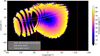 |
Fig. A.1 Map of emission angles at Ganymede’s surface, defined as the angle between the local surface normal and the viewing direction of the UVS instrument. Low values (in blue) correspond to regions observed nearly perpendicularly to the surface, while high values (in yellow) indicate more oblique observations, which are less favorable for accurate surface albedo measurements. |
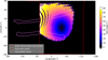 |
Fig. A.2 Map of the solar zenith angle at Ganymede’s surface, defined as the angle between the local surface normal and the direction of the Sun. Low values (in blue) indicate strongly illuminated regions near the solar zenith, while high values (in white) correspond to areas near the terminator, receiving weak or grazing solar illumination. |
Appendix B Influence of atmospheric H2 O abundance on the reflectance retrieving
To assess the impact of the H2O density on the determination of surface reflectance through the fitting of the reflected solar continuum in subsolar regions, we conducted a sensitivity study. For this purpose, we selected a location outside the subsolar region, at coordinates longitude =−77° and latitude =45°. At this position, we artificially modified the H2O density in our atmospheric model before performing the radiative transfer simulation.
These modifications consisted in multiplying the vertical abundance profile of H2O by a given factor. In this study, we applied the following scaling factors: 1, 2, 5, 10, 50, 100, 500, and 1000. For each case, we computed the surface reflectance by fitting the reflected solar continuum in the spectral interval [140 nm, 150 nm]. At the selected location, the reflectance retrieved from the map in Fig. 5 is approximately ∼ 0.08. The goal is to determine at which scaling factor the reflectance begins to significantly deviate from this reference value.
This analysis allows us to evaluate whether such variations in H2O density are realistic and to what extent the effect of H2O can be neglected in subsolar regions, where the near-surface H2O density is typically 8 to 12 times higher than that of O2.
Figure B.1 shows the evolution of reflectance as a function of the scaling factor applied to the H2O abundance profile. The results clearly indicate that the reflectance begins to change significantly only when the H2O density is increased by a factor of 100 or more. This suggests that, in subsolar regions, the actual H2O abundance is insufficient to significantly affect the reflectance retrieval performed in this study. Therefore, using an atmospheric model based on average abundance profiles for each chemical species is fully justified within the framework of our spectral mapping method for surface reflectance.
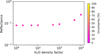 |
Fig. B.1 Evolution of the reflectance in the [140 nm, 150 nm] range as a function of the scaling factor applied solely to the vertical abundance profile of H2O, and as a function of the reflectance uncertainty [in%]. |
All Figures
|
Fig. 1 Integrated brightness map around the O I 130.4 nm and 135.6 nm auroral features derived from UVS measurements obtained during the Juno PJ34 flyby. The map includes photons collected with the wide and narrow slit of the UVS instrument. The magenta and dashed contours mark the main auroral regions revealed by these observations. The dashed yellow polygon marks a small manually selected region we only use to illustrate an example UVS spectrum in Fig. 2. |
| In the text | |
|
Fig. 2 Example of a UVS spectrum showing the reflected solar continuum and the solar reference spectrum we used. The UVS spectrum (in red) was extracted from the spectral cube within the yellow polygon shown in Fig. 1, centered at longitude −30° and latitude 40°. The incident solar flux spectrum (in blue), originally measured at 1 AU and already representative of minimum solar activity (Curdt et al. 2001, 2004), was only rescaled to the heliocentric distance of ∼ 5.2 AU, corresponding to the separation of the Sun and Ganymede. |
| In the text | |
|
Fig. 3 Left: surface reflectance map of Ganymede in the spectral interval [140 nm, 150 nm], obtained by fitting the reflected solar continuum. This reflectance map was derived from the Juno/UVS spectral cube, convolved at low spatial resolution using a latitude-longitude window of 10° × 10°. Right: associated 1σ uncertainty map, expressed as a percentage of the fitted value at each latitude-longitude position. |
| In the text | |
|
Fig. 4 Surface reflectance maps of Ganymede in the following six spectral intervals: [150 nm, 160 nm], [160 nm, 170 nm], [170 nm, 175 nm], [175 nm, 185 nm],[185 nm, 195 nm], and [195 nm, 205 nm]. The reflectance was obtained by fitting the reflected solar continuum, using spectra extracted from the Juno/UVS spectral cube, spatially convolved with a latitude-longitude window of 10° × 10°. These maps complete the reflectance map in the [140 nm, 150 nm] interval shown in Fig. 3, and allow us to analyze the UV reflectance on the Ganymede surface spectrally and spatially. |
| In the text | |
|
Fig. 5 Left: surface reflectance map of Ganymede in the spectral interval [140 nm, 150 nm], obtained by fitting the reflected solar continuum. This reflectance map was derived from the Juno/UVS spectral cube convolved at high spatial resolution using a latitude-longitude window of 5° × 5°. Right: uncertainty map associated with the reflectance, expressed as a percentage of the fit value at each (latitude, longitude) position, using the same spatial resolution as for the top map. |
| In the text | |
|
Fig. 6 Comparison of the surface reflectance map in the [140 nm, 150 nm] interval with two different datasets. Top: comparison with the visible surface map of Ganymede, highlighting geological features. Bottom: comparison with the total brightness map of the atomic oxygen auroral emission lines at 130.4 nm and 135.6 nm, observed during the Juno PJ34 flyby. The dashed magenta polygons indicate the main auroral regions identified from the UVS observations. |
| In the text | |
|
Fig. A.1 Map of emission angles at Ganymede’s surface, defined as the angle between the local surface normal and the viewing direction of the UVS instrument. Low values (in blue) correspond to regions observed nearly perpendicularly to the surface, while high values (in yellow) indicate more oblique observations, which are less favorable for accurate surface albedo measurements. |
| In the text | |
|
Fig. A.2 Map of the solar zenith angle at Ganymede’s surface, defined as the angle between the local surface normal and the direction of the Sun. Low values (in blue) indicate strongly illuminated regions near the solar zenith, while high values (in white) correspond to areas near the terminator, receiving weak or grazing solar illumination. |
| In the text | |
|
Fig. B.1 Evolution of the reflectance in the [140 nm, 150 nm] range as a function of the scaling factor applied solely to the vertical abundance profile of H2O, and as a function of the reflectance uncertainty [in%]. |
| In the text | |
Current usage metrics show cumulative count of Article Views (full-text article views including HTML views, PDF and ePub downloads, according to the available data) and Abstracts Views on Vision4Press platform.
Data correspond to usage on the plateform after 2015. The current usage metrics is available 48-96 hours after online publication and is updated daily on week days.
Initial download of the metrics may take a while.