| Issue |
A&A
Volume 706, February 2026
|
|
|---|---|---|
| Article Number | A178 | |
| Number of page(s) | 13 | |
| Section | Stellar structure and evolution | |
| DOI | https://doi.org/10.1051/0004-6361/202453497 | |
| Published online | 10 February 2026 | |
The interdependence between density PDF, CMF, and IMF and their relation with Mach number in simulations
1
Université Paris-Saclay, Université Paris Cité CEA, CNRS, AIM 91191 Gif-sur-Yvette, France
2
Université Paris Cité, Université Paris-Saclay, CEA, CNRS, AIM F-91191 Gif-sur-Yvette, France
3
Universität Heidelberg, Zentrum für Astronomie, Institut für Theoretische Astrophysik Albert-Ueberle-Str 2 D-69120 Heidelberg, Germany
4
Univ. Grenoble Alpes, CNRS, IPAG 38000 Grenoble, France
5
Centre de Recherche Astrophysique de Lyon UMR5574, ENS de Lyon, Univ. Lyon1, CNRS, Université de Lyon 69007 Lyon, France
★ Corresponding author: This email address is being protected from spambots. You need JavaScript enabled to view it.
Received:
18
December
2024
Accepted:
29
September
2025
Abstract
Context. The initial mass function (IMF) of stars and the corresponding cloud mass function (CMF), traditionally considered universal, exhibit variations that are influenced by the local environment. Notably, these variations are apparent in the distribution’s tail, indicating a possible relationship between local dynamics and mass distribution.
Aims. Our study was designed to examine how the gas PDF, the IMF, and the CMF depend on the local turbulence within the interstellar medium (ISM).
Methods. We ran hydrodynamical simulations on small star-forming sections of the ISM under varying turbulence conditions, characterised by Mach numbers of 1, 3.5, and 10, and with two distinct mean densities. This approach allowed us to observe the effects of different turbulence levels on the formation of stellar and cloud masses.
Results. The study demonstrates a clear correlation between the dynamics of the cloud and the IMF. In environments with lower levels of turbulence likely dominated by gravitational collapse, our simulations showed the formation of more massive structures with a power-law gas PDF, leading to a top-heavy IMF and CMF. On the other hand environment dominated by turbulence result in a lognormal PDF and a Salpeter-like CMF and IMF. This indicates that the turbulence level is a critical factor in determining the mass distribution within star-forming regions.
Key words: stars: abundances / stars: formation / stars: kinematics and dynamics / stars: luminosity function / mass function / stars: massive / stars: statistics
© The Authors 2026
 Open Access article, published by EDP Sciences, under the terms of the Creative Commons Attribution License (https://creativecommons.org/licenses/by/4.0), which permits unrestricted use, distribution, and reproduction in any medium, provided the original work is properly cited.
This article is published in open access under the Subscribe to Open model. This email address is being protected from spambots. You need JavaScript enabled to view it. to support open access publication.
1. Introduction
The stellar initial mass function (IMF), defined as the number density of stars per logarithmic mass interval, dN/dlog M, has been the subject of extensive research across various settings, including the Galactic field, young clusters, star-forming regions, as well as the Galactic bulge, halo, and high-redshift galaxies. This research aims to uncover the physical principles shaping its pattern; we refer to Kroupa (2002), Chabrier (2003), and Hennebelle & Grudić (2024) for comprehensive reviews. Understanding the IMF accurately remains a critical, yet unresolved, challenge in astrophysics. The IMF is crucial for linking stellar and galactic evolution and influences the universe’s chemical composition, luminosity, and baryonic content. Additionally, many analyses of the prestellar dense core mass function (CMF) have investigated whether it mirrors the IMF, primarily because it has been proposed that they could present similar forms (see for instance André et al. 2010; Könyves et al. 2015). In particular, the exponent of the power law, α, where
 (1)
(1)
which is usually used to describe the stellar mass distribution, has been found to be comparable both for the IMF and for the CMF with typical reported values for α close to 2.35, as originally inferred by Salpeter (1955), although significantly shallower values have also been reported. In the literature, the index may also be found as ΓIMF = −α + 1.
Another important feature is the peak of the IMF which is usually observed to occur at about 0.3 M⊙. Typically, the CMF is observed to shift by a factor of 2 to 4 towards higher masses relative to the IMF (Motte et al. 1998; Testi & Sargent 1998; Johnstone et al. 2000; André et al. 2007; Alves et al. 2007; André et al. 2010; Könyves et al. 2015), although Louvet et al. (2021) claim that the peak of the CMF that has been reported is determined by the instrumental resolution. For a relation to hold between the CMF and the IMF, there must be a sufficiently accurate correlation between the mass of protostellar cores and the ultimate mass of stars. However, accurately assessing this correlation continues to be a significant challenge (e.g. Smith et al. 2009; Ntormousi & Hennebelle 2019; Smullen et al. 2020; Pelkonen et al. 2021).
The shape of the IMF in most studies is derived by constructing a histogram of stellar masses (or their logarithmic values) in equally sized bins, followed by fitting one or several functional forms. Minimising the chi-square of the fit allows for the derivation of fit parameters. In the intermediate- to high-mass regimes, the slopes derived from this method range between 0.7 and 2 when stellar masses are binned logarithmically. Although it is often stated in the literature that the derived values are consistent with the Salpeter slope within the 1σ uncertainty, the clarity of this claim is questionable (Dib 2014). An examination of the slope values in this mass regime for several clusters, which employed identical data reduction algorithms and theoretical evolutionary tracks for deriving stellar masses, suggests that the IMF slopes for these clusters do not agree within the 1σ uncertainty level (Sharma et al. 2008; Lata et al. 2010; Tripathi et al. 2014).
It is becoming increasingly evident that the density structure of the interstellar medium (ISM), where cores form, is predominantly influenced by supersonic turbulence across a broad spectrum of scales (Elmegreen & Scalo 2004; Mac Low & Klessen 2004; McKee & Ostriker 2007). A common result of this turbulence is the convergence of the density distribution towards a lognormal probability distribution function (PDF), where the dispersion exhibits a clear dependence on the Mach number (see Vazquez-Semadeni 1994; Padoan et al. 1997; Scalo et al. 1998; Ostriker et al. 1999, also see Hopkins (2013) for a more robust PDF description and Brucy et al. (2024) and Hennebelle et al. (2024) for its relation with simulation and star formation theories).
The IMF has been derived from numerical simulations using Lagrangian sink particles (e.g. Krumholz et al. 2004; Bleuler & Teyssier 2014). Several studies have been carried out along the years and early calculations include for instance Bate & Bonnell (2005), Padoan & Nordlund (2002), Tilley & Pudritz (2004), Li et al. (2004), Ballesteros-Paredes et al. (2006), Padoan et al. (2007).
Two main numerical set-ups are used to compute the IMF: isolated turbulent collapsing clumps (e.g. Bate 2009; Ballesteros-Paredes et al. 2015; Lee & Hennebelle 2018) and driven turbulence periodic boxes (e.g. Haugbølle et al. 2018; Mathew et al. 2023). In the former configuration, a turbulent velocity field is initialised and the collapsing clump is then evolved without further driving. Lee & Hennebelle (2018) have investigated the influence of the initial virial parameter, αvir, of the collapsing clump (see their Figure 7) between αvir = 0.1 to 1.5. They report that unless αvir < 0.3, the influence of α variation remains limited and the slope of the heavy tail of the IMF ΓIMF = −α + 1 remains between –0.8 and –1. The values of ΓIMF obtained with turbulent forcing tend to be steeper and closer to −1.3. Figure 9 of Haugbølle et al. (2018) reveals that between ≃2 and 10 M⊙, the stellar distribution appears to be compatible with −α + 1 ≃ −1.3. The work of Mathew et al. (2023) presents similar trends and values of −α + 1 ≃ −1.3 are also inferred (see their Figure 7). Recently, Guszejnov et al. (2022) have performed a series of numerical simulations corresponding either to periodic boxes with and without turbulent driving or to collapsing clouds. Figure 16 of Guszejnov et al. (2022) shows the difference between the various configurations. All cases have −α + 1 ≃ −1 except the turbulent driven simulation for which −α + 1 ≃ −1.3.
The reason for the differences found when turbulence is driven and when it is not driven, is not yet clear. One possibility is that they are a consequence of the density PDF as proposed in Lee & Hennebelle (2018). We recall that in the gravo-turbulent model of Hennebelle & Chabrier (2008) the inferred value of α is such that α − 1 = (n + 1)/(2n − 4), where n ≃ 3.7 is the exponent of the velocity power spectrum. To get this relation, a lognormal PDF is assumed. However, when gravitational collapse is assumed, a power-law PDF ∝ρ−3/2 develops (e.g. Kritsuk et al. 2011; Hennebelle & Falgarone 2012), and the inferred exponent for the IMF is such that α − 1 = (5n − 13)/(2n − 4).
The purpose of the present paper is to better understand the origin of the different regimes that have been inferred for the exponent α. For this purpose we present a series of high-resolution simulations in which we varied the strength of the turbulent driving, therefore producing flows at various Mach numbers. In parallel to the IMF, we examined the CMF to evaluate the extent of variation in its exponent and to determine if the exponents of the IMF and CMF are similar and exhibit comparable changes.
In the second part of the paper we present various definitions and discuss how to measure power-law exponents. The third part is devoted to the numerical set-up. In sections four, five and six, we discuss the density PDF, the CMF and the IMF, respectively. Finally, part seven concludes the paper.
2. The IMF: Definition and slope measurement
2.1. Initial mass function
The IMF as originally defined by Salpeter (1955) is the number of stars N in a volume of space V per logarithmic mass interval dlog m,
 (2)
(2)
where n is the stellar number density. While this logarithmic form is the most satisfactory representation of the mass distribution in the Galaxy, there is an alternative definition from Scalo (1986) where the mass spectrum is defined in linear mass intervals. It is then clear that
 (3)
(3)
There are several definitions for the shape of ξ, all agreeing on the fact that the tail of the distribution behaves as a power law of the form ξ(m)∝m−α, meaning that ξ(log m)∝m−α + 1. The original value proposed by Salpeter (1955) was developed on the logarithmic scale and resulted in α = 2.351 (see Chabrier 2003 for a review).
The IMF is represented as a power-law probability distribution. This classification is interesting because power-law distributions are tail-heavy. This means that their distribution of the high-mass elements retains a significant contribution to the total mass.
2.2. Tail-heavy distributions
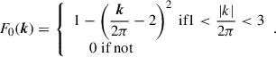
In practice, it is uncommon for empirical phenomena to follow power laws across all values of x. Typically, the power law is relevant only for values above a certain minimum xmin. We consider the IMF to be a power-law probability distribution of the form
 (4)
(4)
where C is a normalisation constant. Clearly, this expression diverges as x → 0, and therefore it cannot describe the probability of all positive values of x. Thus, a minimum value, xmin, is required and can be used to compute C assuming α > 1 as
 (5)
(5)
Once xmin is defined, one can estimate the value and respective uncertainty of the power-law index α using the maximum likelihood estimate (MLE) method as described in Clauset et al. (2009). More specifically, using the Python package qcrpowerlaw presented in Alstott et al. (2014). This method provides an accurate estimation of the index α as
![Mathematical equation: $$ \begin{aligned} \hat{\alpha } = 1+n\left[\sum ^n_{i = 1} \text{ ln} \frac{x_i}{x_{\rm min}} \right], \end{aligned} $$](/articles/aa/full_html/2026/02/aa53497-24/aa53497-24-eq6.gif) (6)
(6)
where xi is the mass of the i-th element, provided that xi > xmin. The uncertainty on α is estimated as
 (7)
(7)
where O is the mathematical notation for non-negligible. Opting for this method instead of fitting the tail of the distribution addresses the different issues in this type of analysis. Specifically, representing distributions with histograms followed by linear regression can cause inaccuracies (Clauset et al. 2009). Depicting the probability function in log-log scales does not allow the fit uncertainty to be assessed because of non-Gaussian noise. Furthermore, the bin width selection adds a complicating factor to estimating uncertainty.
In many cases, it is useful to also consider the complementary cumulative distribution function (CCDF) of a power-law distributed variable that can be denoted as
 (8)
(8)
For distributions such as the CMF and IMF, this method is especially useful because it eliminates the need for binning in plotting, as all that is to be plotted is the exact number of cores of stars above each mass, thus removing a potential source of uncertainty. However, it introduces a point of confusion; the scaling parameter appears as −α + 1, coincidentally matching the scaling in the logarithmic version of the IMF from Equation (2), but this similarity is coincidental. For the sake of clarity, Table 1 lists the equations used in the upcoming analyses and describes how their power-law tails scale. The visual representation of the CCDF is generally more robust against fluctuations due to finite sample sizes, particularly in the tail of the distribution, compared to that of the PDF. Therefore, in the subsequent analysis, the tail of the CCDF, P(x), is shown for cores and stellar particles and not the direct probability density function.
3. Numerical set-up
3.1. Simulation framework
Here we describe the hydrodynamic simulations for turbulent gas dynamics that were run using the adaptive mesh refinement (AMR) code RAMSES (Teyssier 2002). The simulations incorporate a Godunov scheme, the HLLC Riemann solver, and MINMOD slope limiter. The AMR used here has a maximum refinement level of 15 in a 10 pc box, corresponding to a minimum cell size of 63 AU. Refinement is based on the local Jeans length, ensuring it is always resolved by at least ten cells (i.e. a Jeans number of 10). AMR is active throughout the entire simulation, including the turbulence driving phase, before gravity is enabled.
3.2. Initial conditions
Our simulations commence with a straightforward set-up: a uniform-density gas field, driven by large-scale turbulence, in a periodic cubic box. The box, with side lengths of 10 pc, reaches a maximum resolution of 63 au. Two sets of runs were carried out at a number densities of n0 = 103 cm−3 or 104 cm−3. We did not track the gas’s chemical evolution and assumed a mean molecular mass of μ = 1.4 (in atomic mass units mp), maintaining an isothermal state at 10 K. This configuration, influenced by recent studies (Brucy et al. 2023), focuses on how varying initial densities and very high Mach numbers, in the range of hundreds, impacts the star formation rate (SFR). The simulation was carried out in two steps, first without gravity and then with gravity. As described in Section 3.3, we generated turbulence in the same way during both steps. The main goal was to study how turbulence affects the formation of new stars and self-gravitating gas clouds. In the first step, to make sure we have a realistic turbulent environment, we ran the simulation for two turbulence crossing times before turning on gravity. During the second step, we allowed stars to form and then examined how they are distributed.
The choices for Mach number and mean density within this very common numerical framework were designed for comparison with ALMA-IMF large programme radio observations, which target regions with similar mean densities and turbulence levels. However, it is important to note key differences that fall outside the scope of this exercise. First, the simulations do not include feedback processes, while the observed regions are linked to clusters of massive protostars that eject bipolar outflows observed up to 0.5 pc from their protostellar cores (Nony et al. 2020, 2024; Towner et al. 2024). Additionally, nearly half of the ALMA-IMF protoclusters are influenced by HII regions, with a moderate to strong impact observed in one-quarter of these protoclusters Motte et al. (2022), Galván-Madrid et al. (2024). Next, these protoclusters are formed by large-scale phenomena that are probably not well represented by the evolution, in a periodic box, of a cloud concentrating under its own gravity and with non-compressive turbulence. Extracting turbulence levels in a given region is observationally challenging as it involves distinguishing gas movements caused by gravitational infall from the movements due to turbulence. This challenge is addressed by focusing on cores or by decomposing the observed gas in less dense clouds into multiple velocity components. In the ALMA-IMF regions, such efforts have yielded Mach numbers of around 5 in the cores Cunningham et al. (2023), using DCN(3–2) which traces gas at densities around 107 cm−3. Similarly, Mach numbers peak between 4 and 7, with tails extending up to 20 (Koley+ in prep.), using the C18O(2–1) line, which traces gas at densities around 103 cm−3. At first order, the presented simulations are suitable for representing these conditions as the density and the turbulence level were both chosen to this end.
3.3. Turbulence injection methodology
We used a version of the Ornstein-Uhlenbeck model for turbulence generation (Eswaran & Pope 1988; Schmidt et al. 2006, 2009; Federrath et al. 2010). The turbulence was continuously injected during the simulations. Here we outline this model for completeness and to introduce the relevant terminology.
We calculated the force driving the turbulence in Fourier space. The evolution of the Fourier modes,  , of said force are governed by the differential equation:
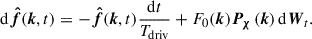 (9)
(9)
Here Tdriv represents the autocorrelation timescale of turbulence, approximately equal to Lbox/(2σ). Where σ is the 3D mass-averaged velocity dispersion computed in the whole simulation. This value divided by the sound speed, cs, is used in the definition of the Mach number, ℳ = σ/cs. Then dt is the integration time step, dWt is a stochastic term following the Wiener process (Schmidt et al. 2009). The power spectrum of turbulent driving is as follows:
 (10)
(10)
The quantity Pχ(k) is the projection operator that balances compressive and solenoidal modes in the Helmholtz decomposition of one mode versus the other,
 (11)
(11)
with P⊥ and P∥ being the perpendicular and parallel projection operators with respect to k (Federrath et al. 2010). The compressive driving fraction χ used here is 0, which corresponds to purely solenoidal turbulence. Finally, the physical force field f(x, t) in the simulations is derived from the Fourier modes:
 (12)
(12)
The coefficient frms serves as a proxy to control the energy injected into the simulations by turbulence. The dependence of ℳ on this coefficient was explored in Brucy et al. 2024 (see their figure 3). Additionally, g(χ) is an empirical corrective factor ensuring that the average power across Fourier modes remains consistent with frms, irrespective of χ.
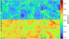 |
Fig. 1. Column density maps for all runs growing in Mach number from left to right and in mean density from top to bottom. This images correspond to the moment when all runs have deposited a similar amount of mass into stellar particles. |
3.4. Self-gravity and star formation
In the second phase of our simulations, we introduced gravity to assess its impact on the SFR. These simulations commence with the density and velocity fields derived from their respective non-gravitational predecessors at 2Tdriv, where Tdriv is the auto-correlation timescale of turbulence, as mentioned in Section 3.3. This approach guarantees that turbulence is fully developed before the activation of gravity.
For the calculation of gravitational potential, we used a multigrid Poisson solver. The process of star formation is monitored through the implementation of sink particles, following methodologies such as those described by Krumholz et al. (2004) and Bleuler & Teyssier (2014). These sink particles are introduced when the gas density surpasses a certain threshold, denoted as ρsink = 3 × 10¹⁰ H cm−3.
Analyses are performed at the time when simulations with equal initial density have accreted the same fraction of the initial gas mass into sink particles: 650 M⊙ (∼2%) in the low-density suite and 140 M⊙ (∼1%) in the high-density suite. These thresholds are reached after one autocorrelation timescale in the low-density runs and one-half an autocorrelation timescale in the high-density runs, where Tdriv = 1.7, 0.49, and 0.17 Myr for ℳ = 1, 3, and 10, respectively. This procedure ensures that each suite is compared at a similar absolute sink mass, capturing the first generation of collapse, while avoiding later phases where unmodelled stellar feedback would become important.
Figure 1 shows projected column density maps for the runs with ⟨ρ⟩ = 103 in the top rows and 104 H/cm3 in the bottom rows. Both figures have the same scale in the colour bar; this way it is evident how the denser runs differ from the lower-density cases. The Mach number changes from left to right in increasing order, as denoted in the bottom part of the lower panels, with ℳ = 1, 3.5, and 10 in the left, centre, and right panels, respectively. As the turbulence increases, the contrast between the box’s densest and lowest-density regions becomes more pronounced. Higher turbulence levels create a higher number of dense filaments and empty pockets between them, while lower turbulence results in smoother gas distributions. The simulations presented here use purely solenoidal turbulence, which likely does not reflect all the conditions in the observed region. Future studies will incorporate mixed turbulence modes. However, it is important to recognise that the lack of compressive turbulence will hinder the formation of dense hubs and ridges, impacting the column density PDF, as suggested by observations. This choice simplified the current study by reducing the number of variables.
Isothermal turbulence is scale-free only in the absence of gravity. Once self-gravity is included, density becomes important since it sets the total mass, which enters the virial ratio. Since the global virial ratio scales as αvir ∝ ℳ2/ρ0, the selected values of Mach number at fixed box size correspond to varying levels of gravitational boundedness. In the present simulations, the virial ratios for the low-density runs are approximately αvir ≈ 7 × 10⁻³, 8.9 × 10⁻², and 0.73 for increasing Mach number; the corresponding values for the high-density runs are roughly an order of magnitude lower. The two densities were chosen to bracket the values inferred in regions targeted by ALMA IMF studies, ensuring observational relevance. Although density is not a fully meaningful control parameter in the scale-free isothermal limit, its use enables a more direct connection to observed systems, which are typically described in terms of density rather than virial ratio.
4. Gas density PDF
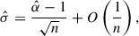
The probability density function (PDF) of gas density in supersonic isothermal flows has been thoroughly examined over time, primarily using numerical simulations. Vazquez-Semadeni (1994) and Nordlund & Padoan (1999) suggested that the gas PDF in these cases follow a lognormal distribution represented as
 (13)
(13)
where δ = ln(ρ/ρ0), ρ0 is the average density, σ0 is the dispersion, δ0 = σ02/2, and
 (14)
(14)
Here ℳ is the Mach number and b is an empirical parameter that could take values of b ≃ 0.5 − 1. A transition in the behaviour of the high-density tail of the gas probability density function (PDF) is observed, characterised by a power-law shape in low-turbulence cases and transitioning to a wider lognormal shape under high turbulence. This evolution remains consistent across varying mean densities. Figures 2 and 3 display the gas PDF in the right panel, accompanied by their respective fits. To quantify and confirm this transition, a fit was applied to the PDFs, evaluated through a χ2-test on a function defined in segments:
 (15)
(15)
 |
Fig. 2. Gas PDF from three simulations with a mean density of ⟨ρ⟩ = 103 H/cm3 (left panel) is depicted. The solid grey lines represent the data, while the dashed lines indicate the fits using Equation (15). The fitted curves are shown in different colours, representing the three turbulence levels: ℳ = 1, 3.5, and 10, displayed in purple, orange, and green, respectively. The circle marker indicates the position of tmin, while the vertical lines mark the start and end of the fit range. The right panel illustrates the relationship between the goodness of fit, measured by the χ2 value, as tmin shifts from the peak to the end of the distribution. |
Here tmin is the transition density above which the PDF behaves as a power law with index β. The fit is conducted with all parameters left free except for tmin, which takes values from the peak of the distribution to the high-density end. This test assesses the significance of employing a dual-function approach–lognormal for low and mid densities and a power law for high densities–against a singular lognormal function for all densities. To fit the composite PDF model in Equation 15, a series of trial transition densities tmin is tested and the value minimising the total χ2 is adopted. For each tmin, the lognormal component fLN(x; σ0, δ0) is fit over x ∈ [xmin, tmin), treating both dispersion σ0 and offset δ0 as free parameters. Continuity at x = tmin is then imposed by setting the power-law amplitude C = fLN(tmin; σ0, δ0), after which only the tail slope β is fit over x ∈ [tmin, xmax]. No additional constraints (e.g. differentiability at tmin or global PDF normalisation) are enforced since our goal is to determine when a pure lognormal suffices and when a power-law tail becomes necessary. This approach contrasts with the more sophisticated normalisation and continuity–differentiability treatment of Khullar et al. (2021), which is beyond the scope of the present study. In the final minimisation, the only free parameters are σ0, δ0, β, and tmin, with C fixed by continuity. The χ2 values, presented in the right panel of Figures 2 and 3, indicate a clear minimum for low-turbulence scenarios. This suggests that transitioning from a lognormal to a power law provides a precise description of the observed density distribution. For high-turbulence scenarios (ℳ = 10), the end of the χ2 curve flattens all the way to the end, signifying that both hypotheses fit the density distributions equally well. However, a singular lognormal description is preferred for its simplicity.
In gravo-turbulent theory, the stellar mass spectrum directly depends on the density PDF. In this context, the final spectrum is sensitive to whether the PDF follows a lognormal function or a power law; the latter predicts a flatter spectrum tail than the former (see Equation 37 and Section 5.4 of Hennebelle & Grudić 2024).
Different functions to describe the IMF–CMF and the scaling of the tail.
Summary table.
5. Cloud mass function and initial mass function
Clouds within the simulations are identified using a version of the HOP clumpfinder (Eisenstein & Hut 1998) called the ecogal wrapper2. While a comprehensive account of the code’s strategy and its results in various simulations appears in Colman et al. (2024), a brief overview is provided here. Initially, the code is provided with a list of cells from an input file, detailing each cell’s position (x, y, z coordinates), mass, and density. A search tree based on cell positions facilitates efficient nearest-neighbour identification. Then the code determines the densest neighbour of each cell, within the default number of neighbours, set to 16, following Eisenstein & Hut (1998) for SPH simulations. This count is deemed optimal for grid simulations, with a minimum of four cells, as per Colman et al. (2024). Increasing the count may yield larger structures, but at the expense of calculation time. A ‘hop’ process traces a chain of densest neighbours to group cells around peak density points, forming a structure now considered a clump, which we use as a proxy for stellar cores in the simulation and will be addressed like that from now on. The procedure also involves boundary analysis to detect cells neighbouring different groups. This is done by defining a saddle density at these boundaries as the average density between adjacent cells from distinct groups. The highest saddle density between group pairs is stored. For grid simulations, eight neighbours are considered to maintain consistency with grid regularity. The Ecogal wrapper from Colman et al. (2024) further evaluates core properties, including size, ellipticity, and internal energies (kinetic, thermal, or gravitational).
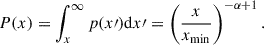
In this analysis, a lower threshold for core identification at 105 H/cm3 is applied, regardless of the mean density of the full box. Alternative thresholds were evaluated, but were deemed unsuitable; lower thresholds identified too many spurious structures as cores, while higher thresholds led to an undersampling of cores. However, even with a density threshold not all detected cores are likely to be collapsing structures that will form stars. As an attempt to minimise the inclusion of non-collapsing gas structure, a CMF is constructed only for cores where the internal thermal energy is less than half of their gravitational energy, Eth < 0.5Egrav, as these will very likely be collapsing cores since gravity dominates. The tail of this constrained CMF and that of the CMF built with the total number of detected cores are shown in Figure 4 for the low-density case and in Figure 5 for the high-density case. This selection criterion focuses on thermal rather than kinetic energy because the calculation of kinetic energy includes infall motions related to gravitational energy, which would incorrectly ignore collapsing cores as dominated by their kinetic energies. The tails of the CCDFs for these CMFs are illustrated in Figures 4 and 5, where the left panels display the total population of detected cores, and the right panels show those meeting the thermal criterion. The solid lines represent the power-law behaviour, with the index α estimated using the MLE method (see Section 2.2). The CCDF of the CMF observed in the W43-MM2&MM3 ridge by ALMA (Pouteau et al. 2022) is depicted as solid black lines including the estimated index. In fitting the CMF and IMF tails, the maximum likelihood requires the finding of a lower bound. For each candidate lower bound xmin, the MLE slope is computed as
 |
Fig. 4. Complementary cumulative distribution function of cores. Shown are the total population of cores (left) and those cores meeting the virial condition Eth < 0.5Ekin (right), for a mean density of ⟨ρ⟩ = 103 H/cm3. The data for the core populations are depicted as solid lines, whereas the estimated slopes for the MLE method are illustrated as dashed lines. The black curves represent observations from ALMA. |
![Mathematical equation: $$ \begin{aligned} \hat{\alpha }= 1 + n\biggl [\sum _{i\,:\,x_i \ge x_{\min }} \ln \frac{x_i}{x_{\min }}\biggr ]^{-1}\!, \end{aligned} $$](/articles/aa/full_html/2026/02/aa53497-24/aa53497-24-eq18.gif) (16)
(16)
and the Kolmogorov–Smirnov statistic D is evaluated between the empirical CDF of the data xi ≥ xmin and the CDF of the fitted power law. The optimal xmin is then chosen as the value minimising D. Uncertainties in  and xmin are estimated via bootstrap resampling using the Python library described in Alstott et al. (2014).
The W43-MM2&MM3 ridge, part of the significant W43 molecular cloud complex, includes two primary components: W43-MM2, the second most massive young protocluster in the ALMA-IMF survey and its less massive neighbour, W43-MM3 (Motte et al. 2022). Together, they form a ridge with a total mass of about 3.5×10⁴ M⊙ spread over approximately 14 pc2 which corresponds to around 2.5 × 10³ M⊙/pc2. This is close to the simulations presented here with mean densities of 104 H/cm3 since the box is of 10 pc per side, meaning that this corresponds to 2.47 × 10³ M⊙/pc2. This ridge is a crucial area of the W43 molecular cloud, located at the intersection of the Scutum-Centaurus spiral arm and the Galactic bar, approximately 5.5 kpc from the Sun. Characterised by its high-density filamentary structures, this region is noted for its efficiency in forming high-mass stars, thus classifying it as a mini-starburst area. The ALMA-IMF consortium reconstructed the CMF in this ridge (Pouteau et al. 2022) and found a flatter power-law index for the distribution tail with a value of 0.95 on the logarithmic formulation. The corresponding CCDF is shown in Figures 4 and 5.
The steepness of the power-law tail of the distribution, indicated by α, correlates with the Mach number of the ISM in these simulations. A steeper mass spectrum of the cores is observed in scenarios with higher turbulence. This pattern holds whether considering the total population or only those meeting the thermal criterion. In the case of Eth < 0.5Egrav, which corresponds more closely with the cores chosen by observers, the scenarios with ℳ = 3.5 and ℳ = 10 yield results that compare well with observations from the W43-MM2&MM3 ridge. The results for the estimation of α for these distributions are summarised in Table 2. Another effect observed here is that, from the total sample to the restricted sample, the CMF tail becomes steeper in low-density cases, whereas the opposite trend is seen in high-density cases.
The IMF generated in the simulations is shown in the left panels of Figures 6 and 7, calculated when each simulation has formed the same mass into stars. The low-mass end of the IMF is shown as grey crosses and is excluded from the present analysis. This is due to the fact that in simulations with an isothermal EOS, both the peak and low-mass tail of the sink mass distribution are resolution-dependent and do not converge, which is a consequence of the scale-free nature of isothermal fragmentation. Increasing the resolution simply shifts the peak to lower masses. In contrast, the high-mass end remains robust across resolutions, motivating the focus on that regime. The central and right panels display the CCDFs of the total stellar populations and the constrained stellar population, respectively. The α estimations in the central panels are done without specifying a value for xmin, while those in the right panels are estimated with xmin = 0.5 M⊙, as the IMF peak is expected to be around this mass. Each curve generated without a fixed xmin starts at the xmin value determined by the automated MLE method. Typically, this value corresponds to the beginning of the final section of the curve that behaves as a power law. A specific xmin condition is applied because the calculation of α can be skewed by the most massive sink particles. This effect is evident in the central panel, where the unconstrained procedure targets only the high-mass tail, which may show power-law behaviour, but does not accurately represent the entire tail. The imposition of a common xmin for all runs is adopted as a complementary approach to the automatic estimation described in Alstott et al. (2014). While the automatic procedure selects xmin by minimising the Kolmogorov–Smirnov distance, and thus accounts for numerical factors such as data completeness, the fixed threshold of xmin = 0.5 M⊙ is introduced as a physically motivated alternative. Other values such as 1 and 2 M⊙ were also tested, and the trend across different Mach numbers was found to be preserved. This choice serves as a case where a common and comparable mass range is considered across all simulations, allowing for a simpler and consistent definition of the high-mass tail in each distribution. Similar to the results of the CMFs tails, an increase in the steepness of the IMF tail is noted with higher turbulence levels. Nonetheless, values of α computed with an imposed xmin of one-half a solar mass fall within the range of the Salpeter value. All the calculated values of α are summarised in Table 2.
 |
Fig. 6. Left panel: IMF for simulations conducted at a lower mean density (⟨ρ⟩ = 103 H/cm3). The dashed and solid lines represent steep (Salpeter) and flatter power law, respectively, for guidance. The part of the IMF that is not used in this analysis is shown in grey. The middle and right panels present the CCDF, normalised to reflect the percentage of sinks with mass exceeding the values on the horizontal axis. The dashed lines in these panels indicate power laws determined by the MLE method. In the middle panel, the MLE method dynamically estimates the value of xmin, while in the right panel, xmin is set at 0.5 M⊙. |
6. Discussions
Figure 8 shows the power-law index, α, of the IMF and CMF tail against the Mach number in simulations. For comparison, the horizontal lines show the Salpeter value (dotted grey) and observation results corresponding to the CMF from the W43-MM2&MM3 ridge (dash-dotted blue) and two IMF from massive clusters 30 Doradus (dash-dot-dotted red) and Arches (dense dash-dotted). Population constraints on stars and cores were tested in the simulations and examined in Section 5; the summary plot in Figure 8 shows the unconstrained results. It is crucial to acknowledge the complexity of star formation physics beyond what is presented here. Not all detected cores may meet the necessary conditions for star formation, and those that do may fragment to form multiple stars. Nonetheless, these findings suggest a connection between the gas PDF, gas core populations, and young stellar populations, consistent with the models proposed by Hennebelle & Chabrier (2008), particularly in high Mach number scenarios where the gas PDF is lognormal and the CMF–IMF tail approaches a Salpeter-like distribution. The idea is that turbulence works against star formation by providing support against gravitational collapse, while also promoting the formation of small structures, thus inducing a steep Salpeter-like tail of the CMF–IMF. It is crucial to recognise that the discussions presented above about turbulence levels, whether high or low, are relevant because all the presented simulations share the same mean density and total mass. It would be more appropriate to focus on whether an environment is dominated by gravity or turbulence. In this context, changes in turbulence levels affect their prominence relative to a common gravitational influence, which remains mostly unchanged between runs. Typically, observed galactic structures are near equipartition or virialisation, otherwise total collapse or evaporation would occur. Therefore, as shown here, the degree to which the pressure ratio favours gravity or turbulence will significantly impact star formation. Notably, Figure 8 illustrates particular examples of top-heavy CMF from the W43+MM2&MM3 ridge and IMF from the Arches cluster near the galactic centre and 30 Doradus in the Large Magellanic Cloud. The considerable mass of these clusters suggests that they are predominantly influenced by gravitational collapse rather than by turbulent support, and thus are similar to the low-turbulence scenarios discussed here.
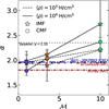 |
Fig. 8. Relation of the power-law index α and the Mach number of the different CMF and IMF extracted from the simulations. The stars correspond to the IMF and the circles to the CMF. The dashed lines connect the results from the low-density cases and the solid lines the high-density cases. The horizontal grey dotted line shows the Salpeter value, the blue dot-dashed line is the index corresponding the CMF measured in W43-MM2&MM3 ridge (Pouteau et al. 2022), the red dot-dot-dashed line corresponds to the index of the IMF tail of 30 Doradus (Schneider et al. 2018), and the red dense dot-dashed line shows the index of the IMF tail of the Arches cluster (Hosek et al. 2019). |
It is important to note that most star formation occurs in clouds with virial ratios αvir ∼ 1–3, consistent with a Salpeter-like IMF (Evans et al. 2022). The top-heavy cases found in the simulations correspond to extremely low virial parameters (αvir ≲ 0.1), such as those arising in the high-density low-Mach set-ups. In reality, such conditions are rare and likely represent extreme environments, for example 30 Doradus or the Arches and Quintuplet clusters.
Direct comparisons with observations are challenging, due to several factors. These simulations are isothermal and scale-independent, whereas the real ISM is neither. On the side of observations, separating velocities from gravitational infall and turbulent gas motions is not trivial. Additionally, while the total mass of young stars in different regions might be similar, the turbulent state of the gas is highly time-dependent and evolves significantly due to feedback. For example, in 30 Doradus and other evolved regions, the gas state reflects the feedback effects and may not correspond to the observed stellar population. As a result, measuring local turbulence directly linked to an IMF is nearly impossible.
One might infer whether a region is gravity-dominated based on its total stellar mass, as massive clusters are more likely to be gravity-dominated. Such a premise is consistent with observations of molecular clouds in the Milky Way, as shown in Figure 17 of Miville-Deschênes et al. (2017), where the virial parameter decreases with increasing cloud mass, suggesting that more massive clouds are gravity-dominated and prone to collapse. A similar scenario is presented in Figure 1 of Kauffmann et al. (2013) for a more complex sample of star-forming regions. Expanding on this rationale, Figure 9 illustrates the distribution of the tail slope of the IMF, α, and cluster stellar mass for a sample of local and distant clusters. While integrating the simulations presented here into this plot would not provide insightful information as the scale-independent nature of an isothermal box would allow us to rescale observables (e.g. the total mass), the simulation results are shown as coloured error bar triangle markers. Nevertherless, Figures 8 and 9 are complementary, and the underlying rationale remains consistent: observations indicate that in gravity-dominated regions mostly top-heavy IMFs (low-α) are observed, whereas simulations suggest that turbulence-dominated environments result in bottom-heavy CMF–IMF (high, Salpeter-like α and above). A key feature of this plot is the absence of data in the high-α and high-stellar-mass quadrant, which further supports the proposed rationale. On the left of Figure 9, i.e the low stellar mass half, clusters consistent with both turbulent-dominated (top half) and gravity-dominated (bottom half) scenarios are present. However, mostly clusters consistent with gravity-dominated scenarios are observed in the high stellar mass half (bottom right quadrant). This trend arises because the turbulent energy required to overcome gravitational collapse in such massive clusters is extremely high, and thus is rarely achieved. To further support this we consider the probability of obtaining an empty upper right quadrant in Figure 9, under the assumption that points are uniformly distributed in the α versus log M plane. Taking as the test area only the rectangular region spanned by the data, the quadrant defined by log(M/M⊙) > 3.1 and α > 2.45 occupies approximately 20.6% of the total area. Assuming uniform sampling over this space, the probability that none of the observed points fall into this quadrant after drawing n samples can be estimated using the formula (1 − f)n, which assumes independent random sampling from a uniform distribution. Here f = 0.206 is the fractional area of the region and n is the number of independent samples. For n = 21 (the number of observed clusters), the probability of observing zero points in this region is approximately 0.78%. Including six additional points from the simulations (total n = 27) reduces this probability to 0.19%3. This simplified calculation illustrates that the absence of data in this region of the plane is unlikely to occur by chance, and is more plausibly explained by physical constraints that limit the formation of high-mass systems with steep IMF slopes.
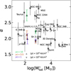 |
Fig. 9. IMF tail power-law index α for the high-mass tail and its relation with the stellar mass of the cluster for the simulations and observations. The horizontal dotted grey line corresponds to the Salpeter value. The values plotted here and their reference can be found in Table A.1. |
This picture suggests that protostellar cores experience reduced efficiency in accumulating mass through gas accretion within highly turbulent high-velocity dispersion environments. Notably, Lee & Hennebelle (2018) analytically predicted that a power-law gas PDF produces a flatter stellar mass spectrum with α ≃ 1.8, in contrast to a lognormal PDF, which results in Salpeter-like values for α, as predicted by Hennebelle & Chabrier (2013). They argue that, in turbulence-dominated cases, a lognormal gas distribution forms; unlike a power-law PDF, this distribution declines too sharply and limits the presence of very dense material, thereby reducing the formation of very massive clumps. This prediction aligns with what is observed in the present simulations. This work presents a direct quantitative test of the Hennebelle & Chabrier (2013) model by establishing a correlation between the slope of the high-density tail of the gas PDF and the high-mass slope of the IMF. While previous studies, such as Nam et al. (2021), have investigated how variations in the velocity power spectrum influence the IMF and have compared the results to the mentioned theory, the present study appears to be the first to explicitly demonstrate such a correlation involving the density PDF slope in simulations. These findings provide new quantitative support for the long-standing idea that the IMF retains memory of the statistical properties of the star-forming gas
7. Conclusions
Simulations of star-forming regions within the interstellar medium (ISM) were conducted at mean densities of 103 H/cm3 and 104 H/cm3. The isothermal nature of these simulations renders them scale-independent or rescalable. At a spatial scale of 10 pc, the resolution achieved is 64 au. These simulations generate individual star particles, or sink particles, which continue to accrete material under specific conditions. Initially, turbulence was injected in uniformly distributed gas until a predetermined turbulence level was reached, after which gravitational collapse was allowed. The level of turbulence, maintained throughout the simulation, was set at three distinct values of ℳ = 1, 3.5, and 10 for each mean density. This set-up facilitated the examination of gas properties and the evolution and interaction between the IMF and CMF as turbulence varies. The primary findings are as follows:
-
Gas PDF is related to turbulence. The PDF of the gas density transitions from a power-law distribution at lower and medium turbulence levels to a lognormal distribution at the highest Mach number tested, irrespective of the mean density.
-
The tail of the mass spectra power law of stars and cores evolves with turbulence. A correlation between the steepness index α of the mass spectrum for cores and stars and the level of turbulence is observed. Scenarios with low turbulence (ℳ = 1 and 3.5) exhibit flatter power-law indexes for the tails of the CMF and IMF, aligning more closely with observations from galactic star-forming regions, as depicted by the dotted line in Figure 8. Conversely, higher-turbulence scenarios demonstrate steeper indexes, aligning more closely with the Salpeter slope. This variation, coupled with the fact that the Salpeter slope value is well out of the estimated error bars for low-turbulence scenarios in the full populations, challenges the universality of the IMF and underscores the potential for its environmental dependence.
-
The CMF and IMF are linked across the tested turbulence range. The evolution of the slope of the distribution tails, across varying turbulence values, consistently aligns between the CMFs and IMFs within the same simulation. This confirms a connection between the two populations.
The present results contribute to addressing several unresolved issues in star formation, such as linking the CMF, IMF, and gas PDF, and mark a step towards understanding these phenomena.
Acknowledgments
The author is grateful to the referee for helping improve the original manuscript and to Juan Soler for fruitful discussion and exchanges. This work has received funding from the French Agence Nationale de la Recherche (ANR) through the project COSMHIC (ANR-20-CE31-0009). NB acknowledges support from the ANR BRIDGES grant (ANR-23-CE31-0005).
References
- Alstott, J., Bullmore, E., & Plenz, D. 2014, PLoS ONE, 9, e85777 [CrossRef] [Google Scholar]
- Alves, J., Lombardi, M., & Lada, C. J. 2007, A&A, 462, L17 [NASA ADS] [CrossRef] [EDP Sciences] [Google Scholar]
- Andersen, M., Zinnecker, H., Moneti, A., et al. 2009, ApJ, 707, 1347 [Google Scholar]
- André, P., Belloche, A., Motte, F., & Peretto, N. 2007, A&A, 472, 519 [NASA ADS] [CrossRef] [EDP Sciences] [Google Scholar]
- André, P., Men’shchikov, A., Bontemps, S., et al. 2010, A&A, 518, L102 [NASA ADS] [CrossRef] [EDP Sciences] [Google Scholar]
- Ascenso, J., Alves, J., Vicente, S., & Lago, M. T. V. T. 2007, A&A, 476, 199 [NASA ADS] [CrossRef] [EDP Sciences] [Google Scholar]
- Ballesteros-Paredes, J., Gazol, A., Kim, J., et al. 2006, ApJ, 637, 384 [Google Scholar]
- Ballesteros-Paredes, J., Hartmann, L. W., Pérez-Goytia, N., & Kuznetsova, A. 2015, MNRAS, 452, 566 [NASA ADS] [CrossRef] [Google Scholar]
- Bate, M. R. 2009, MNRAS, 392, 590 [Google Scholar]
- Bate, M. R., & Bonnell, I. A. 2005, MNRAS, 356, 1201 [Google Scholar]
- Bleuler, A., & Teyssier, R. 2014, MNRAS, 445, 4015 [Google Scholar]
- Brucy, N., Hennebelle, P., Colman, T., & Iteanu, S. 2023, A&A, 675, A144 [NASA ADS] [CrossRef] [EDP Sciences] [Google Scholar]
- Brucy, N., Hennebelle, P., Colman, T., Klessen, R. S., & Le Yhuelic, C. 2024, A&A, 690, A44 [NASA ADS] [CrossRef] [EDP Sciences] [Google Scholar]
- Chabrier, G. 2003, PASP, 115, 763 [Google Scholar]
- Clauset, A., Shalizi, C. R., & Newman, M. E. J. 2009, SIAM Rev., 51, 661 [NASA ADS] [CrossRef] [Google Scholar]
- Colman, T., Brucy, N., Girichidis, P., et al. 2024, A&A, 686, A155 [NASA ADS] [CrossRef] [EDP Sciences] [Google Scholar]
- Cunningham, N., Ginsburg, A., Galván-Madrid, R., et al. 2023, A&A, 678, A194 [NASA ADS] [CrossRef] [EDP Sciences] [Google Scholar]
- Dib, S. 2014, MNRAS, 444, 1957 [NASA ADS] [CrossRef] [Google Scholar]
- Eisenstein, D. J., & Hut, P. 1998, ApJ, 498, 137 [NASA ADS] [CrossRef] [Google Scholar]
- Elmegreen, B. G., & Falgarone, E. 1996, ApJ, 471, 816 [NASA ADS] [CrossRef] [Google Scholar]
- Elmegreen, B. G., & Scalo, J. 2004, ARA&A, 42, 211 [Google Scholar]
- Eswaran, V., & Pope, S. B. 1988, Comput. Fluids, 16, 257 [NASA ADS] [CrossRef] [Google Scholar]
- Federrath, C., Roman-Duval, J., Klessen, R. S., Schmidt, W., & Mac Low, M. M. 2010, A&A, 512, A81 [NASA ADS] [CrossRef] [EDP Sciences] [Google Scholar]
- Galván-Madrid, R., Díaz-González, D. J., Motte, F., et al. 2024, ApJS, 274, 15 [CrossRef] [Google Scholar]
- Guszejnov, D., Grudić, M. Y., Offner, S. S. R., et al. 2022, MNRAS, 515, 4929 [Google Scholar]
- Harayama, Y., Eisenhauer, F., & Martins, F. 2008, ApJ, 675, 1319 [Google Scholar]
- Haugbølle, T., Padoan, P., & Nordlund, Å. 2018, ApJ, 854, 35 [CrossRef] [Google Scholar]
- Hennebelle, P., & Chabrier, G. 2008, ApJ, 684, 395 [Google Scholar]
- Hennebelle, P., & Chabrier, G. 2013, ApJ, 770, 150 [CrossRef] [Google Scholar]
- Hennebelle, P., & Falgarone, E. 2012, A&ARv, 20, 55 [NASA ADS] [CrossRef] [Google Scholar]
- Hennebelle, P., & Grudić, M. Y. 2024, ARA&A, 62, 63 [Google Scholar]
- Hennebelle, P., Brucy, N., & Colman, T. 2024, A&A, 690, A43 [NASA ADS] [CrossRef] [EDP Sciences] [Google Scholar]
- Hopkins, P. F. 2013, MNRAS, 430, 1880 [Google Scholar]
- Hosek, Jr., M. W., Lu, J. R., Anderson, J., et al. 2019, ApJ, 870, 44 [NASA ADS] [CrossRef] [Google Scholar]
- Hur, H., Sung, H., & Bessell, M. S. 2012, AJ, 143, 41 [NASA ADS] [CrossRef] [Google Scholar]
- Hußmann, B., Stolte, A., Brandner, W., Gennaro, M., & Liermann, A. 2012, A&A, 540, A57 [NASA ADS] [CrossRef] [EDP Sciences] [Google Scholar]
- Johnstone, D., Wilson, C. D., Moriarty-Schieven, G., et al. 2000, ApJ, 545, 327 [NASA ADS] [CrossRef] [Google Scholar]
- Kalirai, J. S., Fahlman, G. G., Richer, H. B., & Ventura, P. 2003, AJ, 126, 1402 [NASA ADS] [CrossRef] [Google Scholar]
- Kauffmann, J., Pillai, T., & Goldsmith, P. F. 2013, ApJ, 779, 185 [NASA ADS] [CrossRef] [Google Scholar]
- Könyves, V., André, P., Men’shchikov, A., et al. 2015, A&A, 584, A91 [Google Scholar]
- Kritsuk, A. G., Norman, M. L., & Wagner, R. 2011, ApJ, 727, L20 [NASA ADS] [CrossRef] [Google Scholar]
- Kroupa, P. 2002, Science, 295, 82 [Google Scholar]
- Krumholz, M. R., McKee, C. F., & Klein, R. I. 2004, ApJ, 611, 399 [NASA ADS] [CrossRef] [Google Scholar]
- Lata, S., Pandey, A. K., Kumar, B., et al. 2010, AJ, 139, 378 [Google Scholar]
- Lee, Y.-N., & Hennebelle, P. 2018, A&A, 611, A88 [NASA ADS] [CrossRef] [EDP Sciences] [Google Scholar]
- Li, Y., Klessen, R. S., & Mac Low, M.-M. 2004, Baltic Astron., 13, 377 [Google Scholar]
- Lim, B., Chun, M.-Y., Sung, H., et al. 2013, AJ, 145, 46 [NASA ADS] [CrossRef] [Google Scholar]
- Louvet, F., Hennebelle, P., Men’shchikov, A., et al. 2021, A&A, 653, A157 [NASA ADS] [CrossRef] [EDP Sciences] [Google Scholar]
- Mac Low, M.-M., & Klessen, R. S. 2004, Rev. Mod. Phys., 76, 125 [Google Scholar]
- Mathew, S. S., Federrath, C., & Seta, A. 2023, MNRAS, 518, 5190 [Google Scholar]
- McKee, C. F., & Ostriker, E. C. 2007, ARA&A, 45, 565 [Google Scholar]
- Miville-Deschênes, M.-A., Murray, N., & Lee, E. J. 2017, ApJ, 834, 57 [Google Scholar]
- Moraux, E., Kroupa, P., & Bouvier, J. 2004, A&A, 426, 75 [NASA ADS] [CrossRef] [EDP Sciences] [Google Scholar]
- Motte, F., Andre, P., & Neri, R. 1998, A&A, 336, 150 [NASA ADS] [Google Scholar]
- Motte, F., Bontemps, S., Csengeri, T., et al. 2022, A&A, 662, A8 [NASA ADS] [CrossRef] [EDP Sciences] [Google Scholar]
- Nam, D. G., Federrath, C., & Krumholz, M. R. 2021, MNRAS, 503, 1138 [Google Scholar]
- Nony, T., Motte, F., Louvet, F., et al. 2020, A&A, 636, A38 [NASA ADS] [CrossRef] [EDP Sciences] [Google Scholar]
- Nony, T., Galván-Madrid, R., Brouillet, N., et al. 2024, A&A, 687, A84 [NASA ADS] [CrossRef] [EDP Sciences] [Google Scholar]
- Nordlund, Å. K., & Padoan, P. 1999, in Interstellar Turbulence, eds. J. Franco & A. Carraminana, 218 [Google Scholar]
- Ntormousi, E., & Hennebelle, P. 2019, A&A, 625, A82 [EDP Sciences] [Google Scholar]
- Ostriker, E. C., Gammie, C. F., & Stone, J. M. 1999, ApJ, 513, 259 [NASA ADS] [CrossRef] [Google Scholar]
- Padoan, P., & Nordlund, Å. 2002, ApJ, 576, 870 [NASA ADS] [CrossRef] [Google Scholar]
- Padoan, P., Jones, B. J. T., & Nordlund, Å. P. 1997, ApJ, 474, 730 [NASA ADS] [CrossRef] [Google Scholar]
- Padoan, P., Nordlund, Å., Kritsuk, A. G., Norman, M. L., & Li, P. S. 2007, ApJ, 661, 972 [NASA ADS] [CrossRef] [Google Scholar]
- Pelkonen, V. M., Padoan, P., Haugbølle, T., & Nordlund, Å. 2021, MNRAS, 504, 1219 [NASA ADS] [CrossRef] [Google Scholar]
- Pouteau, Y., Motte, F., Nony, T., et al. 2022, A&A, 664, A26 [NASA ADS] [CrossRef] [EDP Sciences] [Google Scholar]
- Sabbi, E., Sirianni, M., Nota, A., et al. 2008, AJ, 135, 173 [NASA ADS] [CrossRef] [Google Scholar]
- Salpeter, E. E. 1955, ApJ, 121, 161 [Google Scholar]
- Sanhueza, P., Contreras, Y., Wu, B., et al. 2019, ApJ, 886, 102 [Google Scholar]
- Scalo, J. M. 1986, Fund. Cosmic Phys., 11, 1 [NASA ADS] [EDP Sciences] [Google Scholar]
- Scalo, J., Vázquez-Semadeni, E., Chappell, D., & Passot, T. 1998, ApJ, 504, 835 [CrossRef] [Google Scholar]
- Schmidt, W., Hillebrandt, W., & Niemeyer, J. C. 2006, Comput. Fluids, 35, 353 [CrossRef] [Google Scholar]
- Schmidt, W., Federrath, C., Hupp, M., Kern, S., & Niemeyer, J. C. 2009, A&A, 494, 127 [NASA ADS] [CrossRef] [EDP Sciences] [Google Scholar]
- Schneider, F. R. N., Sana, H., Evans, C. J., et al. 2018, Science, 359, 69 [NASA ADS] [CrossRef] [Google Scholar]
- Sharma, S., Pandey, A. K., Ogura, K., et al. 2008, AJ, 135, 1934 [NASA ADS] [CrossRef] [Google Scholar]
- Slesnick, C. L., Hillenbrand, L. A., & Massey, P. 2002, ApJ, 576, 880 [NASA ADS] [CrossRef] [Google Scholar]
- Smith, R. J., Clark, P. C., & Bonnell, I. A. 2009, MNRAS, 396, 830 [Google Scholar]
- Smullen, R. A., Kratter, K. M., Offner, S. S. R., Lee, A. T., & Chen, H. H.-H. 2020, MNRAS, 497, 4517 [Google Scholar]
- Testi, L., & Sargent, A. I. 1998, ApJ, 508, L91 [NASA ADS] [CrossRef] [Google Scholar]
- Teyssier, R. 2002, A&A, 385, 337 [CrossRef] [EDP Sciences] [Google Scholar]
- Tilley, D. A., & Pudritz, R. E. 2004, MNRAS, 353, 769 [Google Scholar]
- Towner, A. P. M., Ginsburg, A., Dell’Ova, P., et al. 2024, ApJ, 960, 48 [NASA ADS] [CrossRef] [Google Scholar]
- Tripathi, A., Pandey, U. S., & Kumar, B. 2014, New Astron., 29, 1 [NASA ADS] [CrossRef] [Google Scholar]
- Vazquez-Semadeni, E. 1994, ApJ, 423, 681 [Google Scholar]
- Wright, N. J., Drew, J. E., & Mohr-Smith, M. 2015, MNRAS, 449, 741 [NASA ADS] [CrossRef] [Google Scholar]
- Yasui, C., Kobayashi, N., Saito, M., Izumi, N., & Ikeda, Y. 2023, ApJ, 943, 137 [NASA ADS] [CrossRef] [Google Scholar]
The index identified in Salpeter (1955) equals 1.35, potentially more recognizable to the reader. Here α is defined as the index in the linear formulation for the sake of consistency in the analyses that follow (see Table 1).
The full version is available in the ecogal_tools GitLab repository, along with test set-ups.
This is a simplified estimate, and it should be noted that the underlying distribution is not uniform and that the dataset is highly heterogeneous.
Appendix A: Mass–size relation
Figure A.1 display the mass–size relation of cores from different simulations and their comparison with various observations. The simulation results align relatively well with observations of the Aquila region in the Gould Belt Könyves et al. (2015), a low star-forming region with a quiescent environment. In contrast, ASHES clumps Sanhueza et al. (2019), associated with high-mass star formation, exhibit higher densities, pressures, and turbulent energies, reflecting an environment that has evolved further due to stellar activity. As a result, these clumps are more massive and do not compare well with the simulations presented here. Additionally, the recovered mass–size relation is fully consistent with the results of Colman et al. (2024), which demonstrated that core mass scales as size3 (black solid line) in simulations across various scales. Here, size is defined as the mean length of the three principal axes of an ellipsoid enclosing all the core’s mass. Runs with low mean density form smaller and less massive halos as turbulence increases. This leads to a higher total number of cores, consequently affecting the uncertainties in the slope derivations of the CMFs computed in section 5.
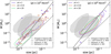 |
Fig. A.1. Mass vs size distribution of the recovered cores from the simulation with a mean density of 103 H/cm3 (left) and ⟨ρ⟩ = 104 H/cm3 (right) are shown in comparison with the core samples of Könyves et al. (2015) (solid grey shaded region) and Sanhueza et al. (2019) (grey hatched region). The contours cover 90% of the recovered cores from the simulations. The dashed line represents the mass–size relation from Elmegreen & Falgarone (1996), and the solid line illustrates the power-law behaviour observed in simulations across different scales by Colman et al. (2024). |
Observation of the high-mass tail of the stellar initial mass function of different stellar cluster and their stellar mass. These values are plotted in figure 9
All Tables
Observation of the high-mass tail of the stellar initial mass function of different stellar cluster and their stellar mass. These values are plotted in figure 9
All Figures
|
Fig. 1. Column density maps for all runs growing in Mach number from left to right and in mean density from top to bottom. This images correspond to the moment when all runs have deposited a similar amount of mass into stellar particles. |
| In the text | |
|
Fig. 2. Gas PDF from three simulations with a mean density of ⟨ρ⟩ = 103 H/cm3 (left panel) is depicted. The solid grey lines represent the data, while the dashed lines indicate the fits using Equation (15). The fitted curves are shown in different colours, representing the three turbulence levels: ℳ = 1, 3.5, and 10, displayed in purple, orange, and green, respectively. The circle marker indicates the position of tmin, while the vertical lines mark the start and end of the fit range. The right panel illustrates the relationship between the goodness of fit, measured by the χ2 value, as tmin shifts from the peak to the end of the distribution. |
| In the text | |
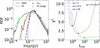 |
Fig. 3. Same as in Fig. 2, but for ⟨ρ⟩ = 104. |
| In the text | |
|
Fig. 4. Complementary cumulative distribution function of cores. Shown are the total population of cores (left) and those cores meeting the virial condition Eth < 0.5Ekin (right), for a mean density of ⟨ρ⟩ = 103 H/cm3. The data for the core populations are depicted as solid lines, whereas the estimated slopes for the MLE method are illustrated as dashed lines. The black curves represent observations from ALMA. |
| In the text | |
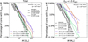 |
Fig. 5. Same as in Fig. 4, but for ⟨ρ⟩ = 104. |
| In the text | |
|
Fig. 6. Left panel: IMF for simulations conducted at a lower mean density (⟨ρ⟩ = 103 H/cm3). The dashed and solid lines represent steep (Salpeter) and flatter power law, respectively, for guidance. The part of the IMF that is not used in this analysis is shown in grey. The middle and right panels present the CCDF, normalised to reflect the percentage of sinks with mass exceeding the values on the horizontal axis. The dashed lines in these panels indicate power laws determined by the MLE method. In the middle panel, the MLE method dynamically estimates the value of xmin, while in the right panel, xmin is set at 0.5 M⊙. |
| In the text | |
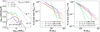 |
Fig. 7. Same as Fig. 6, but for simulations with ⟨ρ⟩ = 104 H/cm3. |
| In the text | |
|
Fig. 8. Relation of the power-law index α and the Mach number of the different CMF and IMF extracted from the simulations. The stars correspond to the IMF and the circles to the CMF. The dashed lines connect the results from the low-density cases and the solid lines the high-density cases. The horizontal grey dotted line shows the Salpeter value, the blue dot-dashed line is the index corresponding the CMF measured in W43-MM2&MM3 ridge (Pouteau et al. 2022), the red dot-dot-dashed line corresponds to the index of the IMF tail of 30 Doradus (Schneider et al. 2018), and the red dense dot-dashed line shows the index of the IMF tail of the Arches cluster (Hosek et al. 2019). |
| In the text | |
|
Fig. 9. IMF tail power-law index α for the high-mass tail and its relation with the stellar mass of the cluster for the simulations and observations. The horizontal dotted grey line corresponds to the Salpeter value. The values plotted here and their reference can be found in Table A.1. |
| In the text | |
|
Fig. A.1. Mass vs size distribution of the recovered cores from the simulation with a mean density of 103 H/cm3 (left) and ⟨ρ⟩ = 104 H/cm3 (right) are shown in comparison with the core samples of Könyves et al. (2015) (solid grey shaded region) and Sanhueza et al. (2019) (grey hatched region). The contours cover 90% of the recovered cores from the simulations. The dashed line represents the mass–size relation from Elmegreen & Falgarone (1996), and the solid line illustrates the power-law behaviour observed in simulations across different scales by Colman et al. (2024). |
| In the text | |
Current usage metrics show cumulative count of Article Views (full-text article views including HTML views, PDF and ePub downloads, according to the available data) and Abstracts Views on Vision4Press platform.
Data correspond to usage on the plateform after 2015. The current usage metrics is available 48-96 hours after online publication and is updated daily on week days.
Initial download of the metrics may take a while.