© The Authors 2026

1. Introduction

The lambda cold dark matter (ΛCDM) model is a well-constrained cosmological model for explaining the expansion of the Universe and for estimating cosmological distances. For the ΛCDM model without radiation and spatial curvature, the Hubble parameter (H) is written as

$$\begin{array}{c}\hfill H(z)=H_0\sqrt{{\mathrm{\Omega }}_{\mathrm{m}}{(1+z)}^3+{\mathrm{\Omega }}_{\mathrm{\Lambda }}},\end{array}$$(1)

where z is the redshift, H₀ is the Hubble constant, Ω_m is the matter density parameter including the baryonic and cold dark matter, and Ω_Λ is the dark energy density parameter related to Ω_Λ ∼ 1 − Ω_m. The cosmological distance is related to z as

$$\begin{array}{c}\hfill D_{\mathrm{L}}=D_{\mathrm{C}}(1+z)=D_{\mathrm{A}}{(1+z)}^2=c(1+z){\displaystyle {\int }_0^z}\frac{\mathrm{d}z\prime }{H(z\prime )},\end{array}$$(2)

where D_L is the luminosity distance, D_C is the comoving distance, and D_A is the angular diameter distance (Hogg 1999). To infer the cosmological parameters H₀, Ω_m, and Ω_Λ, the cosmic distance ladder can be used. This is broadly divided into two categories: the direct distance ladder, and the inverse distance ladder. The direct distance ladder determines the distance from specific celestial objects such as Cepheid variables, Type Ia supernovae (SNe Ia), and the red giant branch (RGB; i.e., tip of the RGB). By fitting Eq. (2) to the distance–redshift relation of the direct distance ladder, the cosmological parameters can be inferred. The inverse distance ladder infers the cosmological parameters by observing early-time processes such as the cosmic microwave background (CMB) and the baryon acoustic oscillation (BAO). The temperature anisotropy observed in the CMB reflects density fluctuations in the early universe. The BAO is an acoustic density wave created by fluctuations in the density of baryonic matter in the plasma state of the early universe. The direct and inverse distance ladders determine the cosmological parameters independently. H₀ as constrained by the two distance ladders differs, however. This is called the Hubble tension. The direct distance ladder constrains H₀ = 73.04 ± 1.04 km/s/Mpc (Riess et al. 2022), and the inverse distance ladder constrains H₀ = 67.4 ± 0.5 km/s/Mpc (Planck Collaboration VI 2020). Solving the Hubble tension currently is a great challenge. One of the tasks for solving the Hubble tension is expanding the local limits of the direct distance ladder because the direct distance ladder clearly has a fatal flaw at higher redshifts. Among the rungs of the direct distance ladder, SNe Ia are known to be the farthest. They reach z = 2.26 (Scolnic et al. 2018). It is difficult to observe distant objects because the intensity dims by (1 + z)³ as a function of z. The direct distance ladder is then accurate to the current and the local universe. Finding new rungs of the ladder with a higher redshift might be a clue to verify whether the locality of the direct distance ladder is the cause of the Hubble tension.

Blazars are a subclass of active galactic nuclei (AGNs) in which relativistic jets powered by a supermassive black hole (SMBH) at the center are observed, being closely aligned to the line of sight. When the relativistic particles in the jet pass through the magnetic field, synchrotron radiation is emitted in a wide range of electromagnetic waves from radio to gamma-rays. Synchrotron radiation is Doppler-boosted by the relativistic effect by δ³ as a function of the Doppler factor δ, and it can therefore be observed from distant blazars at high redshift. In particular, very long baseline interferometry (VLBI) enables us to obtain high-resolution images of the blazars on parsec scales and to measure accurate angular sizes. High-redshift blazars above 6.10 can be imaged by the VLBI (Zhang et al. 2022). Hodgson et al. (2020) applied a method of distance determination using the timescale–size causality to AGN 3C 84, which is not Doppler-boosted (δ ∼ 1). They obtained a consistent distance measurement with SNe Ia and Tully–Fisher measurements. This research has led to the expectation that AGNs might be a direct distance ladder. This method has not yet been applied to a highly Doppler-boosted (δ > 1) source, however. Hodgson et al. (2023) suggested a method of distance determination using Doppler-boosted celestial objects without the Doppler factor. The blazar TXS 0506+056 is classified as an intermediate spectrally peaked BL Lac object AGN (z = 0.3365). On May 13, 2020, the 15 GHz radio flux density reached a maximum of 2.44 Jy and was observed by the Owens Valley Radio Observatory (OVRO) 40 m radio telescope (Hovatta et al. 2021). δ rose to a maximum of 13.6 on June 17, 2017 (Li et al. 2020). We applied the method to TXS 0506+056 to examine whether blazars can be used as a valid means for distance measurements.

In Sect. 2 we derive the angular diameter distance formula of blazars using the variability timescale, flux density, and angular sizes of the emission region. In Sect. 3 we introduce the data and analysis methods we used to obtain the parameters for the distance measurements. In Sect. 4 we describe the analysis results and distance measurements. In Sect. 5 we discuss the results, and in Sect. 6 we conclude.

2. Background

In this section, we describe the method presented by Hodgson et al. (2023) for introducing scaling factors (K, M, and their combination KM³; see below for details), which will also be introduced in Cheong et al. (2025). We used superscripts Q^em, Q^so, and Q^rec over an arbitrary quantity Q, corresponding to the emission, source, and receiver reference frames, respectively. The emission frame is referenced to the relativistic jet of a blazar. The source frame is referenced to the host galaxy of the blazar.

The linear scale (R) of the emission region is constrained by

$$\begin{array}{c}\hfill R_{\nu }^{\mathrm{em}}=gc{\tau }_{\nu }^{\mathrm{em}}=g\frac{c\delta {\tau }_{\nu }^{\mathrm{rec}}}{1+z},\end{array}$$(3)

where ν is the observing frequency, c is the speed of light, τ is a variability timescale, δ is the Doppler factor, and g is a timescale scaling factor (g = 1 for this work). The angular size of the emission region at the receiver frequency ν^rec measured by an observer in the receiver frame, ${\theta }_{R_{\nu }}^{\mathrm{rec}}$, is described as

$$\begin{array}{c}\hfill {\theta }_{R_{\nu }}^{\mathrm{rec}}=\frac{R_{\nu }^{\mathrm{em}}}{D_{\mathrm{A}}}=g\frac{c\delta {\tau }_{\nu }^{\mathrm{rec}}}{(1+z)D_{\mathrm{A}}}·\end{array}$$(4)

The brightness temperature of the emission region $(T_{\mathrm{b}}^{\mathrm{em}})$ is defined in Rayleigh–Jeans regime as

$$\begin{array}{c}\hfill T_{\mathrm{b}}^{\mathrm{em}}=\frac{c^2}{2k_{\mathrm{B}}{({\nu }^{\mathrm{em}})}^2}{I}_{\nu }^{\mathrm{em}},\end{array}$$(5)

where k_B is the Boltzmann constant, and $I_{\nu }^{\mathrm{em}}$ is the intensity of the emission region at the frequency ν^em in the emission frame. The flux density S_ν is written as

$$\begin{array}{c}\hfill S_{\nu }={\displaystyle \int I_{\nu }}(\theta ,\varphi )\mathrm{d}\mathrm{\Omega }=2\pi {\displaystyle {\int }_0^{{\theta }_R}}{I}_{\nu }(\theta )sin\theta \mathrm{d}\theta =K{\theta }_R^2{I}_{\nu }(0),\end{array}$$(6)

where we assumed that I_ν(θ, ϕ) is azimuthally symmetric, θ_R is the angular radius of the brightness distribution of the emission region (with a linear scale of R), and K is a flux-scaling factor corresponding to the intensity distributions (Table 2). The flux density is defined by

$$\begin{array}{c}\hfill S_{\nu }=\frac{h\nu {\mathrm{d}}^{3}n}{\mathrm{d}t\mathrm{d}A\mathrm{d}\nu },\end{array}$$(7)

where n is the number of photons, and h is the Planck constant. The flux density in the emission frame is then obtained by (Boettcher et al. 2012)

$$\begin{array}{c}\hfill S_{\nu }^{\mathrm{em}}=\frac{{\nu }^{\mathrm{em}}}{{\nu }^{\mathrm{rec}}}\frac{\mathrm{d}{t}^{\mathrm{rec}}}{\mathrm{d}{t}^{\mathrm{em}}}\frac{\mathrm{d}{A}^{\mathrm{rec}}}{\mathrm{d}{A}^{\mathrm{em}}}\frac{\mathrm{d}{\nu }^{\mathrm{rec}}}{\mathrm{d}{\nu }^{\mathrm{em}}}{S}_{\nu }^{\mathrm{rec}}=\frac{{(1+z)}^3}{{\delta }^3}{S}_{\nu }^{\mathrm{rec}}.\end{array}$$(8)

Hence, using Eqs. (5), (6), and (8), and Table 1, the brightness temperature in the emission frame can be written as

$$\begin{array}{c}\hfill T_{\mathrm{b}}^{\mathrm{em}}=\frac{c^2}{2k_{\mathrm{B}}{{\nu }^{\mathrm{rec}}}^2}\frac{S_{\nu }^{\mathrm{rec}}}{K{{\theta }_{R_{\nu }}^{\mathrm{rec}}}^2}\frac{1+z}{\delta }·\end{array}$$(9)

Depending on whether the angular size of the emission region is defined using a variability timescale or a VLBI image, the brightness temperature can be divided into a variability brightness temperature and VLBI brightness temperature. The variability brightness temperature in the emission frame ($T_{\mathrm{b},\mathrm{var}}^{\mathrm{em}}$) is defined when ${\theta }_{R_{\nu }}^{\mathrm{rec}}$ is measured by the size–timescale causality (Eq. (4)) as

$$\begin{array}{c}\hfill T_{\mathrm{b},\mathrm{var}}^{\mathrm{em}}=\frac{1}{2k_{\mathrm{B}}{{\nu }^{\mathrm{rec}}}^2}\frac{S_{\nu }^{\mathrm{rec}}{D_{\mathrm{A}}}^2}{K{(g{\tau }_{\nu }^{\mathrm{rec}})}^2}\frac{{(1+z)}^3}{{\delta }^3}·\end{array}$$(10)

The VLBI brightness temperature in the emission frame ($T_{\mathrm{b},\mathrm{VLBI}}^{\mathrm{em}}$) is defined when ${\theta }_{R_{\nu }}^{\mathrm{rec}}=M{\theta }_{\mathrm{FWHM},\nu }$ (Table 2) as

$$\begin{array}{c}\hfill T_{\mathrm{b},\mathrm{VLBI}}^{\mathrm{em}}=\frac{c^2}{2k_{\mathrm{B}}{{\nu }^{\mathrm{rec}}}^2}\frac{S_{\nu }^{\mathrm{rec}}}{K{(M{\theta }_{\mathrm{FWHM},\nu }^{\mathrm{rec}})}^2}\frac{1+z}{\delta },\end{array}$$(11)

where θ_FWHM, ν is the angular full width at half maximum (FWHM) of a circular Gaussian model component in VLBI images, and M is the size scaling factor. We introduce the intrinsic brightness temperature T_b, int which constrains the maximum brightness temperature of AGNs in the emission region. We assumed that $T_{\mathrm{b},\mathrm{var}}^{\mathrm{em}}$ and $T_{\mathrm{b},\mathrm{VLBI}}^{\mathrm{em}}$ are equal to T_b, int. By dividing the cube of Eq. (11) by Eq. (10) and then taking the square root, T_b, int can be expressed as

$$\begin{array}{c}\hfill T_{\mathrm{b},\mathrm{int}}=\sqrt{\frac{{T_{\mathrm{b},\mathrm{VLBI}}^{\mathrm{em}}}^3}{T_{\mathrm{b},\mathrm{var}}^{\mathrm{em}}}}=\frac{c^3}{2k_{\mathrm{B}}{{\nu }^{\mathrm{rec}}}^2}\frac{S_{\nu }^{\mathrm{rec}}g{\tau }_{\nu }^{\mathrm{rec}}}{K{(M{\theta }_{\mathrm{FWHM},\nu }^{\mathrm{rec}})}^3{D}_{\mathrm{A}}}·\end{array}$$(12)

Finally, the angular diameter distance is determined as

$$\begin{array}{c}\hfill D_A=\frac{c^3}{2k_{\mathrm{B}}{T}_{\mathrm{b},\mathrm{int}}{{\nu }^{\mathrm{rec}}}^2}\frac{S_{\nu }^{\mathrm{rec}}g{\tau }_{\nu }^{\mathrm{rec}}}{K{(M{\theta }_{\mathrm{FWHM},\nu }^{\mathrm{rec}})}^3},\end{array}$$(13)

which is a revised form of the formula by Hodgson et al. (2023).

3. Data analysis

To measure the angular sizes of the emission regions and the timescales and peak flux densities of flares, we used 32 epochs of 15 GHz Very Long Baseline Array (VLBA) data from MJD 54838 to MJD 60262 (15 years), which is part of the Monitoring Of Jets in Active galactic nuclei with VLBA Experiments (MOJAVE; Lister et al. 2018). For more precise timescales and peak flux densities, we additionally used 620 epochs of 15 GHz Owens Valley Radio Observatory (OVRO) 40 m single-dish (SD) data from MJD 54474 to MJD 59023 (12 years; Richards et al. 2011), which have a mean cadence of about 7 days (significantly denser than the ∼170-day mean cadence of the VLBA data).

3.1. Circular Gaussian fitting to 15 GHz VLBA data from MOJAVE

To measure the variability timescales and the corresponding angular sizes of the emission region, we fit the 2D circular Gaussian model to the 15 GHz VLBA data using the program DIFMAP (Shepherd et al. 1994), as described in Appendix B. The total results of the Gaussian model fitting are presented in Table B.1. We defined the core component, which is the nearest to the center of images, as C0 and other jet components as J1, J2, and J3 (Fig. 2). We found that the source has a core–jet structure in which the core flux density ranges from 0.221 Jy to 1.906 Jy and the jet flux densities range from 0.073–0.814 Jy. This yields a total model flux density (core and jet flux densities) of 0.294–2.278 Jy. Fig. 1 shows that at the core (VLBA C0), the largest flare peaks on MJD 58834 and the two jet components (VLBA J2 and J3) have a higher flux with a peak on MJD 59433 and MJD 59275, respectively. We also found that the core size changes in the range of 0.048–0.228 mas.

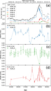Fig. 1. Panel (a): Flux density curves for each VLBA circular Gaussian model component (colored dashed lines), VLBA total clean (dashed black line), and OVRO SD (gray dots). Panels (b), (c), and (d): FWHM curves for VLBA C0, J2, and J3. The VLBA model components are defined by their positions as in Fig. 2.

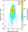Fig. 2. Clean map of TXS 0506+056 on MJD 60126 (July 1, 2023) from MOJAVE overlapped with multiepoch positions of Gaussian model components (VLBA C0, J1, J2, and J3). The major and minor FWHMs of the elliptical clean beam are plotted in the lower left corner. The contours are given at log2 level from three times the root mean square to the peak intensity.

3.2. Flare decomposition of the 15 GHz VLBA model components and OVRO 40 m SD light curves

We decomposed the VLBA light curves using the diffusive nested sampling Python package dnest4 (Brewer & Foreman-Mackey 2018), as described in Appendix C. The results are shown in Fig. 3 and are summarized in Table C.1. In addition, we performed the same decomposition process using the OVRO SD light curve by imposing the decomposition results of the VLBA C0, J2 and J3 as initial parameters. The OVRO data end at MJD 59023, however, while the VLBA data extend to MJD 60262. Therefore, the OVRO SD flux density after MJD 59023 was replaced by the VLBA total clean (VLBA TC) flux density from MJD 59062 to MJD 60262. We named the joint light curve between OVRO SD (MJD 54474–59023) and VLBA TC (MJD 59062–60262) OVRO SD+VLBA+TC.

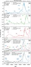Fig. 3. Flare decomposition plots of the VLBA C0 (a), J2 (b), and J3 (c), respectively. For a purpose of comparison, the flare model components in panels (a)–(c) overlap the OVRO SD+VLBA TC light curve in panel (d). A flare decomposition plot (e) of the OVRO SD+VLBA TC light curve using the initial sample shown in panel (d). The solid lines are the single flare model components. The dashed line in each panel describes the sum of all flare model components and the quiescent flux density. All panels note the number of components N, log-likelihood logℒ, χ2, and reduced ${\chi }_d^2$ (d is the degrees of freedom) in the upper left corner. The quiescent flux density (Fqs) is noted in the lower left corner (as well as by the horizontal dotted lines).

4. Results

4.1. Comparison between cross-identified flares

We found that some of the flares decomposed from the VLBA light curves are identified in the OVRO SD+VLBA TC light curve, as noted in Table C.1. We considered the flares from OVRO SD+VLBA TC as cross-identifiers whose parameter estimates (reference time t₀, rising timescale τ, reference flux density F₀, and skewness s) are uniquely identified in the range of their posterior samples from the VLBA light curves, that is, VLBA C0a, C0c, C0d, and C0e (see Fig. 4). The decomposition parameters of the cross-identified flares are compared in Table 3. This comparison shows that the fractional difference of the timescale is |Δτ| = 0.026–0.163 and that of the peak flux density is |ΔF_p| = 0.010–0.223. The fractional offset of distances (D_A) between the cross-identifiers is similar to that of τ × F_p (cf., D_A ∝ τF_p and Eq. (13)), yielding |Δ(τF_p)| = 0.117–0.326. The similarity between the cross-identified flares was also evaluated using the normalized squared Euclidean distance (${\mathrm{NED}}_{\mathit{ij}}^2$), which is defined as in Eq. (14), where Var is the variance, and F_i(t) is the flare model function described in Eq. (C.1),

$$\begin{array}{c}\hfill {\mathrm{NED}}_{\mathit{ij}}^2=0.5\frac{\mathrm{Var}(F_i(t)-F_j(t))}{\mathrm{Var}(F_i(t))+\mathrm{Var}(F_j(t))}·\end{array}$$(14)

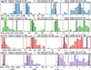Fig. 4. Posterior distributions, point estimates, and credible intervals of the cross-identified flare decomposition parameters t0, τ, F0, and s for flares C0a, C0c, C0d, and C0e (color plots from panels (a) to (d)) and SD4 (C0a), SD14 (C0c), SD19 (C0d), and SD24 (C0e) (gray and black plots from panels (a) to (d)). The bar plots illustrate the posterior distributions. The solid and dashed line plots note the point estimates and interval estimates, respectively.

NED² is equal to zero or far lower than unity for an identical flare, and it approaches unity for significantly different flares. NED² is found to be in the range of 0.0238–0.0804, which is consistent with it being an identical flare.

4.2. Constraining the distance (D_A)

We determined that the flux scaling factor is K = π and the size scaling factor is M = 0.8 (see Table 2). We assumed that the timescale measures the radius perfectly. The timescale scaling factor then is g = 1. We used the equipartition temperature T_eq = 5 × 10¹⁰ K (Readhead 1994) as the intrinsic brightness temperature. We investigated the distance estimates using the core sizes obtained around flares in the period from t₀ − 2τ to t₀ + 2sτ for each flare with its timescale τ and peak flux density F_p, as summarized in Tables D.1 and D.2. The results of the distance measurements are shown in Fig. 5, and their 1σ errors were calculated with the Python package uncertainties. Fig. 5 shows transparent symbols for the distance measurements that deviate by more than 1σ uncertainties from D_A = 948.2 ± 13.5 Mpc, which was calculated with the ΛCDM model, where H₀ = 73.04 ± 1.04 km/s/Mpc and Ω_m = 0.315. When we used the timescale and peak flux density from the VLBA data, all flares of VLBA C0 yield distance estimates that are consistent with the ΛCDM, while those of VLBA J2 and J3 are lower than the ΛCDM distance by 2–4 orders of magnitude. To improve the statistical errors, we also used flares SD4, SD14, SD19, and SD24 from the OVRO SD+VLBA TC data, which were cross-identified with flares C0a, C0c, C0d, and C0e from the VLBA data. Consistent distance measurements were largely obtained using parameters near the flare peak time (see Sect. 5.3 for further discussion).

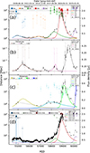Fig. 5. Distance estimates of VLBA C0, J2, J3, and OVRO SD+VLBA TC (from panels (a) to (d)). The solid colored lines show decomposed flares, the colored symbols show the distance estimates using timescales and peak flux densities from the individual flares in corresponding colors, and the black circles show the data (VLBA and OVRO) light curves. The horizontal dashed gray lines note the ΛCDM distance (948.2 ± 13.5 Mpc) with 1σ uncertainty. The color symbols of the distance estimates are opaque when the distance measurements are consistent with the ΛCDM distance within 1σ uncertainties, and they are transparent when the distances are not.

5. Discussions

5.1. Error recognition

The fractional uncertainties of distances for the cross identifiers (C0d/C0e and SD19/SD24) are 40–50% for the VLBA C0 data and 15–26% for the OVRO SD+VLBA TC data. That the uncertainties for OVRO SD+VLBA TC improve by factors of 2–3 is attributed to the fact that the data cadence is about 18.4 times higher and their root mean square error of the flux density is lower by about 3.6 times than that of the VLBA data. The high cadence and precise flux measurements mean that the fractional uncertainties of the distances are smaller by < 5 times for the cross identifiers. The OVRO SD+VLBA TC light curve is the total flux density of the core and all jet components, while the VLBA light curves correspond to individual components. To avoid a potential systematic error from the blending effect of the core and jet components, we decomposed the OVRO SD+VLBA TC light curve as described in Sect. 3.2 and Appendix C. To examine the effect of the systematic error, we compared the parameter offsets (the timescale and peak flux density) between the VLBA and OVRO SD+VLBA TC with the corresponding parameter uncertainties of the VLBA C0 flares (C0a, C0c, C0d, and C0e), as shown in Fig. E.1. We found that the offsets in the flares are within the corresponding parameter uncertainties of VLBA C0.

5.2. Comparison with the standard e-folding timescale

Characteristic timescales of variable emission regions in blazars are determined with various methods, including a log-linear fit (a standard e-folding timescale), a flare decomposition (used in this paper), and a structure function calculation. While the structure function calculation is strongly limited by the data cadence in timescale resolution, the log-linear fit and flare decomposition are free from this limitation. The former two methods are therefore probably largely used to determine the characteristic variability timescale of blazars (e.g., Jorstad et al. 2017; Liodakis et al. 2017). The log-linear fit was used to characterize the variability timescales of resolved jet components (e.g., Jorstad et al. 2017; Hodgson et al. 2020), and the flare decomposition method was largely used to decompose the individual flares in the light curves obtained from single-dish radio observations (e.g., Liodakis et al. 2017, 2018; Kang et al. 2021).

In order to compare the timescales of two methods, we fit a log-linear function to the VLBA C0 light curve for the time period of MJD 57409–58834 (Fig. 6), which yielded an e-folding timescale of about 418 days. We compared this with the decomposition timescales of 178 days (C0c) and 125 days (C0d). The difference of the timescales between the standard e-folding and decomposition cases is most likely attributable to the overlapping multiple flares C0c (peaking on MJD 58230 and reaching F_p = 0.46 Jy) and C0d (peaking on MJD 58850 and reaching F_p = 1.61 Jy). The standard e-folding timescale for the VLBA C0 light curve is similar to the peak-to-peak e-folding timescale for the flares C0c and C0d (about 495 days). Then, the standard e-folding timescale is affected by the flare overlapping and hence overestimated. In order to compare the e-folding timescale of a selected period in individual decomposed flares (e.g., VLBA C0) with the corresponding timescales of a decomposed flare, we investigated the model function and its derivative, as summarized in Appendix F. We found that the e-folding timescale becomes longer than the decomposed timescale, in particular, at the peak of the flare. Therefore, we conclude that the decomposition timescales derived in this study are more robust than the standard e-folding timescales, owing to mitigating the systematic errors of flare overlapping and selecting fitting period.

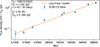Fig. 6. Log-linear fit to the VLBA C0 light curve from MJD 58230 to MJD 58895 and given quiescent flux density Fqs = 0.164 Jy. The fitting function is $S(t)-F_{\mathrm{qs}}=F_{0}exp\left(\frac{t-t_0}{\tau }\right)$. The reference time t0, the reference flux density F0, the standard e-folding timescale τ, χ2, and the quiescent flux density Fqs are noted in the upper right corner.

5.3. Distance determination from blazars

To determine the appropriate angular sizes of the emission regions, we investigated the systematics of the angular sizes on the distance estimates. We calculated the weighted mean distance using the timescales and peak flux densities of each flare (C0a, C0b, C0c, C0d, C0e, J2a, J2b, J2c, J3a, J3b, J3c, and J3d) and the angular sizes of the corresponding individual components (VLBA C0, J2, and J3) obtained in the time from t₀ − aτ to t₀ + asτ, as described in Fig. 7. As the time range of averaging distances increases (i.e., a increases), the weighted mean distance largely decreases (i.e., a larger offset to the ΛCDM distance, except for C0e and SD24), although the corresponding scatter uncertainty decreases. To determine accurate distances, we chose angular sizes near flare peaks. All of the cross-identified flares SD4 (C0a), SD14 (C0c), SD19 (C0d), and SD24 (C0e) yielded consistent distance measurements using the accurate timescales and peak flux densities from the high-cadence SD light curve. The C0b flare was not cross-identified with any of the SD flares, and it therefore yielded inaccurate distance measurements. Additionally, we found that the largest flare SD19 (C0d) enabled us to obtain the most precise and accurate distance of the source.

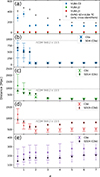Fig. 7. Weighted mean of distances. The distances were calculated using the timescales and peak flux densities of each flare (C0a, C0b, C0c, C0d, C0e, J2a, J2b, J2c, J3a, J3b, J3c, and J3d) and the angular sizes of the corresponding individual components (VLBA C0, J2, and J3) obtained in the time from t0 − aτ to t0 + asτ. Panel (a) shows the weighted means of all distances estimated for VLBA C0 (blue circles), J2 (green circles), J3 (red circles), and OVRO SD+VLBA TC (gray circles). The other panels (b)–(e) show the weighted mean distances of C0a (blue squares), C0c (green pentagons), C0d (red stars), and C0e (purple crosses), respectively, with the weighted mean distances for the corresponding cross-identifiers (black outlined symbols). The horizontal dashed gray lines show the ΛCDM distance (948.2 ± 13.5 Mpc) with the 1σ uncertainty.

5.4. Unresolvable components

In a Gaussian fitting, we were unable to obtain a solution that converged to only one for each epoch because of the unresolvable but apparently significant components near the core. In the period of MJD 54838–58468, the reduced χ² of the best-fitting Gaussian models was improved to 1.071–1.636. From MJD 58699 to MJD 59207, however, the reduced χ² of the best-fitting Gaussian model increased to 5.734–9.546. The errors of the core flux densities and FWHM are therefore larger because of the high σ_rms (Eq. (B.2)). When unresolvable components are added near the core, the χ² might be improved to about 1–2. Because the unresolvable component does not appear continuously in the fitting, however, the flux of the core looks as if it fluctuated. This prevents us from determining an accurate timescale and flux density variation in VLBA C0. If the VLBI observation had a high resolution and dynamic range, they would be resolvable.

6. Conclusions

We measured the distances of blazar TXS 0506+056 using the variability timescale, the flare peak flux density, and the angular sizes of the core and jets, and we assumed an equipartition brightness temperature. The variability timescale and the flare peak flux density were obtained from the 15 GHz VLBA and OVRO SD+VLBA TC light curves. The core sizes were measured using the 15 GHz VLBA data. We summarize our findings below.

1. We obtained distance measurements consistent with the ΛCDM model within a 1σ uncertainty when the core sizes were measured in the period of t₀ − 2τ to t₀ + 2sτ, which includes the flare peaks for each flare. This implies that the optimal angular size of the flaring core is well determined near the flare peak for measuring a consistent distance.

2. We also emphasize that the distance estimates are underestimated when the angular sizes of the jet components are used in any time period. This implies that the distance estimations seem to work well for the core component, probably because the angular sizes of the core are properly measured, whereas those of jet are overestimated. It is necessary to investigate this issue further in future studies.

3. The high cadence and small errors of the OVRO data meant that the combined data of OVRO SD and VLBA TC data enabled a far preciser estimation than the VLBA C0 data.

4. After avoiding a potential systematic error from the blending effect of the core and jet components with the OVRO SD+VLBA TC light-curve decomposition, we found that the offsets in the flares are within the corresponding parameter uncertainties of VLBA C0.

5. One of the dominant factors affecting the distance measurements is θ_FWHM because the distance depends on ${\theta }_{\mathrm{FWHM}}^{-3}$, whose uncertainty is as large as 40% for VLBA C0.

6. We found that the decomposed timescale enabled us to obtain distances that were consistent with the ΛCDM. We strongly suggest to decompose the light curves when the variability timescales are to be obtained properly.

7. In a circular Gaussian fitting, we decided to fit only resolvable components. From MJD 58699 to MJD 59207, we were only able to improve the χ² in a range of 5.734–9.546, however, except for unresolvable components. When more high-resolution VLBI observations over a wider dynamic range are available, preciser model parameters will be obtained, such as θ_FWHM, and the uncertainty of distance measurement can be decreased.

8. We suggest that the best distance of the source is ${941}_{-64}^{+59}$ Mpc, that is, the weighted mean of distances from t₀ − 0.5τ to t₀ + 0.5sτ of the largest OVRO SD flare (SD19). This is comparable to the ΛCDM distance of 948.2 ± 13.5 Mpc. The results were obtained under the assumption of a disk brightness morphology, an equipartition brightness temperature (T_b, int = 5 × 10¹⁰ K), and a perfect radius (g = 1).

Acknowledgments

This work was supported by the National Research Foundation of Korea (NRF) grant funded by the Korea government (MSIT) (2020R1A2C2009003, RS-2025-00562700). This research has made use of data from the MOJAVE database that is maintained by the MOJAVE team (Lister et al. 2018). This research has made use of data from the OVRO 40-m monitoring program (Richards et al. 2011), supported by private funding from the California Institute of Technology and the Max Planck Institute for Radio Astronomy, and by NASA grants NNX08AW31G, NNX11A043G, and NNX14AQ89G and NSF grants AST-0808050 and AST-1109911. Uncertainties: a Python package for calculations with uncertainties, Eric O. LEBIGOT, http://pythonhosted.org/uncertainties/.

References

Appendix A: Size and flux scaling along projected brightness morphologies

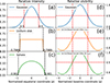Fig. A.1. Theoretical visibility distributions (right panels from (d) to (f)) corresponding to intensity distributions (left penels from (a) to (c)). Red dashed lines denote FWHM and black dashed lines denote radius. Blue (panels (a) and (d)), orange (panels (b) and (e)), and green (panels (c) and (f)) solid lines mean Gaussian, uniform disk, and sphere intensity distributions, respectively. All visibility distributions show the same FWHMs.

Suppose that the projected brightness morphology of the emission region is elliptic cylindrical symmetric. The intensities of example morphologies are shown in Table A.1. p is the normalized coordinate defined as

$$\begin{array}{c}\hfill p\equiv \frac{1}{{\theta }_R}\sqrt{\frac{l^2}{a^2}+m^2}=\frac{r}{{\theta }_R}\sqrt{\frac{{sin}^2\varphi }{a^2}+{cos}^2\varphi },\end{array}$$(A.1)

where (l, m) is the equatorial coordinate system, and (r, ϕ) is the corresponding polar coordinate system. a is the ratio of the minor to major axes (0 < a ≤ 1). θ_R is the radius of major axis for finite morphologies such as disk, ellipsoid, and cone. θ_R is the s-σ boundary of major axis for a Gaussian morphology whose size is infinite. When $s=\sqrt{2ln2}$ for a Gaussian morphology, θ_R = θ_FWHM/2. I₀ is the center intensity, where p = 0. The flux density (S) of morphologies is calculated as

$$\begin{array}{cc}\hfill S& ={\displaystyle {\int }_0^{2\pi }}{\displaystyle {\int }_0^{\infty }}I(r,\varphi )r\mathrm{d}r\mathrm{d}\varphi \hfill \\ \hfill & ={\displaystyle {\int }_0^{2\pi }}{\displaystyle {\int }_0^{\infty }}{\theta }_R^2(\frac{{sin}^2\varphi }{a^2}+{cos}^2\varphi {)}^{-1}I(p)p\mathrm{d}p\mathrm{d}\varphi \hfill \\ \hfill & ={\theta }_R^2{\displaystyle {\int }_0^{2\pi }}(\frac{{sin}^2\varphi }{a^2}+{cos}^2\varphi {)}^{-1}\mathrm{d}\varphi {\displaystyle {\int }_0^{\infty }}I(p)p\mathrm{d}p\hfill \\ \hfill & =2\pi a{\theta }_R^2{\displaystyle {\int }_0^{\infty }}I(p)p\mathrm{d}p=Ka{\theta }_R^2{I}_0,\hfill \end{array}$$(A.2)

where the flux scaling factor K is defined as

$$\begin{array}{c}\hfill K\equiv \frac{2\pi }{I_0}{\displaystyle {\int }_0^{\infty }}I(p)p\mathrm{d}p.\end{array}$$(A.3)

Visibility is Fourier transformation of the intensity, and the visibility functions of the intensity distributions in Table A.1 are shown in Table A.2.

q is the normalized coordinate defined as

$$\begin{array}{c}\hfill q\equiv 2\pi {\theta }_R\sqrt{a^2{u}^2+v^2}=2\pi {\theta }_R\rho \sqrt{a^2{sin}^2\lambda +{cos}^2\lambda },\end{array}$$(A.4)

where (u, v) is the baseline coordinate system, and (ρ, λ) is the corresponding polar coordinate system. It is assumed that the horizontal cross section bounded by the FWHM of the visibility functions will be the same between finite morphologies and a Gaussian morphology. The ellipse equation of the finite morphology cross section bounded by the FWHM is

$$\begin{array}{c}\hfill q_{1/2}=2\pi {\theta }_R\rho \sqrt{a^2{sin}^2\lambda +{cos}^2\lambda },\end{array}$$(A.5)

where q_1/2 = V⁻¹(V(0)/2), and V⁻¹ is the inverse function of V. For the Gaussian morphology, $q_{1/2}=s\sqrt{2ln2}$. When θ_R = θ_FWHM/2, q_1/2 = 2ln2. Then, the ellipse equation of the Gaussian morphology cross section bounded by the FWHM is

$$\begin{array}{c}\hfill 2ln2=\pi {\theta }_{\mathrm{FWHM}}\rho \sqrt{a^2{sin}^2\lambda +{cos}^2\lambda }.\end{array}$$(A.6)

Under the assumption that the horizontal cross section bounded by the FWHM of the visibility functions is the same between finite morphologies and a Gaussian morphology, Eq. (A.5) is equal to Eq. (A.6), yielding

$$\begin{array}{c}\hfill {\theta }_R=\frac{q_{1/2}}{4ln2}{\theta }_{\mathrm{FWHM}}=M{\theta }_{\mathrm{FWHM}},\end{array}$$(A.7)

where the size scaling factor M is defined as

$$\begin{array}{c}\hfill M\equiv \frac{q_{1/2}}{4ln2}.\end{array}$$(A.8)

Appendix B: Circular Gaussian fitting to 15 GHz VLBA data from MOJAVE

In this section we describe the 2D circular Gaussian model fitting with the 15 GHz VLBA data. The cell size of VLBI maps was set to 0.1 × 0.1 mas² with 1024 × 1024 pixels, and a natural weighting is imposed. We performed the model fitting with an increasing number of model components (M). We stopped the fitting when the reduced χ² improvement was less than 10 %:

$$\begin{array}{c}\hfill \frac{1}{m}\frac{{\chi }_{\mathrm{vis}}^2(M-m)-{\chi }_{\mathrm{vis}}^2(M)}{{\chi }_{\mathrm{vis}}^2(M-m)}<0.1,\end{array}$$(B.1)

where ${\chi }_{\mathrm{vis}}^2(M)$ is the visibility reduced χ² with respect to the number of model components M, and m is the number of additional components. The best fitting Gaussian model components were obtained only when the angular sizes FWHM (θ_FWHM) were larger than the minimum resolvable angular sizes even if the addition of another model component satisfied the reduced χ² criteria. The approximated 1σ errors σ_peak, σ_tot, and σ_FWHM corresponding to S_peak, S_tot, and θ_FWHM, respectively, are determined by

$$\begin{array}{c}\hfill {\sigma }_{\mathrm{peak}}={\sigma }_{\mathrm{rms}}(1+\frac{S_{\mathrm{peak}}}{{\sigma }_{\mathrm{rms}}}{)}^{1/2},{\sigma }_{\mathrm{tot}}={\sigma }_{\mathrm{peak}}(1+\frac{S_{\mathrm{tot}}^2}{S_{\mathrm{peak}}^2}{)}^{1/2},{\sigma }_{\mathrm{FWHM}}={\theta }_{\mathrm{FWHM}}\frac{{\sigma }_{\mathrm{peak}}}{S_{\mathrm{peak}}},\end{array}$$(B.2)

where S_peak, S_tot, and σ_rms are the peak flux density, the total flux density, and the root-mean-square (RMS) of the model component, respectively. We determined that the σ_rms calculation region is the combined area of the model component and the clean beam area constrained by the FWHM. The minimum resolvable angular size θ_min of a Gaussian component in a natural-weighting image is determined, following Lobanov (2005), as

$$\begin{array}{c}\hfill {\theta }_{\min }=\frac{4}{\pi }[\pi {{\theta }_{\mathrm{FWHM}}}^{2}ln2ln(\frac{\mathrm{S}/\mathrm{N}}{\mathrm{S}/\mathrm{N}-1}){]}^{1/2},\end{array}$$(B.3)

where the signal-to-noise ratio (S/N) is defined by S/N = S_peak/σ_rms.

Appendix C: Flare decomposition

The total number of decomposed flares is determined by trans-dimensional Bayesian inference (Brewer 2014). Let S[k] be the observed flux density of light curves and σ_S[k] the 1σ error at k^th epoch. We assume that a light curve consists of exponential flares as follows (Kang et al. 2021)

$$\begin{array}{c}\hfill F_i(t)=2F_{0,i}[exp(\frac{t_{0,i}-t}{{\tau }_i})+exp(\frac{t-t_{0,i}}{s_i{\tau }_i}){]}^{-1}.\end{array}$$(C.1)

Each flare has four parameters, the reference time t_0, i, the reference flux density F_0, i = F_i(t_0, i), the rising timescale τ_i, and the skewness s_i, which is the ratio of decaying to rising timescale for the i^th flare. The multi-flare model is constructed as

$$\begin{array}{c}\hfill F(t)={\displaystyle \sum _{i=1}^N}{F}_i(t)+F_{\mathrm{qs}},\end{array}$$(C.2)

where N is the number of flares and F_qs is the quiescent flux density. The peak time t_p, i and the peak flux density F_p, i of each flare are derived by the local maxima of Eq. (C.1) as

$$\begin{array}{c}\hfill t_{\mathrm{p},i}=t_{0,i}+\frac{s_i\tau }{s_i+1}ln{s}_i,\end{array}$$(C.3)

$$\begin{array}{c}\hfill F_{\mathrm{p},i}=2F_{0,i}[s_i^{-s_i/(s_i+1)}+s_i^{1/(s_i+1)}{]}^{-1}.\end{array}$$(C.4)

We introduced hyper parameters that describe prior distributions of the flare parameters (Brewer 2014). μ_F0, μ_τ, and μ_s are means of prior distributions for F_0, i, τ_i, and s_i, and σ_s is the half width of a uniform prior distribution for s_i. The likelihood ℒ is derived from the joint independent normal distribution as

$$\begin{array}{c}\hfill \mathcal{L}={(2\pi )}^{-\frac{K}{2}}{\displaystyle \prod _{k=1}^K}\frac{1}{{\sigma }_S[k]}exp[-\frac{1}{2}(\frac{S[k]-F(t[k])}{{\sigma }_S[k]}{)}^2],\end{array}$$(C.5)

where t[k] is a date of k^th epoch, and K is the total number of epochs. We chose the maximum likelihood sample in posterior samples as a point estimation. We estimated the Gaussian kernel density of posterior samples using the Python library scikit-learn (Pedregosa et al. 2011) to estimate the 1σ Bayesian credible interval considered as the 1σ error of parameters. When posterior samples include several numbers of components N, we selected the minimum reduced χ² result. We calculate the 1σ error of t_p, i and F_p, i by using the Python package uncertainties.

Appendix D: Distance measurements using all VLBA and OVRO SD+VLBA TC flares in all VLBA epochs

We summarized the distance estimates using all VLBA and OVRO SD+VLBA TC flares in all VLBA epochs in Tables D.1 and D.2.

Appendix E: Parameter uncertainties and offsets

To investigate the effect of the systematic error from the OVRO SD+VLBA TC on estimating the model parameters of the flare decomposition (Table C.1) and the distances, we compared the parameter offsets (the timescale and peak flux density) between VLBA and OVRO SD+VLBA TC with the corresponding parameter uncertainties of VLBA C0 flares (C0a, C0c, C0d, and C0e) as shown in Fig. E.1. The fractional offsets (cross symbols) of the parameters (τ, F_p, and τ × F_p) overlap with the fractional errors (open boxes) from VLBA. We found that the offsets in the flares are within the corresponding parameter uncertainties of VLBA C0.

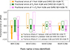Fig. E.1. Fractional errors and offsets of decomposition parameters (timescales in orange, peak flux densities in green, and their multiplications in pink). Fractional errors are plotted as open boxes for VLBA and filled boxes for OVRO SD+VLBA TC, and fractional offsets are cross symbols.

Appendix F: The difference between standard e-folding timescales and decomposition timescales

In order to compare the e-folding timescale of a selected period in individual decomposed flare (e.g., VLBA C0) with the corresponding timescales of decomposed flare, we investigated the derivatives (∂lnF(t)/∂t) of a simulated flare Eq. (C.1).

$$\begin{array}{c}\hfill \frac{\partial lnF(t)}{\partial t}=-\frac{1}{\tau }\frac{-exp(\frac{t_0-t}{\tau })+\frac{1}{s}exp(\frac{t_0-t}{s\tau })}{exp(\frac{t_0-t}{\tau })+exp(\frac{t_0-t}{s\tau })}\end{array}$$(F.1)

As a result, we found that the derivative (Eq. (F.1)) changes as a function of time with approaching 1/τ (t ≪ t₀) and −1/sτ (t ≫ t₀) and converging to zero at the peak of the flare, implying that the e-folding timescale (similar to the inverse derivative (∂lnF(t)/∂t)⁻¹) becomes larger than the decomposed timescale (τ) in particular at the near the peak of the flare. Therefore, flares should always be decomposed.

All Tables

All Figures

	Fig. 1. Panel (a): Flux density curves for each VLBA circular Gaussian model component (colored dashed lines), VLBA total clean (dashed black line), and OVRO SD (gray dots). Panels (b), (c), and (d): FWHM curves for VLBA C0, J2, and J3. The VLBA model components are defined by their positions as in Fig. 2.
In the text

	Fig. 2. Clean map of TXS 0506+056 on MJD 60126 (July 1, 2023) from MOJAVE overlapped with multiepoch positions of Gaussian model components (VLBA C0, J1, J2, and J3). The major and minor FWHMs of the elliptical clean beam are plotted in the lower left corner. The contours are given at log2 level from three times the root mean square to the peak intensity.
In the text

Fig. 3. Flare decomposition plots of the VLBA C0 (a), J2 (b), and J3 (c), respectively. For a purpose of comparison, the flare model components in panels (a)–(c) overlap the OVRO SD+VLBA TC light curve in panel (d). A flare decomposition plot (e) of the OVRO SD+VLBA TC light curve using the initial sample shown in panel (d). The solid lines are the single flare model components. The dashed line in each panel describes the sum of all flare model components and the quiescent flux density. All panels note the number of components N, log-likelihood logℒ, χ2, and reduced ${\chi }_d^2$ (d is the degrees of freedom) in the upper left corner. The quiescent flux density (Fqs) is noted in the lower left corner (as well as by the horizontal dotted lines).

In the text

Fig. 4. Posterior distributions, point estimates, and credible intervals of the cross-identified flare decomposition parameters t0, τ, F0, and s for flares C0a, C0c, C0d, and C0e (color plots from panels (a) to (d)) and SD4 (C0a), SD14 (C0c), SD19 (C0d), and SD24 (C0e) (gray and black plots from panels (a) to (d)). The bar plots illustrate the posterior distributions. The solid and dashed line plots note the point estimates and interval estimates, respectively.

In the text

Fig. 5. Distance estimates of VLBA C0, J2, J3, and OVRO SD+VLBA TC (from panels (a) to (d)). The solid colored lines show decomposed flares, the colored symbols show the distance estimates using timescales and peak flux densities from the individual flares in corresponding colors, and the black circles show the data (VLBA and OVRO) light curves. The horizontal dashed gray lines note the ΛCDM distance (948.2 ± 13.5 Mpc) with 1σ uncertainty. The color symbols of the distance estimates are opaque when the distance measurements are consistent with the ΛCDM distance within 1σ uncertainties, and they are transparent when the distances are not.

In the text

	Fig. 6. Log-linear fit to the VLBA C0 light curve from MJD 58230 to MJD 58895 and given quiescent flux density Fqs = 0.164 Jy. The fitting function is $S(t)-F_{\mathrm{qs}}=F_{0}exp\left(\frac{t-t_0}{\tau }\right)$. The reference time t0, the reference flux density F0, the standard e-folding timescale τ, χ2, and the quiescent flux density Fqs are noted in the upper right corner.
In the text

Fig. 7. Weighted mean of distances. The distances were calculated using the timescales and peak flux densities of each flare (C0a, C0b, C0c, C0d, C0e, J2a, J2b, J2c, J3a, J3b, J3c, and J3d) and the angular sizes of the corresponding individual components (VLBA C0, J2, and J3) obtained in the time from t0 − aτ to t0 + asτ. Panel (a) shows the weighted means of all distances estimated for VLBA C0 (blue circles), J2 (green circles), J3 (red circles), and OVRO SD+VLBA TC (gray circles). The other panels (b)–(e) show the weighted mean distances of C0a (blue squares), C0c (green pentagons), C0d (red stars), and C0e (purple crosses), respectively, with the weighted mean distances for the corresponding cross-identifiers (black outlined symbols). The horizontal dashed gray lines show the ΛCDM distance (948.2 ± 13.5 Mpc) with the 1σ uncertainty.

In the text

Fig. A.1. Theoretical visibility distributions (right panels from (d) to (f)) corresponding to intensity distributions (left penels from (a) to (c)). Red dashed lines denote FWHM and black dashed lines denote radius. Blue (panels (a) and (d)), orange (panels (b) and (e)), and green (panels (c) and (f)) solid lines mean Gaussian, uniform disk, and sphere intensity distributions, respectively. All visibility distributions show the same FWHMs.

In the text

	Fig. E.1. Fractional errors and offsets of decomposition parameters (timescales in orange, peak flux densities in green, and their multiplications in pink). Fractional errors are plotted as open boxes for VLBA and filled boxes for OVRO SD+VLBA TC, and fractional offsets are cross symbols.
In the text

References

- Boettcher, M., Harris, D. E., & Krawczynski, H. 2012, Relativistic Jets from Active Galactic Nuclei (Wiley) [Google Scholar]
- Brewer, B. J. 2014, arXiv e-prints [arXiv:1411.3921] [Google Scholar]
- Brewer, B. J., & Foreman-Mackey, D. 2018, J. Stat. Softw., 86, 1 [CrossRef] [Google Scholar]
- Cheong, W. Y., Lee, S.-S., Song, C., et al. 2025, A&A, 703, L6 [NASA ADS] [CrossRef] [EDP Sciences] [Google Scholar]
- Hodgson, J. A., L’Huillier, B., Liodakis, I., Lee, S.-S., & Shafieloo, A. 2020, MNRAS, 495, L27 [Google Scholar]
- Hodgson, J. A., L’Huillier, B., Liodakis, I., Lee, S.-S., & Shafieloo, A. 2023, MNRAS, 521, L44 [Google Scholar]
- Hogg, D. W. 1999, arXiv e-prints [astro-ph/9905116] [Google Scholar]
- Hovatta, T., Lindfors, E., Kiehlmann, S., et al. 2021, A&A, 650, A83 [NASA ADS] [CrossRef] [EDP Sciences] [Google Scholar]
- Jorstad, S. G., Marscher, A. P., Morozova, D. A., et al. 2017, ApJ, 846, 98 [Google Scholar]
- Kang, S., Lee, S. S., Hodgson, J., et al. 2021, A&A, 651, A74 [NASA ADS] [CrossRef] [EDP Sciences] [Google Scholar]
- Li, X., An, T., Mohan, P., & Giroletti, M. 2020, ApJ, 896, 63 [NASA ADS] [CrossRef] [Google Scholar]
- Liodakis, I., Marchili, N., Angelakis, E., et al. 2017, MNRAS, 466, 4625 [NASA ADS] [CrossRef] [Google Scholar]
- Liodakis, I., Hovatta, T., Huppenkothen, D., et al. 2018, ApJ, 866, 137 [Google Scholar]
- Lister, M. L., Aller, M. F., Aller, H. D., et al. 2018, ApJS, 234, 12 [CrossRef] [Google Scholar]
- Lobanov, A. P. 2005, arXiv e-prints [astro-ph/0503225] [Google Scholar]
- Pedregosa, F., Varoquaux, G., Gramfort, A., et al. 2011, J. Mach. Learn. Res., 12, 2825 [Google Scholar]
- Planck Collaboration VI. 2020, A&A, 641, A6 [NASA ADS] [CrossRef] [EDP Sciences] [Google Scholar]
- Readhead, A. C. S. 1994, ApJ, 426, 51 [Google Scholar]
- Richards, J. L., Max-Moerbeck, W., Pavlidou, V., et al. 2011, ApJS, 194, 29 [Google Scholar]
- Riess, A. G., Yuan, W., Macri, L. M., et al. 2022, ApJ, 934, L7 [NASA ADS] [CrossRef] [Google Scholar]
- Scolnic, D. M., Jones, D. O., Rest, A., et al. 2018, ApJ, 859, 101 [NASA ADS] [CrossRef] [Google Scholar]
- Shepherd, M. C., Pearson, T. J., & Taylor, G. B. 1994, BAAS, 26, 987 [NASA ADS] [Google Scholar]
- Zhang, Y., An, T., Frey, S., Gabányi, K. É., & Sotnikova, Y. 2022, ApJ, 937, 19 [NASA ADS] [CrossRef] [Google Scholar]