| Issue |
A&A
Volume 706, February 2026
|
|
|---|---|---|
| Article Number | A164 | |
| Number of page(s) | 22 | |
| Section | Extragalactic astronomy | |
| DOI | https://doi.org/10.1051/0004-6361/202554969 | |
| Published online | 10 February 2026 | |
Emission-line and continuum reverberation mapping of the NLS1 galaxy WPVS 48
1
Institut für Astrophysik und Geophysik, Universität Göttingen Friedrich-Hund-Platz 1 37077 Göttingen, Germany
2
Department of Physics, Faculty of Natural Sciences, University of Haifa Haifa 3498838, Israel
3
Haifa Research Center for Theoretical Physics and Astrophysics, University of Haifa Haifa 3498838, Israel
4
Ruhr University Bochum, Faculty of Physics and Astronomy, Astronomical Institute (AIRUB) 44780 Bochum, Germany
5
School of Physics & Astronomy and the Wise Observatory, Tel-Aviv University Tel-Aviv 6997801, Israel
★ Corresponding author: This email address is being protected from spambots. You need JavaScript enabled to view it.
Received:
1
April
2025
Accepted:
8
November
2025
Abstract
Context. WPVS 48 is a nearby narrow-line Seyfert 1 galaxy without previous analysis of the broad-line region (BLR) by means of optical spectroscopic reverberation mapping.
Aims. By studying the continuum and emission line variability of WPVS 48, our aim was to infer the BLR size as well as the mass of the central supermassive black hole (SMBH).
Methods. We analysed data from a dedicated optical spectroscopic reverberation mapping campaign of WPVS 48 taken with the 10 m Southern African Large Telescope (SALT) at 24 epochs over a period of seven months between December 2013 and June 2014.
Results. WPVS 48 shows variability throughout the campaign. We find a stratified BLR, where the variability amplitude of the integrated emission lines decreases with distance to the ionising continuum source. Specifically, the variable emission of Hα, Hβ, Hγ, and He Iλ5876 originates at distances of 16.0+4.0−2.0, 15.0+4.5−1.9, 12.5+3.5−2.5, and 14.0+2.5−2.1 light-days, respectively, to the optical continuum at 5100 Å. The He IIλ4686 lag is ≲5 days. Based on the high S/N spectra, we identified variable emission of N IIIλ4640 and C IVλ4658 in the line complex with He IIλ4686. We derive interband continuum delays increasing with wavelength up to ∼8 days. These delays are consistent with an additional diffuse continuum originating at the same distance as the variable Balmer emission. We derive a central black hole mass of (1.3+1.1−0.6) × 107 M⊙ based on the integrated line-widths and distances of the BLR and discuss corrections for the inclination angle. This gives an Eddington ratio L/LEdd ≈ 0.39 without correction for inclination.
Key words: galaxies: active / galaxies: nuclei / quasars: emission lines / galaxies: Seyfert / quasars: individual: WPVS 48
© The Authors 2026
 Open Access article, published by EDP Sciences, under the terms of the Creative Commons Attribution License (https://creativecommons.org/licenses/by/4.0), which permits unrestricted use, distribution, and reproduction in any medium, provided the original work is properly cited.
This article is published in open access under the Subscribe to Open model. This email address is being protected from spambots. You need JavaScript enabled to view it. to support open access publication.
1. Introduction
Variability is widespread in active galactic nuclei (AGN), and was leveraged in the past ∼30 years to identify and map the innermost AGN structures, namely the accretion disk (AD), the broad-line region (BLR), and the dusty torus (TOR), using methods such as reverberation mapping (RM; Blandford & McKee 1982). RM traces the lagging emissive response of the individual AGN components to the time-varying ionising continuum radiation from the central source close to the supermassive black hole (SMBH). The AGN components are each associated with different wavelength bands, as emission from the AD and the BLR dominate from the UV to near-IR, whereas emission from the dusty torus dominates in the mid-IR (for a review of different RM types, see Cackett et al. 2021).
In case of the BLR, the emissive response to the ionising continuum is prominently observed in the variable emission lines. Regular and densely sampled observations of the ionising X-ray/UV continuum, however, are difficult to acquire. The light curves of optical continua are often used instead, and are highly correlated with the ionising UV continuum in RM studies that monitored continua from X-ray to optical bands (e.g. Edelson et al. 2015, 2019, 2024; Fausnaugh et al. 2016; Hernández Santisteban et al. 2020). While they are a good proxy for the ionising radiation, the variable continuum emission in the UV/optical itself may be complex, as a superposition of the illuminated AD and variable diffuse emission from the BLR is assumed (e.g. Fausnaugh et al. 2016; Cackett et al. 2018; Chelouche et al. 2019; Netzer 2022; Edelson et al. 2024, and references therein).
Here, we present the results of continuum and emission-line RM from a spectroscopic variability campaign on WPVS 48 (α2000 = 09h59m42.65s, δ2000 = −31° 12′58.4″), a local (z = 0.0372, Oh et al. 2022) Seyfert 1 galaxy1. The host is a spiral galaxy and the nucleus luminosity was measured by Winkler (1997) with V = 14.78 mag. A photometric RM campaign in the optical and near-IR was conducted in parallel to the spectroscopic campaign described in this work and has been presented by Sobrino Figaredo et al. (2018, 2025).
WPVS 48 is more specifically classified as a narrow-line Seyfert 1 (NLS1), a sub-type of Seyfert 1 galaxies with narrow line-emission components originating from the BLR. The collective spectral properties of NLS1 galaxies are discussed in Osterbrock & Pogge (1985) and Goodrich (1989): First, the FWHM of the broad Hβ component does not exceed 2000 km s−1 to differentiate NLS1s from other type I Seyfert galaxies with typical line widths of the order of several 1000 km s−1 (e.g. Mullaney et al. 2013; Liu et al. 2022, and references therein), and second, the flux ratio of [O III] λ5007/Hβ ≤ 3. Further authors noted remarkably strong Fe II emission in spectra of NLS1s and included this as a third defining criterion (e.g. Véron-Cetty et al. 2001, and references therein). Since the first NLS1s were discovered, two scenarios are primarily discussed to explain the narrow emission lines in NLS1s: The first argues that the inferred low dispersion velocities in NLS1s are real, which would imply that NLS1s host comparatively low-mass SMBHs. The second scenario attributes the low velocities to the line-of-sight effect, which occurs when the BLR is primarily located on a plane, that is oriented at a low inclination angle i to the line of sight.
While optical RM studies on timescales between several months and years exist for many AGN, for example NGC 5548 (Peterson et al. 2002; Pei et al. 2017, and references therein), 3C 120 (Peterson et al. 1998; Grier et al. 2013b; Kollatschny et al. 2014), NGC 7603 (Kollatschny et al. 2000), 3C 390.3 (Shapovalova et al. 2010), and HE 1136-2304 (Kollatschny et al. 2018), such studies are scarce for the sub-type of NLS1s. With this study on WPVS 48, we expand on this relatively underexplored sample and compile key figures from existing RM campaigns on NLS1.
We extracted line profiles of multiple emission lines, including low-intensity emission lines, as well as light curves from several line-free continua and from line emission. We furthermore cross-correlated the light curves and inferred lags between the optical continuum and line emission. In Sect. 2 we describe the observations and the data reduction. In Sect. 3 we present the analysis of the spectroscopic observations. We discuss the results in Sect. 4 and summarise the results in Sect. 5. This work covers the 1D analysis of this RM campaign, while the velocity-resolved analysis as well as the low-luminosity lines will be covered in a forthcoming paper (Paper II). Throughout this paper we assume a ΛCDM universe with a Hubble constant of H0 = 67.4 km s−1 Mpc−1, ΩΛ = 0.68 and ΩM = 0.32 (Planck Collaboration VI 2020), which results in a luminosity distance of DL = 170.2 Mpc = 5.25 × 1020 cm using the cosmology calculator from Wright (2006).
2. Observations and data reduction
During the campaign at SALT, we acquired 24 optical long-slit spectra of WPVS 48 over a time span of 209 days from December 2nd, 2013 to June 29th, 2014. This results in a mean and median sampling rate of 8.7 d and 7.2 d, respectively. The minimum and maximum separation between two epochs are 5 d and 16 d, respectively. A log of the observations is given in Table 1. We obtained galaxy spectra and necessary calibration images (flat-fields, Xe and Ar arc frames). All observations were taken under identical instrumental setup employing the Robert Stobie Spectrograph (RSS; Kobulnicky et al. 2003) and using the PG0900 grating as well as a 2 × 2 binning. To minimise differential refraction, the slit width was fixed to 2 0 projected onto the sky at an optimised projection angle. The elevation angle of the SALT telescope is fixed at 53°; all observations were thus taken with the same airmass. Finally, we used a aperture of 1
 5 × 2
5 × 2 0 to extract the spectra. With this setup, we covered the wavelength range from 4350 to 7375 Å with a spectral resolution of ∼6.7 Å. This corresponds to object rest-frame wavelengths of 4194 to 7110 Å. The two regions without spectral data are due to gaps between the three CCDs of the spectrograph. These regions range from 5356 to 5428 and 6398 to 6462 Å (5164 to 5234 Å and 6169 to 6231 Å in the rest frame), respectively. We performed the same standard reduction procedures for all observations using IRAF packages including flat field correction, illumination correction, cosmics correction and background subtraction. The flux calibration was performed with standard star LTT 4364.
All flux-calibrated spectra are corrected for the telluric O2B absorption band and the H2O absorption band between 7080 Å and 7450 Å in the observer’s frame using templates of the two absorption bands and, further, for galactic reddening applying the extinction curve of Cardelli et al. (1989) and using a ratio R of absolute extinction A(v) to EB − V = 0.067 (Schlafly & Finkbeiner 2011) of 3.1. Subsequently, the spectra were intercalibrated to constant narrow-line fluxes to ensure high relative flux accuracy (≲2%). The intercalibration was performed separately for the spectral regions on either side of 5855 Å (5645 Å in the rest frame). The spectral region blueward of 5855 Å was intercalibrated with respect to the line fluxes of the narrow emission lines [O III] λλ4959, 5007 with respective fluxes of (79.8 ± 0.9) × 10−15 erg cm−2 s−1 and (244.2 ± 0.7) × 10−15 erg cm−2 s−1. The spectral region redward of 5855 Å was intercalibrated with respect to [S II] λλ6716, 6731 with the combined flux of (43.2 ± 1.2) × 10−15 erg cm−2 s−1 and [O III] λ6300 with a constant flux of (10.4 ± 0.4) × 10−15 erg cm−2 s−1. The rms spectrum furthermore shows no residual of the [N II] λλ6548, 6584 lines. We chose the spectrum from 2014-06-24 (ID 23 in Table 1) in both intercalibrations as a flux reference.
Log of spectroscopic observations of WPVS 48 throughout the reverberation mapping campaign from late 2013 to mid-2014.
We furthermore corrected for small wavelength shifts using the profiles of the aforementioned narrow lines. The wavelength accuracy of the intercalibration is optimal in the spectral regions close to [O III] λλ4959, 5007 and [S II] λλ6716, 6731. In regions further apart from the lines used for intercalibration, individual spectra may differ ≲1 Å from the optimal wavelength solution. To further increase the wavelength accuracy in the spectral region close to He Iλ5876, we applied shifts using the peaks of the coronal lines [Fe VII] λ5721 and [Fe VII] λ6087 and of the narrow line [N II] λ5755 as wavelength reference. Similarly, we used the single peak of Fe IIλ4233 to improve the wavelength accuracy close to Hγ2.
3. Results
3.1. Optical spectral observations
We present all reduced, extinction-corrected, and intercalibrated optical spectra in Fig. 1. The spectra are qualitatively equal and exhibit a variable continuum. We label the broad Balmer and He I and He II emission lines, various narrow emission lines as well as the coronal lines [Fe VII] λ5721, [Fe VII] λ6087 and [Fe X] λ6375 and further indicate the locations of the conspicuous Fe II multiplets (37, 38), (42) and (48, 49) (for the individual transition wavelength see Kovačević et al. 2010; Park et al. 2022, and references therein). A more detailed identification of the complex line blends in the proximity of the He IIλ4686 is given in Sect. 3.1.2.
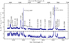 |
Fig. 1. Top panel: Reduced optical spectra of WPVS 48 during the variability campaign from December 2013 to June 2014. The spectra were calibrated to the same absolute [O III] λ5007 flux of 244 × 10−15 erg cm−2 s−1. The identified emission features are labelled. Bottom panel: Zoomed-in image of the continuum and the low-intensity emission lines. The conspicuous feature at ∼5490 Å is a residual from night-sky emission. |
Figure 2 shows the composite mean and rms spectrum from the intercalibrations (see Sect. 2) shortward and longward of 5645 Å, respectively34. The division line between the two spectral regions is indicated by a grey dashed line. The rms spectrum is scaled by a factor of × 25 to facilitate a straightforward comparison. We highlight the line-free continuum regions analysed in this work with light blue lines below the spectrum as well as the Balmer and Helium lines with the corresponding integrated line flux. The spectral region used to measure the integrated line flux was chosen such that it encompasses the total variable component of the emission lines, which can be deduced from the rms spectrum. The specific continuum boundaries, integration limits and selected pseudo-continua are given in Table 2. This work focuses on the Balmer as well as He Iλ5876 and He IIλ4686. A detailed analysis on the remaining He I lines will be given in a following publication (Probst et al., in prep.).
Continuum boundaries and line integration limits (2) as well as the sections used to fit the pseudo-continua (3).
3.1.1. Host galaxy contribution
We estimate the contribution of the host spectrum in the B, V and R band of the spectra applying the flux variation gradient (FVG) method (Choloniewski 1981; Winkler et al. 1992; Kollatschny et al. 2022). We adopt typical host slopes in the B − V and B − R colour indexes found by Sakata et al. (2010) and Haas et al. (2011), respectively. We determine the colour indices in WPVS 48 using line-free continuum emission that has an effective wavelength (in the observed frame) close to the one of the corresponding filters employed by Winkler et al. (1992), Sakata et al. (2010) and Haas et al. (2011). We hence select the continuum regions Cont. 4440, Cont. 5100 and Cont. 6250 for the B, V and R band, respectively. The three selected continuum regions have a respective effective wavelength of 4605 Å, 5290 Å and 6480 Å. Figures 3 and 4 show the AGN slope and the typical host slope in the B − V and B − R colour plots. From the intersection of the slopes, we determine host fluxes of 0.08 mJy (mean of 0.06 and 0.10 mJy), 0.24 mJy and 0.18 mJy in the B, V and R band, respectively, and thus a host contribution of 3 − 12%. The flux densities in units of mJy and erg cm−2 s−1 Å−1 for the combined as well as the separated AGN and host contributions in the three bands are given in Table 3.
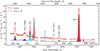 |
Fig. 2. Combined mean spectrum (black) and rms spectrum (red) of WPVS 48 from our campaign. The partition in the two intercalibrations (see Sect. 2 for details) is shown with a grey dashed line. The rms spectrum was scaled to allow for a direct comparison. The analysed continuum regions and the identical pseudo-continua used for linear continuum subtraction are highlighted with blue bars below the spectra. The line integration limits are marked by the shaded areas. All emission lines of He I are displayed in orange. |
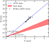 |
Fig. 3. Extinction corrected B-V flux variations. The blue dashed line represents the best linear fit of the AGN slope of WPVS 48 and the red shaded area the host slopes of nearby AGN. |
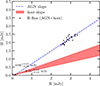 |
Fig. 4. Extinction corrected B-R flux variations. The blue dashed line represents the best linear fit of the AGN slope of WPVS 48 and the red shaded area the host slopes of nearby AGN. |
Extinction-corrected B, V, and R values for the combined host galaxy plus AGN fluxes, and for the host galaxy and AGN fluxes alone, as determined by the FVG method.
No stellar signature is discernable in any of our taken spectra. Specifically, no stellar absorption lines are visibly superposed with the AGN emission. Hence, we did not subtract any possibly remaining host flux. A subtraction is also not necessary, as any constant host flux has no effect on the estimate of the BLR size by means of RM in the following analysis.
3.1.2. Identification of Bowen fluorescence near He II λ4686
Additionally to the line identification shown in Fig. 1, we analyse the spectral region close to He IIλ4686 in more detail in Fig. 5. Specifically, in the blue wing of He IIλ4686, two broad peaks are conspicuous. The wavelength of the peaks match to N IIIλ4640 and C IVλ4658, which together with He IIλ4686 are often referred to as Wolf-Rayet feature and was interpreted in the past as the presence of a high number of Wolf-Rayet stars in the host galaxy (e.g. Osterbrock & Cohen 1982). The feature has also been seen in tidal disruption events (Gezari et al. 2015; Brown et al. 2018, 2017) as well as a new type of transient event in AGN defined by Trakhtenbrot et al. (2019) with distinctively strong He II emission. Specifically, the He II emission at 303.78 Å produces the Bowen-fluorescence lines in multiple N III lines including N IIIλ4640 (Netzer et al. 1985; Trakhtenbrot et al. 2019, and references therein). To distinguish the Wolf-Rayet feature from emission of the Fe II emission, we mark the wavelength range of Fe II (37, 38) multiplets as given in the template of Park et al. (2022). Further, we mark two peaks in the red wing of He IIλ4686, whose wavelengths match the [Ar IV] λλ4712, 4740 lines.
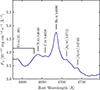 |
Fig. 5. Detailed emission line identification in the mean spectrum close to He IIλ4686. We identify N IIIλ4640 and C IVλ4658 (Osterbrock & Cohen 1982) and further labelled the position of the Fe II (37, 38) emission bands (for a template of Fe II, see Park et al. 2022) as well as [Ar IV] λλ4712, 4740. |
3.2. Continuum variability
3.2.1. Continuum light curves
We present the light curves of the continuum flux densities at 4265 Å, 4440 Å, 4775 Å, 5100 Å, 5760 Å, 6030 Å, 6250 Å, 6810 Å, 7030 Å, 7110 Å (rest wavelength) in Fig. 6. The continuum bands were selected such that they are not contaminated with emission lines. The selected continua are equivalent to line-free continuum bands identified in previous spectroscopic continuum RM campaigns (e.g. Kollatschny et al. 2001; Cackett et al. 2018; Zhou et al. 2025). The presented light curves are measured within the integration limits given in Table 2. All measured light curves have a similar overall shape with a sequence of (1) a short duration of higher flux, (2) a steep decline and a short period of lower flux, (3) an increase in flux marking the beginning of a second, longer period of increased flux and (4) a second decline. Notably, the flux ratio of both periods of high flux is ∼1 for the blue continua, whereas the flux of the second period is ∼10 percent lower for the red continua. The flux densities of the measured continua are tabulated in B.1. We derive the minimum and maximum fluxes Fmin, Fmax, peak-to-peak amplitudes Rmax = Fmax/Fmin, mean of the measured flux (densities) ⟨F⟩, the standard deviation σF, and the fractional variation,
 (1)
(1)
as defined by Rodríguez-Pascual et al. (1997), for the presented continuum light curves. Here, Δ2 denotes the mean square value of the uncertainties of the individual fluxes Fi of the light curve. The calculated values are tabulated in Table 4 and show that the mean flux density, the variability amplitude and the fractional variation decrease with increasing wavelength.
Variability statistics of the investigated continua and emission lines with minimum (2) and maximum flux density or integrated flux (3), peak-to-peak ratio (4), mean flux density (5), standard deviation (6), and fractional variation (7).
3.2.2. Interband continuum delays: Univariate analysis
We correlate the continuum light curves with the light curve of the continuum at 4265 Å, thereby determining interband continuum time lags with respect to the bluest continuum of this work. The univariate model underlying this analysis of interband continuum delays assumes similar, albeit shifted light curves conjectured to stem from an irradiated accretion disk (compare with e.g. Collier et al. 1998), such that
 (2)
(2)
for two continuum light curves in a bluer band Fb and a redder band Fr. In this equation, τ is the lag between the two light curves.
The employed correlation technique is the interpolated cross-correlation function (ICCF) described by Gaskell & Peterson (1987). We calculate interband continuum lags according to both the peak τpeak and the centroid τcent of the cross-correlation function. For the calculation of the centroid of the CCF, only values above 80 percent of its peak value rmax are considered. As demonstrated in Peterson et al. (2004), a threshold value of 0.8 rmax is generally a good choice.
We derive the uncertainties by calculating the peak and the centroid lag for ∼20 000 runs in a model-independent Monte-Carlo method known as flux randomisation/random sub-sample selection (FR/RSS). The method is described in detail by Peterson et al. (1998). The errors are evaluated using the centroid and peak distributions such that 68% of the realisations yield values between the error interval.
The calculated lags are given in Table 5. Figure 7 shows the mean centroid lags as function of the effective wavelength of the respective continuum band and Fig. A.1 shows the individual correlation functions and the corresponding centroid distributions. The mean centroid time lag τcent is ∼0 days for the continua in the B band including the continuum at 5100 Å. The lag jumps to ∼5 days between the continua measured at 5100 Å and 5775 Å and continuously increases up to ∼8 days for continua in the R band.
Interband cross-correlation lags τ with respect to the continuum at 4265 Å (at 4425 Å in observed frame) as well as the maximum correlation coefficient rmax and the fractional contribution α of the secondary component, respectively, for the univariate and bivariate model.
We repeated the calculation for the photometric V band and R band light curves of Sobrino Figaredo et al. (2018) with respect to the continuum at 4265 Å from this work. The derived centroid lags of the V band and R band light curves amount to 5.4−1.9+1.6 and  days, respectively, and are consistent with the interband continuum lags described above. The photometric light curves were obtained with the VYSOS-6 and BEST-II telescopes of the Universitätssternwarte Bochum near Cerro Armazones in the time period between December 2013 and May 2014. Hence, the photometric light curves overlap with the spectroscopic light curves from this work. The derived lags are included in Fig. 7 as grey squares. We note that the photometric V band light curve may have contributions of variable line emission, especially Hβ and He Iλ5876, which may shift the measured lag to larger delays. In 4.1.1, we compare our red continuum light curve with the independent observations of Sobrino Figaredo et al. (2018).
3.2.3. Interband continuum delays: Bivariate analysis
In addition to the univariate model, a different interpretation exists allowing an additional secondary component from a diffuse continuum originating from the BLR (Korista & Goad 2001). Therefore, we perform an additional analysis using a formalism by Zucker & Mazeh (1994) adapted for a bivariate model of interband continuum delays by Chelouche & Zucker (2013). The bivariate model assumes that the delayed red continuum light curve can be reconstructed with two identical superposed components of the blue continuum light curve. The primary component is not delayed, whereas the secondary is5. This yields
 (3)
(3)
where α denotes the fractional contribution of the delayed component.
We correlate the red-band light curve with a superposition of the non-delayed and delayed blue-band light curves under varying contributions and lags. We derive the fractional contributions α and delays τsec from the correlation with the highest correlation coefficient. The retrieved lags τsec and contributions α with respect to the continuum light curve at 4265 Å (4425 Å in observed frame) are tabulated in columns 5 and 6 of Table 5 and plotted in Fig. 7. We repeated the analysis in ∼20 000 Monte-Carlo simulations employing both FR and RSS to evaluate the uncertainties. We note that we exclude the continua at 4440 Å and 4775 Å, which is discussed in Sect. 4.1.3.
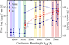 |
Fig. 7. Mean centroid lags τcent according to the univariate model (blue squares) as well as centroid lags τsec (blue circles) and fractional contribution α (red circles) of the secondary component according to the bivariate model (Chelouche et al. 2019) as a function of the effective wavelength of the continuum. We include the univariate lags of photometric light curves published by Sobrino Figaredo et al. (2018) as grey squares. We note that Hβ contributes to the flux in the V band. The lags and the fractional contribution are measured with respect to the continuum at 4265 Å as a function of the effective wavelength of the continuum. The colouring of the shaded background corresponds to the light curves in Fig. 6. The errors correspond to the 68% (±1σ) confidence level after a Monte-Carlo simulation with 20 000 runs. The data of τsec and α have been slightly shifted in wavelength for better readability. |
The results are consistent with a contribution of the secondary delayed component with a lag of 11–15 d. This contribution increases with higher wavelengths from α ≈ 0.2 for the continuum at 5100 Å to α ≈ 0.5 for the continuum at 7030 Å.
3.3. Emission-line variability
3.3.1. Broad-line fluxes and light curves
We present the light curves of the integrated line fluxes of the Balmer lines as well as the He Iλ5876 and He IIλ4686 lines in Fig. 8. We evaluate the line fluxes after the subtraction of a linear pseudo continuum. The flux integration limits as well as the regions used to interpolate the pseudo continua are given in Table 2. The emission-line light curves show a similar sequence as the continuum light curves described in Sect. 3.2.1. The flux ratio between the two periods of high flux is ∼1 as observed in the light curves of the bluer continua. The fluxes of the measured lines are tabulated in B.2. We derive the minimum and maximum fluxes Fmin, Fmax, peak-to-peak amplitudes Rmax = Fmax/Fmin, mean of the measured flux (densities) ⟨F⟩, the standard deviation σF, and the fractional variation analogously to the continuum light curves. The calculated values for the emission-line light curves are tabulated in Table 4. The variability amplitudes and fractional variation are higher for He IIλ4686 and He Iλ5876 than for the Balmer lines.
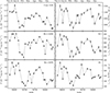 |
Fig. 8. Emission line light curves of the Balmer lines as well as He Iλ5876 and He II λ4686 measured within the integration limits given in Table 2. The continuum light curve at 5100 Å is included for reference. |
3.3.2. Emission-line lags and BLR size
We correlate light curves of the integrated emission lines with the light curve of the continuum at 5100 Å, thereby determining the mean light travelling time from the ionising source to the variable broad component of the emission lines. Commonly, the continuum at 5100 Å is used as a surrogate for the light curve of the ionising continuum in variability studies.
In some previous RM campaigns analysing interband continuum delays, the B band continuum light curves are, firstly, higher-correlated with the ionising UV continuum (e.g. Edelson et al. 2019), and, secondly, exhibit shorter delays to the ionising UV/X-ray continuum than the V band (e.g. Edelson et al. 2015; McHardy et al. 2018; Zhou et al. 2025). We, therefore, correlate the emission line light curves also with the bluest line-free continuum region at 4265 Å in our spectra. This continuum region was specifically selected because it is free from contamination of both Fe IIλ4233 and Hγ.
The employed correlation technique as well as the uncertainty estimation (FR/RSS) are the same as for the interband continuum delays described in Sect. 3.2.2. The correlation functions and the centroid distributions resulting from the Monte-Carlo method employing FR/RSS are shown in Fig. 9. The derived lags are tabulated in Table 6.
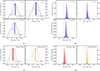 |
Fig. 9. Left panels: CCFs of the integrated Balmer lines in blue, the integrated He I λ5876 line in orange and the integrated He II λ4686 line in red, with respect to the continuum light curve at 5100 Å. The time lag, τcent, is denoted by a dashed line; the shaded area corresponds to a ±1σ interval from the Monte-Carlo simulations. Right panels: Cross-correlation centroid distributions after 20 000 runs employing FR and RSS of the integrated Balmer lines in blue, the integrated He I λ5876 line in orange and the integrated He II λ4686 line in red, with respect to the continuum at 5100 Å. |
Cross-correlation lags of the continuum light curves at 4265 Å and 5100 Å (at 4425 Å and 5290 Å in observed frame, respectively) with the light curves of the integrated lines.
The light curves are well correlated with maximum correlation coefficients between 0.74 and 0.9 for the correlations with both continua. We determine centroid lags of the Balmer lines Hα and Hβ of ∼16 days, consistent with the Hα lag of ∼18 days found by Sobrino Figaredo et al. (2018) based on photometry with a narrow-band filter. Further we derive centroid lags of ∼12 days and ∼14 days for Hγ and He Iλ5876, respectively. Notably, the lag of He Iλ5876 is identical to the lags of the Balmer lines within the errors. The corresponding centroid lags from correlations with both continua are consistent for aforementioned lines and deviate by ≲1.5 days. The centroid lag of He IIλ4686 is close to the minimum sampling in this campaign and amounts to ≲5 days.
3.3.3. Broad-line profiles
Figure 10 shows the normalised mean and rms profiles of the Balmer lines as well as of the He Iλ5876 and He IIλ4686 lines after subtraction of a linear pseudo-continuum with the wavelengths indicated in Table 2. In order to retrieve genuine mean line profiles without the contribution of forbidden narrow lines, we corrected the mean profiles of Hα and Hγ for [N II] λλ6548, 6584 and [O III] λ4363, respectively, by subtracting a scaled narrow-line template of [O III] λ5007. The uncorrected line profiles of Hα and Hγ are also indicated in Fig. 10 with a grey dashed line. We did not subtract the narrow components of the Balmer and Helium lines, as the broad component is only slightly broader than the narrow component, and the narrow components thus cannot be unambiguously separated using a narrow-line template of [O III] λ5007. The rms profiles reflect only the variable broad component, but not the constant narrow component of the line. We note that the closest line-free region blueward of He IIλ4686 is at ≈4440 Å beyond the Fe II emission band. Therefore, the blue wing of the He IIλ4686 mean profile does not reach the base line.
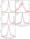 |
Fig. 10. Normalised mean (black) and rms (red) line profiles of the Balmer and the prominent He Iλ5876 and He IIλ4686 emission lines. While the mean profiles corrected for contributions of narrow forbidden lines are shown in red, the grey dashed line indicates the uncorrected mean profiles of Hα and Hγ. We note that the blue wing of the mean He IIλ4686 profile blends with emission from N IIIλ4640, C IVλ4658, and Fe II (37, 38) multiplets. |
We compare the mean and rms profiles of the Balmer lines with each other and with He Iλ5876 as well as He Iλ5876 with He IIλ4686 in Fig. 11. We note nearly identical and nearly symmetrical mean profiles of the Balmer lines and He Iλ5876 with the profiles of Hγ and He Iλ5876 being slightly broader (line widths and corresponding lags are discussed in Sect. 4.2). The blue wings of the Balmer lines do not reach the base line due to blends with adjacent lines. We note higher flux at the wings of the mean profile of He Iλ5876 at ∼ − 4700 km s−1 and between ∼ + 2500 and ∼ + 7300 km s−1, which is not present in the Balmer profiles.
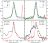 |
Fig. 11. Top panels: Comparison of the normalised mean (left panel) and rms (right panel) line shapes of the Balmer emission lines with the He Iλ5876 emission line. Bottom panels: Comparison of the normalised mean (left panel) and rms (right panel) line shapes of the He Iλ5876 emission line with the He IIλ4686 emission line. We note that the blue wing of the mean He IIλ4686 profile blends with emission from N IIIλ4640, C IVλ4658, and Fe II (37, 38) multiplets. |
The Balmer lines and He Iλ5876 exhibit similar rms line shapes with FWHM of ∼1500 km s−1, which furthermore are nearly symmetrical with exception of the peak. Specifically, all lines show a flux deficit at the upper 20% of the blue wing resulting in a redward asymmetry of the rms peaks. The redshift of the peaks in the rms profiles with respect to the peaks in the mean profiles are equal and amount to ≈300 ± 100 km s−1 with variations of the order of the spectral resolving power of RSS with a PG900 grating.
The He IIλ4686 line with a FWHM of ∼4000 km s−1 is clearly broader than the Balmer lines and the He Iλ5876 emission. Comparing the two Helium lines, He IIλ4686 exhibits a similar redshift of its rms profile peak as He Iλ5876 (and the Balmer lines). The red wing of He IIλ4686 declines steadily without apparent features (except the blends with [Ar IV] λλ4712, 4740 in the mean profile). The blue wing of He IIλ4686, however, is extended in both the mean and rms profiles due to the line blends described in Sect. 3.1.2.
We measured the line widths (full width at half maximum, FWHM) of the Balmer lines as well as He Iλ5876. Furthermore, we parametrised the line widths by means of the line dispersion (Fromerth & Melia 2000; Peterson et al. 2004). The measurements for Hα and Hγ are performed for the line profiles corrected for the narrow-line contributions of [N II] λ6548, [N II] λ6584 and [O III] λ4363, respectively. In order to minimise the effect of further blended lines located on the extreme wings to the line dispersion, we limited the evaluation of the line dispersion only to the variable spectral ranges given in Table 2. This also encompasses the majority of the flux of the mean profiles.
As a result, we measured FWHM without and line dispersions with minimal effect of line blends for the mean and rms profiles of the Balmer lines and He Iλ5876. This, however cannot be stated for He IIλ4686: Due to the prominent narrow component in He IIλ4686, the half maximum is likely overestimated, and thus the measured FWHM is likely underestimated. Both the FWHM of the rms profile as well as the line dispersion of both profiles include the extended blue wing, and thus the emission from N IIIλ4640 and C IVλ4658. For the total line complex, we measure a FWHM of (5060±660) km s−1. Due to the blends, we only give the width of the red wing of the rms profile alone, which amounts to 1780 km s−1. We base the estimate of the uncertainties of the line widths on the bootstrap method described in Peterson et al. (2004).
3.3.4. Narrow-line fluxes
We measure the constant fluxes of the narrow forbidden lines [O III] λ4959, [O III] λ5007, [O I] λ6300, [O I] λ6364 as well as the combined flux of [S II] λλ6716, 6731, in the intercalibrated extinction-corrected spectra. We present mean values of the measured fluxes alongside with the standard deviations as errors in Table 8. We determine the fluxes of the narrow lines [O III] λ4363, [N II] λ6548 and [N IIλ6584] based on the flux of [O III] λ5007 and the respective factors (0.021, 0.063 and 0.201) from the decomposition of the line blends with Hα and Hγ in their mean profiles as explained in Sect. 3.3.3. Here, we assume an uncertainty in the multiplicative factor of 0.01, which translates to a flux uncertainty of 2.5 × 10⁻¹⁵ erg cm−2 s−1.
FWHM and line dispersion σline of the mean and rms profiles of the Balmer lines and He Iλ5876.
Line intensities of the narrow forbidden lines.
3.4. Black hole mass estimation and bolometric luminosity
We estimate the BH mass from reverberation mapping data using the following equation:
 (4)
(4)
This estimate is based on the assumption that the gas dynamics are dominated by the central black hole. In our study, we use τcent with respect to the continuum at 5100 Å (see Sect. 3.3.2) to estimate the mean distance of the origin of the variable line emission to the ionising continuum source and the FWHM of the rms profiles to parametrise the mean velocities in the variable gas (see Table 7). The scaling factor f accounts for the geometrical distribution of the gas to the line of sight and various values of the order of unity have been discussed in literature (e.g. Onken et al. 2004; Graham et al. 2011; Grier et al. 2013a) for samples of AGN. The value for individual AGN, however, may differ from the values derived from these samples. The narrow width of the broad line components may originate from either a low-mass BH or a face-on geometry of WPVS 48. A face-on geometry would likely lead to a high f value (e.g. Krolik 2001; Labita et al. 2006; Decarli et al. 2008). Therefore, we give only the virial product c τ Δv2 G−1 in this section and discuss the scaling factor f and the BH mass in Sect. 4.3.
The virial products for the individual emission lines based on both the FWHM and σline and the lag to the continuum at 5100 Å are given in Table 9. Here, we exclude He IIλ4686 from the estimate, as the deblended line profile is difficult to obtain. The virial products based on the FWHM are consistent with each other, their weighted mean of the amounts to
 (5)
(5)
Virial products based on reverberation mapping.
The errors are propagated from both the high errors in the estimate of the line width as well as the lag from the CCF.
We, furthermore, used the mean continuum flux density of Fλ = (2.68 ± 0.22)×10−15 erg cm−2 s−1 Å−1 at 5100 Å to infer the optical luminosity of λL5100 = (4.74 ± 0.39)×1043 erg s−1. Here, we adopt the bolometric correction factor of ∼19.9 from Netzer (2019, see their Equation 3 and Table 1)
![Mathematical equation: $$ \begin{aligned} k_{\text{bol}} = 40 \times [\lambda L_{5100} / 10^{42}\,\text{ erg}\,\text{ s}^{-1}]^{-0.2}, \end{aligned} $$](/articles/aa/full_html/2026/02/aa54969-25/aa54969-25-eq83.gif) (6)
(6)
and derive a bolometric luminosity of Lbol = (8.76 ± 0.72)×1044 erg s−1.
4. Discussion
4.1. Optical variability
4.1.1. Comparison to the photometric campaign
We compare the intercalibration of the spectroscopic data redward of 5645 Å with the independent calibration by Sobrino Figaredo et al. (2018). Figure 12 shows the continuum light curve at 6810 Å of this work as well as the R band light curve from Sobrino Figaredo et al. (2018) after the subtraction of a constant flux density of 1.57 × 10⁻¹⁵ erg cm−2 s−1 Å−1. The continuum at 6810 Å was chosen for the comparison, as it is closest to both the [S II] λλ6716, 6731 emission and the effective wavelength of the employed R band filter in the rest frame of WPVS 48. We are able to reproduce the photometric light curve of Sobrino Figaredo et al. (2018) well with our spectroscopic light curve. Most importantly, we are able to reproduce the variability amplitude without employing a multiplicative factor to our calibrated light curve. The necessary subtraction of flux density is likely be explained with the larger aperture with a diameter of of 7 5 that was used in the photometric observations.
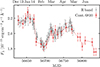 |
Fig. 12. Comparison of the spectroscopic continuum light curve at 6810 Å and the photometric R band light curve from Sobrino Figaredo et al. (2018) (effective wavelength in the rest frame of WPVS 48 λeff = 6750 Å), shifted by −1.57 × 10⁻¹⁵ erg cm−2 s−1 Å−1. |
4.1.2. Spectral continuum slope
We now test whether the spectral index of the optical continuum is consistent with the theoretical predictions from accretion disk models – specifically, the spectral energy distribution of the UV/optical continuum from Shakura & Sunyaev (1973), which is commonly used as first-order approximation in AGN (e.g. Davis et al. 2007; Kishimoto et al. 2008), although the details are more complex (e.g. Blaes et al. 2006; Antonucci 2023, and references therein). The Shakura & Sunyaev model predicts a flux density scaling with frequency like Fν ∝ ν1/3 for the spectral region unaffected by contributions from the inner and outer AD that radiate in the UV and infrared, respectively. A spectral index of α = 1/3 translates to a spectral slope of β = −7/3, as Fλ = Fνdν/dλ ∼ ν1/3ν2 ∼ λ−7/3.
Figure 13 shows a logarithmic plot of the observed rms spectrum corrected for Galactic foreground extinction. As the bivariate model for the interband continuum delays (see Sect. 3.2.3) suggests a major secondary contributor other than the AD to the continuum at 5760 Å and higher wavelengths, we fit the spectral continuum slope twice: The first fit considers the blue continua only, i.e. at 4265 Å, 4400 Å, 4775 Å and 5100 Å, whereas the second fit includes all continuum regions discussed in this work: The first fit gives β = 2.61 ± 0.06 and is fairly consistent with the theoretical prediction of the Shakura & Sunyaev model given that we test this relation over a limited wavelength range only. However, the inclusion of the continua at higher wavelengths results in a redder continuum slope, which yields β = 1.86 ± 0.02. The break between the two power laws is close to Hβ and coincides with the jump in the measured univariate interband continuum delays. While the presence of a secondary continuum emitter is a possible explanation of this break in power law, we cannot exclude the host contribution being responsible for the break.
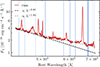 |
Fig. 13. The rms spectrum of the SALT campaign corrected for Galactic foreground extinction (red). Two power-law models are fitted to the continuum slope. The first considers only the continua at 5100 Å and bluewards giving a spectral index β = 2.61 ± 0.06 (black); the second considers all measured continua giving a spectral index β = 1.82 ± 0.03 (grey). |
4.1.3. Interband continuum delays
In Sect. 3.2.2, we present interband continuum delays that increase with wavelength. Specifically, we calculate lags of 2–3 days between continua corresponding to the V and R band consistent with the lags ≲3 days discussed in other studies that include these wavelength bands (e.g. Fausnaugh et al. 2016; Cackett et al. 2018; Chelouche et al. 2019; Hernández Santisteban et al. 2020; Kara et al. 2021; Vincentelli et al. 2021). The calculated lag between the B and the R band of ∼7 days in this work is rather high compared to the lags of ∼1.5–4.1 measured in other campaigns (e.g. Fausnaugh et al. 2016; Hernández Santisteban et al. 2020; Kara et al. 2021; Vincentelli et al. 2021; Zhou et al. 2025). Given the good agreement of our spectroscopic light curve with the photometric light curve of Sobrino Figaredo et al. (2018) (see Sect. 4.1.1), we argue that the intercalibration performed in this work did not lead to the high lag. However, we note that the referenced studies that include observations in both the B and the R band are based on photometric broad-band data. The separation of continuum and line contribution is not straightforward in photometric data, whereas for the spectroscopic data of this work a separation of continuum and line flux is achieved. Therefore, the line contribution in the previous studies might have led to higher lags in the B band as discussed in Chelouche et al. (2014), thereby decreasing the lag between the B and the R band.
In Sect. 3.2.3, we probed the scenario of a secondary variable continuum emitter located further away to the central source that – similar to the emission lines in the B band – might result in longer delays: Such diffuse continuum emission from the BLR has been proposed for instance by Korista & Goad (2001) and Chelouche et al. (2019). We repeated the model calculations with various ICCF samplings of 0.5, 2 and 4 days. For continuum light curves whose univariate lag is comparable to the sampling of the campaign – i.e. the continua at wavelengths ≥5100 Å – this test results in the same lags τsec and contribution factors α for the secondary component. However, the test struggles to find consistent delays for the continua with univariate delays far below the sampling, i.e. Cont. 4440 and Cont 4775. For this reason, we exclude the latter continua from the bivariate analysis.
For the remaining continua, we are able to model the measured delays with a contribution of a secondary component with a lag of 11–15 days. This contribution increases with wavelength to up to ∼50 percent. Intriguingly, the lag of the secondary continuum component matches the lags of Hα, Hβ, Hγ and He Iλ5876, pointing at a diffuse continuum component that originates in the Balmer BLR. In their continuum RM study on Mrk 279, Chelouche et al. (2019) measured the continuum flux with intermediate-band filters (≃100 Å-wide) at 4300 Å, 5700 Å, 6200 Å and 7000 Å. They interpreted the continuum delays with the bivariate model; however, the measured lag of the secondary continuum component in Mrk 279 indicates an origin that is five times closer to the central source than the Balmer BLR. Furthermore, the contribution of the secondary component is higher throughout all examined intermediate-band filters ranging between 70 and 90 percent.
Comparing the two campaigns, we note a much higher sampling rate of ≲1 day for the observations of Mrk 279. In case of WPVS 48, lags that are five times smaller than the Balmer lags, i.e. 2–3 days, are in fact below the average sampling rate of our campaign. This hinders the ability of the bivariate model to distinguish two continuum signals 2–3 days apart delay-wise, as is described for the continua at 4440 Å and 4775 Å above. Furthermore, the light curves have a different variability pattern in both AGN: Mrk 279 exhibits non-monotonic continuum variability on timescales of ∼5 days, whereas the continuum light curves of WPVS 48 show non-monotonic continuum variability on timescales of ∼20 days. This observation of variability on different timescales cannot be accounted for the lower sampling rate of our campaign alone, as the same holds true for the higher-sampled photometric light curves of Sobrino Figaredo et al. (2018, see Fig. 12). Thus, different dominant secondary continuum components may be observed due to different sampling rates or due to distinct variability behaviours of the AGN.
In addition to optical interband continuum lags, lags between the highly ionising continuum in the UV/X-ray and optical continua were measured in other galaxies: Specifically, the RM studies on NGC 4151 (Edelson et al. 2019), NGC 4593 (Cackett et al. 2018; McHardy et al. 2018; Edelson et al. 2019), NGC 5548 (Edelson et al. 2015; Fausnaugh et al. 2016; Edelson et al. 2019), Fairall 9 (Hernández Santisteban et al. 2020; Edelson et al. 2024), Mrk 110 (Vincentelli et al. 2021), Mrk 509 (Edelson et al. 2019) and Mrk 817 (Kara et al. 2021) include wavelength bands of the highly ionising continuum in the UV or X-ray. They found typical lags between UV/X-ray and V band continua ranging from 0.48 to 4.3 days6.
4.1.4. Emission line variability
In Sect. 3.3.2, we deduce the BLR size for various emission lines from the CCFs with two optical continuum light curves. While the inferred sizes for the Balmer lines and the He Iλ5876 line (ranging between ∼11 and ∼16 days) from the CCFs with both continua agree with each other, the CCFs for He IIλ4686 result in BLR sizes that – depending on the chosen continuum – differ by a factor of ∼2. Specifically, the derived BLR sizes for He IIλ4686 range between 2 and 5 days. Here, a similar argument can be made as with the continuum light curves in Sect. 4.1.3: As the found lag is below the sampling rate, the delays resultant from the cross correlations differ.
The He IIλ4686 line is furthermore blended with N IIIλ4640 and C IVλ4658. The extended blue wing of He IIλ4686 points at variability in either or both of the blended lines. Variable N IIIλ4640 emission have been observed in flaring AGN so far (Trakhtenbrot et al. 2019; Makrygianni et al. 2023, and references therein). However, no flaring in WPVS 48 is known to the authors. We hence show that the Bowen fluorescence line N IIIλ4640 is also present in non-outburst spectra.
4.1.5. Balmer decrement variability
We calculate the Balmer decrement Hα / Hβ for all epochs. Figures 14 and 15 show the relation to the measured continuum flux density at 5100 Å and the Hβ flux, respectively. We subtracted the flux of the narrow-line component before the evaluation of the Balmer decrement. The narrow-line fluxes (17.8 erg cm−2 s−1 and 39.3 erg cm−2 s−1 for Hβ and Hα, respectively) have been estimated with the help of a higher-resolved X-shooter spectrum (PI: Benny Trakhtenbrot, Program ID: 109.22YE) from 2022, i.e. 8 years after the SALT campaign. We thereby assume that the broad line profiles remain largely unchanged over this time period, which we test with an overplot of the line profiles from the X-shooter spectrum and the mean SALT spectrum. Both line profiles previously have been corrected for the narrow component using [O III] λ5007 as a template. We repeat the process with for the SALT spectrum employing different scaling factors for the narrow-line correction and conclude that for flux differences of ±2.5 erg cm−2 s−1 clear residuals of the narrow components emerge in the difference spectrum. We, therefore, adopt this as the uncertainty of the narrow component.
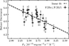 |
Fig. 14. Balmer decrement, F(Hα)/F(Hβ), of the broad-line components vs continuum intensity at 5100 Å. The dashed line on the graph represents the linear regression. |
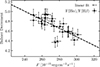 |
Fig. 15. Balmer decrement, F(Hα)/F(Hβ), of the broad-line components vs broad-line Hβ intensity. The dashed line on the graph represents the linear regression. |
The values of the Balmer decrement are between 4.3 and 5 and show a roughly linear relation with the continuum flux density and the Hβ flux, precisely, the Balmer decrement decreases with increasing flux (density). Similar Balmer decrements ranging between ∼3 and ∼5 have been measured in other AGN, such as NGC 7603 (Kollatschny et al. 2000), HE 1136-2304 (Kollatschny et al. 2018), and Mrk 926 (Kollatschny et al. 2022). For instance, the slope of the Balmer decrement in WPVS 48 is similar to that of NGC 7603 in epochs of higher Hβ flux (F ≳ 250 erg cm−2 s−1), whereas the slope in NGC 7603 becomes steeper and the Balmer decrement reaches ∼7 for epochs with lower Hβ flux (F ≲ 250 erg cm−2 s−1). Korista & Goad (2004) simulated the responsivities of the optical emission lines prominent in AGN in relation to the incident flux and suggested that the found behaviour of the Balmer decrement as well as the apparent stratification of the BLR may be explained with optical depth effects.
4.2. Emission line profiles
In Sect. 3.3.3, we extract the broad rms profiles of the Balmer lines and He Iλ5876. The extracted rms profiles of Hβ, Hα and He Iλ5876 measure almost equal line widths of ∼1500 km s−1. While the bootstrap method employed to assess the uncertainties of the line widths accounts for noise in the line profiles, it does not account for systematic biases from the presence of a potential narrow component. Since a robust line-profile decomposition is hard to achieve for NLS1s due to blending of the narrow and broad components, we tested the influence of a possible narrow-line residuum in the upper 10% of the rms peaks by measuring the width at the flux level of 0.45 of the maximum. A narrow-line residuum of the order of 10% of the peak flux would broaden the FWHM of the rms profiles by ∼130 km s−1. Such a residuum, however, is not conspicuous in the rms profiles and we, therefore, conclude that such bias is smaller than ∼130 km s−1 and the uncertainties already given in Sect. 3.3.3.
The similar width suggests that all four lines originate from roughly the same distance to the central source, which is corroborated by the lag measurements in Sect. 3.3.2. Line widths and lags consistently reflect small differences in the distance from the central source, as Hγ and He Iλ5876 have both smaller lags and slightly higher widths than Hβ and Hα. All four lines furthermore show a similar line shape, which includes the same feature of a slight redward asymmetry in their rms peaks (upper 20%). A redward asymmetry is furthermore present in the rms peak of He IIλ4686. The appearance of this feature in all five lines suggests that this line feature is genuine and not a result from the reduction or intercalibration process.
Redward asymmetries have been observed in multiple AGN and have been reproduced using different models, for instance: Ochmann et al. (2024) fitted the double-peaked Ca IIλ8662 with a redward asymmetry profile of NGC 1566 with the model by Eracleous et al. (1995) of the emission of an elliptical accretion disk at an inclination angle of i ≈ (8.1 ± 3.0)°. The single-peaked Hβ profile showing a redward asymmetry has then been replicated from the Ca IIλ8662 profile by adding turbulence. Kollatschny (2003b) suggested gravitational redshift as an explanation for the redshifted rms peaks in the NLS1 Mrk 110 and inferred an inclination angle of i ≈ (21 ± 5)°. Goad et al. (2012) presented a series of line profiles expected from their disk model and linked redward asymmetries to the combined effect of gravitational redshift, transverse Doppler shift and turbulence. Specifically, they concluded that these effects on line profiles are apparent only in near face-on systems (i ≲ 20°). While the combination of relatively narrow widths in the BLR components and a redward asymmetry in the rms profile is consistent with a low inclination angle in these models, we note that there is no estimate of the inclination angle based on the presence of both features alone. The scaling factor f, therefore, is unconstrained by this observation and both the low-inclination and the low-mass scenario of the AGN in WPVS 48 are equally possible.
We now infer (projected) rotational vrot and turbulent velocity components vturb in the BLR from the FWHM and the line dispersion σline following the model of Kollatschny & Zetzl (2011, 2013). The model parametrises rotationally broadened Lorentzian profiles, which are associated with turbulent motion (see also Goad et al. 2012) in terms of the FWHM and the FWHM / σline ratio. This way, Kollatschny & Zetzl (2011, 2013) were able to identify characteristic turbulent velocities in various emission lines of AGN. Based on the rotational and turbulent velocities, we calculate the ratio of the height above the midplane to the radius of the line emitting regions H/R as presented in Kollatschny & Zetzl (2011, 2013).
 (7)
(7)
where the viscosity parameter is assumed to be in the range between 0.1 and 1 (e.g. Frank et al. 2002). For simplicity, we adopt α = 1. The calculated values for vturb, vrot and H/R are given in Table 10. We note, however, that the model of Kollatschny & Zetzl (2011, 2013) does not account for a low inclination angle or relativistic effects. In fact, Kollatschny & Zetzl (2013) point out that NLS1s tend to have lower FWHM while having FWHM / σline ratios similar to broad-line Seyfert galaxies. A lower estimate of the line dispersion implies a lower turbulent velocity, and thus a lower scale height.
Inferred velocities of (projected) rotational and turbulent motion as well as scale height of the prominent emission lines.
4.3. Inclination angle, central black hole mass and Eddington ratio L/LEdd
Since the discovery of NLS1s, the two scenarios of true low dispersion velocities in low-mass high-Eddington systems and projected low dispersion velocities in low-inclination systems are primarily discussed to explain the narrow emission lines. Evidence has been found for both scenarios in different galaxies exhibiting narrow BLR lines: For instance, some surveys indicate that low-mass SMBHs accreting at a high Eddington rate are amongst the sub-class of NLS1 (e.g. Boroson 2002; Grupe 2004; Xu et al. 2012, and references therein), but also low inclination angles have been inferred in the NLS1 Mrk 110 (Kollatschny 2003b) and in NGC 15667 (Ochmann et al. 2024).
The principal argument for a low-inclination system in WPVS 48 is given by Sobrino Figaredo et al. (2018) in their analysis of a photometric RM campaign with various optical and IR filters, specifically, broad-band B, V, R, J and K filters as well as a narrow-band Hα filter: They noted the sharp peak of the dust in the cross-correlation function of the IR light curves with the B band light curve in comparison with the smeared-out correlation function of Hα and B band light curve. This may be interpreted as the quasi-simultaneous response of the upper layer of a bowl-shaped torus observed from almost face-on, as simultaneous responses should originate from the elliptic (or bowl-shaped) iso-delay surfaces. In Sect. 4.2, we argue that the line profiles of WPVS 48 are consistent with this scenario; however, we cannot differentiate from the low-mass scenario in the NLS1 WPVS 48.
We, therefore, give mass estimates for both scenarios based on the virial products calculated in Sect. 3.4: In order to infer a BH mass, we account for the geometrical distribution and kinematics of the BLR gas by means of the scaling factor f. Various values for the scaling factor are discussed in literature, for instance f = 5.5 (Onken et al. 2004), f = 4.31 (Grier et al. 2013a) or f = 3.6 (Graham et al. 2011).
For the estimate in the low-mass scenario, thereby assuming that inclination has little effect on the measured line width, we adopt the value of Graham et al. (2011). We note that the referenced values for f assume the line dispersion σline as parametrisation of the gas velocity. However, we use the FWHM for the mass estimate, and thus adapt the value of Graham et al. (2011) to f = 1.8 taking into account the ratio of FWHM/σline ≈ 2 found by Peterson et al. (2004). This ratio of FWHM/σline also applies to the measured widths of the rms profiles in WPVS 48 (see Table 7). Employing this adapted scaling factor to the virial product of Hβ, the BH mass amounts to
 (8)
(8)
We, furthermore, give the BH mass estimate deduced from the line dispersion σline and the according scaling factor f = 3.6 by Graham et al. (2011), which amounts to  .
.
This is in good agreement with the mass estimate following the MBH – FWHM(Hβ)/L5100 scaling relation of Vestergaard & Peterson (2006, see their Equation 5). Employing this scaling relation with the measured FWHM of the rms profile of Hβ of (1540 ± 290) km s−1 (see Table 7) and the luminosity at 5100 Å of λL5100 = 4.74 × 1043 erg s−1 (see Sect. 3.4), we infer a BH mass of  .
.
From the mass estimate of  , we derive an Eddington luminosity of LEdd = 1.9 × 1045 erg s−1. Given the derived bolometric luminosity of Lbol = 8.76 × 1044 erg s−1 (see Sect. 3.4), this places the Eddington ratio at L/LEdd ≈ 0.39.
For the second scenario of WPVS 48 observed face-on, the scaling factor f can be higher than the value found by Graham et al. (2011). In the simplest model of the BLR as a circular disk, the scaling factor scales with the inclination angle like f ∼ sin−2i (Krolik 2001; Kollatschny 2003b). Following the scaling relation of f ∼ sin−2i and assuming an inclination angle between 5° and 25°, we derive BH masses between 3.6 × 10⁷ M⊙ and 8.5 × 10⁸ M⊙. In near face-on systems, the BH mass therefore may be underestimated by up to 1.9 dex. The derived Eddington ratio in this scenario would be only a few percent.
4.4. Comparison with variability campaigns of other (narrow-line) Seyfert galaxies
Several optical variability campaigns have been conducted on NLS1 galaxies, for instance on Mrk 110 (Kollatschny et al. 2001; Kollatschny 2003a), NGC 4051 (Denney et al. 2009; Fausnaugh et al. 2017), NGC 4748 (Bentz et al. 2009, 2010), Ark 564 (Shapovalova et al. 2012), SDSS J113913.91+335551 (Rafter et al. 2013), Mrk 335 (Grier et al. 2012), PG 0934+013 (Park et al. 2017). We compile key parameters from these campaigns in Table 11. These parameters are the mean flux density F5100 and the variability amplitude R5100 of the optical continuum, the optical luminosity λF5100, the measured FWHM of the rms profile of Hβ and the lag of Hβ to the optical continuum τHβ. Optical continuum flux densities corrected for galactic foreground extinction are taken from Bentz et al. (2013) where applicable.
We furthermore deduce homogeneously the BH mass and the Eddington ratio from these key parameters as is done in 4.3. For this comparison, we disregard individual geometries and adopt always a scaling factor of 1.8 as well as the bolometric correction factor by Netzer (2019, see Sect. 3.4). Therefore, derived BH masses in Table 11 are likely to be underestimated and Eddington ratios are likely to be overestimated. The errors of the BH masses and Eddington ratios are propagated from the uncertainties of the Hβ lag. We note that the estimated error for Ark 564 is large as several gaps of ∼3 months interrupted the variability campaign.
Key parameters of NLS1 galaxies with existing reverberation mapping data: Flux density (2) and variability amplitude (3) of the continuum at 5100 Å, optical luminosity (4), FWHM of the rms profile of Hβ (5), Hβ lag to the optical continuum (6), BH mass (7) and Eddington luminosity (8).
Figure 16 compares the measured optical luminosity L5100 and the size of the Balmer BLR of WPVS 48 with those inferred from other variability campaigns on both NLS1s and other AGN in the samples of Bentz et al. (2013) and Shen et al. (2024). In particular, we highlight the NLS1s from above for which optical luminosities and BLR sizes have been estimated. WPVS 48 is in good agreement with the R-L relation found by Bentz et al. (2013).
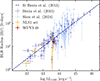 |
Fig. 16. Optical continuum luminosity and Hβ lags for WPVS 48 and other AGN. Included are the data sets of Bentz et al. (2013) (dark blue) and Shen et al. (2024) (light blue) as well as the B-L relation log(RBLR/1lt-day) = 1.527 + 0.533log(λL5100/1044 L⊙) found by Bentz et al. (2013). We also highlight a set of NLS1s: Mrk 110 (Kollatschny et al. 2001; Kollatschny 2003a), Mrk 335 (Grier et al. 2012), NGC 4051 (Denney et al. 2009; Fausnaugh et al. 2017), NGC 4748 (Bentz et al. 2009, 2010), SDSS J113913.91+335551 (Rafter et al. 2013), Ark 564 (Shapovalova et al. 2012), and PG 0934+013 (Park et al. 2017) in orange. |
WPVS 48 is similar in terms of BLR size, luminosity, and derived BH mass to the NLS1 galaxies Mrk 110, Mrk 335, PG 0934+013 and SDSS J113913.91+335551. The optical luminosities and the BLR radii of the sample of reverberation-mapped NLS1 galaxies fall between the lower end and the middle of the R-L range of the AGN samples of Bentz et al. (2013) and Shen et al. (2024). The optical variability amplitude of 1.37 in WPVS 48 is similar to typical variability amplitudes observed in other AGN – NLS1 galaxies and broad-line Seyfert galaxies alike. For most AGN, the variability amplitudes range from ∼1.2 to ∼2 (e.g. Peterson et al. 1998; Bentz et al. 2009; Grier et al. 2012).
WPVS 48 furthermore has some of the same spectral and variability features as the other NLS1s for which optical mean and rms spectra are published: Fe II emission is present in the mean spectra of WPVS 48, Mrk 110 (Kollatschny et al. 2001, see their Fig. 5), Mrk 335 (Grier et al. 2012, see their Fig. 1), NGC 4748 (Bentz et al. 2010, see their Fig. 7), and NGC 4051 (Fausnaugh et al. 2017, see their Fig. 4); however, Fe II seems to be absent or very weak in the corresponding rms spectra (see the same figures except for Mrk 110, there see Fig. 7), which indicates low variability in the Fe II lines. Moreover, we identified several low-intensity He I lines in both the mean and rms spectrum of WPVS 48, as was done in Mrk 110.
5. Conclusions
We performed reverberation mapping of both continuum and emission lines in WPVS 48, using the SALT 10 m telescope. In conclusion, our key findings can be summarised as follows:
-
The BLR of WPVS 48 is stratified with respect to the distance of the line emitting regions. The integrated emission line intensities of Hα, Hβ, Hγ, and He Iλ5876 originate at distances of
 , 15.0
 ,
,  , and
, and  light-days with respect to the optical continuum at 5100 Å. The He IIλ4686 lag of ≲5 days is not perfectly resolved with the minimum sampling of 5 days.
 -
WPVS 48 shows variability similar to other NLS1s and varied by a factor of ∼1.4 in the optical continuum, by a factor of ∼1.2 in the Balmer lines, by a factor of ∼1.4 in He Iλ5876, and by a factor of ∼1.7 in He IIλ4686. The variability amplitudes of the integrated emission lines decrease in the stratified BLR of WPVS 48 with distance to the ionising continuum source. The Balmer decrement in WPVS 48 furthermore increases as a function of decreasing continuum luminosity.
-
We identify variable emission of the Bowen line N IIIλ4640 in the mean and rms spectrum of WPVS 48.
-
We derive interband continuum lags increasing with wavelength in WPVS 48. Assuming two continuum components, we obtain coherent lags of ∼15 days for the secondary component. We therefore suggest a continuum source that is co-located with the Balmer-emitting region.
-
We derive a central BH mass of
 and an Eddington ratio of L/LEdd ≈ 0.39 based on the lag as well as the width of the Hβ rms profile. We address a potential bias due to the presence of a narrow-line Hβ residuum. This narrow-line residuum, however, is not conspicuous in the rms profile. Furthermore, we discussed the correction for a near face-on geometry as suggested by Sobrino Figaredo et al. (2018).
To date, very few NLS1 galaxies have been the subject of a detailed analysis by means of reverberation mapping campaigns. We now have contributed key parameters of the BLR for one specimen of this AGN class.
Acknowledgments
The authors greatly acknowledge support by the DFG grants KO 857/35-1 and KO 857/35-2. MWO gratefully acknowledges the support German Aerospace Center (DLR) within the framework of the ‘Verbundforschung Astronomie und Astrophysik’ through grant 50OR2305 with funds from the German Federal Ministry for Economic Affairs and Climate Action (BMWK). The spectra reported in this paper were obtained with the Southern African Large Telescope (SALT under proposal code 2013-2-GU-001, PI: Kollatschny).
References
- Antonucci, R. R. J. 2023, Galaxies, 11, 102 [NASA ADS] [CrossRef] [Google Scholar]
- Bentz, M. C., Walsh, J. L., Barth, A. J., et al. 2009, ApJ, 705, 199 [NASA ADS] [CrossRef] [Google Scholar]
- Bentz, M. C., Walsh, J. L., Barth, A. J., et al. 2010, ApJ, 716, 993 [Google Scholar]
- Bentz, M. C., Denney, K. D., Grier, C. J., et al. 2013, ApJ, 767, 149 [Google Scholar]
- Blaes, O. M., Davis, S. W., Hirose, S., Krolik, J. H., & Stone, J. M. 2006, ApJ, 645, 1402 [Google Scholar]
- Blandford, R. D., & McKee, C. F. 1982, ApJ, 255, 419 [Google Scholar]
- Boroson, T. A. 2002, ApJ, 565, 78 [NASA ADS] [CrossRef] [Google Scholar]
- Brown, J. S., Holoien, T. W. S., Auchettl, K., et al. 2017, MNRAS, 466, 4904 [Google Scholar]
- Brown, J. S., Kochanek, C. S., Holoien, T. W. S., et al. 2018, MNRAS, 473, 1130 [NASA ADS] [CrossRef] [Google Scholar]
- Cackett, E. M., Chiang, C.-Y., McHardy, I., et al. 2018, ApJ, 857, 53 [NASA ADS] [CrossRef] [Google Scholar]
- Cackett, E. M., Bentz, M. C., & Kara, E. 2021, iScience, 24, 102557 [NASA ADS] [CrossRef] [Google Scholar]
- Cardelli, J. A., Clayton, G. C., & Mathis, J. S. 1989, ApJ, 345, 245 [Google Scholar]
- Chelouche, D., & Zucker, S. 2013, ApJ, 769, 124 [NASA ADS] [CrossRef] [Google Scholar]
- Chelouche, D., Shemmer, O., Cotlier, G. I., Barth, A. J., & Rafter, S. E. 2014, ApJ, 785, 140 [Google Scholar]
- Chelouche, D., Pozo Nuñez, F., & Kaspi, S. 2019, Nat. Astron., 3, 251 [NASA ADS] [CrossRef] [Google Scholar]
- Choloniewski, J. 1981, Acta Astron., 31, 293 [NASA ADS] [Google Scholar]
- Collier, S. J., Horne, K., Kaspi, S., et al. 1998, ApJ, 500, 162 [Google Scholar]
- Davis, S. W., Woo, J.-H., & Blaes, O. M. 2007, ApJ, 668, 682 [NASA ADS] [CrossRef] [Google Scholar]
- Decarli, R., Labita, M., Treves, A., & Falomo, R. 2008, MNRAS, 387, 1237 [NASA ADS] [CrossRef] [Google Scholar]
- Denney, K. D., Watson, L. C., Peterson, B. M., et al. 2009, ApJ, 702, 1353 [NASA ADS] [CrossRef] [Google Scholar]
- Edelson, R., Gelbord, J. M., Horne, K., et al. 2015, ApJ, 806, 129 [NASA ADS] [CrossRef] [Google Scholar]
- Edelson, R., Gelbord, J., Cackett, E., et al. 2019, ApJ, 870, 123 [NASA ADS] [CrossRef] [Google Scholar]
- Edelson, R., Peterson, B. M., Gelbord, J., et al. 2024, ApJ, 973, 152 [Google Scholar]
- Eracleous, M., Livio, M., Halpern, J. P., & Storchi-Bergmann, T. 1995, ApJ, 438, 610 [NASA ADS] [CrossRef] [Google Scholar]
- Fausnaugh, M. M., Denney, K. D., Barth, A. J., et al. 2016, ApJ, 821, 56 [Google Scholar]
- Fausnaugh, M. M., Grier, C. J., Bentz, M. C., et al. 2017, ApJ, 840, 97 [NASA ADS] [CrossRef] [Google Scholar]
- Frank, J., King, A., & Raine, D. J. 2002, Accretion Power in Astrophysics: Third Edition (Cambridge, UK: Cambridge University Press) [Google Scholar]
- Fromerth, M. J., & Melia, F. 2000, ApJ, 533, 172 [NASA ADS] [CrossRef] [Google Scholar]
- Gaskell, C. M., & Peterson, B. M. 1987, ApJS, 65, 1 [NASA ADS] [CrossRef] [Google Scholar]
- Gaskell, M., Thakur, N., Tian, B., & Saravanan, A. 2022, Astron. Nachr., 343, e210112 [NASA ADS] [CrossRef] [Google Scholar]
- Gezari, S., Chornock, R., Lawrence, A., et al. 2015, ApJ, 815, L5 [NASA ADS] [CrossRef] [Google Scholar]
- Goad, M. R., Korista, K. T., & Ruff, A. J. 2012, MNRAS, 426, 3086 [Google Scholar]
- Goodrich, R. W. 1989, ApJ, 342, 224 [Google Scholar]
- Graham, A. W., Onken, C. A., Athanassoula, E., & Combes, F. 2011, MNRAS, 412, 2211 [NASA ADS] [CrossRef] [Google Scholar]
- Grier, C. J., Peterson, B. M., Pogge, R. W., et al. 2012, ApJ, 755, 60 [NASA ADS] [CrossRef] [Google Scholar]
- Grier, C. J., Martini, P., Watson, L. C., et al. 2013a, ApJ, 773, 90 [CrossRef] [Google Scholar]
- Grier, C. J., Peterson, B. M., Horne, K., et al. 2013b, ApJ, 764, 47 [NASA ADS] [CrossRef] [Google Scholar]
- Grupe, D. 2004, AJ, 127, 1799 [NASA ADS] [CrossRef] [Google Scholar]
- Haas, M., Chini, R., Ramolla, M., et al. 2011, A&A, 535, A73 [NASA ADS] [CrossRef] [EDP Sciences] [Google Scholar]
- Hernández Santisteban, J. V., Edelson, R., Horne, K., et al. 2020, MNRAS, 498, 5399 [CrossRef] [Google Scholar]
- Kara, E., Mehdipour, M., Kriss, G. A., et al. 2021, ApJ, 922, 151 [NASA ADS] [CrossRef] [Google Scholar]
- Kishimoto, M., Antonucci, R., Blaes, O., et al. 2008, Nature, 454, 492 [NASA ADS] [CrossRef] [Google Scholar]
- Kobulnicky, H. A., Nordsieck, K. H., Burgh, E. B., et al. 2003, in Instrument Design and Performance for Optical/Infrared Ground-based Telescopes, eds. M. Iye, & A. F. M. Moorwood, SPIE Conf. Ser., 4841, 1634 [Google Scholar]
- Kollatschny, W. 2003a, A&A, 407, 461 [CrossRef] [EDP Sciences] [Google Scholar]
- Kollatschny, W. 2003b, A&A, 412, L61 [NASA ADS] [CrossRef] [EDP Sciences] [Google Scholar]
- Kollatschny, W., & Zetzl, M. 2011, Nature, 470, 366 [NASA ADS] [CrossRef] [Google Scholar]
- Kollatschny, W., & Zetzl, M. 2013, A&A, 549, A100 [NASA ADS] [CrossRef] [EDP Sciences] [Google Scholar]
- Kollatschny, W., Bischoff, K., & Dietrich, M. 2000, A&A, 361, 901 [NASA ADS] [Google Scholar]
- Kollatschny, W., Bischoff, K., Robinson, E. L., Welsh, W. F., & Hill, G. J. 2001, A&A, 379, 125 [NASA ADS] [CrossRef] [EDP Sciences] [Google Scholar]
- Kollatschny, W., Ulbrich, K., Zetzl, M., Kaspi, S., & Haas, M. 2014, A&A, 566, A106 [NASA ADS] [CrossRef] [EDP Sciences] [Google Scholar]
- Kollatschny, W., Ochmann, M. W., Zetzl, M., et al. 2018, A&A, 619, A168 [NASA ADS] [CrossRef] [EDP Sciences] [Google Scholar]
- Kollatschny, W., Ochmann, M. W., Kaspi, S., et al. 2022, A&A, 657, A122 [NASA ADS] [CrossRef] [EDP Sciences] [Google Scholar]
- Korista, K. T., & Goad, M. R. 2001, ApJ, 553, 695 [Google Scholar]
- Korista, K. T., & Goad, M. R. 2004, ApJ, 606, 749 [NASA ADS] [CrossRef] [Google Scholar]
- Kovačević, J., Popović, L. Č., & Dimitrijević, M. S. 2010, ApJS, 189, 15 [Google Scholar]
- Krolik, J. H. 2001, ApJ, 551, 72 [NASA ADS] [CrossRef] [Google Scholar]
- Labita, M., Treves, A., Falomo, R., & Uslenghi, M. 2006, MNRAS, 373, 551 [Google Scholar]
- Liu, C., Gebhardt, K., Cooper, E. M., et al. 2022, ApJS, 261, 24 [NASA ADS] [CrossRef] [Google Scholar]
- Makrygianni, L., Trakhtenbrot, B., Arcavi, I., et al. 2023, ApJ, 953, 32 [NASA ADS] [CrossRef] [Google Scholar]
- McHardy, I. M., Connolly, S. D., Horne, K., et al. 2018, MNRAS, 480, 2881 [NASA ADS] [CrossRef] [Google Scholar]
- Mullaney, J. R., Alexander, D. M., Fine, S., et al. 2013, MNRAS, 433, 622 [Google Scholar]
- Netzer, H. 2019, MNRAS, 488, 5185 [NASA ADS] [CrossRef] [Google Scholar]
- Netzer, H. 2022, MNRAS, 509, 2637 [NASA ADS] [Google Scholar]
- Netzer, H., Elitzur, M., & Ferland, G. J. 1985, ApJ, 299, 752 [Google Scholar]
- Ochmann, M. W., Kollatschny, W., Probst, M. A., et al. 2024, A&A, 686, A17 [NASA ADS] [CrossRef] [EDP Sciences] [Google Scholar]
- Oh, K., Koss, M. J., Ueda, Y., et al. 2022, ApJS, 261, 4 [NASA ADS] [CrossRef] [Google Scholar]
- Onken, C. A., Ferrarese, L., Merritt, D., et al. 2004, ApJ, 615, 645 [Google Scholar]
- Osterbrock, D. E., & Cohen, R. D. 1982, ApJ, 261, 64 [Google Scholar]
- Osterbrock, D. E., & Pogge, R. W. 1985, ApJ, 297, 166 [Google Scholar]
- Park, S., Woo, J.-H., Romero-Colmenero, E., et al. 2017, ApJ, 847, 125 [NASA ADS] [CrossRef] [Google Scholar]
- Park, D., Barth, A. J., Ho, L. C., & Laor, A. 2022, ApJS, 258, 38 [NASA ADS] [CrossRef] [Google Scholar]
- Pei, L., Fausnaugh, M. M., Barth, A. J., et al. 2017, ApJ, 837, 131 [NASA ADS] [CrossRef] [Google Scholar]
- Peterson, B. M., Wanders, I., Bertram, R., et al. 1998, ApJ, 501, 82 [NASA ADS] [CrossRef] [Google Scholar]
- Peterson, B. M., Berlind, P., Bertram, R., et al. 2002, ApJ, 581, 197 [NASA ADS] [CrossRef] [Google Scholar]
- Peterson, B. M., Ferrarese, L., Gilbert, K. M., et al. 2004, ApJ, 613, 682 [Google Scholar]
- Planck Collaboration VI. 2020, A&A, 641, A6 [NASA ADS] [CrossRef] [EDP Sciences] [Google Scholar]
- Rafter, S. E., Kaspi, S., Chelouche, D., et al. 2013, ApJ, 773, 24 [NASA ADS] [CrossRef] [Google Scholar]
- Rodríguez-Pascual, P. M., Alloin, D., Clavel, J., et al. 1997, ApJS, 110, 9 [CrossRef] [Google Scholar]
- Sakata, Y., Minezaki, T., Yoshii, Y., et al. 2010, ApJ, 711, 461 [NASA ADS] [CrossRef] [Google Scholar]
- Schlafly, E. F., & Finkbeiner, D. P. 2011, ApJ, 737, 103 [Google Scholar]
- Shakura, N. I., & Sunyaev, R. A. 1973, A&A, 24, 337 [NASA ADS] [Google Scholar]
- Shapovalova, A. I., Popović, L. Č., Burenkov, A. N., et al. 2010, A&A, 517, A42 [NASA ADS] [CrossRef] [EDP Sciences] [Google Scholar]
- Shapovalova, A. I., Popović, L. Č., Burenkov, A. N., et al. 2012, ApJS, 202, 10 [NASA ADS] [CrossRef] [Google Scholar]
- Shen, Y., Grier, C. J., Horne, K., et al. 2024, ApJS, 272, 26 [NASA ADS] [CrossRef] [Google Scholar]
- Sobrino Figaredo, C., Nuñez, F. P., Ramolla, M., et al. 2018, Revisiting Narrow-Line Seyfert 1 Galaxies and their Place in the Universe, 57 [Google Scholar]
- Sobrino Figaredo, C., Chelouche, D., Haas, M., et al. 2025, ApJS, 276, 48 [Google Scholar]
- Trakhtenbrot, B., Arcavi, I., Ricci, C., et al. 2019, Nat. Astron., 3, 242 [Google Scholar]
- Véron-Cetty, M. P., Véron, P., & Gonçalves, A. C. 2001, A&A, 372, 730 [NASA ADS] [CrossRef] [EDP Sciences] [Google Scholar]
- Vestergaard, M., & Peterson, B. M. 2006, ApJ, 641, 689 [Google Scholar]
- Vincentelli, F. M., McHardy, I., Cackett, E. M., et al. 2021, MNRAS, 504, 4337 [CrossRef] [Google Scholar]
- Winkler, H. 1997, MNRAS, 292, 273 [Google Scholar]
- Winkler, H., Glass, I. S., van Wyk, F., et al. 1992, MNRAS, 257, 659 [NASA ADS] [Google Scholar]
- Wright, E. L. 2006, PASP, 118, 1711 [NASA ADS] [CrossRef] [Google Scholar]
- Xu, D., Komossa, S., Zhou, H., et al. 2012, AJ, 143, 83 [NASA ADS] [CrossRef] [Google Scholar]
- Zhou, S., Sun, M., Feng, H.-C., et al. 2025, ApJ, 986, 137 [Google Scholar]
- Zucker, S., & Mazeh, T. 1994, ApJ, 420, 806 [NASA ADS] [CrossRef] [Google Scholar]
We are able to perform this improvement as Fe IIλ4233 is not variable in WPVS 48. This is shown in the rms spectrum (see Fig. 2), which shows no variability in any Fe II line. In general, Fe II lines can be variable (e.g. Gaskell et al. 2022).
The presented mean and rms spectra are a combination of the blue and red intercalibrations merged at 5645 Å.
We note a [O III] λ5007 residual comparable in height to the profile of Hβ in the rms spectrum. This high residual is produced by the skewed [O III] λ5007 profile in spectrum 15 (from 2014-03-28) likely caused by poor seeing conditions. If spectrum 15 is omitted, the [O III] λ5007 residual is smaller by the factor of ∼2, whereas the rms profiles of the broad emission lines are not affected.
The formalism in Chelouche & Zucker (2013) includes a lag τpri for the primary component as well. However, the formalism was simplified in later studies (e.g. Chelouche et al. 2019; Sobrino Figaredo et al. 2025) assuming a small τpri compared to both the lag of the secondary component τsec and the sampling.
NGC 5548 exceeded the upper limit of the given range with a lag of ∼5.9 days between hard X-rays (1.5–10 keV) and the V band (Edelson et al. 2019).
Ochmann et al. (2024) measured a FWHM of ∼2200 km s−1 for Hβ in NGC 1566. While exhibiting relatively narrow BLR lines, NGC 1566 formally is not a NLS1.
Appendix A: Additional figures
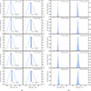 |
Fig. A.1. Left panel: CCFs of the interband continuum correlations with respect to the continuum light curve at 4265 Å (a). The time lag, τcent, is denoted by a dashed line; the shaded area corresponds to a ±1σ interval. Right panel: Cross-correlation centroid distributions after 20,000 runs employing FR and RSS of the various continua with respect to the combined continuum at 4265 Å (b). |
Appendix B: Additional tables
Continuum Flux Densities.
Line Fluxes.
All Tables
Log of spectroscopic observations of WPVS 48 throughout the reverberation mapping campaign from late 2013 to mid-2014.
Continuum boundaries and line integration limits (2) as well as the sections used to fit the pseudo-continua (3).
Extinction-corrected B, V, and R values for the combined host galaxy plus AGN fluxes, and for the host galaxy and AGN fluxes alone, as determined by the FVG method.
Variability statistics of the investigated continua and emission lines with minimum (2) and maximum flux density or integrated flux (3), peak-to-peak ratio (4), mean flux density (5), standard deviation (6), and fractional variation (7).
Interband cross-correlation lags τ with respect to the continuum at 4265 Å (at 4425 Å in observed frame) as well as the maximum correlation coefficient rmax and the fractional contribution α of the secondary component, respectively, for the univariate and bivariate model.
Cross-correlation lags of the continuum light curves at 4265 Å and 5100 Å (at 4425 Å and 5290 Å in observed frame, respectively) with the light curves of the integrated lines.
FWHM and line dispersion σline of the mean and rms profiles of the Balmer lines and He Iλ5876.
Inferred velocities of (projected) rotational and turbulent motion as well as scale height of the prominent emission lines.
Key parameters of NLS1 galaxies with existing reverberation mapping data: Flux density (2) and variability amplitude (3) of the continuum at 5100 Å, optical luminosity (4), FWHM of the rms profile of Hβ (5), Hβ lag to the optical continuum (6), BH mass (7) and Eddington luminosity (8).
All Figures
|
Fig. 1. Top panel: Reduced optical spectra of WPVS 48 during the variability campaign from December 2013 to June 2014. The spectra were calibrated to the same absolute [O III] λ5007 flux of 244 × 10−15 erg cm−2 s−1. The identified emission features are labelled. Bottom panel: Zoomed-in image of the continuum and the low-intensity emission lines. The conspicuous feature at ∼5490 Å is a residual from night-sky emission. |
| In the text | |
|
Fig. 2. Combined mean spectrum (black) and rms spectrum (red) of WPVS 48 from our campaign. The partition in the two intercalibrations (see Sect. 2 for details) is shown with a grey dashed line. The rms spectrum was scaled to allow for a direct comparison. The analysed continuum regions and the identical pseudo-continua used for linear continuum subtraction are highlighted with blue bars below the spectra. The line integration limits are marked by the shaded areas. All emission lines of He I are displayed in orange. |
| In the text | |
|
Fig. 3. Extinction corrected B-V flux variations. The blue dashed line represents the best linear fit of the AGN slope of WPVS 48 and the red shaded area the host slopes of nearby AGN. |
| In the text | |
|
Fig. 4. Extinction corrected B-R flux variations. The blue dashed line represents the best linear fit of the AGN slope of WPVS 48 and the red shaded area the host slopes of nearby AGN. |
| In the text | |
|
Fig. 5. Detailed emission line identification in the mean spectrum close to He IIλ4686. We identify N IIIλ4640 and C IVλ4658 (Osterbrock & Cohen 1982) and further labelled the position of the Fe II (37, 38) emission bands (for a template of Fe II, see Park et al. 2022) as well as [Ar IV] λλ4712, 4740. |
| In the text | |
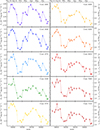 |
Fig. 6. Optical continuum light curves measured within the integration limits given in Table 2. |
| In the text | |
|
Fig. 7. Mean centroid lags τcent according to the univariate model (blue squares) as well as centroid lags τsec (blue circles) and fractional contribution α (red circles) of the secondary component according to the bivariate model (Chelouche et al. 2019) as a function of the effective wavelength of the continuum. We include the univariate lags of photometric light curves published by Sobrino Figaredo et al. (2018) as grey squares. We note that Hβ contributes to the flux in the V band. The lags and the fractional contribution are measured with respect to the continuum at 4265 Å as a function of the effective wavelength of the continuum. The colouring of the shaded background corresponds to the light curves in Fig. 6. The errors correspond to the 68% (±1σ) confidence level after a Monte-Carlo simulation with 20 000 runs. The data of τsec and α have been slightly shifted in wavelength for better readability. |
| In the text | |
|
Fig. 8. Emission line light curves of the Balmer lines as well as He Iλ5876 and He II λ4686 measured within the integration limits given in Table 2. The continuum light curve at 5100 Å is included for reference. |
| In the text | |
|
Fig. 9. Left panels: CCFs of the integrated Balmer lines in blue, the integrated He I λ5876 line in orange and the integrated He II λ4686 line in red, with respect to the continuum light curve at 5100 Å. The time lag, τcent, is denoted by a dashed line; the shaded area corresponds to a ±1σ interval from the Monte-Carlo simulations. Right panels: Cross-correlation centroid distributions after 20 000 runs employing FR and RSS of the integrated Balmer lines in blue, the integrated He I λ5876 line in orange and the integrated He II λ4686 line in red, with respect to the continuum at 5100 Å. |
| In the text | |
|
Fig. 10. Normalised mean (black) and rms (red) line profiles of the Balmer and the prominent He Iλ5876 and He IIλ4686 emission lines. While the mean profiles corrected for contributions of narrow forbidden lines are shown in red, the grey dashed line indicates the uncorrected mean profiles of Hα and Hγ. We note that the blue wing of the mean He IIλ4686 profile blends with emission from N IIIλ4640, C IVλ4658, and Fe II (37, 38) multiplets. |
| In the text | |
|
Fig. 11. Top panels: Comparison of the normalised mean (left panel) and rms (right panel) line shapes of the Balmer emission lines with the He Iλ5876 emission line. Bottom panels: Comparison of the normalised mean (left panel) and rms (right panel) line shapes of the He Iλ5876 emission line with the He IIλ4686 emission line. We note that the blue wing of the mean He IIλ4686 profile blends with emission from N IIIλ4640, C IVλ4658, and Fe II (37, 38) multiplets. |
| In the text | |
|
Fig. 12. Comparison of the spectroscopic continuum light curve at 6810 Å and the photometric R band light curve from Sobrino Figaredo et al. (2018) (effective wavelength in the rest frame of WPVS 48 λeff = 6750 Å), shifted by −1.57 × 10⁻¹⁵ erg cm−2 s−1 Å−1. |
| In the text | |
|
Fig. 13. The rms spectrum of the SALT campaign corrected for Galactic foreground extinction (red). Two power-law models are fitted to the continuum slope. The first considers only the continua at 5100 Å and bluewards giving a spectral index β = 2.61 ± 0.06 (black); the second considers all measured continua giving a spectral index β = 1.82 ± 0.03 (grey). |
| In the text | |
|
Fig. 14. Balmer decrement, F(Hα)/F(Hβ), of the broad-line components vs continuum intensity at 5100 Å. The dashed line on the graph represents the linear regression. |
| In the text | |
|
Fig. 15. Balmer decrement, F(Hα)/F(Hβ), of the broad-line components vs broad-line Hβ intensity. The dashed line on the graph represents the linear regression. |
| In the text | |
|
Fig. 16. Optical continuum luminosity and Hβ lags for WPVS 48 and other AGN. Included are the data sets of Bentz et al. (2013) (dark blue) and Shen et al. (2024) (light blue) as well as the B-L relation log(RBLR/1lt-day) = 1.527 + 0.533log(λL5100/1044 L⊙) found by Bentz et al. (2013). We also highlight a set of NLS1s: Mrk 110 (Kollatschny et al. 2001; Kollatschny 2003a), Mrk 335 (Grier et al. 2012), NGC 4051 (Denney et al. 2009; Fausnaugh et al. 2017), NGC 4748 (Bentz et al. 2009, 2010), SDSS J113913.91+335551 (Rafter et al. 2013), Ark 564 (Shapovalova et al. 2012), and PG 0934+013 (Park et al. 2017) in orange. |
| In the text | |
|
Fig. A.1. Left panel: CCFs of the interband continuum correlations with respect to the continuum light curve at 4265 Å (a). The time lag, τcent, is denoted by a dashed line; the shaded area corresponds to a ±1σ interval. Right panel: Cross-correlation centroid distributions after 20,000 runs employing FR and RSS of the various continua with respect to the combined continuum at 4265 Å (b). |
| In the text | |
Current usage metrics show cumulative count of Article Views (full-text article views including HTML views, PDF and ePub downloads, according to the available data) and Abstracts Views on Vision4Press platform.
Data correspond to usage on the plateform after 2015. The current usage metrics is available 48-96 hours after online publication and is updated daily on week days.
Initial download of the metrics may take a while.