| Issue |
A&A
Volume 706, February 2026
|
|
|---|---|---|
| Article Number | A160 | |
| Number of page(s) | 17 | |
| Section | Astrophysical processes | |
| DOI | https://doi.org/10.1051/0004-6361/202555190 | |
| Published online | 06 February 2026 | |
Main and inter-pulse interaction in PSRs J1842+0358 and J1926+0737: evidence of inter-pole communication
1
ASTRON, the Netherlands Institute for Radio Astronomy Oude Hoogeveensedijk 4 7991 PD Dwingeloo, The Netherlands
2
Jodrell Bank Centre for Astrophysics, Department of Physics and Astronomy, The University of Manchester Manchester M13 9PL, UK
★ Corresponding author: This email address is being protected from spambots. You need JavaScript enabled to view it.
Received:
17
April
2025
Accepted:
30
November
2025
Abstract
Our understanding of the elusive radio-pulsar emission mechanism would be deepened by determining the locality of the emission. Pulsars in which the two poles interact might help us to solve this challenge. We report the discovery of interacting emission between the main and the inter-pulse in two pulsars, J1842+0358 and J1926+0737, based on FAST and MeerKAT data. When the emission is bright in one pulse, it is dim in the other. Even when split into just two groups (strong versus weak), the anti-correlated brightness can change by a factor of ≳2. Both sources furthermore show the same quasi-periodic modulation from the main and inter-pulse at timescales exceeding 100 pulse periods. The longitude stationary modulation from at least one pulse suggests that it is a key signature for inter-pulse pulsars with a main and inter-pulse interaction. If the interaction occurs within an isolated magnetosphere without external influences, either communication between the opposite poles is required, or global changes drive both. This detailed study of these two sources was only made possible by an improved sensitivity. The fact that both show two-pole modulation strongly suggests that this is a general phenomenon in inter-pulse pulsars. In regular pulsars, only one pole is visible, and a number of these regular pulsars show correlated changes between the profile and the spin-down rate that are also thought to be caused by global magnetospheric changes. Our results strengthen the case that these interactive magnetospheres are common to all pulsars.
Key words: pulsars: individual: J1842+0358 / pulsars: individual: J1926+0737
© The Authors 2026
 Open Access article, published by EDP Sciences, under the terms of the Creative Commons Attribution License (https://creativecommons.org/licenses/by/4.0), which permits unrestricted use, distribution, and reproduction in any medium, provided the original work is properly cited.
This article is published in open access under the Subscribe to Open model. This email address is being protected from spambots. You need JavaScript enabled to view it. to support open access publication.
1. Introduction
The individual pulses emitted by radio pulsars are highly variable. While this diversity is stochastic, some pulsars show systematic patterns as well. Sub-pulses (pulses that are narrower than the average profile) might, for example, drift in longitude or display modulated periodic intensity, without phase variations. Both types are relatively common (see sub-pulse surveys by e.g. Rankin 1986; Weltevrede et al. 2006, 2007; Basu et al. 2016, 2019, 2020; Song et al. 2023) and are related to the fundamental magnetospheric radio emission. Ruderman & Sutherland (1975) theorised that this emission originates from localised discrete sub-beams that rotate around the magnetic axis. While this provides a simple model for understanding emission beams, there are challenges both theoretically (e.g. Chernoglazov et al. 2024) and observationally (e.g. Wang et al. 2025). The study of single-pulse properties thus provides useful constraints on the magnetospheric emission mechanisms.
Inter-pulse pulsars, in which two pulses are seen per period, usually half a stellar rotation apart, are especially interesting in this context. Only ∼3% of the population are inter-pulse pulsars (Maciesiak et al. 2011), but they offer valuable insights into the magnetospheric structure because the main pulse (MP) and inter-pulse (IP) are generally interpreted as emission from the two opposite poles. These pulsars therefore possess a specific geometry in which the magnetic and rotation axes are nearly perpendicular to each other: an orthogonal rotator. As one of the necessary simplifications in the Ruderman & Sutherland (1975) model is the assumption of an aligned rotator (where magnetic and rotation axes coincide), it is interesting to study how emission is affected in this opposite case, the orthogonal rotator. Moreover, it might next be wondered whether and how emission from the two poles is related, and this can also only be investigated in an inter-pulse pulsar.
Ample evidence suggests that these pulses that are seen half a period apart originate from both poles and not from two regions on a single pole from an aligned rotator. The polarisation position angles (PAs), for example, for MP and IP can both be fitted using the rotation vector model (RVM; Radhakrishnan & Cooke 1969), with a single underlying opposite-pole geometry (cf. PSR B0906−49, Kramer & Johnston 2008). In PSR J1906+0746 (van Leeuwen et al. 2015), geodetic precession allowed for a measurement of the changes in the PAs of both poles because our line of sight (LoS) evolves and even crossed one pole (Desvignes et al. 2019). Further evidence is provided by the unchanging separation between MP and IP at various observing frequencies. In single-pole emission, the components generally separate more at lower frequencies. For PSR B1702−19, for example, Biggs et al. (1988) showed that the MP-IP peak separation remained 180° from 408 to 1420 MHz. Finally, the MP and IP average profiles are usually very narrow compared to their separation. In contrast, broad pulse widths and bridge emission more often occur in single-pole pulsars (as in, for example, PSR B1929+10; Rankin & Rathnasree 1997; Kou et al. 2021).
Some inter-pulse pulsars exhibit an interesting and surprising phenomenon: Their MP and IP emission is correlated, which is evidence of communication between the two poles. This was first discovered in PSR B1822−09 (Fowler & Wright 1982) with detailed follow-up by Gil et al. (1994). In PSRs B1702−19 (Weltevrede et al. 2007), B1055−52 (Biggs 1990; Weltevrede et al. 2012), B1822−09 (Backus et al. 2010; Yan et al. 2019), B1929+10 (Kou et al. 2021), and B0823+26 (Chen et al. 2023), the correlation is furthermore associated with an intensity modulation of the same periodicity in the MP and IP. Intriguingly, these periodic variations are phase-locked over many thousands of pulse periods. Sources can also exhibit a phase delay between MP and IP. These properties are not easily explained by existing pulsar models. For emission from different poles, even the Ruderman & Sutherland (1975) order-of-magnitude model does not explain these strictly identical configurations and periodicities. In addition, van Leeuwen & Timokhin (2012) showed that when derived exactly, the modulation depends strongly on the local configuration of each pole.
This adds to the interest in the fact that the two poles must be connected in some way; and this is not possible through the traditionally defined open-field line regions in which radio emission is generated (e.g. see discussions in Weltevrede & Wright 2009). Although a single-pole model would explain the phase locking and identical periodicities, the above-mentioned geometric evidence still favours a two-pole emission.
Our understanding of the inter-pulse pulsar population would be improved if we determined whether MP-IP phase locking is standard, or is special in some way. The Thousand-Pulsar-Array (TPA) programme (Johnston et al. 2020) covered over 30 inter-pulse pulsars at L band using the full MeerKAT array and observed more than 1000 pulses at least once. Their sub-pulse modulation properties were studied by Song et al. (2023). Even at the MeerKAT sensitivity, however, the modulation and correlation could not always be detected when the dimmest inter-pulse was too weak. We thus carried out a campaign using FAST (Five-hundred-meter Aperture Spherical Telescope, Nan et al. 2011), with a higher sensitivity and longer single-pulse sequences.
We report that two more inter-pulse pulsars, PSRs J1842+0358 and J1926+0737, show correlated quasi-periodic emission from the MP and the IP. We base this on data from MeerKAT and FAST. The two pulsars were discovered in the Parkes Multibeam Pulsar Survey (Lorimer et al. 2006; Eatough et al. 2010) and inhabit the young to middle part of the P−Ṗ diagram. PSRs J1842+0358 and J1926+0737 have short spin periods of around 0.23 s and 0.32 s, with a spin-down rate Ṗ of 8.1E−16 s/s and 3.8E−16 s/s, respectively. The inferred spin-down luminosities are 2.5E33 erg/s and 4.6E32 erg/s, with characteristic ages of 4.6E6 yr and 1.3E7 yr. For both pulsars, the MP and IP emissions were thought to originate from two opposite poles by Maciesiak et al. (2011, and references therein), but no polarisation data were presented.
The structure of our paper is as follows: The MeerKAT and FAST observations are described in Sect. 2, the single-pulse analysis of PSRs J1842+0358 and J1926+0737 is described in Sects. 3 and 4, where the correlations in the MP and the IP emission are established, with the identified quasi-periodic modulations. Finally, we present our discussions and conclusions.
2. Observations
2.1. MeerKAT
The MeerKAT pulse stacks were taken from the TPA single-pulse pipeline. A full description of the production of these single-pulse stacks is given by Song et al. (2023). There was a single observation for each of PSRs J1842+0358 and J1926+0737, covering 2343 and 4612 single pulses, respectively. The observations were centred at about 1284 MHz, with a bandwidth of 856 MHz. The data were polarisation calibrated but not flux calibrated. The on-pulse regions were automatically identified and a straight-line-fit to the off-pulse region was subtracted from each single pulse to produce the baseline-subtracted single-pulse stack.
2.2. FAST
The FAST observations used the Swift Calibration mode, with a 49.152 μs sampling time and 4096 frequency channels. The observations were centred at 1250 MHz with a bandwidth of 500 MHz (Jiang et al. 2019). Based on noise diode injection at the start of each observation, the data were calibrated for polarisation (but not flux density). The raw data were first passed to DSPSR to produce single pulses with 1024 phase bins using the MeerKAT ephemerides. The original frequency resolution of 4098 channels was reduced to 512 for further processing. The same set of frequency channels affected by radio frequency interference (RFI) was removed from each single pulse. The data were corrected for Faraday rotation using rotation measure (RM) values derived from the MeerKAT observation for PSR J1842+0358, and determined using RMSYNTH (Weltevrede 2016) for PSR J1926+0737. We focus on single-pulse properties; detailed polarisation properties are presented in Sun et al. (2025). On-pulse regions were identified by eye, and a linear baseline slope was subtracted from each single pulse. The observations of PSRs J1842+0358 and J1926+0737 contained 4849 and 4476 single pulses after processing. For presentation purposes, the single pulses of the FAST data were normalised by the peak intensity of the corresponding average profile.
3. PSR J1842+0358
In this section, we discuss the MeerKAT and FAST data and analysis for PSR J1842+0358. The subsequent sections present the average profile morphology (Sects. 3.2 and 3.3), the single-pulse analysis using average profiles of different intensities (Sect. 3.4), the fluctuation spectra (Sect. 3.5), and the cross-correlation analysis (Sect. 3.6), respectively.
3.1. MeerKAT pulse stack
The TPA observed this pulsar once. No clear periodicity was identified by Song et al. (2023); their two-dimensional fluctuation spectrum (2DFS; Edwards & Stappers 2002) shows a slight increase in power towards the very lowest frequency of the MP, but no clear structure is identified for the IP. The pulse stacks and average pulse profile are presented in Fig. 1. Although the MP (left) shows occasionally brighter and wider pulses (e.g. pulses 400 and 1100), no clear periodicity is identified. The IP is hardly detected, although some pulses appear brighter (e.g. pulses 1200 to 1300). The intensity modulation in MP and IP does motivate further study. To do this, we exploited the higher S/N of the FAST observation, which is presented in the remainder of this section.
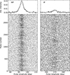 |
Fig. 1. Main pulse (left) and interpulse (right) pulse stacks of PSR J1842+0358 from the MeerKAT observation. The pulse sequences are averaged over ten single pulses, but the pulse number on the y-axis still denotes the single-pulse number. The corresponding average profiles of all single pulses are shown in the top panels. |
3.2. Average pulse-profile morphology
In the average profile of PSR J1842+0358 as detected by FAST (Fig. 2), the MP (left) consists at least two components, with a small component appearing at the trailing edge of the pulse profile (pulse longitude about 92°). Inspecting the single pulses, some have bright and wide emission, especially towards the trailing edge of the pulse profile (e.g. pulse around 200 in Fig. 3a), which also form the additional component in the average profile. The same wider pulses are seen in the MeerKAT observation in Fig. 1. The IP (right) is much weaker than the MP, and has a asymmetric profile. The widths of the MP and the IP at 10% of their peaks, are around 11° and 14°, respectively.
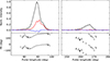 |
Fig. 2. Average pulse profile of PSR J1842+0358 from the FAST data for MP (left) and IP (right). The total intensity profile (normalised by the MP peak) is shown in black, and linear and circular polarisation are plotted in red and blue, respectively. The bottom panels show the PAs of the on-pulse regions. |
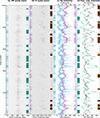 |
Fig. 3. First 1000 single pulses for PSR J1842+0358. Pulse stacks (MP, IP) and intensities (single-pulse, running-averaged). Panel a: Pulse stack of the MP. The blue and green margin bars mark the bright pulses, based on the intensities of the single pulses (blue, left) or their running averages (green, right). Panel b: Same as (a) but for the IP, now with violet and brown for single-pulse or running-averaged intensities, respectively. Panel c: Single-pulse intensities of the MP and the IP, with the running averaged intensities plotted on top. Margin bars are identical to the left of (a) and (b). Panel d: Running averaged intensities of the MP and the IP plotted alone, along with the corresponding selected bars (the same as those on the right of a and b). The rest of the PSR J1842+0358 pulse stacks are available online. |
3.3. Evidence of an orthogonal rotator
Maciesiak et al. (2011) claimed the pulsar is orthogonal, but without a quantitative geometry measurement. Detailed polarisation analysis of the inter-pulse pulsars is presented in Sun et al. (2025); we here focus only on the simple geometric arguments that suggest this pulsar is likely an orthogonal rotator.
The average profiles of the FAST observation are presented in Fig. 2 top panels. The separation between the peak of the MP and the peak of the IP is 177.5°, close to 180° – which is expected for an orthogonal rotator. Further evidence of a double-pole geometry is the lack of emission in between the MP and the IP. The pulse widths at 10% of the peak intensity are of the order of 10° for the MP and the IP, which are both much smaller than the MP-IP separation. This behaviour in the pulse profile is less likely to be produced by a single-pole geometry, whose pulse profiles are relatively wide and tend to include bridge emission. There is no significant evolution across the 500 MHz bandwidths for FAST and MeerKAT, and we are not aware of other relevant (public) data.
Polarisation profiles were computed using PPOL in PSRSALSA1 (Weltevrede 2016) and are shown in Fig. 2. We obtained consist linear/circular polarisation profiles as presented in Sun et al. (2025). The position angles (PAs) were computed from the linear polarisation. According to the RVM model (Radhakrishnan & Cooke 1969), the PAs form an S-shaped curve as the magnetic fields pass the LoS. The PA points for the MP and the IP are shown in the bottom panels of Fig. 2. Although it includes less accurate PA points, the overall shape of the curve in the IP is clear enough. The positive slope of the MP PAs and the negative slope of the IP PAs suggest that the sign of the impact parameter β is different for the MP and IP, with α, the angle between the rotation and the magnetic axis, assumed to be close to 90°. Further discussion of how the slopes of the PA give rise to different LoS cut of the emission beam is in Sect. 5.3.1. In Sun et al. (2025), a polarisation fit indeed suggests that this pulsar is an orthogonal rotator. We note that their fitted PA direction of the IP is the opposite to ours here. The authors themselves pointed out, however, that their result is based on only two PA points and needs clarification through longer observations. From the multiple lines of evidence described above, we conclude PSR J1842+0358 is an orthogonal rotator.
3.4. Single-pulse stack
The most significant feature in the single-pulse stack (the first 1000 pulses shown Figs. 3a and 3b) is that IP and MP display intensity variability, and occasionally produce bright pulses. Especially the IP (panel b) shows significant variations in single-pulse brightness, together with changes in emission phase. One example is found around pulse 800. After a sequence of weak emission, the pulses start from a late pulse longitude of 270° at pulse 785, but after around 35 pulses the pulse is centred around 263°. The pulses next shift towards later pulse longitude for another 30 pulses at around 267° until the emission is too weak to be seen. In the majority of the IP emission blocks, the trailing components appear first and the sub-pulses drift to earlier pulse longitudes. This suggests some form of sub-pulse modulation in the IP, though without a strict periodicity (for a detailed analysis see Sect. 3.5). The timescales of these IP periodicities are long2, of the order of 100 pulses.
In terms of the MP, the bright sub-pulses in the single pulses form a band-like structure (visible, e.g., in Fig. 3a, around pulse 410). This structure is even more visible in the ten single-pulse-averaged MeerKAT observation in Fig. 1. There are some quasi-periodic intensity changes, but without a clear phase modulation. Some pulses show a wider pulse width with additional emission at pulse longitude 92 to 95°, which also results in higher intensities in the single pulses (e.g. around pulse 200, 420 and 620). The timescales of intensity changes seem to be shorter than that presented in the IP. More detailed analysis of the MP single-pulse behaviour is presented in Sect. 3.5.
From the single-pulse stack, the anti-correlation between the MP and the IP is already indicated. For example, around pulse 380 and 600 to 700, the MP is weak while the IP is bright. For pulse 750, the opposite is seen: the MP becomes bright while the IP fades. This anti-correlation is investigated in the remainder of this section, where we describe a more quantitative way of selecting the bright and weak pulses.
3.4.1. Separating bright and weak pulses
These bright and weak pulses can be formally separated through their summed on-pulse intensities. We can next compare the resulting average pulse profiles for each. More interestingly, average profiles can also be constructed when the other component is bright or weak. This is sensitive to the bright and weak anti-correlations suggested by the pulse stack. For PSR J1842+0358, the brightest 1/3 of MP and IP pulses are labelled bright, the remainder, weak. This 1/3-rd boundary best agrees with the by-eye perception of the bright IP pulse cut-off. The bright pulses are indicated by horizontal bars in the left margin of Figs. 3a, b, in blue (MP) and violet (IP). The single-pulse intensities (Fig. 3c) show that bright blocks in the IP are more organised than the MP. The variability in the MP seems more stochastic.
The pulse energy distributions, showing the single-pulse energies normalised by the mean MP intensity (Fig. 4), are continuous for MP and IP. There is no significant bi-modality and thus no evidence of classical mode changing. We suggest, rather, that (quasi-)periodic modulations produce the single-pulse intensity variations (see also Sect. 3.5).
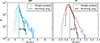 |
Fig. 4. Pulse energy distributions of PSR J1842+0358 for MP (left) and IP (right), with single-pulse energies (blue and violet) and running-averaged pulse energies (green and brown). The same colours of the pulse energies corresponding to the bright groups as in Fig. 3 apply. The weak pulse energy distributions use the same but lighter set of colours. The two pulse energies are normalised by the mean MP energy. The vertical line indicates the cut of the two groups, of 1/3 bright and 2/3 weak pulse intensities (as described in Sect. 3.4.1). |
We next perform the bright and weak separation again, but using running-averaged intensities instead of single pulses. That smooths out stochastic pulse variability (seen in the horizontal bars in Fig. 3c), making the long-term variability becomes more significant. For each pulse number we now use the mean intensity of the 11 pulses around it. These are shown in Fig. 3d in green (MP) and brown (IP)3. Now the quasi-periodic modulations are more pronounced. The resulted pulse energy distributions are in green lines in Fig. 4. The cut-off of the bright and weak pulses is similar to that of the single pulses, at (1/3, 2/3), even though the distributions become narrower. The result is shown in the green and brown bars in the right margin of panels Figs. 3a, b, and in d. These form blocks with more continuity and the MP-IP anti-correlation becomes even more visible in the graph lines and in the block bars.
3.4.2. (Anti-)correlation between the MP and IP brightness
From these bright and weak groups we now construct average pulse profiles, to show whether these profiles have different shapes and/or intensities, and study their possible (anti-)correlation. These profiles are shown in Fig. 5. They indeed demonstrate an anti-correlation between the MP and the IP. In panel a, the MP average pulse profile constructed using the weak group of IP intensities (dark red) has higher intensity than that of the bright group of IP intensity (brown). Similarly in the IP (panel b), the average profile from the MP weak pulses (cyan) is brighter than those constructed from the MP bright pulses (green).
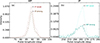 |
Fig. 5. Average pulse profiles of MP and IP of PSR J1842+0358 based on the weakest and strongest groups of running-averaged pulses from the other pulse. Panel a: MP profiles based on, from top to bottom: weakest IP in running averaged (dark red), then brightest IP in running averaged (brown) marked in Fig. 4b. Panel b: IP average pulse profiles of the weakest and brightest groups of the MP, with colours in cyan and green, marked in Fig. 4a. |
The same anti-correlation is revealed by comparing the profiles based on the bright and weak groups of single-pulse intensities (see Figs. A.1c and A.1d and a description of the normalised profiles as well). In addition, the two IP profiles based on the running averaged intensities of the MP show a larger difference in intensity than those based on the single-pulse intensities. This indicates that the stochastic variability in the MP single pulses does not correlate with the changes in the IP intensities – rather, the long-term variability (which is more pronounced in the running averaged intensities) is the reason for the anti-correlation between the MP and the IP. Profiles constructed using only the first and second half of the pulse sequence confirm the anti-correlation.
Longitude-resolved cross-correlation maps between MP and IP independently also report the same anti-correlation (Appendix A.2). These correlation maps show that such anti-correlation is present in both the FAST and MeerKAT observations.
In summary, the averaged pulse profiles constructed using the bright and weak pulses of the other pulse indicate the anti-correlation between the MP and the IP, and this correlation is associated with the long-term variability. In addition, the longitude-resolved correlation map further demonstrates this anti-correlation appears for all on-pulse longitudes between the MP and the IP at zero phase delay, and this correlation is maintained over years. The timescales of the long-term variability in the MP and the IP are investigated next.
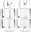 |
Fig. 6. Fluctuation spectra of PSR J1842+0358 for MP (left) and IP (right). Top: Average pulse profile and the modulation index (black dots with error bars) against pulse longitude. Middle: LRFS as fluctuation frequency (1/P3, in cycles per period, cpp). Its side panel shows the integrated power. Bottom: 2DFS, with fluctuation frequencies on both axes in cpp, with 1/P3 vs. 1/P2. Its left and bottom subpanels show the horizontal and vertical integrated power. The orange curve is the horizontal mirror image of the black curve in the bottom panel, indicating whether there are any possible drift in the pulse stack. The greyscale bars indicates the scale. Values above 1 are clipped. |
3.5. Long-term quasi-periodic modulations
Single-pulse periodicities can be identified from the longitude-resolved fluctuation spectrum (LRFS; Backer 1970), while the 2DFS (introduced earlier) can next identify whether the periodicity shows drift or not. They were calculated through fast Fourier transforms (FFTs) on single-pulse blocks of a certain length. Given the long-term intensity variabilities we choose a relatively long block size of 2048 pulses. The overall LRFS or 2DFS is an averaged version of those computed from all blocks (two in this case). The LRFS computes FFTs at each pulse longitude, such that the periodicities (P3) are determined per pulse number for each pulse longitude. The LRFS can also be used to compute the modulation indices, representing the fractional change of the single-pulse intensity for each pulse longitude (black dots in the top panel of Fig. 6, and see Weltevrede et al. 2006 for details on how these are computed).
The modulation for MP and IP traces a U-shaped curve, lowest at the intensity peak and increasing towards the edge. The IP shows high indices of around 2 because its single-pulses change from nearly absent to clearly detectable. The MP single pulses are always detected, and its modulation indices are 1−1.5. This behaviour in the FAST data is consistent with the TPA data.
In the LRFS (second row in Fig. 6), MP and IP display a broad spectral feature at the lowest 1/P3 frequencies, of ∼0.02 cpp and below. They are centred at P3 ≃ 114 ± 40 for the MP and P3 ≃ 112 ± 76 for the IP. This periodicity is more pronounced for the IP. The MP LRFS reveals power along all 1/P3 frequencies for the on-pulse regions, with the integrated 1/P3 curve clearly offset from zero – indicating that the MP exhibits large stochastic variability. Having a closer look of the IP LRFS, the trailing component around 268−270° revealed a shorter periodicity, around 65 P. This mostly relates to the bright trailing edge emission. This is also hinted by a peak in the integrated 1/P3 frequency side panel. Given the quasi-periodicity, this short periodicity is nevertheless blended with the long-term modulation. The frequency features are equally present when halving the sequence.
From the 2DFS of the MP (bottom panel in left column of Fig. 6), the lowest frequency feature is centred around 1/P2 = 0 frequency, which rules out significant drift. In the 2DFS of the IP a negative drift is observed in the bottom integrated 1/P2 panel. Sub-pulses thus drift from the trailing to leading part of the IP. This drift in the trailing part of the IP is visible at, for example, pulse 788−820 and 920−945 in Fig. 3b. We constructed sub-pulse phase tracks that reveals a roughly 180° difference between the MP and the IP, confirming the findings above (Appendix A.4).
In summary, spectral analysis shows that MP and IP possess long-term quasi-periodicities. The MP displays short-term quasi-periodicities as well. The MP modulation is longitude stationary. The IP has a more clearly defined lowest frequency feature and exhibits negative drift.
3.6. Timescales of the correlated emission
As discussed in Sects. 3.4 and 3.5, the MP and the IP have the same long-term quasi-periodic modulations, and these variations are anti-correlated. The periodicity can also be tested using the auto-correlation of the summed pulse intensities. By definition the auto-correlation peaks at zero and is symmetric about zero. In Fig. 7a, the MP auto-correlation (in blue) shows a fast decrease for lags smaller than 10, with some evidence of an increase at around lag 11 and 12. This indicates additional variations on top of the long-term variations, which are also revealed from the powers in the LRFS along all 1/P3 frequencies (left side panel of Fig. 6). MP and IP possess long-term variabilities, that is, the first peak-to-peak periodicity for the MP and the IP are around 130 to 140P, but the peaks around this periodicity are wide therefore are not stable. This long-term periodicity is consistent with the lowest frequency feature in the LRFS. In the MP, the periodicities are less clear than in the IP, a result of the large stochastic MP variability.
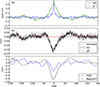 |
Fig. 7. Correlation plots of PSR J1842+0358. Panel a: Auto-correlation curves of the MP and the IP intensities, which reveal the periodicities in the pulse intensities. The plots are zoomed in to the y-range of −0.2 to 0.4. Panel b: Cross-correlation between the MP and the IP single-pulse intensities and its error bars in black line, and the correlation when reversing the order of the single pulses in grey dashed line. The corresponding correlation of the off-pulse regions is in red. Panel c: Correlation plots computed using the running averaged intensities of the MP and the IP, with the FAST sequence in black, and the MeerKAT sequence in blue, respectively. |
To inspect the MP-IP anti-correlation on the single-pulse level, we compute the cross-correlation between the summed intensities of the pulses. The resulted curve is shown in Fig. 7b. The corresponding lags are computed such that a positive lag means the MP lags the IP, and vice versa. The maximum correlation is −0.17 ± 0.01 and appears to occur at a negative lag (but as discussed in Appendix A.3, this lag is insignificant and consistent with zero). The errors on the cross-correlation are determined by random shuffling the pulse order 100 times, determining each shuffled cross-correlation, and taking the standard deviation of those as the error.
Comparing the cross-correlation in panel b and the auto-correlations in panel a in Fig. 7, the long-term variabilities in the MP and especially the IP highly resemble the periodicities in the cross-correlation, although with a different sign at the same lag. This further supports the idea that the long-term variabilities are responsible for the anti-correlation between MP and IP.
To demonstrate the significance of the anti-correlation, we compared it to the cross-correlation of the off-pulse region (in red in panel b). All other aspects of the method were unchanged. The on-pulse anti-correlation is much larger than that of the off-pulse, indicating it is significant and not caused by instrumental effects or RFI. We also checked that the anti-correlation presents in the two halves of the sequence.
From the cross-correlation curve, the most significant feature is that the curve is asymmetric around zero – the first peak with positive correlation appears around 80 lags for positive lags, which is longer than the first positive peak at negative lags around −40 lags. This asymmetry is best seen in Fig. 7b, by comparing against the dashed curve, computed by reversing the order of the pulses. The asymmetry is also visible in the cross-correlation curve of the two halves of the pulse sequence. The behaviour of the correlation curve is further investigated in Sect. 5.1, which is likely to be caused by the different emission patterns in the MP and the IP.
As followed from Fig. 5, the IP intensity difference based on weak and bright MP pulses increases if the running average is used, compared to using the individual pulses. This suggests the long-term variability is responsible for the anti-correlation. To show this, we now also determine cross-correlation using the running averaged method, applied to the FAST and MeerKAT data. In Fig. 7c, the cross-correlation curve of the FAST running-averaged intensities (black) reveals an anti-correlation of increased significance, with a maximum of −0.52 ± 0.01. The curve is similar to that computed with the single-pulse intensities, showing an asymmetry around zero lag, but with a much larger correlation and a more significant quasi-periodicity. The maximum cross-correlation between the MP and the IP running-averaged intensities of the MeerKAT data (blue) is weaker than that of the FAST data. This is because the MeerKAT S/N is lower.
3.7. Summary
Using the FAST data we have shown, from the average profiles constructed from different pulse intensities (Sect. 3.4), and from the cross-correlation analysis (Sect. 3.6), that there is an anti-correlation between the MP and the IP intensities, and that this correlation is caused by the long-term intensity variability. From the spectral analysis (Sect. 3.5), both pulses reveal quasi-periodicity modulation at a long timescale P3 over 100 pulses.
4. PSR J1926+0737
The analysis of PSR J1926+0737 mirrors that of PSR J1842+0358, as detailed in Sect. 3. The subsequent sections present the average profile morphology (Sects. 4.2 and 4.3), the single-pulse analysis using average profiles of different intensities (Sect. 4.4), the fluctuation spectra (Sect. 4.5), and the cross-correlation analysis (Sect. 4.6), respectively.
4.1. TPA pulse stack
The pulse stacks and profiles of PSR J1926+0737 from the MeerKAT TPA data are shown in Fig. 8. The MP shows some modulation, on very long timescales (∼100 P) and not strictly periodic. No clear periodicity is easily identified in the IP emission pattern. From the 2DFS in Song et al. (2023), only the MP has a low-frequency feature, without a clear drift. To determine if the quasi-periodicity in the MP extends to the IP as well, we pursued a higher S/N observation using FAST.
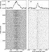 |
Fig. 8. Main pulse (left) and interpulse (right) pulse stacks of PSR J1926+0737. The pulse sequences were averaged over ten single pulses but the pulse number shows the number of single pulses. The corresponding average profiles of all single pulses are shown on the top panels. |
4.2. Average pulse-profile morphology
The MP and IP of this pulsar have asymmetric profiles (top panels in Fig. 9). The 14°-wide MP consists of multiple components. In particular, one component in the trailing part is marked by bright emission in some single pulses. The IP is narrower (≃9°) and consists of a Gaussian convolved with an exponential tail. There is an increase of emission from around pulse longitude 270°, but it is not clear from the single pulses (further discussed in Sect. 4.4) where this originates.
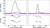 |
Fig. 9. Average pulse profile of PSR J1926+0737 (top) for MP (left) and IP (right). The total intensity profile (normalised by the MP peak) is in black, and the corresponding linear and circular polarisation are shown in red and blue, respectively. The bottom plots show the computed polarisation position angles. |
4.3. Evidence of an orthogonal rotator
The separation between the peak of the MP and the peak of the IP is about 166.3°, smaller than the two-pole expectation of 180°. But the narrowness of the MP and IP profiles and the lack of other, bridging emission, argue for a double-pole pulsar. The divergence from 180° suggests only part of the beam is visible. Figure 9 shows the polarisation profiles and PAs. The PA-swing of the MP forms a V-shape. The IP PAs are mostly flat across the pulse longitude. There is a trend of decreasing PAs towards the trailing part of the pulse profile, but with larger error bars. The PA measured around the pulse profile peak (around 268°) shows a dip that is 100° lower than the other PA points. This point is likely to be insignificant due to the low linear polarisation (in red on the top panel). These are consistent with the findings in Sun et al. (2025).
From these PAs we cannot constrain the sign of β as was done in Sect. 3.3. As the PAs are similar at the MP and IP peaks (∼100°), the pulsar is consistent with an orthogonal rotator however.
4.4. Single-pulse stack
From the pulse stack of the first 1000 pulses in Fig. 10, it is clear that MP (panel a) and IP (panel b) emission show intensity modulation. This modulation lacks a strong pulse longitude variation (i.e. drifting sub-pulses). Whether there are any periodicities within the single pulses or not is not entirely clear from just looking at the pulses (but see Sect. 4.5). The MP seems to have an additional emission around pulse longitude 108°, which coincides with the extra component in the average pulse profile.
4.4.1. Separating bright and weak pulses
The pulse stack (Figs. 10a and 10b) already suggests an MP-IP anti-correlation – around pulse 100, for example, the IP is bright but the MP is nearly undetected, while near pulse 150 it is the opposite. As in Sect. 3.4.1 we separate weak and bright pulses, now at the 50th percentile of pulse energy. Blocks of strong emission are seen in Figs. 10a–c for the MP around pulse 100, 210, and for the IP around pulse 0 to 50, around 200. The single-pulse intensities also show some spiky structures.
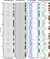 |
Fig. 10. First 1000 single pulses for PSR J1926+0737. Pulse stacks (MP, IP) and intensities (single-pulse, running average). Panel a: Pulse stack of the MP. The blue and green margin bars mark the bright pulses, based on the intensities of the single pulses (blue, left) or their running averages (green, right). Panel b: Same as (a) but for the IP, now with violet and brown for single-pulse and running-averaged intensities, respectively. Panel c: Single-pulse intensities of the MP and the IP, with the running averaged intensities plotted on top. Margin bars identical to the left of (a) and (b). Panel d: Running averaged intensities of the MP and the IP plotted alone, along with the corresponding selected bars (the same as those on the right of a and b). The rest of the PSR J1926+0737 pulse stacks are available online. |
The single-pulse energies (Fig. 11) again show no significant bi-modality (and thus, no evidence of a mode change). For 11 single-pulse running-averaged intensities, the distributions are narrower. With these running-averaged intensities (Fig. 10d), the long-term variations become much more significant. The selected 50-percentile bright and weak blocks of the MP and the IP are now clearly anti-correlated.
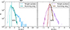 |
Fig. 11. Pulse energy distributions of PSR J1926+0737 for MP (left) and IP (right), with single-pulse energies (blue and violet) and running-averaged pulse energies (green and brown). Both pulse energies are normalised by the mean MP energy. The vertical line shows two groups that are split at the median pulse intensity (as described in Sect. 4.4.1). |
4.4.2. (Anti-)correlation between the MP and IP brightness
This MP and IP anti-correlation is further demonstrated when again averaging profiles when the opposite pulse is weak or bright (Figs. 12a and 12b). The MP is brighter when the IP is in its weaker half from the running average (dark red). It is weaker when the IP is bright (brown) – corroborating the MP-IP intensity anti-correlation. The difference in running-averaged-based intensities is larger than in the single-pulse-constructed profiles (see the full version in Figs. A.2c and A.2d). This indicates that the long-term variability in the IP correlates strongly to the MP intensity variation, rather than the stochastic variability. The IP average profiles in panel b lead to exactly the same conclusions. The shape of the profile does not significantly change (see a further description in Fig. A.2). Our first and last-half sequence tests, finally, confirm our finding: the anti-correlation is real and always present. Longitude-resolved cross-correlation maps again corroborate the result (Appendix A.2).
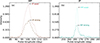 |
Fig. 12. Average profiles of MP and IP of PSR J1926+0737 based on grouping pulses by the brightest and weakest halves of the opposite pulse. Panel a: MP profiles based on, from top to bottom: weakest IP in running averaged (dark red), then brightest IP in running averaged (brown) marked in Fig. 11b. Panel b: IP average pulse profiles, based on the MP halves, with colours in cyan and green, as marked in Fig. 11a. An anti-correlation is clearly present. |
In this section we have shown, through constructing the average profiles of the bright and weak groups of the pulses, that the brightness of the MP and IP are anti-correlated. This anti-correlation is present along all on-pulse longitudes and is maintained over a long time. Moreover, it is the long-term variability in the MP and the IP that is responsible for the anti-correlation. The quasi-periodicity will be investigated next.
4.5. Probing the quasi-periodic modulations
The intensity variations in Fig. 10d suggest (quasi-)periodic single-pulse modulation. As described in Sect. 3.5 these can be revealed using the LRFS and 2DFS (Fig. 13).
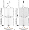 |
Fig. 13. Fluctuation spectra of PSR J1926+0737 for MP (left) and IP (right). For a full description, see Fig. 6. |
The top panel shows the MP (left column) modulation is mostly flat in the leading part, with indices ∼1.7, followed by an increase. As the IP is weaker, the modulation is less constrained, but still trends up. Indices are relatively high (≳1), indicating clear single-pulse intensity variability. The FAST data, with clearly detected and variable single pulses, produce larger MP modulation indices, with smaller errors, than the MeerKAT data.
The main LRFS (middle panels) features are below 0.02 cpp and result in a periodicity ≃153 ± 55 from the MP, and ≃147 ± 63 for the IP. The single-pulse stack (Fig. 10) also suggests shorter-term, tens-of-pulses intensity variability, but there is no clear feature in the LRFS. Stochastic variabilities towards higher 1/P3 frequencies (e.g. from 0.02 to 0.3 cpp) are seen as a red-noise spectrum, due to the intensity changes in the single pulses. Possibly, this short-term variability has an unstable timescale and is washed out by the longer-term (a few hundred P) modulation.
The 2DFS (bottom panels of Fig. 13) indicates some overall negative drift for MP and IP, but it is not clearly associated with the lowest modulation frequency. Therefore, the dominant variability is longitude stationary. This is corroborated by the sub-pulse phase tracks (Appendix A.4).
4.6. Timescales of the correlated emission
Correlations between the MP and IP summed intensities can determine the timescales and delays of the quasi-periodicities. Figure 14a indicates a peak-to-peak periodicity of about 120P, consistent with the higher frequency spectral feature in the LRFS and the 2DFS. In the MP, the second minimum appears around lag 150, with further positive peaks around lag 240. This indicates that the periodicities are unstable.
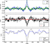 |
Fig. 14. Correlation plots of PSR J1926+0737. Panel a: Auto-correlation curves of the MP and the IP intensities, which reveal any periodicities in the pulse intensities. The plots are zoomed-in to the y-range of −0.1 to 0.2. Panel b: Cross-correlation between the MP and the IP single-pulse intensities and its error bars in black line, and the correlation when reversing the order of the single pulses in grey dashed line. The corresponding correlation of the off-pulse regions is in red. Panel c: Correlation plots computed using the running averaged intensities of the MP and the IP, with the Fast full sequence in black, and the MeerKAT full sequence in blue, respectively. |
To next investigate if there exist time delays in the MP-IP interaction, we determine their intensity cross-correlation at different lags (Fig. 14b, black line). The maximum anti-correlation is −0.13 ± 0.02, which is significantly larger than the reference off-pulse correlation (red) at a positive lag (but it is consistent with zero lag; see Appendix A.3). This anti-correlation is also present in the two halves of the sequence (not shown).
The cross-correlation based on the reversed pulse order reveals no significant asymmetry (Fig. 14b). This differs from PSR J1842+0358 (Fig. 7), where the modulation in the IP featured a fast rise and slow fade. In addition, the periodicity in the cross-correlation is very similar to those in the auto-correlations of the MP and the IP, confirming the single-pulse quasi-periodicity.
Applying these same methods on the running averages instead of the single pulses results in an even larger maximum correlation of −0.50 ± 0.02 (Fig. 14c, black for FAST observation). The MeerKAT observation also reveals an anti-correlation around zero lag, with the cross-correlation curve in blue. This validates that the long-term variability (not the short-term changes) is the reason for the MP-IP anti-correlation.
4.7. Summary
We established that PSR J1926+0737 shows an anti-correlation between the MP and the IP, both of which display quasi-periodic changes on timescales of > 100 pulses. The quasi-periodicities do not display sub-pulse phase modulations, in contrast to the sub-pulse drift in the IP of PSR J1842+0358.
5. Discussion
In the following, we discuss the established emission correlations. Possible interpretations are then considered.
5.1. Simulating the cross-correlation curve of J1842+0358
The cross-correlation curves of PSR J1842+0358 (Figs. 7b, c) show a number of interesting features. The large anti-correlation near lag 0 is asymmetric, so that the negative correlation extends farthest to positive lags. A positive correlation appears on either side of this central negative correlation, but the peak on the right-hand side is located about twice as far from lag 0 as that on the left. Here we show that these asymmetries can be explained by the MP and IP having different intensity modulation patterns in their variability cycles.
To demonstrate this, we simulated a sequence of MP and IP intensities to mimic their behaviour within one P3 period. Instead of assuming any analytic description of these sequences, we used the measurements directly. A complication is that the modulation cycle is variable. To deal with this, the pulse stacks for the MP and IP were classified by eye in bright and weak sequences. Because each sequence had a different length, interpolation was used to combine the individual sequences. The result is a single averaged bright and weak mode sequence for the MP and IP, with a length equal to their median length.
We established that the MP and IP share an identical P3 periodicity (Sect. 3.5). Therefore, to explain the correlations, the brightening and weakening of the MP and IP during the P3 cycle must follow a typical and repeated structure. Here we simulate this repeated periodic structure, without cycle-to-cycle variability. The length of the MP and IP cycle are scaled to be the same to reflect the synchronisation of the P3 periodicities. To reproduce the anti-correlation, the MP starts in the weak sequence, while the IP starts in the bright sequence.
Two cycles of the obtained sequence are shown in the left panel of Fig. 15. This reveals that the MP (blue) shows a relatively sharp and symmetric brightening profile during the modulation cycle. On the other hand, the IP (green) shows a sharp rise in intensity followed by a gradual fall. This behaviour is also visible in the average intensities shown in panel d of Fig. 3. For example, around pulse 200, 300, 550 and 750, the MP average intensities are bright and the bright IP intensities follow. The simulated sequences agree well with the (2/3, 1/3) weak and bright duration split adopted in Sect. 3.4.1.
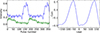 |
Fig. 15. Left: Simulated pulse-intensity sequence within two P3 cycles of MP (blue) and IP (green) obtained as the average of selected single pulses (see text for details). Right: Corresponding cross-correlation curve. |
The cross-correlation curve obtained from the simulated sequences is shown in the right panel of Fig. 15. Important observed features are reproduced: the negative correlation around zero lag is asymmetric. A positive correlation also appears at a negative lag of −49 pulses, and at a positive lag of 134 pulses, that is, nearly twice as large. This is because in the simulated intensity sequence the bright MP phase occurs just before the sharp rise in the IP intensity and well after the preceding bright IP phase. This simulation confirms that the observed MP-IP intensity correlations arise from slow, phase-locked P3 modulation.
5.2. Longitude stationary modulation
The two pulsars discussed in this paper reveal that the main and inter-pulse emission possess the same sub-pulse modulation periodicity. In addition, at least the modulation in one pulse is longitude stationary. Longitude stationary modulation is observed in other inter-pulse pulsars that show main and inter-pulse communication. In particular for those with evidence of orthogonal rotators, PSRs B1702−19 (Weltevrede et al. 2007), B1055−52 (Weltevrede et al. 2012), and B1822−09 quiet mode (Yan et al. 2019) have longitude stationary features for their MP and IP emission. PSR B0823+26 (Chen et al. 2023) shows drifting sub-pulses in the MP while the IP is longitude stationary. All six orthogonal rotators with main-inter-pulse communication (including the two pulsars studied here) have longitude stationary modulation. This suggests that having longitude stationary modulation in at least one of the two pulses is common, if not universal, for orthogonal rotators exhibiting sub-pulse modulation.
The presence of longitude stationary modulation in these inter-pulse pulsars can be contrasted with longitude stationary modulation found in the general pulsar population. Therefore, all pulsars with Ė ≥ 1032 erg/s – above which the six inter-pulse pulsars with orthogonal geometry and periodic sub-pulse modulation are found – were selected. Of those pulsars for which also periodic sub-pulse modulation was detected, about 40% had at least one profile component with longitude stationary modulation (estimated from Song et al. 2023). Thus the probability of finding longitude stationary features in six out of six inter-pulse pulsars with periodic modulation by chance is small. This suggests that sub-pulse modulation in orthogonal rotators could well be different compared to the general population of pulsars.
The nearly orthogonal geometry might well be important because this geometry leads to a different current distribution and variation in the accelerating potential across the polar cap (see e.g. Fig. 1 in Timokhin & Arons 2013) compared to aligned rotators. Because the spark drift is governed by this potential variation (Szary & van Leeuwen 2024), the resulting sub-pulse motion in orthogonal rotators might be affected, leading to longitude stationary modulation only.
5.3. Model interpretation
We established that the sub-pulse modulations in the MP and IP of PSRs J1842+0358 and J1926+0737 are synchronised. The MP and IP share the same P3, and despite P3 not being strictly constant, the modulation patterns of the MP and IP remain phase-locked. Therefore, the two pulsars studied here add to a fundamental problem with the text-book picture of pulsar emission. The MP and IP are normally assumed to come from open field lines anchored to opposite magnetic poles, and it is the local polar cap physics that is thought to be responsible for sub-pulse modulation. To maintain phase locking, the emission regions responsible for the MP and IP emission need to have some means of inter-communication.
In searching for a model, the simplest assumption would be to assign identical and completely synchronised emission regions to MP and IP and attribute the observed apparent asymmetry to differing LoS cuts through the emission beams. The widespread observations of a complex and often subtle asymmetry in these pulsars (including the longitude stationary modulation features discussed in Sect. 5.2) seems to call this into question, however.
An alternative view is to see the MP and IP together forming a single inter-connected system but with the MP and IP playing different roles so that the modulation arising from each driving, with delay, modulation in the other, thus creating, in effect, a hysteresis loop. Evidence of this behaviour is suggested in PSR J1842+0358 by brief but intense emission at the MP triggering a sudden enhancement of intensity and sub-pulse drift at the IP. In turn, the bright stationary emission is restarted in the MP as the drift process fades. This would result in the quasi-periodic periodicity at both poles demonstrated by the simulation in Fig. 15.
In the following, we explore a range of potential mechanisms in light of these possibilities. The models considered include: firstly, emission from the main and inter-pulse are from the opposite poles, with the interaction through the large-scale magnetosphere. Secondly, there is an external driver responsible for the periodicities at both poles. Lastly, a single-pole mechanism may be able to avoid the need for inter-pole communication.
5.3.1. Inter-pole communication
Over the years pulsar magnetosphere models have been theoretically examined and modelled. Generally it has been assumed that the magnetosphere is in a steady state with the implicit assumption that the observed complex radio emission patterns are a small-scale perturbation (e.g. sparks) to the model.
In this picture the magnetosphere has two distinct zones: open field lines extending to infinity and a closed region connecting the magnetic poles with zero potential difference and a trapped corotating plasma. In cases where the pulsar is near-aligned, Ruderman & Sutherland (1975) postulated that there is a plasma E × B drift across the open field lines so that it lags corotation with a periodicity P4 ∼ 5.6B/P2 (where B is the dipolar magnetic field in units of 1012 G). It is reasonable to expect a periodicity of this order even when the pulsar is highly inclined, although, as we point out above, the simple picture of the RS model has to be significantly adapted for these pulsars.
The lag increases as the pulsar ages until, in old pulsars, its theoretical value becomes comparable to the spin of the star. But for middle-aged pulsars such as J1842+0358 and J1926+0737, the expected lag is quite modest, being 45P and 19P respectively. These figures are significantly smaller than the modulation timescales observed here, but can be lengthened within the RS framework by adopting a smaller closed region and hence a polar cap radius wider by a factor s giving P4 ∼ 5.6s2B/P2. This would suggest s ∼ 2 or 3. A extended emission region like this has been inferred observationally for PSR B1055−52 (Weltevrede & Wright 2009), where polarimetry suggests that the MP emission originated from regions between s = 1.5 and s = 2.
The challenge presented by these pulsars is therefore not so much the timescale of the modulations but the fact that they demonstrate strong communication between the poles, which are traditionally thought to be separated by field lines enclosing an inactive corotating plasma. We are therefore compelled to abandon the assumption that the magnetospheres of these pulsars are in a steady state, even on the inter-pole travel timescale of one pulse period (Biggs 1990). The important further implication is that if inter-pulse pulsars have proven interaction between their poles, then we may suppose that other (maybe all) pulsars have interactive magnetospheres (as argued by Melrose & Yuen 2012, 2016; Wright 2022 and by Basu et al. 2020 from observational evidence). In this picture, the observed emission patterns are created by the interactions themselves.
In highly inclined pulsars, the MP and IP beam will have a central region (not necessarily defined by the last closed field line touching the light cylinder) whose field lines drive the angular momentum loss of the pulsar to infinity. But the field lines which generate the outer regions of the beam (i.e. those that communicate between poles via closed field lines) will have a strongly differing physical environment, depending on whether they are equatorial with respect to the rotation axis and pass close to the light cylinder, or perpendicular to the equator and pass close to the rotation axis itself (well within the light cylinder). Even the equatorial regions themselves will likely be asymmetric since the trailing and leading field lines will carry particle flow with or counter to the pulsar rotation.
Thus any polar beam will have at least three or four distinct regions with separate emission characteristics, and the separate LoS at MP and IP will probably sample very different regions, even if the beams are intrinsically identical at each pole. This is potentially a way to explain why longitude stationary modulation is observed at one pole and drift with the same modulation at the other. Different geometries give rise to distinct signatures in the polarisation profiles, reflecting how the LoS intersects the emission beams. As already discussed in Hankins & Cordes (1981), for a strictly orthogonal rotator, the MP and IP arise from the same hemisphere (same side of the beam), and their PA swings should have slopes of the same sign. On the other hand, for a nearly orthogonal rotator, the LoS can trace opposite sides of the MP and IP beam, yielding opposite slopes of the PA swings. In PSR J1842+0358 (Sect. 3.2), the opposite PA-swing slopes indicate that we are probably viewing field lines on opposite sides of the beam axis. PSR J1926+0737 is less conclusive given its complicated changes in the PAs across the pulse profile (Sect. 4.2). The handedness of circular polarisation can provide an additional indication of the emission hemisphere (e.g. Johnston & Kramer 2019). For the two pulsars discussed here, however, the circular polarisation of the IP is too weak to draw any meaningful conclusions.
The physics behind inter-pole interaction, although argued to be widespread on geometric and observational grounds (Wright 2022), has been little studied. Global changes in the magnetosphere have been suggested to explain correlated changes in the pulsar spin-down rate and the pulse shape (e.g. Kramer et al. 2006; Lyne et al. 2010). And it should be pointed out that the simultaneous radio and X-ray mode change in PSR B0823+26 (Hermsen et al. 2018), a pulsar now known to have simultaneous modulations at both poles in radio on timescales of a few pulse periods (Chen et al. 2023), is a clear indication of a magnetosphere which undergoes dramatic but not understood physical changes. An potential route to connect the two magnetic poles would be via the return current (e.g. Beskin et al. 2017).
5.3.2. Extrinsic drivers
The fact that MP and IP emission show the same periodicity could point towards an external mechanism driving the modulation in both emission regions. This mechanism could be material external to the pulsar interacting with the magnetosphere. This material might come from regions connected to the neutron star magnetosphere. For example, Philippov et al. (2015, 2019) and Lyubarsky (2019) considered magnetic reconnection around a Y-shaped current sheet just outside the light cylinder, and this may provide a viable way of influencing both poles via a return current.
Other external materials could be provided by a fallback disk formed when the star was born (Michel & Dessler 1981). As discussed by Cordes & Shannon (2008), this fallback disk, circulating around the neutron star, might be in the form of asteroids (rocks). These materials need to be within the light cylinder to influence the emission. Given the modulation periodicity around 100 pulses for PSRs J1842+0358 and J1926+0737, the corotation radii of the two pulsars are outside the light cylinder. Interaction can only be expected if asteroids come within the light cylinder, a scenario that could be possible, despite the long periodicities, if the asteroids are in a highly elliptical orbit. The existence of asteroids has been suggested to explain the emission changes in PSR J0738−4042 (Brook et al. 2014).
If indeed the synchronised modulation in the MP and IP are caused by a single external driving mechanism, some asymmetry between the poles will be required unless caused by difference in the way the LoS crosses the emission beams. Otherwise, asymmetries could arise from the orientation of the inflow of material (e.g. the orientation of the orbit of an asteroid or the return current). An extrinsic model gives a natural explanation of the synchronisation, as the external materials interact with the magnetosphere similarly for different emission regions.
5.3.3. Single-pole mechanism
In the standard picture, the MP and IP emission are produced at opposite poles, making inter-pole communication difficult to explain. As suggested by Dyks et al. (2005a), however, this issue can be avoided if the MP and IP emission come from the same pole. Then one pulse is composed of outward, and the other of inward directed emission. The inward emission travels through the magnetosphere, past the neutron star, and is seen half a turn later4. This model was proposed to explain the anti-correlation between the IP and the pre-cursor of PSR B1822−09.
In a single-pole interpretation the MP and IP are not expected to be exactly 180° apart, the inward emission has to travel further as it needs to pass the neutron star before reaching the observer. This could explain why for the two pulsars discussed in this paper the MP-IP separation deviates from 180°. The inward emission is expected to be delayed relative to the outward emission (Dyks et al. 2004, 2005a,b). This leads us to conclude that for both our pulsars, since the separation between the MP and the IP is less than 180°, the MP is dominated by inward directed emission, and the IP by outward directed emission. The required emission heights (Dyks et al. 2004, 2005a; Weltevrede et al. 2007) are of the order of a few hundred kilometres. These emission heights are compatible with those estimated from polarisation properties of many pulsars (e.g. Rookyard et al. 2015).
Most importantly, the single-pole model avoids the need for communication between emission regions far apart. The two pulses possess synchronised modulation would be naturally explained because the two pulses originate from the same region in the magnetosphere. The model lacks a physical motivation for why the inward emission should be produced, however, and how emission can propagate through the inner magnetosphere with strong magnetic fields (Dyks et al. 2005a). In addition, it is not clear why inward emission is only seen in one pole but not the other.
6. Conclusions
The high sensitivity of FAST allowed us detailed observations of two new inter-pulse pulsars. Strikingly, each of these two pulsars shows a similar behaviour: The quasi-periodicity is the same for the MP and the IP, and their modulation is anti-correlated. The periodicity is long, about 100 pulses. The (anti-)correlation is clearly visible in the average pulse profiles of the bright and dim pulse groups, whose intensity is brighter when the weak pulses of the opposite pole were selected. The further correlation analysis confirmed the result, and the correlation was maintained over a time span of several years.
One interesting but poorly understood phenomenon in all inter-pulse pulsars with interaction is that the modulation of one pulse is stationary in longitude. This might be a requirement for communication between two emission regions. It further requires that the model can provide some form of asymmetry to allow different behaviours from the two emission regions.
Important evidence of the underlying emission mechanism is provided by studying inter-pulse pulsars. the MP-IP interaction is not predicted by a simple rotating carousel model, which is local and confined within the polar cap regions. The interaction requires some global changes, which might be fulfilled by an interactive magnetosphere. We conclude that an interactive magnetosphere is common to all pulsars, and that MP-IP communication and the correlation between the spin-down rate and the long-term pulse shape variations are observational manifestations.
Data availability
Appendices B and C that provide the full pulse stacks of PSRs J1842+0358 and J1926+0737 are available at 10.5281/zenodo.17816012.
Acknowledgments
We thank L. Wang and F. Kou for their support at the FAST proposal stage, and for assistance with the data transfer. We further thank the investigators of PT2023_0052 for their useful data. This research was supported by Vici project ‘ARGO’ with project number 639.043.815 and by ‘CORTEX’ (NWA.1160.18.316), under the research programme NWA-ORC; both financed by the Dutch Research Council (NWO). This work made use of the data from FAST (Five-hundred-meter Aperture Spherical radio Telescope) (https://cstr.cn/31116.02.FAST). FAST is a Chinese national mega-science facility, operated by National Astronomical Observatories, Chinese Academy of Sciences. The MeerKAT telescope is operated by the South African Radio Astronomy Observatory, which is a facility of the National Research Foundation, an agency of the Department of Science and Innovation.
References
- Backer, D. C. 1970, Nature, 227, 692 [Google Scholar]
- Backus, I., Mitra, D., & Rankin, J. M. 2010, MNRAS, 404, 30 [NASA ADS] [Google Scholar]
- Basu, R., Mitra, D., Melikidze, G. I., et al. 2016, ApJ, 833, 29 [Google Scholar]
- Basu, R., Mitra, D., Melikidze, G. I., & Skrzypczak, A. 2019, MNRAS, 482, 3757 [NASA ADS] [CrossRef] [Google Scholar]
- Basu, R., Mitra, D., & Melikidze, G. I. 2020, ApJ, 889, 133 [Google Scholar]
- Beskin, V. S., Galishnikova, A. K., Novoselov, E. M., Philippov, A. A., & Rashkovetskyi, M. M. 2017, J. Phys. Conf. Ser., 932, 012012 [Google Scholar]
- Biggs, J. D. 1990, MNRAS, 246, 341 [NASA ADS] [Google Scholar]
- Biggs, J. D., Lyne, A. G., Hamilton, P. A., McCulloch, P. M., & Manchester, R. N. 1988, MNRAS, 235, 255 [Google Scholar]
- Brook, P. R., Karastergiou, A., Buchner, S., et al. 2014, ApJ, 780, L31 [Google Scholar]
- Chen, J. L., Wen, Z. G., Duan, X. F., et al. 2023, ApJ, 946, 2 [Google Scholar]
- Chernoglazov, A., Philippov, A., & Timokhin, A. 2024, ApJ, 974, L32 [Google Scholar]
- Cordes, J. M., & Shannon, R. M. 2008, ApJ, 682, 1152 [NASA ADS] [CrossRef] [Google Scholar]
- Desvignes, G., Kramer, M., Lee, K., et al. 2019, Science, 365, 1013 [Google Scholar]
- Dyks, J., Rudak, B., & Harding, A. K. 2004, ApJ, 607, 939 [NASA ADS] [CrossRef] [Google Scholar]
- Dyks, J., Zhang, B., & Gil, J. 2005a, ApJ, 626, L45 [NASA ADS] [CrossRef] [Google Scholar]
- Dyks, J., Frąckowiak, M., Słowikowska, A., Rudak, B., & Zhang, B. 2005b, ApJ, 633, 1101 [Google Scholar]
- Eatough, R. P., Molkenthin, N., Kramer, M., et al. 2010, MNRAS, 407, 2443 [NASA ADS] [CrossRef] [Google Scholar]
- Edwards, R. T., & Stappers, B. W. 2002, A&A, 393, 733 [NASA ADS] [CrossRef] [EDP Sciences] [Google Scholar]
- Fowler, L. A., & Wright, G. A. E. 1982, A&A, 109, 279 [NASA ADS] [Google Scholar]
- Gil, J. A., Jessner, A., Kijak, J., et al. 1994, A&A, 282, 45 [NASA ADS] [Google Scholar]
- Hankins, T. H., & Cordes, J. M. 1981, ApJ, 249, 241 [NASA ADS] [CrossRef] [Google Scholar]
- Hermsen, W., Kuiper, L., Basu, R., et al. 2018, MNRAS, 480, 3655 [NASA ADS] [CrossRef] [Google Scholar]
- Jiang, P., Yue, Y., Gan, H., et al. 2019, Sci. China Phys. Mech. Astron., 62, 959502 [NASA ADS] [CrossRef] [Google Scholar]
- Johnston, S., & Kramer, M. 2019, MNRAS, 490, 4565 [NASA ADS] [CrossRef] [Google Scholar]
- Johnston, S., Karastergiou, A., Keith, M. J., et al. 2020, MNRAS, 493, 3608 [NASA ADS] [CrossRef] [Google Scholar]
- Kou, F. F., Yan, W. M., Peng, B., et al. 2021, ApJ, 909, 170 [Google Scholar]
- Kramer, M., & Johnston, S. 2008, MNRAS, 390, 87 [NASA ADS] [CrossRef] [Google Scholar]
- Kramer, M., Lyne, A. G., O’Brien, J. T., Jordan, C. A., & Lorimer, D. R. 2006, Science, 312, 549 [NASA ADS] [CrossRef] [Google Scholar]
- Lorimer, D. R., Faulkner, A. J., Lyne, A. G., et al. 2006, MNRAS, 372, 777 [NASA ADS] [CrossRef] [Google Scholar]
- Lyne, A., Hobbs, G., Kramer, M., Stairs, I., & Stappers, B. 2010, Science, 329, 408 [NASA ADS] [CrossRef] [Google Scholar]
- Lyubarsky, Y. 2019, MNRAS, 483, 1731 [NASA ADS] [CrossRef] [Google Scholar]
- Maciesiak, K., Gil, J., & Ribeiro, V. A. R. M. 2011, MNRAS, 414, 1314 [NASA ADS] [CrossRef] [Google Scholar]
- Melrose, D. B., & Yuen, R. 2012, ApJ, 745, 169 [NASA ADS] [CrossRef] [Google Scholar]
- Melrose, D. B., & Yuen, R. 2016, J. Plasma Phys., 82, 635820202 [CrossRef] [Google Scholar]
- Michel, F. C., & Dessler, A. J. 1981, ApJ, 251, 654 [Google Scholar]
- Nan, R., Li, D., Jin, C., et al. 2011, Int. J. Mod. Phys. D, 20, 989 [Google Scholar]
- Philippov, A. A., Spitkovsky, A., & Cerutti, B. 2015, ApJ, 801, L19 [NASA ADS] [CrossRef] [Google Scholar]
- Philippov, A., Uzdensky, D. A., Spitkovsky, A., & Cerutti, B. 2019, ApJ, 876, L6 [NASA ADS] [CrossRef] [Google Scholar]
- Radhakrishnan, V., & Cooke, D. J. 1969, Astrophys. Lett., 3, 225 [NASA ADS] [Google Scholar]
- Rankin, J. M. 1986, ApJ, 301, 901 [Google Scholar]
- Rankin, J. M., & Rathnasree, N. 1997, JApA, 18, 91 [NASA ADS] [Google Scholar]
- Rookyard, S. C., Weltevrede, P., & Johnston, S. 2015, MNRAS, 446, 3367 [NASA ADS] [CrossRef] [Google Scholar]
- Ruderman, M. A., & Sutherland, P. G. 1975, ApJ, 196, 51 [Google Scholar]
- Song, X., Weltevrede, P., Szary, A., et al. 2023, MNRAS, 520, 4562 [NASA ADS] [CrossRef] [Google Scholar]
- Sun, S. N., Wang, N., Yan, W. M., & Wang, S. Q. 2025, ApJ, 983, 179 [Google Scholar]
- Szary, A., & van Leeuwen, J. 2024, MNRAS, 532, 4075 [Google Scholar]
- Timokhin, A. N., & Arons, J. 2013, MNRAS, 429, 20 [NASA ADS] [CrossRef] [Google Scholar]
- van Leeuwen, J., & Timokhin, A. N. 2012, ApJ, 752, 155 [NASA ADS] [CrossRef] [Google Scholar]
- van Leeuwen, J., Kasian, L., Stairs, I. H., et al. 2015, ApJ, 798, 118 [NASA ADS] [CrossRef] [Google Scholar]
- Wang, H., Keith, M. J., Weltevrede, P., et al. 2025, MNRAS, 544, 234 [Google Scholar]
- Weltevrede, P. 2016, A&A, 590, A109 [NASA ADS] [CrossRef] [EDP Sciences] [Google Scholar]
- Weltevrede, P., & Wright, G. 2009, MNRAS, 395, 2117 [NASA ADS] [CrossRef] [Google Scholar]
- Weltevrede, P., Edwards, R. T., & Stappers, B. W. 2006, A&A, 445, 243 [NASA ADS] [CrossRef] [EDP Sciences] [Google Scholar]
- Weltevrede, P., Wright, G. A. E., & Stappers, B. W. 2007, A&A, 467, 1163 [NASA ADS] [CrossRef] [EDP Sciences] [Google Scholar]
- Weltevrede, P., Wright, G., & Johnston, S. 2012, MNRAS, 424, 843 [Google Scholar]
- Wright, G. 2022, MNRAS, 514, 4046 [Google Scholar]
- Yan, W. M., Manchester, R. N., Wang, N., et al. 2019, MNRAS, 485, 3241 [NASA ADS] [CrossRef] [Google Scholar]
The long-term variability mentioned here and elsewhere refers to single pulses, typically on the order of 100 pulses. This should be distinguished from long-term mode changes in pulse profile shapes that occur over weeks to years.
Since the magnetic field projection on the sky is the same for inward and outward directed emission, the RVM prediction for the PA swing of both are identical (Dyks et al. 2005b).
Appendix A: Additional analysis details
A.1. Anti-correlation between the MP and IP brightness
As discussed in Sects. 3.4.2 and 4.4.2, anti-correlation is revealed by constructing the average pulse profiles based on the strong and weak running averaged intensity of the other pulse. For completeness, we describe the set of average profiles based on the single-pulse intensity groups, and those of normalised profiles to see any possible shape changes.
Figures A.1a and A.1b show the MP and IP normalised pulse profiles using either the single-pulse or running-averaged intensities, respectively. The colours corresponds to those in Fig. 4 for the weak and bright groups. The mean pulse profile is also shown for comparison. The MP average profiles based on bright pulses are wider than those based on weak pulses (in green and blue for single-pulse intensities and running-averaged intensities, respectively). Bright MP pulses having larger pulse widths is a signature of the single pulses as well (as in Fig. 3). In the IP (panel b), the trailing component of the brighter pulses is wider than that of the weaker pulses. This suggests that the bright pulses tend to be brighter at the trailing part of the IP profile. In contrast, the IP profiles constructed with the MP intensities do not show this difference in the trailing component. We speculate that because of the drifting sub-pulses in the IP (see the analysis in Sect. 3.5), bright pulses are more likely to start from the trailing part of the pulse profile (transitioning from weak to bright pulses). While when using the MP weak pulses, the corresponding IP pulses selected include all pulse phases, without a preference of the pulses with a bright trailing component.
Panel c and d give the same set of plots as in Fig. 5 but now include the profiles constructed by the single-pulse intensities. These profiles are constructed using the other pulse, and therefore, the colours we used correspond to the other pulse. The MP intensity difference between profiles constructed based on the running averaged intensities of the IP is larger than those based on the single-pulse intensities (and is also true for the IP). This leads us to conclude that the long-term variability is responsible for the anti-correlation between the MP and the IP.
These sets of profiles are also normalised to see any shape changes (in panels e and f). Visible there is that when the IP is weak, the MP profiles are wider, in both the leading and trailing part (panel e). The IP profile shape does not significantly change with MP weak versus bright.
The same sets of plots but for PSR J1926+0737 are shown in Fig. A.2. The MP and IP peak-normalised average profiles using the bright and weak intensities are in panels a and b, respectively. There is no significant change in the profile shape.
Panels c and d show the average profiles of the weak and bright intensities of the other pulse, the same as in Fig. 12 but adding the profiles based on the single-pulse intensities. Again, the intensity difference is larger between the profiles based on the weak and bright running averaged intensities, comparing to those based on the single-pulse intensities, for both the MP and the IP. This suggests that the long-term variability is strongly correlated, rather than the stochastic variability.
Lastly as in panels e and f, the normalised version of profiles are shown. These do not reveal significant shape changes, which could be because the longitude stationary modulation does not have significant phase variation.
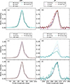 |
Fig. A.1. Average pulse profiles of MP and IP of PSR J1842+0358 based on groups of pulses with different intensities. Panel a: MP peak-normalised average profiles of the bright and weak single-pulse intensities (blue and light blue) and running-averaged intensities (green and cyan), respectively. The average profile in black is also shown. Panel b: Same as (a) but IP peak-normalised average profiles, single-pulse intensities in violet and pink, and running averaged intensities in brown and dark red, respectively. Panel c: MP averaged profiles based on the weakest (dotted) and brightest (dashed) groups of single-pulse intensities and the running averaged intensities of the IP. Colours corresponds to the IP colours in (b). Panel d: Same as (c) but for the IP averaged profiles based on the two groups of the MP. Panels e and f: Same as (c) and (d) but now peak-normalised. |
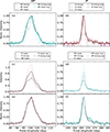 |
Fig. A.2. Average pulse profiles of MP (first column) and IP (second column) of PSR J1926+0737 based on groups of pulses with different intensities. See the caption of Fig. A.1 for details of each panel. |
A.2. Longitude-resolved correlation maps
We can further visualise the anti-correlation found in Sects. 3.4.2 and 4.4.2 by computing the longitude-resolved cross-correlation between the MP and the IP, at zero (or non-zero) phase delay. This is done by calculating the cross-correlation between each pair of intensities in the pulse profile for the single-pulse sequence. At zero delay, strong positive correlation is expected between the on-pulse of the MP and the IP themselves (as auto-correlations). On the other hand, negative correlations are seen between the MP and the IP, clearly confirming the MP and the IP anti-correlation. The longitude-resolved correlation maps for the FAST observation and the MeerKAT observation are presented in Figs. A.3 and A.4 for PSR J1842+0358, and Figs. A.5 and A.6 for PSR J1926+0737, respectively. These are at lag zero. All display an anti-correlation between MPs and IPs. The results from both sets of observations, taken years apart, prove that the anti-correlation is maintained over timescales of years. The behaviour is intrinsic to the pulsar and is not caused by instrumental effects.
The longitude-resolved correlation plots for the FAST data and the ten single-pulse-averaged MeerKAT data are in In these plots, the bottom-left and top-right corners show the auto-correlations between the on-pulse of the MP and the IP, respectively. Strong positive correlations (in red) are present there for all observations. Negative correlations are seen in the top-left corner (in blue), representing the relation between the IP and the MP (mirrored bottom-right, correlation between the MP and the IP). This clearly confirms that the MP and IP are anti-correlated for both pulsars.
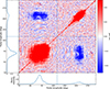 |
Fig. A.3. Longitude-resolved correlation map of PSR J1842+0358 at zero phase delay, and only the selected on-pulse regions are shown (note that the pulse longitudes are not consecutive, where the off-pulse regions are removed). The colour plot shows the corresponding cross correlations along pairs of pulse longitude. The side and bottom panels are the normalised integrated pulse profiles, with the dashed lines indicate boundary of the MP and the IP. |
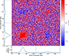 |
Fig. A.4. Longitude-resolved correlation map of PSR J1842+0358 at zero phase delay using the MeerKAT ten-pulse averaged data. Layout otherwise as Fig. A.3. |
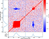 |
Fig. A.5. Longitude-resolved correlation map of PSR J1926+0737 at zero phase delay. Layout otherwise as Fig. A.3. |
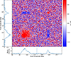 |
Fig. A.6. Longitude-resolved correlation map of PSR J1926+0737 at zero lag using the MeerKAT ten-pulse averaged data. See the caption of Fig. A.2 for further details. |
A.3. Lag of maximum correlation
For both pulsars, we found that the lags where the maximum anti-correlation occurs are not at zero, but we argue here that they are likely consistent with zero. This is because, firstly, the lags at the correlation maximum are different for the two halves of the data. Secondly, we fit the correlation with a parabolic curve at small lags (between −10 to 10 lags) and find that the peak is consistent with zero. For PSR J1926+0737, the parabolic fit to the cross-correlation coefficients favours a slight positive lag of 1.6, but it is consistent with 0 at 3.1σ. The longitude-resolved correlation map at the cross-correlation maximum reveals a similar pattern as those at zero lag (Figs. A.3 and A.5), there is always an anti-correlation among all on-pulse phases.
A.4. Long-term quasi-periodic modulations
Another way of testing whether drifting is present or not, is by constructing the sub-pulse phase track at each pulse longitude. This can further help us to identify the phase difference between the MP and the IP. Instead of taking the square of the complex values in calculating the LRFS, the complex phase is regarded as the sub-pulse phase, computed from a specific spectral bin where the strongest periodicity occurred in the LRFS (see Edwards & Stappers 2002; Weltevrede 2016). This produces the phase differences against pulse longitude.
For PSR J1842+0358 we focus on the 1/P3 frequency, for P3 ≃ 112 P, to construct the sub-pulse phase relation (Fig. A.7). The MP periodicity is roughly independent of pulse longitude (left panel). In the IP, however, the sub-pulse phase decreases with pulse longitude (right panel). This means the sub-pulses drift from the trailing to the leading part of the IP profile. This sub-pulse behaviour is similarly concluded from the 2DFS. In addition, the phase difference between the mid-point of the IP and the MP is roughly 180°. Because of the drifting nature in the IP, this 180° is a rough estimation. This indicates that there is an anti-correlation between the MP and the IP.
For PSR J1926+0737 we construct sub-pulse phase tracks (Fig. A.8) using the bright MP and IP feature around P3 ≃ 185. As the resulting phases are mostly flat, the periodicity lacks clear sub-pulse drift. The phase difference between the MP and the IP is close to 180°, albeit with high uncertainty given the weak IP. Nevertheless, this phase difference further shows the anti-correlation between the MP and the IP intensity modulation.
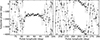 |
Fig. A.7. Sub-pulse phase tracks of MP (left) and IP (right) of PSR J1842+0358 computed at a P3 periodicity around 112. The two panels presents the sub-pulse phases with error bars, and with an arbitrary phase values in the vertical direction. |
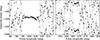 |
Fig. A.8. Sub-pulse phase tracks of MP (left) and IP (right) of PSR J1926+0737 computed at a P3 periodicity around 180. See caption of Fig. A.7 for more details. |
All Figures
|
Fig. 1. Main pulse (left) and interpulse (right) pulse stacks of PSR J1842+0358 from the MeerKAT observation. The pulse sequences are averaged over ten single pulses, but the pulse number on the y-axis still denotes the single-pulse number. The corresponding average profiles of all single pulses are shown in the top panels. |
| In the text | |
|
Fig. 2. Average pulse profile of PSR J1842+0358 from the FAST data for MP (left) and IP (right). The total intensity profile (normalised by the MP peak) is shown in black, and linear and circular polarisation are plotted in red and blue, respectively. The bottom panels show the PAs of the on-pulse regions. |
| In the text | |
|
Fig. 3. First 1000 single pulses for PSR J1842+0358. Pulse stacks (MP, IP) and intensities (single-pulse, running-averaged). Panel a: Pulse stack of the MP. The blue and green margin bars mark the bright pulses, based on the intensities of the single pulses (blue, left) or their running averages (green, right). Panel b: Same as (a) but for the IP, now with violet and brown for single-pulse or running-averaged intensities, respectively. Panel c: Single-pulse intensities of the MP and the IP, with the running averaged intensities plotted on top. Margin bars are identical to the left of (a) and (b). Panel d: Running averaged intensities of the MP and the IP plotted alone, along with the corresponding selected bars (the same as those on the right of a and b). The rest of the PSR J1842+0358 pulse stacks are available online. |
| In the text | |
|
Fig. 4. Pulse energy distributions of PSR J1842+0358 for MP (left) and IP (right), with single-pulse energies (blue and violet) and running-averaged pulse energies (green and brown). The same colours of the pulse energies corresponding to the bright groups as in Fig. 3 apply. The weak pulse energy distributions use the same but lighter set of colours. The two pulse energies are normalised by the mean MP energy. The vertical line indicates the cut of the two groups, of 1/3 bright and 2/3 weak pulse intensities (as described in Sect. 3.4.1). |
| In the text | |
|
Fig. 5. Average pulse profiles of MP and IP of PSR J1842+0358 based on the weakest and strongest groups of running-averaged pulses from the other pulse. Panel a: MP profiles based on, from top to bottom: weakest IP in running averaged (dark red), then brightest IP in running averaged (brown) marked in Fig. 4b. Panel b: IP average pulse profiles of the weakest and brightest groups of the MP, with colours in cyan and green, marked in Fig. 4a. |
| In the text | |
|
Fig. 6. Fluctuation spectra of PSR J1842+0358 for MP (left) and IP (right). Top: Average pulse profile and the modulation index (black dots with error bars) against pulse longitude. Middle: LRFS as fluctuation frequency (1/P3, in cycles per period, cpp). Its side panel shows the integrated power. Bottom: 2DFS, with fluctuation frequencies on both axes in cpp, with 1/P3 vs. 1/P2. Its left and bottom subpanels show the horizontal and vertical integrated power. The orange curve is the horizontal mirror image of the black curve in the bottom panel, indicating whether there are any possible drift in the pulse stack. The greyscale bars indicates the scale. Values above 1 are clipped. |
| In the text | |
|
Fig. 7. Correlation plots of PSR J1842+0358. Panel a: Auto-correlation curves of the MP and the IP intensities, which reveal the periodicities in the pulse intensities. The plots are zoomed in to the y-range of −0.2 to 0.4. Panel b: Cross-correlation between the MP and the IP single-pulse intensities and its error bars in black line, and the correlation when reversing the order of the single pulses in grey dashed line. The corresponding correlation of the off-pulse regions is in red. Panel c: Correlation plots computed using the running averaged intensities of the MP and the IP, with the FAST sequence in black, and the MeerKAT sequence in blue, respectively. |
| In the text | |
|
Fig. 8. Main pulse (left) and interpulse (right) pulse stacks of PSR J1926+0737. The pulse sequences were averaged over ten single pulses but the pulse number shows the number of single pulses. The corresponding average profiles of all single pulses are shown on the top panels. |
| In the text | |
|
Fig. 9. Average pulse profile of PSR J1926+0737 (top) for MP (left) and IP (right). The total intensity profile (normalised by the MP peak) is in black, and the corresponding linear and circular polarisation are shown in red and blue, respectively. The bottom plots show the computed polarisation position angles. |
| In the text | |
|
Fig. 10. First 1000 single pulses for PSR J1926+0737. Pulse stacks (MP, IP) and intensities (single-pulse, running average). Panel a: Pulse stack of the MP. The blue and green margin bars mark the bright pulses, based on the intensities of the single pulses (blue, left) or their running averages (green, right). Panel b: Same as (a) but for the IP, now with violet and brown for single-pulse and running-averaged intensities, respectively. Panel c: Single-pulse intensities of the MP and the IP, with the running averaged intensities plotted on top. Margin bars identical to the left of (a) and (b). Panel d: Running averaged intensities of the MP and the IP plotted alone, along with the corresponding selected bars (the same as those on the right of a and b). The rest of the PSR J1926+0737 pulse stacks are available online. |
| In the text | |
|
Fig. 11. Pulse energy distributions of PSR J1926+0737 for MP (left) and IP (right), with single-pulse energies (blue and violet) and running-averaged pulse energies (green and brown). Both pulse energies are normalised by the mean MP energy. The vertical line shows two groups that are split at the median pulse intensity (as described in Sect. 4.4.1). |
| In the text | |
|
Fig. 12. Average profiles of MP and IP of PSR J1926+0737 based on grouping pulses by the brightest and weakest halves of the opposite pulse. Panel a: MP profiles based on, from top to bottom: weakest IP in running averaged (dark red), then brightest IP in running averaged (brown) marked in Fig. 11b. Panel b: IP average pulse profiles, based on the MP halves, with colours in cyan and green, as marked in Fig. 11a. An anti-correlation is clearly present. |
| In the text | |
|
Fig. 13. Fluctuation spectra of PSR J1926+0737 for MP (left) and IP (right). For a full description, see Fig. 6. |
| In the text | |
|
Fig. 14. Correlation plots of PSR J1926+0737. Panel a: Auto-correlation curves of the MP and the IP intensities, which reveal any periodicities in the pulse intensities. The plots are zoomed-in to the y-range of −0.1 to 0.2. Panel b: Cross-correlation between the MP and the IP single-pulse intensities and its error bars in black line, and the correlation when reversing the order of the single pulses in grey dashed line. The corresponding correlation of the off-pulse regions is in red. Panel c: Correlation plots computed using the running averaged intensities of the MP and the IP, with the Fast full sequence in black, and the MeerKAT full sequence in blue, respectively. |
| In the text | |
|
Fig. 15. Left: Simulated pulse-intensity sequence within two P3 cycles of MP (blue) and IP (green) obtained as the average of selected single pulses (see text for details). Right: Corresponding cross-correlation curve. |
| In the text | |
|
Fig. A.1. Average pulse profiles of MP and IP of PSR J1842+0358 based on groups of pulses with different intensities. Panel a: MP peak-normalised average profiles of the bright and weak single-pulse intensities (blue and light blue) and running-averaged intensities (green and cyan), respectively. The average profile in black is also shown. Panel b: Same as (a) but IP peak-normalised average profiles, single-pulse intensities in violet and pink, and running averaged intensities in brown and dark red, respectively. Panel c: MP averaged profiles based on the weakest (dotted) and brightest (dashed) groups of single-pulse intensities and the running averaged intensities of the IP. Colours corresponds to the IP colours in (b). Panel d: Same as (c) but for the IP averaged profiles based on the two groups of the MP. Panels e and f: Same as (c) and (d) but now peak-normalised. |
| In the text | |
|
Fig. A.2. Average pulse profiles of MP (first column) and IP (second column) of PSR J1926+0737 based on groups of pulses with different intensities. See the caption of Fig. A.1 for details of each panel. |
| In the text | |
|
Fig. A.3. Longitude-resolved correlation map of PSR J1842+0358 at zero phase delay, and only the selected on-pulse regions are shown (note that the pulse longitudes are not consecutive, where the off-pulse regions are removed). The colour plot shows the corresponding cross correlations along pairs of pulse longitude. The side and bottom panels are the normalised integrated pulse profiles, with the dashed lines indicate boundary of the MP and the IP. |
| In the text | |
|
Fig. A.4. Longitude-resolved correlation map of PSR J1842+0358 at zero phase delay using the MeerKAT ten-pulse averaged data. Layout otherwise as Fig. A.3. |
| In the text | |
|
Fig. A.5. Longitude-resolved correlation map of PSR J1926+0737 at zero phase delay. Layout otherwise as Fig. A.3. |
| In the text | |
|
Fig. A.6. Longitude-resolved correlation map of PSR J1926+0737 at zero lag using the MeerKAT ten-pulse averaged data. See the caption of Fig. A.2 for further details. |
| In the text | |
|
Fig. A.7. Sub-pulse phase tracks of MP (left) and IP (right) of PSR J1842+0358 computed at a P3 periodicity around 112. The two panels presents the sub-pulse phases with error bars, and with an arbitrary phase values in the vertical direction. |
| In the text | |
|
Fig. A.8. Sub-pulse phase tracks of MP (left) and IP (right) of PSR J1926+0737 computed at a P3 periodicity around 180. See caption of Fig. A.7 for more details. |
| In the text | |
Current usage metrics show cumulative count of Article Views (full-text article views including HTML views, PDF and ePub downloads, according to the available data) and Abstracts Views on Vision4Press platform.
Data correspond to usage on the plateform after 2015. The current usage metrics is available 48-96 hours after online publication and is updated daily on week days.
Initial download of the metrics may take a while.