| Issue |
A&A
Volume 706, February 2026
|
|
|---|---|---|
| Article Number | A111 | |
| Number of page(s) | 11 | |
| Section | Extragalactic astronomy | |
| DOI | https://doi.org/10.1051/0004-6361/202556307 | |
| Published online | 03 February 2026 | |
Investigating the influence of radio-faint active galactic nuclei on the infrared-radio correlation of massive galaxies
1
INAF – Osservatorio di Astrofisica e Scienza dello Spazio di Bologna Via Gobetti 93/3 I–40129 Bologna, Italy
2
Jodrell Bank Centre for Astrophysics, University of Manchester Oxford Road Manchester M13 9PL, UK
3
Department of Physics, University of Pretoria Lynnwood Rd Hatfield Pretoria 0002, South Africa
4
CEA, Universitè Paris-Saclay, Université Paris Citè, CNRS, AIM 91191 Gif–sur–Yvette, France
5
University of the Witwatersrand Enoch Sontonga Ave Johannesburg, South Africa
6
University of Birmingham Birmingham B15 2TT, United Kingdom
7
INAF – Istituto di Radioastronomia Via Gobetti 101 I–40129 Bologna, Italy
8
Dipartimento di Fisica e Astronomia (DIFA), Università di Bologna Via Gobetti 93/2 I-40129 Bologna, Italy
9
Institute of Physics, Laboratory of Astrophysics, École Polytechnique Fédérale de Lausanne (EPFL) 1290 Sauverny, Switzerland
10
Department of Physics, University of Zagreb Bijenička Cesta 32 Zagreb, Croatia
11
Caltech/IPAC 1200 E. California Blvd. Pasadena CA 91125, USA
12
University of Western Australia 35 Stirling Hwy Crawley WA 6009, Australia
13
Cosmic Dawn Center (DAWN), Denmark
14
DTU Space, Technical University of Denmark Elektrovej 327 2800 Kgs. Lyngby, Denmark
15
Swinburne University of Technology John Street Hawthorn Victoria 3122, Australia
★ Corresponding authors: This email address is being protected from spambots. You need JavaScript enabled to view it.
; This email address is being protected from spambots. You need JavaScript enabled to view it.
Received:
8
July
2025
Accepted:
3
October
2025
Abstract
Context. It is well known that star-forming galaxies (SFGs) exhibit a tight correlation between their radio and infrared emissions, commonly referred to as the infrared-radio correlation (IRRC). Recent empirical studies have reported a dependence of the IRRC on the galaxy stellar mass, in which more massive galaxies tend to show lower infrared-to-radio ratios (qIR) with respect to less massive galaxies. One possible, yet unexplored, explanation is a residual contamination of the radio emission from active galactic nuclei (AGNs), not captured through “radio-excess” diagnostics.
Aims. To investigate this hypothesis, we aim to statistically quantify the contribution of AGN emission to the radio luminosities of SFGs located within the scatter of the IRRC.
Methods. Our Very Large Baseline Array (VLBA) AGN-sCAN program has targeted 500 galaxies that follow the qIR distribution of the IRRC, i.e., with no prior evidence for radio-excess AGN emission based on low-resolution (∼arcsec) VLA radio imaging. Our VLBA 1.4 GHz observations reach a 5σ sensitivity limit of 25 μJy/beam, corresponding to a radio-brightness temperature of Tb ∼ 105 K. This classification serves as a robust AGN diagnostic, regardless of the host galaxy’s star formation rate.
Results. We detect four VLBA sources in the deepest regions, which are also the faintest VLBI-detected AGNs in SFGs to date. The effective AGN detection rate is 9%, when considering a control sample matched in mass and sensitivity, which is in good agreement with the extrapolation of previous radio AGN number counts. Despite the non-negligible AGN flux contamination (∼30%) in our individual VLBA detections, we find that the peak of the qIR distribution is completely unaffected by this correction. Although we cannot rule out a high incidence of radio-silent AGNs at (sub)μJy levels among the VLBA non-detections, we derive a conservative upper limit of < 0.1 dex of their cumulative impact on the qIR distribution. We conclude that residual AGN contamination from non-radio-excess AGNs is unlikely to be the primary driver of the M★ – dependent IRRC.
Key words: instrumentation: interferometers / surveys / galaxies: active / galaxies: nuclei / galaxies: star formation
© The Authors 2026
 Open Access article, published by EDP Sciences, under the terms of the Creative Commons Attribution License (https://creativecommons.org/licenses/by/4.0), which permits unrestricted use, distribution, and reproduction in any medium, provided the original work is properly cited.
This article is published in open access under the Subscribe to Open model. This email address is being protected from spambots. You need JavaScript enabled to view it. to support open access publication.
1. Introduction
Star-forming galaxies show a positive relation between total infrared (IR) luminosity (LIR, rest-frame 8−1000 μm) and monochromatic radio luminosity (e.g., at 1.4 GHz; L1.4), which remains remarkably tight (σ ∼ 0.26 dex; e.g., Bell 2003) and linear for over three orders of magnitude in both LIR and L1.4 GHz (e.g., Helou & Rowan-Robinson 1985; Condon 1992, even though a mild nonlinearity was also found in low-z galaxies, e.g., at z < 0.2 Molnár et al. 2021). This is generally known as the infrared-radio correlation (IRRC). The origin of the IRRC arises from the relationship between radio luminosity and (obscured) star formation rate (SFR). Broadly speaking, the IR emission arises from the light of massive OB stars, which is absorbed and re-emitted by dust (Madau & Dickinson 2014) and therefore directly traces the galaxy’s SFR. On the other side, radio-continuum emission at GHz frequencies originates mainly from synchrotron processes, produced by relativistic cosmic-ray electrons (CRe) accelerated by shock waves produced when massive stars (> 8 M⊙) explode as supernovae, in the case of star-forming galaxies (SFG).
The logarithmic ratio between the two luminosities, labelled qIR, is defined as
![Mathematical equation: $$ \begin{aligned} q_{\rm IR} = {\log \left(\frac{L_{\rm IR}\,\mathrm{[W]}}{3.75 \times 10^{12}\,\mathrm{[Hz]}}\right) - \log (L_{1.4\,\mathrm{GHz}}\,\mathrm{[W/Hz]})}, \end{aligned} $$](/articles/aa/full_html/2026/02/aa56307-25/aa56307-25-eq1.gif) (1)
(1)
where 3.75 × 10¹² Hz represents the central frequency over the far-infrared (e.g., 42−122 μm) regime. However, the nature of the cosmic evolution of the IRRC has long been debated (e.g., Harwit & Pacini 1975; Rickard & Harvey 1984; de Jong et al. 1985; Helou & Rowan-Robinson 1985; Hummel et al. 1988; Condon 1992; Garrett 2002; Appleton et al. 2004; Jarvis et al. 2010; Sargent et al. 2010; Ivison et al. 2010a,b; Bourne et al. 2011; Magnelli et al. 2015; Delhaize et al. 2017; Gürkan et al. 2018; Molnár et al. 2018; Algera et al. 2020; Basu et al. 2015; Rivera et al. 2017).
Several studies (Magnelli et al. 2015; Rivera et al. 2017; Delhaize et al. 2017) observed a dependence of the IRRC on the redshift, in the form of qIR ∝ (1 + z)δ with −0.1 < δ < −0.2. Other works (Gürkan et al. 2018; Smith et al. 2021; Delvecchio et al. 2021, D21 hereafter) have recently argued that the IRRC evolves primarily with M★, with more massive galaxies showing a systematically lower qIR, while the dependence on the redshift is secondary and weaker, as qIR ∝ (1 + z)−0.023 ± 0.008 at a fixed stellar mass (see also Gürkan et al. 2018; Smith et al. 2021). Among the possible physical drivers of the qIR decline observed in massive star-forming galaxies, the energy loss of cosmic-ray electrons (CRes) has been suggested to play a significant role (e.g., Schober et al. 2023; Yoon 2024). Specifically, Yoon (2024) modeled the CRe energy-loss as a function of the gas density and redshift of the host galaxy. Their findings indicate an anticorrelation between these quantities; specifically, galaxies with higher gas densities (or, equivalently, higher stellar masses; e.g., Kennicutt 1998) experience less intense energy losses, arguably because they retain their CRes more easily. On the contrary, less massive galaxies are generally most affected by CRe energy losses. As a consequence of these synchrotron energy losses, less massive galaxies have lower radio luminosities with respect to more massive ones.
One yet unexplored explanation for the M★ evolution is that a hidden and widespread contribution from radio AGN activity might be driving the decline of the qIR, especially at high stellar masses (log(M★/M⊙)≥10). One very powerful tool to assess the nature of radio emission is the brightness temperature of the emitter (Tb), defined as
![Mathematical equation: $$ \begin{aligned} T_b\,\mathrm{[K]} = 1.22 \times 10^6 \times (1+z) \times \left(\frac{{S\!}_{\rm obs}}{\upmu \mathrm{Jy}}\right) \left(\frac{\nu }{\mathrm{GHz}}\right)^{-2} \left(\frac{\theta _x \cdot \theta _y}{\mathrm{mas}^2}\right)^{-1}, \end{aligned} $$](/articles/aa/full_html/2026/02/aa56307-25/aa56307-25-eq2.gif) (2)
(2)
where Sobs is the observed density flux at the frequency ν, and θx and θy are the major and minor axes of the beam (Ulvestad et al. 2005).
Traditionally, high Tb measurements (Tb ≥ 105 K) require very long baseline interferometry (VLBI), which reaches milliarcsecond resolutions at GHz frequencies (e.g., Middelberg et al. 2010, 2013; Rampadarath et al. 2015; Herrera-Ruiz et al. 2017, 2018; Radcliffe et al. 2018, 2021; Njeri et al. 2023; Deane et al. 2024). Recent studies performed with the Very Long Baseline Array (VLBA) at a few milliarcsecond (mas) resolution (e.g., 10 mas ∼ 80 pc at z = 2) have identified AGNs even in galaxies whose emission is dominated by star formation at Very Large Array (VLA) scales (Herrera-Ruiz et al. 2017, 2018; Maini 2017). However, these pioneering studies have been highly biased toward radio-excess AGNs (i.e., showing excess radio emission relative to that expected from pure star formation; Smolčić et al. 2017). Our project AGN-sCAN extends this type of analysis by targeting with the VLBA a representative sample of SFGs without strong VLA radio-excess, down to a sensitivity reaching as deep as σ ≈ 5 μJy/beam at 1.4 GHz at high angular resolution (average beam size: 26 × 7 mas2). From Eq. (2), the Tb limit at > 5σ for an unresolved source at z = 0.5 is Tb ≥ 105 K1. Compact radio cores (∼mas scales) characterized by such Tb would unambiguously arise from an AGN (Condon 1992; Radcliffe et al. 2018; Morabito et al. 2022).
Section 2 describes the main physical properties of the radio targets composing the sample used in this work. Section 3 summarizes the AGN-sCAN observational strategy and data products, of which a complete and detailed description will be presented by Delvecchio et al. (in prep., D26 hereafter). Section 5 summarizes our main result: the contribution of AGN emission to the nuclear emission of SFGs, classified through the IRRC, is negligible.
We adopted a Chabrier (2003) initial mass function in the mass range 0.1−100 M⊙. We assumed a standard ΛCDM cosmology with Ωm = 0.3, ΩΛ = 0.7, and H0 = 70 km s−1 Mpc−1. We defined the radio spectral index, α, with the following convention: Sν ∝ ν−α, where Sν is the flux density at a frequency, ν.
2. Sample selection and physical properties
This VLBA program (ID: VLBA/20B-140, PI: Delvecchio) has targeted 500 massive (M★ ≥ 1010 M⊙) star-forming galaxies in the Cosmic Evolution Survey (COSMOS; Scoville et al. 2007), which is an equatorial 2 deg2 field observed with all major space- and ground-based telescopes2. We refer the reader to D26 for the detailed description of the survey.
The parent galaxy sample was retrieved from the COSMOS-Web survey (Casey et al. 2023), containing deep imaging in four JWST/NIRCam filters (F115W, F150W, F277W, F444W) over 0.54 deg2 (Franco et al. 2025), and with JWST/MIRI 7.7 μm over 0.2 deg2 (Harish et al. 2025). Given that our VLBA pointing lies within the COSMOS-Web NIRCam footprint, we updated all redshifts and counterpart properties from the latest COSMOS-Web photometric catalogue (Shuntov et al. 2025), which extends in wavelength out to Spitzer-IRAC bands. Photometric redshifts are in very good agreement with spectroscopic measurements (i.e., median absolute deviation σMAD ∼ 0.012 at mF444W < 28; see Khostovan et al. 2026). We adopted the spectroscopic measurement if available and reliable (> 95% confidence level) based on the compilation by Khostovan et al. (2026).
In order to retrieve a qIR measurement for each target, we require our galaxies to have been detected (≥5σ) at both IR and radio frequencies. The combined IR dataset comes from de-blended far-infrared/sub-mm data from Herschel (100−500 μm), SCUBA2 (450, 850 μm), AzTEC-1.1 mm, MAMBO-1.2 mm (Jin et al. 2018), and ALMA from the recent A3COSMOS survey (Liu et al. 2019; Adscheid et al. 2024), whenever available. For each source, the total IR luminosity (8−1000 μm, LIR) is obtained via spectral energy distribution (SED) fitting, and corrected for potential IR-AGN emission (Jin et al. 2018). Radio counterparts are jointly taken from MIGHTEE 1.28 GHz (6″ resolution, Jarvis et al. 2016; Heywood et al. 2022), VLA 1.4 GHz (1.5″ resolution, Schinnerer et al. 2010), and VLA 3 GHz (0.75″ resolution, Smolčić et al. 2017) imaging. The rest-frame 1.4 GHz luminosity (L1.4) is derived from the radio dataset with the highest available signal-to-noise (S/N), and K-corrected to the 1.4 GHz rest frame by assuming a power-law spectrum with a spectral index, α, between 3 GHz and 1.28/1.4 GHz, or assuming α = 0.75 if not jointly detected. To match the spatial resolutions between the 3 GHz and 1.4 GHz images, we downgraded the 3 GHz map by convolving it with a Gaussian kernel of 1.5″ full width at half maximum (FWHM) (similarly to, e.g., Gim et al. 2019). We refrained from using a larger FWHM (i.e., for 1.28 GHz counterparts from MeerKAT), as Delhaize et al. (2017) showed that the flux increase above 1.5″ is typically negligible. The new 3 GHz fluxes at 1.5″ resolution are higher by 6%, on average, compared to those of the native resolution (0.75″) map. This effect induced a minimal flattening in the re-calculated spectral index for the joint 1.4−3 GHz detections (for a in-depth discussion about the influence of the radio spectral index on the IRRC, see Sect. 4.4.1 in Delhaize et al. 2017).
As for the IR part, we required the combined S/N (summed in quadrature over all Herschel, SCUBA2, AzTEC, and ALMA bands) be higher than five. For the same reason, for the radio part, we required the 1.4 GHz flux to be higher than 25 μJy; that is, 5× the VLBA 1.4 GHz sensitivity at the pointing center. We restricted ourselves to galaxies at z> 0.5 in order to obtain the full galaxy size within the VLBA field of view limited by bandwidth smearing (i.e., 5.5″ diameter). We disregarded all previously detected VLBA targets from Herrera-Ruiz et al. (2017, 2018) to avoid duplications.
These selection criteria naturally identify 500 massive (M★ ≳ 1010 M⊙) galaxies. This sample is representative of star-forming galaxies on the IRRC, as they are broadly distributed in qIR around the (M★, z)-dependent IRRC from Delvecchio et al. (2021) (see also Sect. 5 for details).
3. Observation and data calibration
Our VLBA observations are summarized in the following, while further details are given in D26. In each VLBA session, the full L-band bandwidth is split into eight spectral windows of 32 MHz each, further divided into 16 spectral channels (2 MHz each) at 4 s time resolutions. This setup yields a field of view limited by a time (bandwidth) smearing of 10.82″ (2.75″), which is hence larger than the typical galaxy size at z > 0.5 (Yang et al. 2025). The final images of all targets, consisting of 4096 × 4096 pixels (at 0.001″/px scale) weighing about 67 Mbyte each3.
The pointing center was located at RA (J2000) = 10:00:36.3299 and Dec (J2000) = +02:12:58.773 and covers 30′ FWHM at 1.4 GHz. It was observed for a total of 120 h, split into 24 epochs of 5 h each, due to the limited visibility of COSMOS by all ten VLBA antennas for longer tracks. Raw data were calibrated using the VLBI PIPEline (VPIPE; Radcliffe et al. 2024, and in prep.4) that is designed to perform automated instrumental calibration, phase referencing, and imaging for multiphase center VLBI observations. All these steps have been successfully tested in former very long baseline surveys (EVN from Radcliffe et al. 2018, 2021; VLBA from Deane et al. 2024).
In order to evaluate the significance of each VLBA source as a function of the peak S/N, we ran simulations using the Common Astronomy Software Applications (CASA, v.6.6) package. We refer the reader to D26 for more technical details on this task. Briefly, we considered the real noise map, taken from an empty sky region at the VLBA pointing centre, and injected one point-like source in the uv-plane, with known position and S/N. We iterated the simulation 100 times, keeping the input position fixed, but varying the input S/N over the 4.5 ≤ S/N ≤ 7.5 range. Only one source was injected into each realization in order to mitigate side-lobe effects and obtain reliable output fluxes. We then imaged each simulated dataset, adopting the same setup used for real data and employing BLOBCAT (Hales et al. 2012) to extract the flux and position of all blobs above a given peak S/N in each image. While the completeness at S/N > 4.5 is always observed to be higher than 90% (i.e., BLOBCAT finds the one input source in > 90% of runs), the fraction of spurious blobs is a strong function of the S/N. In particular, we defined the “spuriousness” (pspur) as
 (3)
(3)
where Ninp is the number of “real” (input) blobs and Nout is the number of the (output) detected blobs. We counted the output blobs within a radius of ±0.2″ from the input (real) source, similarly to what we did for real detections (see Sect. 4). We find that the spuriousness is higher than 50% at S/N < 5, while it decreases to ≈15% at S/N ∼ 5.5, and it exponentially drops below 2% at S/N ≥ 6. If counting all random blobs over the full image (4″ × 4″), the spuriousness at a fixed S/N increases proportionally to the searching area, except at S/N > 6 where it drops to below 2% as found in the central area.
4. Final sample of VLBA detections
Following Herrera-Ruiz et al. (2017) (HR2017 hereafter), we obtain the total fluxes from BLOBCAT (Hales et al. 2012) by integrating the blobs with S/N ≥ 5.5 that are found within ±0.2″; that is, ±1 VLA 3 GHz pixel from the prior VLA counterpart position (Smolčić et al. 2017), which sets our maximum VLBA-VLA separation – in HR2017 it was ±0.4″, i.e., ±1 VLA 1.4 GHz pixel (Schinnerer et al. 2010). For consistency, our chosen size of ±0.2″ is also the circular region inside which we forced the cleaning in order to maximize the S/N. Based on the above criteria, we identified four VLBA detections associated with AGN activity, with their main properties listed in Table 1. We also show them in Fig. 1, where the presence of a compact radio core is evident (e.g., purple contours). The average VLBA rms of these four detections is 6 μJy/beam. Interestingly, these sources are the faintest AGNs ever detected with VLBI techniques in SFGs. If pushing our detections threshold to a lower S/N, in particular at 5.0 < S/N < 5.5, we would identify two additional source candidates, but their high spuriousness (∼40% at their average S/N ∼ 5.2) does not allow us to claim them as secure detections.
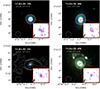 |
Fig. 1. RGB images of targets VLBA ID ‘338’ (top left), ‘351’ (top right), ‘408’ (bottom left), and ‘498’ (bottom right). These were obtained by combining the F150W, F277W, and F444W JWST/NIRCam filters (Franco et al. 2025) covering a 5″ × 5″ field of view. The NIRCam pixel scale is 30 mas. The white contours are the VLA 3 GHz levels (Smolčić et al. 2017) at three, four, five, and six times the rms (2.3 μJy/beam; the VLA beam size is 0.75″ as shown by the white circle in the bottom left). In the zoomed-in images of the red panels, the purple contours are the levels at two, three, four, five, and six times the image rms detected by the VLBA, which come from a 0.2″ × 0.2″ field of view (also outlined by the red square at the centers of the galaxies). The dotted purple contour also shows the −3 rms level. The VLBA beam size for each detection is: 26 × 5 mas2 (‘338’), 26 × 5 mas2 (‘351’), 28 × 5 mas2 (‘408’), and 23 × 6 mas2 (‘498’), with a similar position angle PA ∼ 162°. |
Summary of the four VLBA-AGN’s properties.
We note in Fig. 1 that the VLBA (iso-surface brightness) contours appear more complex than the elongated synthesized beam. This is because three out of four detections (all but 498) are marginally resolved (along the beam minor axis) according to BLOBCAT (Hales et al. 2012). However, given the low S/N of these detections, the limited uv coverage and the lack of a priori information on the source morphology, the imaging and deconvolution process becomes highly uncertain (e.g., Taylor et al. 1999). In such conditions, the final restored contours can be a complex blend of different spatial components and are not expected to strictly follow the shape of the clean beam; hence, some contours of faint sources would appear rounder and/or smaller than the synthesized beam. This is a known issue in deep VLBI imaging and has been observed in other VLBI surveys (e.g., Radcliffe et al. 2018). Because the three resolved detections display non-Gaussian morphologies, as recommended in Hales et al. (2012) we took total VLBA fluxes (e.g., SVLBA in Table 1) from the corresponding observed integrated values, but skipping the Gaussian volume correction. For the only unresolved detection (498) we instead set the total flux equal to the peak flux.
In order to make a fair comparison between our VLBA detections and non-detections, we define two control samples of VLBA non-detections (CS hereafter): (i) a M★-matched CS (i.e., with log (M★/M⊙) > 10.5; 277 objects) and a combined [M★, rms]-matched CS (i.e., a subset of the first CS, also with rms < 6.7 μJy beam−1; i.e., the highest among the four detections; 42 objects). Therefore, this latter CS contains the VLBA targets that were not detected within a depth-matched area, despite them being equally as accessible as for the VLBA detections. Overall, the effective detection rate in our sample is 9% (i.e., 4/46), which is broadly consistent with the AGN duty cycle in massive star-forming galaxies (Delvecchio et al. 2022; Wang et al. 2022). We note that matching the control sample by the lowest or average rms of the detections would not have changed the effective detection rate.
5. The AGN-corrected infrared-to-1.4 GHz radio luminosity ratio
We measured qIR exploiting the total radio VLA luminosities, where both star formation and AGN activity can, in principle, contribute. Figure 2 shows these values as a function of the stellar mass of the host galaxy. Dark stars mark the four detections, the light blue circles indicate the M★-matched CS, while the darker blue circles represent the (M★, rms)-matched CS. The solid black line represents the dependence of the IRRC on the stellar mass for galaxies at a ⟨z⟩∼1, as indicated by the relationship described by Delvecchio et al. (2021):
 (4)
(4)
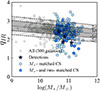 |
Fig. 2. qIR distribution as function of host galaxy stellar mass for all 500 targets (gray points), four VLBA-detected AGNs (blue stars), and 277 non-detections part of the M★-matched sample (light blue points). The qIR of the detections account for the AGN emission detected by the VLBA (e.g., qIR, corr). The darker blue points are the 42 non-detections observed at sensitivities equal to or lower than the sensitivity of the detections, thus constituting the (M*, rms)- matched CS. The black line is the qIR versus log M★/M⊙ relation from Delvecchio et al. (2021) at ⟨z⟩∼1, and the shaded areas span the scatter of the IRRC at M★ > 1010.5 M⊙ from Delvecchio et al. (2021), of around ±0.22 dex and ±0.44 dex. |
where A = (1 + z) and B = log(M★/M⊙).
It is important to note that the dependence on the stellar mass is stronger than that with the redshift. To measure the qIR(M★, z), we considered the stellar masses and redshifts presented in Sect. 3. Since the qIR(M★, z) distributions are similar between the M★- and (M★, rms) – matched CS (as expected given that the observed qIR does not depend on the VLBA rms), in the following we consider the qIR(M★, z) distribution of the M★-matched CS to increase the statistics.
If we assume that the incidence of AGNs is as high as in the deepest regions across the entire sky area mapped by the AGN-sCAN survey, we can then reason that the number of effective detections would have been seven times greater than the NAGN = 4 detected in regions with an rms < 6.7 μJy/beam. This factor of seven was determined by noting that the subset of non-detections matched on both stellar mass and rms, (M★, rms)-CS, is approximately seven times smaller than the subset matched solely by stellar mass (e.g., M★-CS).
Next, we measured the difference (ΔqIR) between qIR(M★, z) and the observed qIR computed using the VLA luminosities in Eq. (1). In the left panel of Fig. 3, the light purple histogram displays the distribution of ΔqIR for the (M★, rms)-CS, while the dark purple histogram displays the distribution of ΔqIR for the detections. To reproduce the expected IRRC for pure SFGs, we built up the so-called mirror distribution (dashed orange histogram). This is obtained by mirroring the right side of the real distributions, assumed to be purely originating from SF processes, onto the left side. The errors associated with the counts of the mirror distributions (orange shaded area) were calculated with a bootstrap by extracting 1000 values from a Gaussian distribution centered on the observed number counts (N), in each bin, with a standard deviation of  . We observe that the mirror distribution peaks around zero in both panels. This allowed us to visually assess how much the observed distribution deviates from a perfect Gaussian. In the right-hand panel of Fig. 3, we instead plot the distributions of the difference between qIR(M★, z) and the corrected qIR (qIR, corr), after subtracting the AGN emission observed with the VLBA. In this case, ΔqIR, corr equals log[(LVLA)/(LVLA − LVLBA)], which is > 0 by definition.
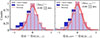 |
Fig. 3. Normalized distributions of difference between the observed qIR and the one expected from Eq. (4) (Delvecchio et al. 2021) based on the stellar mass and the redshift of the host galaxy, qIR (M★, z). The light purple histogram represents the distribution of the (M★, z)-CS. The stacked dark purple histogram (i.e., dark purple histogram on top of the light purple one) represents the detections, and the hatched orange histogram is the so-called mirror distribution, interpreted as the intrinsic qIR distribution of SFGs. The bootstrapped median values of the mirror distribution were fit with a Gaussian (red curve; see Sect. 5 for further details). Left panel: qIR was computed using the VLA luminosity coming from both star formation and AGN activity. Right panel: qIR, corr is measured after subtracting the AGN radio luminosity detected by the VLBA from the total radio VLA emission. |
The first thing to note is that the median values of the real distributions remain unchanged before and after the correction for the AGN contribution to the radio luminosities. Both before and after the correction, we estimate  dex. The errors on the median are calculated as the 16th and 84th percentiles of the distribution, divided by the square root of the total counts. However, it was expected that the AGN contribution would have a minimal impact on the scatter within the IRRC for these galaxies due to the low fraction of detections. Nevertheless, it is interesting to note that on an individual source basis, the AGN fluxes substantially influence qIR, since the average difference between qIR and qIR, corr for the detections is about 0.14 dex (e.g., 30%), which is not negligible.
To further explore the potential role of radio variability, we examined the list of variable 1.5 GHz sources identified in the CHILES VERDES survey (Sarbadhicary et al. 2021). The survey provides 1−2 GHz continuum VLA data obtained between 2013 and 2019 in a 0.44 deg2 area of the COSMOS field for 750 galaxies previously detected at VLA-1.4 GHz. Moderate variability (10−30% flux density variation) was observed in 18 sources, and low-variability (2−10% flux density variation) in 40 sources, for a total of 58/750 (6%) variable targets. Only one of those variable sources is in common with our VLBA 1.4 GHz targets (even though it is not a VLBA detection) and exhibits low VLA variability (±5%). Moreover, based on the comparison between VLBA-1.4 GHz (Herrera-Ruiz et al. 2017) and VLA-1.4 GHz (Schinnerer et al. 2010) fluxes taken at different epochs (2012 vs 2007, respectively), Herrera-Ruiz et al. (2017) found 13/468 (∼3%) VLBA detections with VLBA flux higher than the total VLA flux (at above > ±1σ uncertainty), which the authors interpreted as possible sign of variability. However, those 13 sources all have Svlba > 200 μJy, making them among the brightest of their sample. Hence, we expect a negligible fraction of radio-variable sources among our even fainter targets.
We also find that the real distribution exhibits a deviation from the Gaussianity (e.g., when compared to the mirror distribution) on the left side in both panels. However, this is minimal, as a K-S test could not reject the hypothesis that these two distributions come from the same parent sample (with a p value of 0.997).
Finally, we note that the mirror distributions are basically unchanged even after correcting the qIR of the detections. Besides the peak, also their standard deviations are fully consistent (from σ = ±0.44 dex to σ = ±0.45 dex). Overall, these results highlight that VLBA AGN contamination, despite being non-negligible for individual detections, does not impact the peak position (and the overall shape) of the original qIR distribution at all.
For completeness, in Appendix A, we correct the values of qIR for the dependence on redshift. We also verified that in that case the distribution of the z-corrected qIR distribution remains unchanged before and after the AGN correction.
6. Source counts
Following a similar approach to Deane et al. (2024) and Herrera-Ruiz et al. (2018), we computed the differential source counts, dN/dSν, as a function of source 1.4 GHz flux density, Sν, using the expression
 (5)
(5)
where N is the number of sources in a flux-density bin, Ω is the area over which a source with flux density equal to the mean flux density of the bin could be detected, and ΔS is the width of the flux-density bin.
Figure 4 displays the 1.4 GHz source count of the VLBA-detected AGN presented in this work (red star). For comparison, we also show the differential source counts derived by Herrera-Ruiz et al. (2018) using the VLBA COSMOS survey (as black dots), the derived source counts for the VLBA CANDELS GOODS-North Survey from Deane et al. (2024) (as red circles), and the VLA 3 GHz source counts split into SF and AGN subpopulations from Novak et al. (2018). The Novak et al. (2018) curves were obtained by statistically separating SFGs and radio AGNs based on the “radio-excess” criterion (Delvecchio et al. 2017) using data from the VLA-COSMOS 3 GHz Large Project (Smolčić et al. 2017). Our results are perfectly consistent with these previous works, as indeed the VLBA source counts at S1.4 GHz = 37 − 58 μJy follow the red curve in Novak et al. (2018), which is representative of the AGN population. At these fluxes, the AGN number counts are ∼5× lower than those of the total radio source population. This corroborates that the average AGN fraction of ∼20% among sources within this flux regime, while ∼80% of the sources are SFGs.
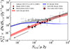 |
Fig. 4. Euclidean normalized radio-source number counts obtained by fitting with the Markov chain Monte Carlo algorithm, and the total radio luminosity function (LF) from Novak et al. (2018) using different evolving analytical LFs for AGN hosts (red line) and SF galaxies (blue line). The shaded areas encompass the 3σ errors from the χ2 fits performed on individual populations (for further details, see Novak et al. 2018). Gray circles are the number counts from Galluzzi et al. (2025) obtained from a compilation of radio observations with different instruments (e.g., VLA 1−3 GHz, ATCA, GMRT, LOFAR, MeerKAT, etc.), without any distinction between AGNs or SF. Red and black circles show the number counts from the VLBA CANDELS GOODS-North Survey (Deane et al. 2024) and VLBA 1.4 GHz COSMOS (Herrera-Ruiz et al. 2018) in the case of radio emission from AGN activity. The red star is the number count of the detections from the AGN-sCAN survey presented in this work. The gray arrow points toward the regime below our sensitivity limit, from which the number counts extrapolated from the red curve of Novak et al. (2018) of the 42 brightest AGN were extracted, in order to constrain upper limits on our results (see text in Sect. 7.1 for further details). |
Our measurement in Fig. 4 (red starred symbol) is the faintest source-count measurement ever obtained from VLBI studies, and it aligns well with previous (low-resolution) extrapolations of AGN number counts (solid red line). In this context, Whittam et al. (2017) hinted at a possible flattening of the AGN number counts toward faint flux densities, meaning that compact, flat-spectrum radio cores are increasingly dominant in these regimes. Although we do not have enough statistics to robustly test this hypothesis, we remark that the excess of flat-spectrum radio cores could indicate the presence of younger radio jets, short duty cycles, weak jet collimation, or slower jet speeds (for an in-depth discussion, see Deane et al. 2024).
7. Discussion
7.1. Cumulative distribution of AGNs in the faintest regime
Our 5.5σ sensitivity limit enabled us to detect AGN activity with flux densities down to ⟨S1.4⟩ = 37−58 μJy. Of course, we cannot rule out a widespread contribution of AGNs at even fainter fluxes. Unveiling those ultra-faint AGNs is, however, very challenging. VLBA stacking would improve our sensitivity limit, but it is not feasible due to to the lack of prior knowledge concerning AGN positions. The VLA peak flux position was indeed not sufficient to serve as a prior, as the VLBA has over ×10 higher spatial accuracy. Similarly, HST or JWST positions are significantly less accurate than VLBA positions, with the additional caveat that they could trace star formation, which might not be spatially coincident with AGN emission. Therefore, we attempted a statistical assessment of the AGN contamination in VLBA non-detections.
We derived a quantitative threshold of how faint the required flux limit would have to be, by conservatively assuming that our VLBA non-detections from the (M★, rms)-matched CS are the first 42 brightest AGNs expected just below the faintest flux of our VLBA detections; i.e., at S1.4 < 37 μJy. To do so, we converted the Euclidean-normalized 1.4 GHz source counts into a dimensionless quantity, re-scaled to the effective sky area of the (M★, rms)-matched CS (i.e., 9.7 × 10⁻⁶ sr). This yields a number of expected AGNs in the same area, as a function of 1.4 GHz flux. We made sure that the relation between differential NAGN and S1.4 yielded an integrated NAGN = 4 in the range 36−58 μJy (i.e., matching our VLBA detections; red star in Fig. 4). Then, we extrapolated the same trend down and below our nominal VLBA flux-density limit. Finally, we computed the cumulative distribution of NAGN at S1.4 < 37 μJy, and we found out that 42 sources would be cumulated at a flux density of 5 μJy, which is the minimum flux density reached by the ≈42 brightest AGNs. We stress again that this is an over-conservative assumption, since it is very unlikely that our non-detections are all clustered just below the flux limit. However, at these low flux densities, the brightness temperature drops to Tb ≪ 105 K (see Eq. (2)). This suggests that, even if we were able to detect such faint sources with the VLBA, the origin of their emission would be ambiguous between AGNs or star formation. Consequently, we conclude that pushing VLBA observation to sub-μJy sensitivity would not be an effective strategy for revealing a residual hidden population of radio AGNs. For instance, according to the ngVLA exposure time calculator5, we note that Band 1 (2.3 GHz observations) would reach brightness temperatures of Tb ≥ 105 K (at 5σ; i.e., ≈5μJy/beam) in about 16 h on source. Hence, fainter fluxes, as expected for the bulk of our VLBA non-detections, would be detected with a lower TB < 105 K, thus carrying an ambiguous origin despite their easy detection.
Furthermore, even in this conservative scenario in which our non-detections are the brightest AGNs below our sensitivity limit, the ratio SVLBA/SVLA is 17% at SVLA ≈ 70 μJy. SVLBA is the mean flux of the 42 brightest AGNs obtained from the cumulative distribution of the AGN number counts in the 5 μJy ≤ S1.4 ≤ 36 μJy range, while SVLA is the mean VLA 1.4 GHz flux density of the 42 non-detections. This ratio would translate into a global upper qIR shift of < 0.1 dex. We note that, based on the M★-dependent IRRC, qIR decreases by 0.22 dex within the same M★ range of the analysed sample (log M★/M⊙ > 10.5, Delvecchio et al. 2021). Therefore, given that radio AGN contamination (including VLBA detections and non-detections) counteracts this effect by < 0.1 dex, the decreasing qIR with M★ is not primarily explained by AGN contamination.
Among other possible mechanisms that have been proposed to explain the decline of qIR at stellar masses log(M★/M⊙)≥10.5 in SFGs, there is an increasing energy-loss rate of high-energy CR electrons, which can be due to particularly efficient supernova-driven turbulence (Schober et al. 2023). The CR energy loss could also depend on the gas surface density and the redshift of the host galaxy, as modeled by Yoon (2024). Finally, Ponnada et al. (2025) found that in many cases “radio-excess” objects can be better understood as “IR-dimmed” objects with longer-lived radio contributions at low-z from Type-Ia supernovae and intermittent black-hole accretion in weak SFGs.
7.2. Diffuse AGN emission as a possible caveat
A potential caveat of this analysis is that the AGN flux could be underestimated because of extended emission (beyond the VLBA beam; e.g., 200 pc × 50 pc at z = 1), that is resolved out by the VLBA (e.g., Morabito et al. 2025). We first tested that the integrated fluxes remain consistent across various tapering and Briggs schemes in our images. We also note that additional AGN flux over more extended physical scales would correspond to a lower Tb; hence, Tb < 105 K (see Eq. 2).
A statistical assessment of this AGN emission at intermediate scales comes from Herrera-Ruiz et al. (2017). The vast majority of their VLBA detections (> 90%) are classified as AGNs based on the radio excess observed from the VLA fluxes. Briefly, the radio excess is determined by the difference between the radio luminosity predicted by the IRRC at the redshift and stellar mass of the host galaxy (which traces star formation only) and the observed radio luminosity measured by the VLA, which includes contributions from both star formation and AGNs. Assuming that this radio-excess traces the full AGN-related flux over the entire galaxy size, the comparison between total VLBA and AGN-driven VLA flux indicates how much flux is lost on larger scales. We note (see Fig. 11 in Herrera-Ruiz et al. 2017) that at fluxes of S1.4 < 50 μJy, the VLBA flux is already > 75% of the total VLA AGN flux; hence, it is highly compact. By extrapolating this trend toward fainter flux regimes (as for our VLBA targets), we would expect that the VLBA flux is capturing the vast majority (if not all) of the total AGN flux. Finally, the agreement between the predicted and observed number count in this work (Fig. 4) further supports the hypothesis that the VLBA effectively captures the full AGN emission from our targets.
8. Conclusions
We present our 1.4 GHz VLBA observations carried out in the context of the AGN-sCAN survey (PI: Delvecchio), targeting a sample of 500 SFGs in COSMOS at z > 0.5 located around the IRRC (see Fig. A.1). By exploiting this sample down to a limiting TB ≳ 105 K, we were able to test whether the decrease of qIR with galaxy stellar mass, as observed in Delvecchio et al. (2021), could be explained by residual radio contamination from radio-faint AGN buried in the total radio emission of massive star-forming galaxies. To do so, we investigated the difference in the qIR distribution before and after correcting for a VLBA AGN contribution.
To perform a fair comparison between detections and non-detections, we built up a (M★, rms)-matched CS of 42 pure SFGs, which did not show AGN emission as detected by the VLBA at 1.4 GHz and have a stellar mass of log(M*/M⊙)≥10.5.
Our findings can be summarized as follows:
-
(a)
We revealed a radio core in four targets placed in the deepest area. The effective AGN detection rate (rms-matched) in SFGs around the IRRC is ∼9%. By subtracting the VLBA AGN contribution at 1.4 GHz, we find that the qIR distribution remains essentially unchanged. Indeed, the median and dispersion values of the distributions are entirely consistent with each other before and after applying this correction (as shown in the left and right panels of Fig. 3). Given that such an AGN correction is negligible for log(M★/M⊙)≥10.5, we expect that it will be even less significant at lower stellar masses.
-
(b)
As shown in Fig. 4, the AGN number counts at 37−58 μJy lie well on the extrapolation of the AGN number counts from Novak et al. (2018), and the AGN contribution amounts to 20% of the total number count of the entire radio population at these fluxes. Moreover, even in the extreme case that our VLBA non-detections were the brightest AGNs just below the detection threshold, we still predict a maximum qIR shift of < +0.1 dex. This upper limit is significantly smaller than the 0.22 dex decline of qIR within the M★ range of the VLBA detections, thus excluding the possibility that radio-AGN contamination is the primary driver of the M★-dependent qIR.
Finally, we note that pursuing deeper VLBA observations would not be an effective strategy to unveil a residual hidden population of even fainter AGNs. Other potential physical mechanisms that could explain the qIR decline in massive galaxies include CRe transport (Yoon 2024) and a longer lived radio contribution from Type Ia supernovae (Ponnada et al. 2025). Nevertheless, our results highlight that the SFR-radio relation is robust against contamination from AGN activity, once the so-called radio-excess AGNs are removed.
Acknowledgments
The authors thank the referee for a constructive report that helped us clarify the results and implications of this work. G. P., I. D., M. G., F. U., and I. P. acknowledge funding by the European Union – NextGenerationEU, RRF M4C2 1.1, Project 2022JZJBHM: “AGN-sCAN: zooming-in on the AGN-galaxy connection since the cosmic noon” – CUP C53D23001120006. C. S. acknowledges financial support from INAF – Ricerca Fondamentale 2024 (Ob.Fu. 1.05.24.07.04), from the Italian Ministry of Foreign Affairs and International Cooperation (grant PGRZA23GR03), and by the Italian Ministry of University and Research (grant FIS-2023-01611, CUP C53C25000300001). IP also acknowledges support from INAF under the Large Grant 2022 funding scheme (project “MeerKAT and LOFAR Team up: a Unique Radio Window on Galaxy/AGN co-Evolution”). W.W. acknowledges the grant support through JWST programs. Support for programs JWST-GO-03045 and JWST-GO-03950 were provided by NASA through a grant from the Space Telescope Science Institute, which is operated by the Association of Universities for Research in Astronomy, Inc., under NASA contract NAS 5-03127. This research has also been supported by the European Regional Development Fund under grant agreement PK.1.1.10.0007 (DATACROSS). This work is based, in part, on observations made with the NASA/ESA/CSA James Webb Space Telescope. The data were obtained from the Mikulski Archive for Space Telescopes at the Space Telescope Science Institute, which is operated by the Association of Universities for Research in Astronomy, Inc., under NASA contract NAS 5-03127 for JWST.
References
- Adscheid, S., Magnelli, B., Liu, D., et al. 2024, A&A, 685, A1 [NASA ADS] [CrossRef] [EDP Sciences] [Google Scholar]
- Algera, H. S. B., Smail, I., Dudzevičiūtė, U., et al. 2020, ApJ, 903, 138 [Google Scholar]
- Appleton, P. N., Fadda, D. T., Marleau, F. R., et al. 2004, ApJS, 154, 147 [Google Scholar]
- Basu, A., Wadadekar, Y., Beelen, A., et al. 2015, ApJ, 803, 51 [NASA ADS] [CrossRef] [Google Scholar]
- Bell, E. F. 2003, ApJ, 586, 794 [Google Scholar]
- Bourne, N., Dunne, L., Ivison, R. J., et al. 2011, MNRAS, 410, 1155 [Google Scholar]
- Casey, C. M., Kartaltepe, J. S., Drakos, N. E., et al. 2023, ApJ, 954, 31 [NASA ADS] [CrossRef] [Google Scholar]
- Chabrier, G. 2003, PASP, 115, 763 [Google Scholar]
- Condon, J. J. 1992, ARA&A, 30, 575 [Google Scholar]
- de Jong, T., Klein, U., Wielebinski, R., et al. 1985, A&A, 147, L6 [Google Scholar]
- Deane, R. P., Radcliffe, J. F., Njeri, A., et al. 2024, MNRAS, 529, 2428 [Google Scholar]
- Delhaize, J., Smolcic, V., Delvecchio, I., et al. 2017, A&A, 602, A4 [NASA ADS] [CrossRef] [EDP Sciences] [Google Scholar]
- Delvecchio, I., Smolčić, V., Zamorani, G., et al. 2017, A&A, 602, A3 [NASA ADS] [CrossRef] [EDP Sciences] [Google Scholar]
- Delvecchio, I., Daddi, E., Sargent, M. T., et al. 2021, A&A, 647, A123 [NASA ADS] [CrossRef] [EDP Sciences] [Google Scholar]
- Delvecchio, I., Daddi, E., Sargent, M. T., et al. 2022, A&A, 668, A81 [NASA ADS] [CrossRef] [EDP Sciences] [Google Scholar]
- Franco, M., Casey, C. M., Koekemoer, A. M., et al. 2025, ArXiv e-prints [arXiv:2506.03256] [Google Scholar]
- Galluzzi, V., Behiri, M., Giulietti, M., & Lapi, A. 2025, Galaxies, 13, 34 [Google Scholar]
- Garrett, M. A. 2002, A&A, 384, L19 [NASA ADS] [CrossRef] [EDP Sciences] [Google Scholar]
- Gim, H. B., Yun, M. S., Owen, F. N., et al. 2019, ApJ, 875, 80 [NASA ADS] [CrossRef] [Google Scholar]
- Gürkan, G., Hardcastle, M. J., Smith, D. J., et al. 2018, MNRAS, 475, 3010 [CrossRef] [Google Scholar]
- Hales, C. A., Murphy, T., Curran, J. R., et al. 2012, MNRAS, 425, 979 [Google Scholar]
- Harish, S., Kartaltepe, J. S., Liu, D., et al. 2025, ApJ, 992, 45 [Google Scholar]
- Harwit, M., & Pacini, F. 1975, ApJ, 200, L127 [Google Scholar]
- Helou, G., & Rowan-Robinson, M. 1985, ApJ, 298, 7 [Google Scholar]
- Herrera-Ruiz, N., Middelberg, E., Deller, A., et al. 2017, A&A, 607, A132 [NASA ADS] [CrossRef] [EDP Sciences] [Google Scholar]
- Herrera-Ruiz, N., Middelberg, E., Deller, A., et al. 2018, A&A, 616, A128 [Google Scholar]
- Heywood, I., Rammala, I., Camilo, F., et al. 2022, ApJ, 925, 165 [NASA ADS] [CrossRef] [Google Scholar]
- Horowitz, B., Lee, K.-G., Ata, M., et al. 2022, ApJS, 263, 27 [NASA ADS] [CrossRef] [Google Scholar]
- Hummel, E., Davies, R. D., Wolstencroft, R. D., et al. 1988, A&A, 199, 91 [Google Scholar]
- Ivison, R. J., Alexander, D. M., Biggs, A. D., et al. 2010a, MNRAS, 402, 245 [Google Scholar]
- Ivison, R. J., Magnelli, B., Ibar, E., et al. 2010b, A&A, 518, L31 [NASA ADS] [CrossRef] [EDP Sciences] [Google Scholar]
- Jarvis, M. J., Smith, D. J. B., Bonfield, D. G., et al. 2010, MNRAS, 409, 92 [Google Scholar]
- Jarvis, M. J., Taylor, A. R., Agudo, I., et al. 2016, Proceedings of MeerKAT Science: On the Pathway to the SKA, 6 [Google Scholar]
- Jin, S., Daddi, E., Liu, D., et al. 2018, ApJ, 864, 56 [Google Scholar]
- Kartaltepe, J. S., Mozena, M., Kocevski, D., et al. 2015, ApJS, 221, 11 [NASA ADS] [CrossRef] [Google Scholar]
- Kashino, D., Silverman, J. D., Sanders, D., et al. 2019, ApJS, 241, 10 [Google Scholar]
- Kennicutt, R. C., Jr. 1998, ARA&A, 36, 189 [NASA ADS] [CrossRef] [Google Scholar]
- Khostovan, A. A., Kartaltepe, J. S., Salvato, M., et al. 2026, ApJS, 282, 6 [Google Scholar]
- Liu, D., Schinnerer, E., Groves, B., et al. 2019, ApJ, 887, 235 [Google Scholar]
- Madau, P., & Dickinson, M. 2014, ARA&A, 52, 415 [Google Scholar]
- Magnelli, B., Ivison, R. J., Lutz, D., et al. 2015, A&A, 573, A45 [NASA ADS] [CrossRef] [EDP Sciences] [Google Scholar]
- Maini, A. 2017, Ph.D. Thesis, University of Bologna, Italy [Google Scholar]
- Middelberg, E., Norris, R. P., Hales, C. A., et al. 2010, A&A, 526, A8 [Google Scholar]
- Middelberg, E., Deller, A. T., Norris, R. P., et al. 2013, A&A, 551, A97 [NASA ADS] [CrossRef] [EDP Sciences] [Google Scholar]
- Molnár, D. C., Sargent, M. T., Delhaize, J., et al. 2018, MNRAS, 475, 827 [Google Scholar]
- Molnár, D. C., Sargent, M. T., Leslie, S., et al. 2021, MNRAS, 504, 118 [CrossRef] [Google Scholar]
- Morabito, L. K., Sweijen, F., Radcliffe, J. F., et al. 2022, MNRAS, 515, 5758 [NASA ADS] [CrossRef] [Google Scholar]
- Morabito, L. K., Kondapally, R., Best, P. N., et al. 2025, MNRAS, 536, L32 [Google Scholar]
- Njeri, A., Beswick, R. J., Radcliffe, J. F., et al. 2023, MNRAS, 519, 1732 [Google Scholar]
- Novak, M., Smolčić, V. S., Schinnerer, E., et al. 2018, A&A, 614, 47 [Google Scholar]
- Ponnada, S. B., Cochrane, R. K., Hopkins, P. F., et al. 2025, ApJ, 980, 135 [Google Scholar]
- Radcliffe, J. F., Garrett, M. A., Muxlow, T. W., et al. 2018, A&A, 619, A48 [NASA ADS] [CrossRef] [EDP Sciences] [Google Scholar]
- Radcliffe, J. F., Barthel, P. D., Garrett, M. A., et al. 2021, A&A, 649, L9 [NASA ADS] [CrossRef] [EDP Sciences] [Google Scholar]
- Radcliffe, J. F., Beswick, R. J., Thomson, A. P., et al. 2024, MNRAS, 527, 942 [Google Scholar]
- Rampadarath, H., Morgan, J. S., Soria, R., et al. 2015, MNRAS, 452, 32 [NASA ADS] [CrossRef] [Google Scholar]
- Rickard, L. J., & Harvey, P. M. 1984, AJ, 89, 1520 [Google Scholar]
- Rivera, G. C., Williams, W. L., Hardcastle, M. J., et al. 2017, MNRAS, 469, 3468 [NASA ADS] [CrossRef] [Google Scholar]
- Sarbadhicary, S. K., Tremou, E., Stewart, A. J., et al. 2021, ApJ, 923, 31 [Google Scholar]
- Sargent, M. T., Schinnerer, E., Murphy, E., et al. 2010, ApJS, 186, 341 [Google Scholar]
- Schinnerer, E., Weiss, A., Aalto, S., & Scoville, N. Z. 2010, ApJ, 719, 1588 [Google Scholar]
- Schober, J., Sargent, M. T., Klessen, R. S., & Schleicher, D. R. 2023, A&A, 679, A47 [NASA ADS] [CrossRef] [EDP Sciences] [Google Scholar]
- Scoville, N., Abraham, R. G., Aussel, H., et al. 2007, ApJS, 172, 38 [NASA ADS] [CrossRef] [Google Scholar]
- Shuntov, M., Ilbert, O., Toft, S., et al. 2025, A&A, 695, A20 [NASA ADS] [CrossRef] [EDP Sciences] [Google Scholar]
- Smith, D. J., Haskell, P., Gürkan, G., et al. 2021, A&A, 648, A6 [CrossRef] [EDP Sciences] [Google Scholar]
- Smolčić, V., Baran, N., Novak, M., et al. 2017, A&A, 602, A2 [NASA ADS] [CrossRef] [EDP Sciences] [Google Scholar]
- Taylor, G. B., Carilli, C. L., & Perley, R. A. 1999, Synthesis Imaging in Radio Astronomy II, 180 [Google Scholar]
- Ulvestad, J. S., Antonucci, R. R. J., & Barvainis, R. 2005, ApJ, 621, 123 [Google Scholar]
- van der Wel, A., Bezanson, R., D’Eugenio, F., et al. 2021, ApJS, 256, 44 [NASA ADS] [CrossRef] [Google Scholar]
- Wang, T. M., Magnelli, B., Schinnerer, E., et al. 2022, A&A, 660, A142 [NASA ADS] [CrossRef] [EDP Sciences] [Google Scholar]
- Whittam, I. H., Jarvis, M. J., Green, D. A., Heywood, I., & Riley, J. M. 2017, MNRAS, 471, 908 [Google Scholar]
- Yang, L., Kartaltepe, J. S., Franco, M., et al. 2025, Ghassem Gozaliasl, 8, 20 [Google Scholar]
- Yoon, I. 2024, ApJ, 975, 15 [Google Scholar]
This value is calculated for the elongated VLBA beam in the COSMOS field (0.027″ × 0.007″, at Dec = 2 deg); hence, this limit differs, at fixed depth, from that of other VLBA surveys at northern declinations (e.g., GOODS-N Deane et al. 2024).
An exhaustive overview of the COSMOS field is available at http://cosmos.astro.caltech.edu/, and all the relevant datasets for this study are detailed in D26.
The images are publicly available at https://github.com/idelvecchio/AGN-sCAN_catalogue
Appendix A: Evolution of qIR with redshift
In Fig. A.1 we show that qIR evolves with the redshift following a power law (1 + z)A (e.g. black line). This is because our targets were drawn from a flux-limited sample of joint IR and radio detections. From a non-linear squares (NLS) method, we find A = −0.13 ± 0.03, in agreement with e.g. Delhaize et al. (2017). The same figure shows that our 4 VLBA detections (blue stars) are placed at different redshifts. The statistic is too low to explore the observed qIR distribution in multiple redshift bins, and for this reason, we decided to re-scale the qIR values to the same redshift, choosing a reference value z0. We compute the z-corrected qIR using the expression:
 (A.1)
(A.1)
where z0 is the reference redshift, that we set to an arbitrary value of z0 = 0.5. Finally, we show the 42 SFG (green dots in Fig. A.1) of the (M★, rms) - CS, by considering those VLBA observations in regions deep as or deeper than 6.7 μJy beam−1 (i.e., the poorest sensitivity reached among the detections). We find that the distributions of the mass-matched CS and the mass- and rms-matched CS spread randomly around the IRRC, indicating that systematic effects are absent.
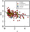 |
Fig. A.1. qIR as a function of redshift for all the 500 targets (grey points), the 4 VLBA-detected AGN (dark blue stars) and the 277 non-detections that constitute the M★-matched sample (red points). The green dots are the 42 non-detections which make the (M★, rms)-matched control sample. The black line is the NLS fit of all the targets described by the power law (1 + z)−0.13. |
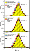 |
Fig. A.2. Normalized qIR distributions re-scaled to z0 = 0.5 (qIR, z0) for the control sample of VLBA non-detections (yellow histogram), while the 4 detections (light blue histogram) are shown both before (bottom panel) and after the VLBA AGN correction (top panel). The red Gaussian is the fit of the yellow+blue (or yellow) histograms, while the black curve is the Gaussian fit to the bootstrapped mirror distribution. |
Then, we compute the corrected qIR, z0 (qIR, z0, corr) of the 4 detections by subtracting the VLBA fluxes arising from the AGN, which is log(L1.4GHz, VLA − L1.4GHz, VLBA). Figure A.2 shows the distribution of the qIR, z0, corr of the 4 detections (blue histogram) and the qIR, z0 of the control sample (yellow histogram). The bin size is 0.2 dex, that is about twice larger than the average qIR uncertainty.
The red curve is the Gaussian fit of the real distribution. The gray curve is obtained by extracting 1000 values from the so-called “mirror distribution” (hatched histogram) using a bootstrap method, which would represent the distribution observed if all galaxies were star-forming. The errors used in the bootstrap are the 16th/84th percentiles of the 1000 values. The mirror distribution is obtained by unfolding the right-hand side of the distribution (above the peak, which is assumed to originate from pure SF) on the left side. A K-S test was not able to exclude that the mirror and the real distribution are drawn from different parent samples (with a p-value of 0.99). Accordingly, the median value of the real distribution, which is μR = 2.67  , and the median of the bootstrapped-mirror distribution (
 = 2.69
  ), are consistent between the errors on the medians, computed as the 16th/84th percentiles of the respective distributions divided by the root squared number of the total counts. Thus, as expected, the real distribution matches the mirrored one after subtracting the AGN contribution from the qIR, z0.
To explore the effects of the correction from the AGN contribution, we study qIR, z0 in two different scenarios: (1) without the VLBA correction for both detections and non-detections; and (2) only for the control sample of non-detections. Interestingly, the real and mirrored distributions are still statistically indistinguishable in the (1) case. The bottom panel of Fig. A.2, indeed, shows that μR = 2.65  and
and  = 2.68
  , which are (again) consistent within the error bars between each other and with the values in Fig. A.2. However, the difference between μR and μM is ∼ 0.03 dex and larger than when considering the AGN-corrected qIR, z0. We also observe a slight shift on the left side between the red and black curves, reflecting the fact that all the detections have qIR, z0 < μR. The shift, indeed, disappears in the central panel of Fig. A.2 when we consider SFG-only from the control sample. Finally, the values of μR are identical among the (1) and (2) cases. In conclusion, we can robustly claim that VLBA AGN contamination, despite being non-negligible for individual detections, does not impact at all the peak position (and the overall shape) of the original qIR distribution.
All Tables
All Figures
|
Fig. 1. RGB images of targets VLBA ID ‘338’ (top left), ‘351’ (top right), ‘408’ (bottom left), and ‘498’ (bottom right). These were obtained by combining the F150W, F277W, and F444W JWST/NIRCam filters (Franco et al. 2025) covering a 5″ × 5″ field of view. The NIRCam pixel scale is 30 mas. The white contours are the VLA 3 GHz levels (Smolčić et al. 2017) at three, four, five, and six times the rms (2.3 μJy/beam; the VLA beam size is 0.75″ as shown by the white circle in the bottom left). In the zoomed-in images of the red panels, the purple contours are the levels at two, three, four, five, and six times the image rms detected by the VLBA, which come from a 0.2″ × 0.2″ field of view (also outlined by the red square at the centers of the galaxies). The dotted purple contour also shows the −3 rms level. The VLBA beam size for each detection is: 26 × 5 mas2 (‘338’), 26 × 5 mas2 (‘351’), 28 × 5 mas2 (‘408’), and 23 × 6 mas2 (‘498’), with a similar position angle PA ∼ 162°. |
| In the text | |
|
Fig. 2. qIR distribution as function of host galaxy stellar mass for all 500 targets (gray points), four VLBA-detected AGNs (blue stars), and 277 non-detections part of the M★-matched sample (light blue points). The qIR of the detections account for the AGN emission detected by the VLBA (e.g., qIR, corr). The darker blue points are the 42 non-detections observed at sensitivities equal to or lower than the sensitivity of the detections, thus constituting the (M*, rms)- matched CS. The black line is the qIR versus log M★/M⊙ relation from Delvecchio et al. (2021) at ⟨z⟩∼1, and the shaded areas span the scatter of the IRRC at M★ > 1010.5 M⊙ from Delvecchio et al. (2021), of around ±0.22 dex and ±0.44 dex. |
| In the text | |
|
Fig. 3. Normalized distributions of difference between the observed qIR and the one expected from Eq. (4) (Delvecchio et al. 2021) based on the stellar mass and the redshift of the host galaxy, qIR (M★, z). The light purple histogram represents the distribution of the (M★, z)-CS. The stacked dark purple histogram (i.e., dark purple histogram on top of the light purple one) represents the detections, and the hatched orange histogram is the so-called mirror distribution, interpreted as the intrinsic qIR distribution of SFGs. The bootstrapped median values of the mirror distribution were fit with a Gaussian (red curve; see Sect. 5 for further details). Left panel: qIR was computed using the VLA luminosity coming from both star formation and AGN activity. Right panel: qIR, corr is measured after subtracting the AGN radio luminosity detected by the VLBA from the total radio VLA emission. |
| In the text | |
|
Fig. 4. Euclidean normalized radio-source number counts obtained by fitting with the Markov chain Monte Carlo algorithm, and the total radio luminosity function (LF) from Novak et al. (2018) using different evolving analytical LFs for AGN hosts (red line) and SF galaxies (blue line). The shaded areas encompass the 3σ errors from the χ2 fits performed on individual populations (for further details, see Novak et al. 2018). Gray circles are the number counts from Galluzzi et al. (2025) obtained from a compilation of radio observations with different instruments (e.g., VLA 1−3 GHz, ATCA, GMRT, LOFAR, MeerKAT, etc.), without any distinction between AGNs or SF. Red and black circles show the number counts from the VLBA CANDELS GOODS-North Survey (Deane et al. 2024) and VLBA 1.4 GHz COSMOS (Herrera-Ruiz et al. 2018) in the case of radio emission from AGN activity. The red star is the number count of the detections from the AGN-sCAN survey presented in this work. The gray arrow points toward the regime below our sensitivity limit, from which the number counts extrapolated from the red curve of Novak et al. (2018) of the 42 brightest AGN were extracted, in order to constrain upper limits on our results (see text in Sect. 7.1 for further details). |
| In the text | |
|
Fig. A.1. qIR as a function of redshift for all the 500 targets (grey points), the 4 VLBA-detected AGN (dark blue stars) and the 277 non-detections that constitute the M★-matched sample (red points). The green dots are the 42 non-detections which make the (M★, rms)-matched control sample. The black line is the NLS fit of all the targets described by the power law (1 + z)−0.13. |
| In the text | |
|
Fig. A.2. Normalized qIR distributions re-scaled to z0 = 0.5 (qIR, z0) for the control sample of VLBA non-detections (yellow histogram), while the 4 detections (light blue histogram) are shown both before (bottom panel) and after the VLBA AGN correction (top panel). The red Gaussian is the fit of the yellow+blue (or yellow) histograms, while the black curve is the Gaussian fit to the bootstrapped mirror distribution. |
| In the text | |
Current usage metrics show cumulative count of Article Views (full-text article views including HTML views, PDF and ePub downloads, according to the available data) and Abstracts Views on Vision4Press platform.
Data correspond to usage on the plateform after 2015. The current usage metrics is available 48-96 hours after online publication and is updated daily on week days.
Initial download of the metrics may take a while.