| Issue |
A&A
Volume 706, February 2026
|
|
|---|---|---|
| Article Number | A281 | |
| Number of page(s) | 15 | |
| Section | Planets, planetary systems, and small bodies | |
| DOI | https://doi.org/10.1051/0004-6361/202556358 | |
| Published online | 17 February 2026 | |
Where does the simplified stellar contamination model fail in exoplanet transmission spectroscopy?
1
Jet Propulsion Laboratory, California Institute of Technology, Pasadena,
California,
USA
2
Center for Radio Astronomy and Astrophysics Mackenzie (CRAAM), Mackenzie Presbyterian University,
Rua da Consolacão, 930, São Paulo,
São Paulo
01302-907,
Brazil
★ Corresponding author: This email address is being protected from spambots. You need JavaScript enabled to view it.
Received:
10
July
2025
Accepted:
5
January
2026
Abstract
Stellar photospheric heterogeneities (e.g., starspots and faculae) distort the apparent stellar spectrum during a transit and imprint wavelength-dependent biases on the measured planet–to–star radius ratio. This transit light source effect (TLSE) must be accounted for to obtain reliable atmospheric properties. A widely used approach is the Rackham–TLSE (R–TLSE) prescription, which applies a disk-averaged contamination correction based solely on the filling factor and spectral contrast. However, accurate transmission-spectroscopy interpretations require models that also account for limb darkening, the spatial distribution of active regions, and transit geometry. In this work, we incorporated these effects into a self-consistent, pixel-resolved framework, ECLIPSE-Xλ, and performed idealized, noise-free model–model comparisons against the R–TLSE approximation. Using three archetypal systems – the super-Earth LHS 1140 b, the mini-Neptune K2-18 b, and the hot Jupiter WASP-69 b – we show that disk-averaged TLSE corrections can differ from the self-consistent model by up to ~400 ppm in the optical for active hosts and non-equatorial transits, while remaining below ~10 ppm at near-infrared wavelengths where limb darkening is weaker. We then applied both approaches to the JWST/NIRISS SOSS transmission spectrum of LHS 1140 b. When limb darkening is artificially set to zero, ECLIPSE-Xλ recovers stellar-contamination parameters that closely match the reference R–TLSE solution, confirming that the two frameworks are consistent in the disk-averaged limit. With wavelength-dependent limb darkening included, however, reproducing the observed short-wavelength slope through stellar contamination alone requires very hot faculae (ΔTfac ≃ 600 K) covering ffac ≃ 0.35 of the visible hemisphere, corresponding to an equivalent circular facular region with radius ≃0.6 R⋆ (i.e., about 60% of the stellar radius) on the stellar disk. Such an extended, unocculted active region would be physically unlikely even for an active M dwarf. In this context, a purely stellar-contamination explanation for any residual optical slope would demand rather extreme facular populations; scenarios in which a genuine atmospheric contribution helps complement a more modest facular signal appear more physically plausible. Taken together, these results delineate the regime of validity of the R–TLSE approximation and underscore the need for geometry-aware stellar-heterogeneity models that explicitly account for limb darkening in high-precision transmission spectroscopy.
Key words: planets and satellites: atmospheres / planet-star interactions / stars: activity
© The Authors 2026
 Open Access article, published by EDP Sciences, under the terms of the Creative Commons Attribution License (https://creativecommons.org/licenses/by/4.0), which permits unrestricted use, distribution, and reproduction in any medium, provided the original work is properly cited.
This article is published in open access under the Subscribe to Open model. This email address is being protected from spambots. You need JavaScript enabled to view it. to support open access publication.
1 Introduction
Transmission spectroscopy has become a cornerstone technique for probing exoplanetary atmospheres, enabling the detection of chemical species, clouds, and scattering phenomena (Seager & Sasselov 2000; Brown et al. 2001; Charbonneau et al. 2002). However, the interpretation of these observations can be made more challenging by the presence of unocculted stellar photospheric heterogeneities (i.e., starspots and faculae), which distort the host star’s spectrum during transits and can mimic, or obscure, planetary atmospheric features (McCullough et al. 2014; Herrero et al. 2016; Rackham et al. 2017, 2018, 2019; Chachan et al. 2019; Iyer & Line 2020).
This source of systematic distortion, sometimes termed the transit light source effect (TLSE; Rackham et al. 2018), can produce apparent spectral modulation that surpasses the amplitude of genuine planetary atmospheric signals, particularly in systems with active M dwarfs and K-type stars. Although the James Webb Space Telescope (JWST) has unprecedented sensitivity to molecules such as CH4, CO2, and H2O, wavelength-dependent flux deficits introduced by unocculted spots and faculae can mimic molecular absorption bands, mask genuine spectral features, and bias the retrieved planet-to-star radius ratio, thereby complicating the interpretation of transmission spectra.
Rackham et al. (2018) introduced an analytic formalism – hereafter referred to as the Rackham-TLSE (R-TLSE) – which has since become the default means of mitigating stellar heterogeneity in atmospheric retrievals (e.g., Lim et al. 2023; May et al. 2023; Moran et al. 2023; Cadieux et al. 2024; Fournier-Tondreau et al. 2024; Petit dit de la Roche et al. 2024; Radica et al. 2025; Saba et al. 2025; Perdelwitz et al. 2025). Although the R-TLSE formalism has become a widely used approximation to model stellar contamination, it remains a simplified treatment of the effects of photospheric inhomogeneity. This approach describes the observed transit depth as a function of the contrast between the spectrum of the pristine photosphere (Fλ,phot), the spectrum of heterogeneity (Fλ,het), and the fractional coverage of the stellar disk by active regions (the filling factor). However, it does not account for the geometry of the transit chord, the stellar limb-darkening profile, or the spatial distribution of active regions across the stellar disk. As a result, atmospheric retrievals based solely on the TLSE formalism may be biased, particularly for systems with complex stellar activity that are observed with high-precision measurements.
In this paper, we present a comparative analysis of the R-TLSE approximation and our self-consistent modeling framework, ECLIPSE-Xλ. Using three representative exoplanetary systems – LHS 1140 b (a super-Earth), K2-18 b (a mini-Neptune), and WASP-69 b (a hot Jupiter) – we systematically quantified the extent to which these approximations influence spectral interpretations. Our findings clearly identify the conditions under which the R-TLSE approximation becomes unreliable, emphasizing the necessity for rigorous modeling of stellar activity to robustly disentangle planetary atmospheric signals from stellar contamination. Conversely, we also delineated the conditions under which the R-TLSE approximation remains valid, clarifying its domain of applicability.
The structure of this paper is as follows. In Sect. 2, we describe in detail the implementation of the ECLIPSE-Xλ model and the treatment of the R–TLSE prescription. In Sect. 3, we present an idealized, noise-free comparison that employs a differential error metric to quantify discrepancies between the two formalisms for the three aforementioned archetypal systems. We then apply both frameworks to the JWST Near-Infrared Imager and Slitless Spectrograph (NIRISS) Single-Object Slitless Spectroscopy (SOSS) observations of LHS 1140 b to assess their performance in a realistic observational context. We also discuss the implications of these findings for exoplanet atmosphere characterization, focusing on the regimes in which the R-TLSE correction loses validity while noting the specific conditions where it remains a useful simplification. The main conclusions are summarized in Sect. 4. Supplementary figures and retrieval outputs for K2-18 b and WASP-69 b are provided in Appendix A.
2 Methods
2.1 The ECLIPSE-Xλ starspot model
The ECLIPSE-Xλ1 (Sumida & Valio 2024, v1.0.0, Zenodo, doi:10.5281/zenodo.10888850, as developed on GitHub) is an advanced transit modeling tool built upon the foundation of the ECLIPSE2 model, originally proposed by Silva (2003). The code expanded the functionality of ECLIPSE, enabling it to simulate transit light curves across a wide range of wavelengths. The original ECLIPSE code was primarily designed to model active-region occultations using a 2D image of a synthetic star with spots on the surface of the limb-darkened stellar disk. By analyzing the photometric variations in the observed light curves during exoplanet transits, the physical properties of these systems can be inferred (e.g., Silva-Valio et al. 2010; Valio et al. 2017; Zaleski et al. 2019, 2020; Zaleski et al. 2022; Netto & Valio 2020; Araújo & Valio 2021; Valio & Araújo 2022; Valio et al. 2024).
To produce synthetic light curves, ECLIPSE-Xλ requires a 3D matrix to store stellar disk data at given wavelengths. This matrix encapsulates the spatial information of the star’s surface, enabling the code to simulate the effect of the transit and accurately compute the resulting flux variations. ECLIPSE-Xλ generates multiwavelength synthetic light curves that closely resemble the observed data and enables the calculation of the transit depth, which in turn enables the analysis of the atmospheric properties of the exoplanetary system under investigation. The code is primarily written in Python, although functions in C were implemented to enhance computational efficiency. Next, we detail the relevant input parameters of ECLIPSE-Xλ. Additional input parameters and their details can be found in Silva (2003).
Each starspot or facula is modeled as a circular disk and foreshortening of the spots and faculae is taken into account when they are close to the stellar limb. The spot size parameter is measured as a fraction of the stellar radius (Rs), and its position, namely latitude and longitude, is given with respect to the center of the stellar disk. The relative area of the stellar disk covered by starspots is the filling factor (hereafter ff), defined as
![Mathematical equation: $\[f f=\frac{A_{\mathrm{spot} / \mathrm{fac}}}{A_{\mathrm{s}}}=\left(\frac{R_{\mathrm{spot} / \mathrm{fac}}}{R_{\mathrm{s}}}\right)^2,\]$](/articles/aa/full_html/2026/02/aa56358-25/aa56358-25-eq1.png) (1)
(1)
where As and Rs are the area and radius of the stellar disk, and Aspot/fac and Rspot/fac are area and radius of the starspot or facula, respectively.
2.2 Constructing wavelength-dependent contrasts
In both the ECLIPSE-Xλ and R-TLSE (see Sect. 2.3) frameworks, stellar contamination can be expressed in terms of the wavelength-dependent contrast between the heterogeneous region and the pristine photosphere,
![Mathematical equation: $\[r_\lambda \equiv \frac{F_{\lambda, \mathrm{het}}}{F_{\lambda, \mathrm{phot}}},\]$](/articles/aa/full_html/2026/02/aa56358-25/aa56358-25-eq2.png) (2)
(2)
where Fλ,het and Fλ,phot are the disk-integrated fluxes from the heterogeneous region and the immaculate photosphere, respectively. When rλ is computed directly from high-resolution stellar-atmosphere spectra, for instance by interpolating PHOENIX specific intensities (Hauschildt et al. 1997; Hauschildt & Baron 1999; Husser et al. 2013) with LDTK (Parviainen & Aigrain 2015), it exhibits sharp, rapidly varying structure associated with atomic and molecular lines. Within a pixelated transit model that already includes wavelength-dependent limb darkening, feeding these line-dominated contrasts directly into the calculation leads to a strong and largely artificial amplification of individual spectral lines: the effective limb-darkening coefficients track these narrow features (see Fig. A.1) and imprint them onto the transit depth in a way that is not present in the original 1D atmosphere models.
To prevent this line-amplification problem, in this work we decoupled the smooth continuum behavior of the stellar intensity from the detailed line structure. For the computation of limb-darkening coefficients, we did not use monochromatic PHOENIX intensities, as this would propagate line structure directly into the limb-darkening law. Instead, we adopted a plane-parallel gray-atmosphere approximation in radiative equilibrium to obtain a spectrally smooth center-to-limb intensity profile. For each wavelength bin, we computed the emergent intensity Iλ(μ) as a function of μ = cos θ, normalized it by Iλ(1), and fit the four-parameter limb-darkening law of Claret (2000). The best-fitting coefficients are obtained by minimizing the squared residuals between the gray-atmosphere intensity profile and the parametric law using a Levenberg–Marquardt non-linear least-squares algorithm, following the same optimization strategy adopted by Claret et al. (2025) for PHOENIX-based JWST passbands. This yields a set of limb-darkening coefficients that varies smoothly with wavelength and is free from narrow spectral-line signatures. The same gray-atmosphere limb-darkening law is used for both the immaculate photosphere and the active regions, while their relative brightness is set by the black-body contrast:
![Mathematical equation: $\[\frac{I_{\mathrm{spot} / \mathrm{fac}}}{I_{\mathrm{star}}}=\frac{\exp~ [h c /(\lambda K_{\mathrm{B}} T_{\mathrm{star}})]-1}{\exp~ [h c /(\lambda K_{\mathrm{B}} T_{\mathrm{spot} / \mathrm{fac}})]-1},\]$](/articles/aa/full_html/2026/02/aa56358-25/aa56358-25-eq3.png) (3)
(3)
where h is the Planck constant, KB is the Boltzmann constant, Tstar is the stellar effective temperature, and Tspot/fac is the temperature of the starspot or facula.
At the same time, we sought to preserve the physical fidelity of the spectral-line pattern. To accomplish this, we decomposed the contrast into a smoothly varying continuum component and a high-frequency residual. This separation is most conveniently performed in logarithmic space,
![Mathematical equation: $\[\log~ r_\lambda=\log~ r_{\lambda, \mathrm{LP}}+\left[\log~ r_\lambda-\log~ r_{\lambda, \mathrm{LP}}\right],\]$](/articles/aa/full_html/2026/02/aa56358-25/aa56358-25-eq4.png) (4)
(4)
where log rλ,LP denotes a low-pass filtered version of the contrast (i.e., the smooth envelope or continuum), and the bracketed term contains the high-frequency residual Δ log rλ = log rλ − log rλ,LP, which encodes only the contribution from spectral lines. In practice, we computed rλ from PHOENIX stellar spectra for the photosphere and for the active regions applied a low-pass filter in wavelength to obtain log rλ,LP, and identify the residual Δ log rλ as the purely line-induced component.
For the self-consistent ECLIPSE-Xλ simulations, the smooth component rλ,LP is then replaced by the black-body contrast implied by Eq. (3), combined with the aforementioned gray-atmosphere limb-darkening description, while the residual Δ log rλ is applied as a multiplicative, wavelength-dependent correction at the level of the disk-integrated fluxes. In this way, the contaminated signal predicted by ECLIPSE-Xλ is governed by a spectrally smooth continuum and physically motivated limb darkening, while the fine spectral structure of realistic stellar spectra is still consistently incorporated into the model.
2.3 R-TLSE model comparison
According to Rackham et al. (2018), the parameter ϵλ,het represents the correction factor introduced by the TLSE. It quantifies the discrepancy between the observed transit depth and the intrinsic transit depth expected in the absence of stellar heterogeneities at a given wavelength λ. The factor ϵλ is defined as the ratio of the observed transit depth to the intrinsic transit depth, accounting for the presence of unocculted stellar spots and faculae. Mathematically, it is expressed as
![Mathematical equation: $\[\epsilon_{\lambda, \text {het }}=\frac{1}{1-f_{\text {het}\left(1-\frac{F_{\lambda, \text {het}}}{F_{\lambda, \text {phot}}}\right)}}.\]$](/articles/aa/full_html/2026/02/aa56358-25/aa56358-25-eq5.png) (5)
(5)
If ϵλ > 1, the measured transit depth is overestimated, indicating an excess of dimmer regions on the stellar surface (e.g., unocculted starspots). Conversely, if ϵλ < 1, the transit depth is underestimated, suggesting an excess of brighter regions, such as faculae.
In this study we compared the simple R-TLSE model proposed by Rackham et al. (2019) to our TLSE model, which incorporates additional physical effects. The comparison was carried out in a straightforward and systematic manner. First, we simulated two scenarios: a pristine, unspotted star (serving as a baseline) and a star with heterogeneous surface features (incorporating stellar contamination). For the TLSE, we used the unspotted star as a reference and inferred the stellar contamination through the contamination factor ϵλ,het, allowing for a direct evaluation against the theoretical predictions of the R-TLSE model. To quantify discrepancies between the frameworks, we introduced the error
![Mathematical equation: $\[\text { Error }=D_{\lambda, \text { ECLIPSE}}-D_{\lambda, \text {R-TLSE}},\]$](/articles/aa/full_html/2026/02/aa56358-25/aa56358-25-eq6.png) (6)
(6)
where Dλ,ECLIPSE is the transit depth obtained from our simulations, and Dλ,R-TLSE is the transit depth computed using Eq. (5) of R-TLSE (Rackham et al. 2018). This metric isolates systematic biases introduced by the R-TLSE’s simplified treatment of limb darkening and transit geometry. Positive error values indicate that R-TLSE predicts a shallower transit than ECLIPSE-Xλ (i.e., it overcorrects for stellar contamination), whereas negative values indicate that R-TLSE predicts a deeper transit and thus under-corrects for stellar contamination.
To guide the interpretation of the forthcoming detailed comparison in Sect. 3, Table 1 provides a concise overview of the conceptual differences between the R–TLSE and ECLIPSE-Xλ frameworks, particularly regarding limb darkening, transit geometry, and the treatment of stellar surface heterogeneities.
3 Results and discussion
This section combines an idealized, purely model–model comparison (Sect. 3.1) with an application to observational data (Sect. 3.2). In Sect. 3.1 (Cases 1–3), we compute noise-free transmission spectra with ECLIPSE-Xλ and with the R-TLSE approximation using the same black-body description for the photosphere and active regions, without including PHOENIX stellar-atmosphere spectra or any instrument response. This common black-body prescription avoids mixing a 1D PHOENIX atmosphere with the pixelized stellar disk in ECLIPSE-Xλ and ensures that the discrepancies we report are driven solely by the treatment of stellar heterogeneity and transit geometry, rather than by differences in radiative-transfer inputs or spectral binning. When we applied both approaches to the JWST/NIRISS SOSS observations of LHS 1140 b (Sect. 3.2), we instead adopted PHOENIX model atmospheres for both the photosphere and the active regions and fold the models through the NIRISS throughput and spectral resolution, so that the comparison reflects a realistic observational context and the impact of these systematic differences can be assessed relative to the actual measurement uncertainties.
3.1 Idealized model–model comparison
To assess how our model deviates from the R-TLSE in its predictions, we performed simulations under the following scenarios:
Case 1 – fixed filling factor, variable temperature contrast: the filling factor was set to 0.15 for both starspots and faculae, while the temperature contrast ΔT was varied from −300 K to +300 K. This disentangles spectral biases driven purely by temperature differences. The adopted upper limit for the filling factor (fhet = 0.15) is motivated by recent atmospheric retrievals based on JWST transmission spectra, which inferred comparable starspot and faculae coverages in M-dwarf systems. Specifically, May et al. (2023) and Cadieux et al. (2024) reported coverages of up to 40% for GJ 1132 b and 30% for LHS 1140 b, based on NIRSpec and NIRISS data, respectively.
Case 2 – fixed temperature contrast, variable filling factor: a constant temperature contrast of |ΔT| = 300 K was applied, while the filling factor was varied from 0.01 to 0.15. This isolates the effect of the spatial coverage of active regions. We constrained the temperature contrast between active regions and the photosphere to ±300 K, consistent with values inferred from those retrievals (May et al. 2023; Cadieux et al. 2024) and from solar analog studies (e.g., Meunier et al. 2010).
Case 3 – variable position of active regions: We fixed both the temperature contrast and filling factor, but systematically varied the projected position of starspots and faculae on the stellar disk by changing their latitude and longitude. This evaluates the geometric dependence of stellar contamination and its impact on spectral bias.
The results for Cases 1 and 2, for the planet LHS 1140 b, are presented in Figs. 1 and 2, respectively. Parallel analyses for K2-18 b and WASP-69 b are provided in Fig. A.2.
The pattern observed in the curves in Figs. 1 and 2 – and Fig. A.2 – aligns with expectations: the largest wavelength-dependent errors between the R-TLSE approximation and the ECLIPSE-Xλ model occur at wavelengths where limb darkening induces the most pronounced brightness gradients across the stellar disk, particularly in the optical regime (see Alexoudi et al. 2020). For LHS 1140 b, our simulations reveal significant discrepancies, especially at optical wavelengths. At wavelengths shorter than 800 nm, systematic biases exceed 50 ppm, reaching maxima of approximately 170 ppm for unocculted starspots and 140 ppm for faculae near 500 nm.
These offsets arise from the R-TLSE’s neglect of wavelength-dependent limb-darkening contrasts and the geometric modulation of stellar contamination. At longer wavelengths (1000–2000 nm), the error diminishes to below 10 ppm, as limb-darkening effects weaken and stellar spectral energy distributions become smoother. Adopting the system parameters of Cadieux et al. (2024), a single atmospheric scale height of an N2-dominated atmosphere on LHS 1140 b corresponds to only a few ppm (on the order of 4–5 ppm) in transit depth; the 50–170 ppm optical discrepancies between ECLIPSE-Xλ and the R-TLSE approximation therefore amount to on the order of 10–40 atmospheric scale heights. This wavelength-dependent bias, therefore, has direct implications for atmospheric retrievals and for the interpretation of slope-like features in terms of Rayleigh scattering or aerosols. Previous TLSE-based retrieval studies have already shown that specific stellar modeling assumptions and particular treatments of stellar contamination can imprint or distort such apparent slopes, biasing the inferred atmospheric properties (see, for example, Zhang et al. 2018; Iyer & Line 2020; Rackham & de Wit 2024).
In their study, Cadieux et al. (2024) report a marginal detection of N2 in the atmosphere of the temperate super-Earth LHS 1140 b at a significance level of 2.3σ. This result is primarily driven by a modest short-wavelength spectral slope (500–800 nm), which they interpret as Rayleigh scattering from a high-mean-molecular-weight (high-MMW) atmosphere dominated by N2. Although the observed transmission spectrum remains largely flat at infrared wavelengths (>1 μm), it exhibits a subtle blueward slope in the visible regime – precisely where the R-TLSE approximation has the greatest potential for errors. The same analysis also reveals a statistically significant detection (5.8 σ) of unocculted stellar faculae, covering approximately 20% of the stellar disk. This contamination is modeled using the R-TLSE formalism. However, despite the inclusion of this correction, the fit to the data exhibits a relatively high reduced chi-squared, hinting that the R-TLSE may not fully capture the spectral distortions induced by photospheric heterogeneities.
Given the significant discrepancies between the R-TLSE approximation and the ECLIPSE-Xλ model, interpretations of an N2-rich atmosphere based solely on this simplified treatment of the R-TLSE should be approached with caution. Notably, the spectral region supporting the N2 signal coincides with wavelengths where inaccuracies inherent in the R-TLSE are expected to peak – precisely where the observational data also show their largest uncertainties and dispersion. A more comprehensive examination of the fit and its limitations is presented in Sect. 3.2.
For the sub-Neptune K2-18 b (see Fig. A.2, first and second rows), our simulations show that in the optical range (500–600 nm), the R-TLSE approximation and our self-consistent model can differ by about 80–100 ppm. Such offsets are comparable to the amplitude of key atmospheric signals in sub-Neptune spectra. Beyond 1.5 μm, however, these discrepancies drop below 10 ppm, indicating that the R-TLSE remains reasonably accurate in the near-infrared (NIR), consistent with previous investigations that robustly detected methane (CH4) via R-TLSE-based equation (e.g., Madhusudhan et al. 2023; Schmidt et al. 2025). Schmidt et al. (2025) incorporated stellar contamination models (fhet = ![Mathematical equation: $\[5_{-2}^{+3}\]$](/articles/aa/full_html/2026/02/aa56358-25/aa56358-25-eq7.png) % at ΔT ≈ 500 ± 350 K cooler than the photosphere), showing that while these corrections minimally affect CH4 inferences, they are crucial to avoid false positives in trace species such as CO2.
% at ΔT ≈ 500 ± 350 K cooler than the photosphere), showing that while these corrections minimally affect CH4 inferences, they are crucial to avoid false positives in trace species such as CO2.
In contrast, Madhusudhan et al. (2023) found no detectable stellar activity in M dwarfs hosting Hycean candidates. However, the apparently quiescent behavior of M-type hosts such as K2-18 may be partly driven by orbital geometry: for transits probing mid-latitude chords (~40°), our ECLIPSE-Xλ simulations show that a spotless photosphere already yields nearly wavelength-independent transit depths, effectively removing most of the geometrical slope. In this “flat-geometry” regime, even modest chromatic stellar contamination or weak atmospheric gradients can produce shallow slopes that are comparable to the current observational uncertainties, making it difficult to distinguish genuinely high-MMW, cloud-dominated atmospheres from cases where residual stellar heterogeneity and geometry conspire to flatten the observed spectrum. This underscores the need for stellar-heterogeneity models that are explicitly consistent with the system’s orbital geometry. A more detailed discussion of the impact of limb darkening and transit geometry on transmission spectra is provided in Alexoudi et al. (2020) and in Sect. 3.2.
In the case of the hot Jupiter WASP-69 b (see Fig. A.2, third and fourth rows), the differences between the R-TLSE and the ECLIPSE-Xλ model are substantially greater than those observed for LHS 1140 b and K2-18 b. Around 500 nm, these discrepancies can reach up to ~400 ppm. Moreover, up to roughly 1500 nm, our simulations indicate that the errors remain above 50 ppm, eventually dropping to 50–10 ppm in the remainder of the spectrum.
Such large discrepancies become even more significant in light of recent VLT spectrophotometry of WASP-69 b obtained with the FOcal Reducer and low dispersion Spectrograph 2 (FORS2), covering 340–1100 nm (Petit dit de la Roche et al. 2024). Their retrievals, which applied the R-TLSE correction equation to account for stellar contamination, inferred an extensive facula coverage of ~30% with a temperature excess of ΔT ≈ 230 ± 70 K. For a K-type star, such a large facular filling factor is already somewhat extreme and is likely highly biased, given the simplified assumptions inherent to the correction method. Moreover, the planet’s mid-latitude impact parameter (b ≈ 0.66) implies that the transit chord probes intermediate stellar latitudes, close to the 40–45° regime where our ECLIPSE-Xλ simulations predict nearly wavelength-independent transit depths for a spotless photosphere. In this resulting “flat-geometry” configuration, most of the purely geometrical slope is removed, so the negative optical slope seen in the FORS2 transmission spectrum is expected to arise primarily from the combined effects of stellar heterogeneity and atmospheric gradients, rather than from geometry alone.
Additionally, a large facula filling factor naturally induces a negative spectral slope in the optical, as illustrated in Fig. 3 of Petit dit de la Roche et al. (2024). In our self-consistent ECLIPSE-Xλ calculations, the disagreement with the R-TLSE-based predictions grows systematically with increasing facula coverage: for high filling factors, the R-TLSE prescription produces much stronger chromatic stellar contamination than the pixel-resolved model. This behavior suggests that, when applied in the mid-latitude geometric regime of WASP-69 b, the R-TLSE approach can substantially overpredict the level of stellar contamination and thus overestimate the facula filling factor.
Prior atmospheric analyses based on Hubble Space Telescope observations obtained with the Space Telescope Imaging Spectrograph (STIS) and the Wide Field Camera 3 (WFC3) suggested strong Rayleigh scattering slopes, which were interpreted as evidence of high-altitude aerosols (e.g., Estrela et al. 2021). However, the steep slope reported in that study might instead result from unocculted starspots or faculae, since our contamination-free simulations yield a flat spectral baseline for WASP-69 b. Therefore, it remains uncertain whether these optical slopes arise from genuine atmospheric properties or are artifacts of stellar heterogeneity.
Meanwhile, Murgas et al. (2020) reported an even steeper optical slope with Gran Telescopio Canarias (GTC) observations obtained with the Optical System for Imaging and low-Intermediate-Resolution Integrated Spectroscopy (OSIRIS), consistent with Rayleigh scattering, which they modeled with fspot = 0.55 and ffac = 0.15 (ΔTspot = −122 K, ΔTfac = +72 K). Such extreme filling factors almost certainly do not trace stellar heterogeneity alone, but rather reflect a degeneracy in which part of the atmospheric signal is absorbed into the stellar-contamination term by the R-TLSE formalism. For instance, a spot filling factor of fspot = 0.55 corresponds to an equivalent circular heterogeneous region with radius Rhet ≃ 0.75 R⋆; when the facular contribution is included, the total coverage (fhet = fspot + ffac ≃ 0.70) implies Rhet ≃ 0.83 R⋆. In our 2D stellar model, such a vast coherent active region on the visible hemisphere would be difficult to reconcile with the mid-latitude transit chord of WASP-69 b without the planet occulting a substantial fraction of these inhomogeneities. This strongly suggests that the steep OSIRIS slope is more naturally explained by a combination of genuine atmospheric opacity and more moderate stellar heterogeneity than by the extreme active-region coverages implied by the disk-averaged R-TLSE prescription.
Importantly, recent JWST eclipse observations of WASP-69 b also support the presence of high-altitude aerosols on the dayside hemisphere (Schlawin et al. 2024). Although those emission spectra are unaffected by stellar heterogeneity, the fact that cloud-free models fail to reproduce the observed flux reinforces the interpretation that aerosols, rather than stellar contamination, likely shape the NIR features. This highlights the need for transmission analyses to account for both stellar and planetary contributions explicitly, as done in ECLIPSE-Xλ, which treats stellar contamination independently of atmospheric retrievals but allows for their disentanglement across wavelengths.
Despite the fact that our simulations isolate stellar activity signals by fixing the temperature contrast or filling factor while varying the other, we further explored a scenario that systematically spans the full parameter space between these variables. This approach quantifies how degeneracies between temperature and spatial coverage influence model divergences. The results, illustrated in Fig. 3 for all three exoplanets, reveal wavelength-dependent discrepancies between our method and the R-TLSE correction equation. For this analysis, we focused on 600 nm, a wavelength selected to align with the lower limit of the JWST/NIRSpec observational range. According to this figure, we can clearly identify where the discrepancies are minimal (pink hues) and where they become more pronounced (blue). As expected, our model and the R-TLSE approximation tend to agree when the temperature of the star’s active regions is closer to its effective temperature. Conversely, the error increases toward the upper portion of the diagram, where filling factors are largest and the active regions exhibit the greatest temperature contrast relative to the stellar photosphere.
It is worth emphasizing that, in our simulations, the active region was placed as centrally as possible on the stellar disk without being occulted. In other words, the peak localized brightness at the disk center was effectively suppressed by stellar activity. Nevertheless, our model also includes additional positional parameters that further complicate both the analysis and the potential mitigation of stellar contamination in transmission spectra. These include the number of starspots and faculae, and their spatial location (closer to the center or to the limb of the stellar disk). Each of these parameters can be varied independently, producing a vast array of combinations and potentially leading to significant computational demands when fitting to observational data. To illustrate this complexity, we focused exclusively on the exoplanet LHS 1140 b, varying the location of the active regions.
In Fig. 4, which corresponds to Case 3, we show the impact of the active region’s position on the stellar disk by systematically varying its location. To this end, we considered only the simulations with temperature variations, which are represented by the colors of faculae and starspots. We started with the active region at 15° latitude and 0° longitude, gradually shifting to 35° latitude and 35° longitude, effectively moving it from the center toward the stellar limb. At each step, we observe substantial discrepancies between our model and R-TLSE. Initially, the result is the same as in Fig. 1, since the active region is placed exactly as in the previously discussed scenario. However, in the right panel of the upper row, where the latitude is increased by just 10°, an intriguing effect emerges: the error associated with both starspots and faculae undergoes a sign reversal beyond the optical regime. As a result, in the NIR range, the R-TLSE approximation – previously overestimating these contributions – now underestimates the impact of stellar heterogeneities.
In the lower panels of Fig. 4, we push our analysis to more extreme geometries by placing active regions closer to the stellar limb. In the left panel, the active region is positioned at a latitude of 25° and a longitude of 15°, shifting the sign-inversion boundary toward shorter wavelengths and thereby substantially reducing the errors in the optical range (where the largest discrepancies were previously observed). In the right panel of the second row, we consider an even more extreme configuration, with the active region located near both high latitudes and high longitudes – practically on the stellar limb. Here, the sign inversion becomes fully established, the errors again escalate due to the pronounced influence of limb darkening and foreshortening. As the spot or facula moves to the limb, its projected area – and thus its impact on the stellar flux – becomes disproportionately large, significantly exacerbating the shortcomings of the R-TLSE-based equation.
Overall, these analyses, depicted in the panels of Fig. 4, underscore that inaccuracies associated with the R-TLSE correction equation grow significantly when active regions are located near the center or the stellar limb, due to the intricate interplay of limb darkening and stellar surface geometry. This highlights the necessity for self-consistent modeling of stellar contamination when interpreting transmission spectra, especially for exoplanets transiting active stars.
Qualitative comparison of the R-TLSE formalism and ECLIPSE-Xλ.
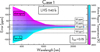 |
Fig. 1 Wavelength-dependent errors between ECLIPSE-Xλ and the R-TLSE (Eq. (6)) for LHS 1140 b, computed using a fixed filling factor (fhet = 0.15) and a temperature contrast (ΔT) varying from −300 K (spots) to +300 K (faculae). The largest discrepancies arise in the optical range (500–800 nm), where steep limb-darkening gradients drive optical biases. The dashed lines mark reference levels at −50, −20, −10, 10, 20, and 50 ppm, serving as a visual aid to highlight variations in the data. By construction, positive values of the error indicate that R-TLSE predicts a shallower transit depth than ECLIPSE-Xλ (overcorrecting stellar contamination), while negative values correspond to a deeper R-TLSE transit (under-correcting contamination). |
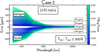 |
Fig. 2 Discrepancies, defined by Eq. (6), as a function of fixed temperature contrast (Tstar ± 300) and with the filling factor (fhet) varied from 0.01 to 0.15. Positive errors (R-TLSE overestimation) dominate for cool spots, while negative errors (R-TLSE underestimation) arise for hot faculae. Extreme cases (e.g., fhet = 0.15, ΔT = ±300 K) show maximal divergence. The dashed lines delineate boundaries at −50, −20, −10, 10, 20, and 50 ppm. |
 |
Fig. 3 2D parameter space exploration showing the discrepancies (Eq. (6)) at a representative wavelength of 600 nm. Each panel corresponds to a different exoplanetary system: LHS 1140 b (left panel), K2-18 b (middle panel), and WASP-69 b (right panel). Color scales indicate the difference between our model and the R-TLSE correction equation, as a function of filling factor and temperature contrast. |
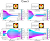 |
Fig. 4 Effect of the active region’s spatial position on the stellar disk for LHS 1140 b, illustrating the wavelength-dependent error between ECLIPSE-Xλ and R-TLSE. Each curve corresponds to a different temperature of the active region (spot or facula). The four panels examine positions gradually shifting from close to disk center (15° latitude, 0° longitude) toward the limb (35° latitude, 35° longitude). A sign inversion emerges at intermediate positions beyond the optical wavelengths (right panel, first row). The lower panels depict more extreme cases with active regions placed even closer to the limb, showing that the sign-inversion boundary moves to shorter wavelengths, significantly altering and reducing errors in the optical regime, while further limb positioning exacerbates R-TLSE inaccuracies due to enhanced limb darkening and foreshortening. Positive errors mean that R-TLSE predicts a shallower transit than ECLIPSE-Xλ (overcorrecting contamination), whereas negative errors mean that R-TLSE predicts a deeper transit (under-correcting contamination). |
3.2 Application to observational data: LHS 1140 b
The transmission spectrum analyzed in this section is the combined JWST/NIRISS SOSS dataset of LHS 1140 b, consisting of two transits reduced and binned to R ~ 100 (Cadieux et al. 2024)3 For reference, the R-TLSE column in Table 2 reproduces the TLS-only stellar-contamination solution reported by Cadieux et al. (2024) at this resolution. We then fit the same R ~ 100 spectrum with ECLIPSE-Xλ by exploring a regular grid in the temperatures and filling factors of spots and faculae. For each grid point, ECLIPSE-Xλ computes the corresponding disk-integrated photosphere + activity spectrum, folds it through the NIRISS/SOSS throughput and spectral response to match the R ~ 100 channel grid, incorporates the TLSE in the model transit depths, and evaluates the resulting transmission spectrum against the observations via a χ2 statistic. The best-fitting solutions for models with our nominal limb-darkening treatment and with limb darkening set to zero (limb-darkening coefficients, LDCs = 0) are shown in Fig. 5 and summarized in Table 2.
As a first step, we compared the ECLIPSE-Xλ retrieval with limb darkening switched off (LDCs = 0) to the reference R-TLSE solution. When all limb-darkening coefficients are set to zero, the stellar disk becomes uniformly bright and the transit chord no longer samples any center-to-limb intensity gradient. In this case, the pixelized ECLIPSE-Xλ simulations approach the same disk-averaged description of stellar contamination that underlies the R-TLSE formalism. This modeling configuration is closely related to the situation discussed by Alexoudi et al. (2020), who show that removing the host-star limb darkening causes the impact-parameter degeneracy to disappear: the inferred planet-to-star radius ratio Rp/Rs no longer exhibits any wavelength-dependent offset and remains constant across the spectrum. Adopting this limb-darkening-free configuration in ECLIPSE-Xλ therefore eliminates that particular source of bias and isolates any residual differences between our model and R-TLSE.
Table 2 shows that, under these conditions, the stellar-contamination parameters recovered by ECLIPSE-Xλ (LDCs = 0) remain very close to the R-TLSE solution. The inferred photospheric temperatures agree at the ~1σ level (Tphot = ![Mathematical equation: $\[3073_{-54}^{+45}\]$](/articles/aa/full_html/2026/02/aa56358-25/aa56358-25-eq24.png) K for R-TLSE vs.
K for R-TLSE vs. ![Mathematical equation: $\[3100_{-40}^{+40}\]$](/articles/aa/full_html/2026/02/aa56358-25/aa56358-25-eq25.png) K for ECLIPSE-Xλ with LDCs = 0), and the facular filling factors are essentially identical (ffac =
K for ECLIPSE-Xλ with LDCs = 0), and the facular filling factors are essentially identical (ffac = ![Mathematical equation: $\[0.21_{-0.12}^{+0.14}\]$](/articles/aa/full_html/2026/02/aa56358-25/aa56358-25-eq26.png) compared to
compared to ![Mathematical equation: $\[0.22_{-0.050}^{+0.052}\]$](/articles/aa/full_html/2026/02/aa56358-25/aa56358-25-eq27.png) ). A small but noticeable difference arises in the facular temperature, with ECLIPSE-Xλ(LDCs = 0) favoring hotter faculae (Tfac =
). A small but noticeable difference arises in the facular temperature, with ECLIPSE-Xλ(LDCs = 0) favoring hotter faculae (Tfac = ![Mathematical equation: $\[3370_{-62}^{+50}\]$](/articles/aa/full_html/2026/02/aa56358-25/aa56358-25-eq28.png) K) than the R-TLSE retrieval (
K) than the R-TLSE retrieval (![Mathematical equation: $\[3155_{-91}^{+69}\]$](/articles/aa/full_html/2026/02/aa56358-25/aa56358-25-eq29.png) K), while keeping ffac almost unchanged. A plausible interpretation is that this offset reflects geometric effects that are explicitly included in ECLIPSE-Xλ, even when limb darkening is switched off: the model still accounts for foreshortening and for the localized position of active regions on the stellar disk, whereas the R-TLSE approximation assumes a spatially uniform, disk-averaged coverage. In our pixel-based framework, part of the geometric dilution of facular brightness can therefore be absorbed into a slightly higher intrinsic facular temperature rather than into a different filling factor, leading to the modest temperature shift seen in Table 2, while preserving an almost identical overall level of stellar contamination.
K), while keeping ffac almost unchanged. A plausible interpretation is that this offset reflects geometric effects that are explicitly included in ECLIPSE-Xλ, even when limb darkening is switched off: the model still accounts for foreshortening and for the localized position of active regions on the stellar disk, whereas the R-TLSE approximation assumes a spatially uniform, disk-averaged coverage. In our pixel-based framework, part of the geometric dilution of facular brightness can therefore be absorbed into a slightly higher intrinsic facular temperature rather than into a different filling factor, leading to the modest temperature shift seen in Table 2, while preserving an almost identical overall level of stellar contamination.
When full limb darkening is included, the ECLIPSE-Xλ fit departs more markedly from the R-TLSE solution unless the model is allowed to explore rather extreme facular coverages. As summarized in Table 2, the R-TLSE analysis favors a relatively cool photosphere and modestly hotter faculae (Tphot = ![Mathematical equation: $\[3073_{-54}^{+45}\]$](/articles/aa/full_html/2026/02/aa56358-25/aa56358-25-eq30.png) K and Tfac =
K and Tfac = ![Mathematical equation: $\[3155_{-91}^{+69}\]$](/articles/aa/full_html/2026/02/aa56358-25/aa56358-25-eq31.png) K, with ffac =
K, with ffac = ![Mathematical equation: $\[0.21_{-0.12}^{+0.14}\]$](/articles/aa/full_html/2026/02/aa56358-25/aa56358-25-eq32.png) ). By contrast, in the fully limb-darkened ECLIPSE-Xλ simulations, where we allowed unocculted faculae to occupy up to ffac ≤ 0.40 of the visible hemisphere, the optimizer naturally drives the solution toward very hot and spatially extended faculae. the best-fitting self-consistent model for LHS 1140 b converges to a photospheric temperature very similar to the R-TLSE value (Tphot =
). By contrast, in the fully limb-darkened ECLIPSE-Xλ simulations, where we allowed unocculted faculae to occupy up to ffac ≤ 0.40 of the visible hemisphere, the optimizer naturally drives the solution toward very hot and spatially extended faculae. the best-fitting self-consistent model for LHS 1140 b converges to a photospheric temperature very similar to the R-TLSE value (Tphot = ![Mathematical equation: $\[3099_{-47}^{+44}\]$](/articles/aa/full_html/2026/02/aa56358-25/aa56358-25-eq33.png) K), but with much hotter faculae (Tfac =
K), but with much hotter faculae (Tfac = ![Mathematical equation: $\[3701_{-44}^{+54}\]$](/articles/aa/full_html/2026/02/aa56358-25/aa56358-25-eq34.png) K, ΔTfac ≈ 600 K) covering ffac =
K, ΔTfac ≈ 600 K) covering ffac = ![Mathematical equation: $\[0.35_{-0.06}^{+0.03}\]$](/articles/aa/full_html/2026/02/aa56358-25/aa56358-25-eq35.png) of the stellar disk. This configuration lies close to the geometric limit at which active regions would start intersecting the transit chord, and it yields a reduced χ2 for the limb-darkened fit that is comparable to the R-TLSE solution, at the expense of invoking a very large population of unocculted faculae.
of the stellar disk. This configuration lies close to the geometric limit at which active regions would start intersecting the transit chord, and it yields a reduced χ2 for the limb-darkened fit that is comparable to the R-TLSE solution, at the expense of invoking a very large population of unocculted faculae.
This behavior is readily understood once we account for the impact of limb darkening on the baseline transit geometry. Even in the absence of stellar heterogeneities, a limb-darkened star does not, in general, produce a perfectly flat transmission spectrum: for a nearly central transit, the combination of impact parameter and center-to-limb intensity variations naturally induces a modest positive slope in Rp/Rs at optical wavelengths, as highlighted by Alexoudi et al. (2020). In the R-TLSE (or LDCs = 0) limit, this geometric effect is explicitly removed by construction, because the stellar disk is assumed to be uniformly bright, and the baseline spectrum is flat in the absence of active regions. Unocculted faculae then act on top of this flat reference and directly imprint a net slope. In the fully limb-darkened ECLIPSE-Xλ framework, on the other hand, we already started from a positively sloped baseline set by the transit geometry; adding unocculted faculae must first compensate for this geometrically induced trend before it can reproduce any additional slope of opposite sign. The optimizer therefore tends to increase Tfac and to push ffac toward the upper bound of the prior in order to counteract the limb-darkening-driven slope. However, foreshortening and the localized nature of the active regions limit how much extra bias they can introduce into the disk-integrated flux. As a result, R-TLSE-like slopes can be reproduced in the fully limb-darkened simulations only in the extreme regime of very hot faculae covering ≳30–40% of the visible hemisphere. More moderate facular configurations naturally produce a shallower contamination signal, implying that any residual optical slope is likely to include a genuine atmospheric contribution, potentially combined with a less extreme level of stellar contamination, rather than being solely due to unocculted faculae.
Stellar-contamination retrieval summary for LHS 1140 b.
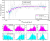 |
Fig. 5 Comparison between ECLIPSE-Xλ and the R-TLSE approximation for the JWST/NIRISS SOSS transmission spectrum of LHS 1140 b. Top: combined R ~ 100 NIRISS spectrum (gray points with error bars), together with the best-fitting stellar-contamination models. The magenta curve shows the self-consistent ECLIPSE-Xλ fit that includes wavelength-dependent limb darkening, the cyan curve shows the corresponding fit with limb darkening set to zero (LDCs = 0), and the black curve reproduces the TLS-only stellar-contamination model from the R-TLSE reference retrieval (see Cadieux et al. 2024). The small-scale structure along the model curves follows atomic and molecular absorption bands in the underlying PHOENIX spectra: TiO/VO and metal lines dominate in the optical, while broad features in the NIR are mainly shaped by H2O bands and CO absorption complexes longward of ~2.2 μm, i.e., precisely the wavelength ranges where exoplanet transmission spectra are usually interpreted in terms of H2O, CH4, and CO absorption. Bottom: 1D marginal distributions for the stellar-contamination parameters in the ECLIPSE-Xλ fits, for the cases with limb darkening (top row, magenta) and with LDCs= 0 (bottom row, cyan). From left to right, panels show the filling factor and temperature of spots (fspot, Tspot) and faculae (ffac, Tfac). Vertical lines indicate the median (solid) and 16th–84th percentile (dashed) intervals reported in Table 2. |
4 Summary and conclusions
This study demonstrates that the R-TLSE approximation introduces systematic, wavelength-dependent biases in exoplanet transmission spectra, especially at optical wavelengths where limb-darkening gradients and transit geometry play a dominant role. Through idealized, noise-free simulations (Sect. 3.1), we compared the disk-averaged R-TLSE correction to our self-consistent ECLIPSE-Xλ framework, which incorporates wavelength-dependent limb darkening, the spatial distribution of active regions, and the full transit geometry, and we quantified system-specific discrepancies for three archetypal planets. We then applied both approaches to the JWST/NIRISS SOSS observations of LHS 1140 b (Sect. 3.2), using the data as a testbed for assessing the practical impact of these differences on atmospheric interpretation. Overall, our analysis shows that the scale of the R-TLSE-induced errors must be assessed on a case-by-case basis.
For LHS 1140 b, a super-Earth orbiting an M dwarf, we find peak discrepancies of 170 ppm due to starspots and 140 ppm due to faculae at 500 nm, driven primarily by the R-TLSE’s neglect of optical limb-darkening contrasts. These errors decrease to below 10 ppm at NIR wavelengths above 1000 nm, where limb-darkening effects are weaker, rendering R-TLSE-based retrievals more reliable. However, in the optical regime (500–800 nm), R-TLSE inaccuracies become largest and may contribute to marginal atmospheric detections. Notably, the spectral region supporting the tentative N2 signal reported by Cadieux et al. (2024) coincides with wavelengths where R-TLSE inaccuracies are expected to peak and with the part of the spectrum that exhibits the largest observational uncertainties and dispersion, making any N2 detection claim especially sensitive to the adopted stellar-contamination model.
In the case of K2-18 b, a mini-Neptune also orbiting an M dwarf, the idealized simulations show that in the optical range (500-600 nm) the R-TLSE approximation and the self-consistent model can differ by about 80–100 ppm, which is comparable to the amplitude of key atmospheric features in sub-Neptune spectra. The planet’s mid-latitude transit geometry (b ≃ 0.65) places the system in a “flat-geometry” regime in which a spotless, limb-darkened star already yields nearly wavelength-independent transit depths. In this configuration, modest chromatic stellar contamination or weak atmospheric gradients can produce shallow slopes that are comparable to current observational uncertainties, making it difficult to distinguish genuinely high-mean-molecular-weight, cloud-dominated atmospheres from more extended envelopes combined with residual stellar heterogeneity. At NIR wavelengths (λ ≳ 1.5 μm), however, ECLIPSE-Xλ and R-TLSE agree to within ~10 ppm, consistent with previous analyses, showing that methane detections based on R-TLSE-corrected spectra are robust, while inferences for secondary species such as CO2 remain more vulnerable to stellar-contamination systematics.
The largest discrepancies are found for WASP-69 b, a hot Jupiter orbiting a K-type star. Around 500 nm, the idealized simulations yield differences of up to ~400 ppm, and the errors remain above 50 ppm up to roughly 1500 nm, only dropping to the 10–50 ppm level at longer wavelengths. This behavior is amplified by the planet’s mid-latitude impact parameter (b ≈ 0.66–0.70) and by the large facular filling factors inferred from R-TLSE-based retrievals, which favor ffac ~ 30% with ΔTfac ≈ 230 K in VLT/FORS2 analyses and even more extreme combinations such as fspot = 0.55, ffac = 0.15 in GTC/OSIRIS spectra. In our pixel-resolved framework, such large coherent active regions on the visible hemisphere would be difficult to reconcile with the mid-latitude transit chord without substantial occultations, strongly suggesting that the disk-averaged R-TLSE prescription is absorbing part of the atmospheric signal into the stellar-contamination term and thereby overestimating the facula filling factor. Together with independent evidence of high-altitude aerosols from JWST eclipse observations, this points to a scenario in which both genuine atmospheric opacity and moderate stellar heterogeneity shape the observed optical–NIR slopes.
The application to the JWST/NIRISS SOSS transmission spectrum of LHS 1140 b provides a concrete observational test of these trends. When limb darkening is artificially set to zero (LDCs = 0), ECLIPSE-Xλ recovers stellar-contamination parameters that are fully consistent with the reference R-TLSE, TLS-only solution, confirming that the two approaches agree in the disk-averaged limit. Once wavelength-dependent limb darkening is restored, however, reproducing an R-TLSE-like optical slope requires very hot faculae (ΔTfac ≃ 600 K) covering ffac ≃ 0.35 of the visible hemisphere. For the transit configuration of LHS 1140 b, this corresponds to an equivalent circular facular region with radius Rfac ≃ 0.6 R⋆ on the stellar disk, already close to the limit where such regions would begin to intersect the transit chord. Facular filling factors of this order are already extreme even for active M dwarfs, especially if no part of the active regions is occulted during transit. If the true facular coverage is more modest, then stellar contamination alone would be unlikely to reproduce the full amplitude of any residual optical slope, and a contribution from the planetary atmosphere could naturally complement a smaller facular signal.
Accurate atmospheric retrievals, therefore, require self-consistent models that incorporate limb darkening, realistic spatial distributions of active regions, and an explicit treatment of the transit geometry. Multiwavelength observations spanning both optical and NIR regimes are essential to break degeneracies between stellar and planetary signals: optical data are needed to constrain the chromatic imprint of stellar activity, while NIR measurements are crucial to anchor molecular bands where R-TLSE biases are smaller. Although JWST/NIRSpec extends into the red optical (~600 nm), limb-darkening effects remain non-negligible at those wavelengths, so combining JWST spectroscopy with HST or high-precision ground-based optical data, together with dedicated stellar-activity monitoring, will be vital for robust spectral interpretation. Ultimately, stellar activity is not merely observational noise but a structured, time-variable, and wavelength-dependent source of contamination that demands comprehensive modeling. Our results strongly support the routine use of advanced stellar-contamination frameworks, such as ECLIPSE-Xλ, at least as a validation step for R-TLSE-based retrievals, particularly when interpreting subtle or marginal spectral features that are most vulnerable to un-modeled stellar biases.
Acknowledgements
VYDS and AV acknowledge the partial financial support received from Brazilian FAPESP grants #2021/14897-9, #2018/04055-8 #2021/02120-0, and #2024/03652-3, as well as CAPES and MackPesquisa funding agencies. This research was carried out at the Jet Propulsion Laboratory, California Institute of Technology, under a contract with the National Aeronautics and Space Administration (80NM0018D0004). We thank the authors of Cadieux et al. (2024) for kindly providing the observational data of LHS 1140 b used in this work.
References
- Alexoudi, X., Mallonn, M., Keles, E., et al. 2020, A&A, 640, A134 [NASA ADS] [CrossRef] [EDP Sciences] [Google Scholar]
- Araújo, A., & Valio, A. 2021, ApJ, 907, L5 [CrossRef] [Google Scholar]
- Brown, T. M., Charbonneau, D., Gilliland, R. L., Noyes, R. W., & Burrows, A. 2001, ApJ, 552, 699 [NASA ADS] [CrossRef] [Google Scholar]
- Cadieux, C., Doyon, R., MacDonald, R. J., et al. 2024, ApJ, 970, L2 [NASA ADS] [CrossRef] [Google Scholar]
- Chachan, Y., Knutson, H. A., Gao, P., et al. 2019, AJ, 158, 244 [Google Scholar]
- Charbonneau, D., Brown, T. M., Noyes, R. W., & Gilliland, R. L. 2002, ApJ, 568, 377 [Google Scholar]
- Claret, A. 2000, A&A, 363, 1081 [NASA ADS] [Google Scholar]
- Claret, A., Hauschildt, P. H., & Torres, G. 2025, A&A, 699, A97 [NASA ADS] [CrossRef] [EDP Sciences] [Google Scholar]
- Estrela, R., Swain, M. R., Roudier, G. M., et al. 2021, AJ, 162, 91 [NASA ADS] [CrossRef] [Google Scholar]
- Fournier-Tondreau, M., MacDonald, R. J., Radica, M., et al. 2024, MNRAS, 528, 3354 [NASA ADS] [CrossRef] [Google Scholar]
- Hauschildt, P. H., & Baron, E. 1999, J. Computat. Appl. Math., 109, 41 [Google Scholar]
- Hauschildt, P. H., Baron, E., & Allard, F. 1997, ApJ, 483, 390 [Google Scholar]
- Herrero, E., Ribas, I., Jordi, C., et al. 2016, A&A, 586, A131 [NASA ADS] [CrossRef] [EDP Sciences] [Google Scholar]
- Husser, T. O., Wende-von Berg, S., Dreizler, S., et al. 2013, A&A, 553, A6 [NASA ADS] [CrossRef] [EDP Sciences] [Google Scholar]
- Iyer, A. R., & Line, M. R. 2020, ApJ, 889, 78 [Google Scholar]
- Lim, O., Benneke, B., Doyon, R., et al. 2023, ApJ, 955, L22 [NASA ADS] [CrossRef] [Google Scholar]
- Madhusudhan, N., Sarkar, S., Constantinou, S., et al. 2023, ApJ, 956, L13 [NASA ADS] [CrossRef] [Google Scholar]
- May, E. M., MacDonald, R. J., Bennett, K. A., et al. 2023, ApJ, 959, L9 [CrossRef] [Google Scholar]
- McCullough, P. R., Crouzet, N., Deming, D., & Madhusudhan, N. 2014, ApJ, 791, 55 [NASA ADS] [CrossRef] [Google Scholar]
- Meunier, N., Desort, M., & Lagrange, A. M. 2010, A&A, 512, A39 [NASA ADS] [CrossRef] [EDP Sciences] [Google Scholar]
- Moran, S. E., Stevenson, K. B., Sing, D. K., et al. 2023, ApJ, 948, L11 [NASA ADS] [CrossRef] [Google Scholar]
- Murgas, F., Chen, G., Nortmann, L., Palle, E., & Nowak, G. 2020, A&A, 641, A158 [NASA ADS] [CrossRef] [EDP Sciences] [Google Scholar]
- Netto, Y., & Valio, A. 2020, A&A, 635, A78 [NASA ADS] [CrossRef] [EDP Sciences] [Google Scholar]
- Parviainen, H., & Aigrain, S. 2015, MNRAS, 453, 3821 [Google Scholar]
- Perdelwitz, V., Chaikin-Lifshitz, A., Ofir, A., & Aharonson, O. 2025, ApJ, 980, L42 [Google Scholar]
- Petit dit de la Roche, D. J. M., Chakraborty, H., Lendl, M., et al. 2024, A&A, 692, A83 [NASA ADS] [CrossRef] [EDP Sciences] [Google Scholar]
- Rackham, B. V., & de Wit, J. 2024, AJ, 168, 82 [Google Scholar]
- Rackham, B., Espinoza, N., Apai, D., et al. 2017, ApJ, 834, 151 [Google Scholar]
- Rackham, B. V., Apai, D., & Giampapa, M. S. 2018, ApJ, 853, 122 [Google Scholar]
- Rackham, B. V., Apai, D., & Giampapa, M. S. 2019, AJ, 157, 96 [Google Scholar]
- Radica, M., Piaulet-Ghorayeb, C., Taylor, J., et al. 2025, ApJ, 979, L5 [NASA ADS] [CrossRef] [Google Scholar]
- Saba, A., Thompson, A., Yip, K. H., et al. 2025, ApJS, 276, 70 [Google Scholar]
- Schlawin, E., Mukherjee, S., Ohno, K., et al. 2024, AJ, 168, 104 [NASA ADS] [CrossRef] [Google Scholar]
- Schmidt, S. P., MacDonald, R. J., Tsai, S.-M., et al. 2025, AJ, 170, 298 [Google Scholar]
- Seager, S., & Sasselov, D. D. 2000, ApJ, 537, 916 [Google Scholar]
- Silva, A. V. R. 2003, ApJ, 585, L147 [Google Scholar]
- Silva-Valio, A., Lanza, A. F., Alonso, R., & Barge, P. 2010, A&A, 510, A25 [NASA ADS] [CrossRef] [EDP Sciences] [Google Scholar]
- Sumida, V., & Valio, A. 2024, ECLIPSE-Xlambda [Google Scholar]
- Valio, A., & Araújo, A. 2022, ApJ, 940, 132 [NASA ADS] [CrossRef] [Google Scholar]
- Valio, A., Estrela, R., Netto, Y., Bravo, J. P., & de Medeiros, J. R. 2017, ApJ, 835, 294 [CrossRef] [Google Scholar]
- Valio, A., Araújo, A., & Menezes, F. 2024, ApJ, 972, 81 [NASA ADS] [CrossRef] [Google Scholar]
- Zaleski, S. M., Valio, A., Marsden, S. C., & Carter, B. D. 2019, MNRAS, 484, 618 [NASA ADS] [CrossRef] [Google Scholar]
- Zaleski, S. M., Valio, A., Carter, B. D., & Marsden, S. C. 2020, MNRAS, 492, 5141 [NASA ADS] [CrossRef] [Google Scholar]
- Zaleski, S., Valio, A., Carter, B., & Marsden, S. 2022, MNRAS, 510, 5348 [NASA ADS] [CrossRef] [Google Scholar]
- Zhang, Z., Zhou, Y., Rackham, B. V., & Apai, D. 2018, AJ, 156, 178 [Google Scholar]
The observational spectrum was provided by the authors of Cadieux et al. (2024).
Appendix A Supplementary figures
In this appendix we provide additional figures to complement and expand upon the analyses presented in the main text. The supplementary plots shown here systematically explore how the differences between the self-consistent model ECLIPSE-Xλ and the TLSE approximation depend on key parameters, such as the filling factor and the temperature contrast, for the exoplanetary systems K2-18 b and WASP-69 b. These results highlight how the differences observed across systems orbiting different types of stars (M and K) can influence the systematic biases arising from simplified stellar-contamination treatments.
We also include posterior distributions for the stellar–contamination parameters of LHS 1140 b, both for the fully limb-darkened fit and for the configuration with limb darkening set to zero (LDCs = 0). These corner plots display the 1D and 2D marginals for the spot and facula filling factors and temperatures, as well as the photospheric temperature, with the corresponding numerical summaries reported in Table 2.
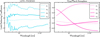 |
Fig. A.1 Wavelength-dependent limb-darkening coefficients for LHS 1140 b. Left: Coefficients c1–c4 of the four-parameter law obtained with LDTK (Parviainen & Aigrain 2015) using PHOENIX specific intensities, showing strong small-scale structure inherited from spectral lines. Right: Corresponding coefficients from our gray/Planck atmosphere approximation, yielding a smooth, line-free wavelength dependence that we adopt for the self-consistent ECLIPSE-Xλ simulations. |
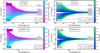 |
Fig. A.2 Supplementary analysis analogous to Figs. 1 and 2 but for the exoplanets K2-18 b (upper panels) and WASP-69 b (lower panels). The panels systematically explore the effect of varying the temperature contrast (left panels) and the filling factor (right panels). These supplementary figures confirm trends identified for LHS 1140 b while also highlighting the distinct stellar host type dependence (M-dwarf vs. K-type stars) of systematic biases between ECLIPSE-Xλ and TLSE. The dashed lines serve as reference markers, providing a visual support for interpreting variations in the data. |
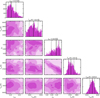 |
Fig. A.3 Posterior distributions for the stellar-contamination parameters of LHS 1140 b from the ECLIPSE-Xλ fit with limb darkening included. The panels show the 1D and 2D marginals for the spot filling factor (fspot), spot temperature (Tspot), facula filling factor (ffac), facula temperature (Tfac), and photospheric temperature (Tphot). Diagonal panels display the 1D histograms with the median and 16th–84th percentile intervals marked by solid and dashed vertical lines, respectively. Off-diagonal panels show the corresponding 2D credible regions, with darker shades indicating higher posterior density. Numerical summaries of these posteriors are reported in Table 2. |
All Tables
All Figures
|
Fig. 1 Wavelength-dependent errors between ECLIPSE-Xλ and the R-TLSE (Eq. (6)) for LHS 1140 b, computed using a fixed filling factor (fhet = 0.15) and a temperature contrast (ΔT) varying from −300 K (spots) to +300 K (faculae). The largest discrepancies arise in the optical range (500–800 nm), where steep limb-darkening gradients drive optical biases. The dashed lines mark reference levels at −50, −20, −10, 10, 20, and 50 ppm, serving as a visual aid to highlight variations in the data. By construction, positive values of the error indicate that R-TLSE predicts a shallower transit depth than ECLIPSE-Xλ (overcorrecting stellar contamination), while negative values correspond to a deeper R-TLSE transit (under-correcting contamination). |
| In the text | |
|
Fig. 2 Discrepancies, defined by Eq. (6), as a function of fixed temperature contrast (Tstar ± 300) and with the filling factor (fhet) varied from 0.01 to 0.15. Positive errors (R-TLSE overestimation) dominate for cool spots, while negative errors (R-TLSE underestimation) arise for hot faculae. Extreme cases (e.g., fhet = 0.15, ΔT = ±300 K) show maximal divergence. The dashed lines delineate boundaries at −50, −20, −10, 10, 20, and 50 ppm. |
| In the text | |
|
Fig. 3 2D parameter space exploration showing the discrepancies (Eq. (6)) at a representative wavelength of 600 nm. Each panel corresponds to a different exoplanetary system: LHS 1140 b (left panel), K2-18 b (middle panel), and WASP-69 b (right panel). Color scales indicate the difference between our model and the R-TLSE correction equation, as a function of filling factor and temperature contrast. |
| In the text | |
|
Fig. 4 Effect of the active region’s spatial position on the stellar disk for LHS 1140 b, illustrating the wavelength-dependent error between ECLIPSE-Xλ and R-TLSE. Each curve corresponds to a different temperature of the active region (spot or facula). The four panels examine positions gradually shifting from close to disk center (15° latitude, 0° longitude) toward the limb (35° latitude, 35° longitude). A sign inversion emerges at intermediate positions beyond the optical wavelengths (right panel, first row). The lower panels depict more extreme cases with active regions placed even closer to the limb, showing that the sign-inversion boundary moves to shorter wavelengths, significantly altering and reducing errors in the optical regime, while further limb positioning exacerbates R-TLSE inaccuracies due to enhanced limb darkening and foreshortening. Positive errors mean that R-TLSE predicts a shallower transit than ECLIPSE-Xλ (overcorrecting contamination), whereas negative errors mean that R-TLSE predicts a deeper transit (under-correcting contamination). |
| In the text | |
|
Fig. 5 Comparison between ECLIPSE-Xλ and the R-TLSE approximation for the JWST/NIRISS SOSS transmission spectrum of LHS 1140 b. Top: combined R ~ 100 NIRISS spectrum (gray points with error bars), together with the best-fitting stellar-contamination models. The magenta curve shows the self-consistent ECLIPSE-Xλ fit that includes wavelength-dependent limb darkening, the cyan curve shows the corresponding fit with limb darkening set to zero (LDCs = 0), and the black curve reproduces the TLS-only stellar-contamination model from the R-TLSE reference retrieval (see Cadieux et al. 2024). The small-scale structure along the model curves follows atomic and molecular absorption bands in the underlying PHOENIX spectra: TiO/VO and metal lines dominate in the optical, while broad features in the NIR are mainly shaped by H2O bands and CO absorption complexes longward of ~2.2 μm, i.e., precisely the wavelength ranges where exoplanet transmission spectra are usually interpreted in terms of H2O, CH4, and CO absorption. Bottom: 1D marginal distributions for the stellar-contamination parameters in the ECLIPSE-Xλ fits, for the cases with limb darkening (top row, magenta) and with LDCs= 0 (bottom row, cyan). From left to right, panels show the filling factor and temperature of spots (fspot, Tspot) and faculae (ffac, Tfac). Vertical lines indicate the median (solid) and 16th–84th percentile (dashed) intervals reported in Table 2. |
| In the text | |
|
Fig. A.1 Wavelength-dependent limb-darkening coefficients for LHS 1140 b. Left: Coefficients c1–c4 of the four-parameter law obtained with LDTK (Parviainen & Aigrain 2015) using PHOENIX specific intensities, showing strong small-scale structure inherited from spectral lines. Right: Corresponding coefficients from our gray/Planck atmosphere approximation, yielding a smooth, line-free wavelength dependence that we adopt for the self-consistent ECLIPSE-Xλ simulations. |
| In the text | |
|
Fig. A.2 Supplementary analysis analogous to Figs. 1 and 2 but for the exoplanets K2-18 b (upper panels) and WASP-69 b (lower panels). The panels systematically explore the effect of varying the temperature contrast (left panels) and the filling factor (right panels). These supplementary figures confirm trends identified for LHS 1140 b while also highlighting the distinct stellar host type dependence (M-dwarf vs. K-type stars) of systematic biases between ECLIPSE-Xλ and TLSE. The dashed lines serve as reference markers, providing a visual support for interpreting variations in the data. |
| In the text | |
|
Fig. A.3 Posterior distributions for the stellar-contamination parameters of LHS 1140 b from the ECLIPSE-Xλ fit with limb darkening included. The panels show the 1D and 2D marginals for the spot filling factor (fspot), spot temperature (Tspot), facula filling factor (ffac), facula temperature (Tfac), and photospheric temperature (Tphot). Diagonal panels display the 1D histograms with the median and 16th–84th percentile intervals marked by solid and dashed vertical lines, respectively. Off-diagonal panels show the corresponding 2D credible regions, with darker shades indicating higher posterior density. Numerical summaries of these posteriors are reported in Table 2. |
| In the text | |
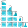 |
Fig. A.4 Same as Fig. A.3 but with limb darkening set to zero (LDCs = 0). |
| In the text | |
Current usage metrics show cumulative count of Article Views (full-text article views including HTML views, PDF and ePub downloads, according to the available data) and Abstracts Views on Vision4Press platform.
Data correspond to usage on the plateform after 2015. The current usage metrics is available 48-96 hours after online publication and is updated daily on week days.
Initial download of the metrics may take a while.