| Issue |
A&A
Volume 706, February 2026
|
|
|---|---|---|
| Article Number | A83 | |
| Number of page(s) | 14 | |
| Section | Cosmology (including clusters of galaxies) | |
| DOI | https://doi.org/10.1051/0004-6361/202556372 | |
| Published online | 02 February 2026 | |
Euclid: Early Release Observations – A combined strong and weak lensing solution for Abell 2390 beyond its virial radius★
1
Instituto de Física de Cantabria, Edificio Juan Jordá Avenida de los Castros 39005 Santander, Spain
2
Institute for Astronomy, University of Edinburgh, Royal Observatory Blackford Hill Edinburgh EH9 3HJ, UK
3
Aix-Marseille Université, CNRS, CNES, LAM Marseille, France
4
Institut d’Astrophysique de Paris, UMR 7095, CNRS, and Sorbonne Université 98 bis boulevard Arago 75014 Paris, France
5
Universität Innsbruck, Institut für Astro- und Teilchenphysik Technikerstr. 25/8 6020 Innsbruck, Austria
6
Department of Physics and Astronomy, University of Pennsylvania Philadelphia PA 19146, USA
7
Department of Astronomy, University of Massachusetts Amherst MA 01003, USA
8
Department of Astronomy, University of Geneva ch. d’Ecogia 16 1290 Versoix, Switzerland
9
STAR Institute, University of Liège, Quartier Agora Allée du six Août 19c 4000 Liège, Belgium
10
Department of Physics, Centre for Extragalactic Astronomy, Durham University South Road Durham DH1 3LE, UK
11
Department of Physics, Institute for Computational Cosmology, Durham University South Road Durham DH1 3LE, UK
12
Physics Program, Graduate School of Advanced Science and Engineering, Hiroshima University, 1-3-1 Kagamiyama Higashi-Hiroshima Hiroshima 739-8526, Japan
13
Hiroshima Astrophysical Science Center, Hiroshima University 1-3-1 Kagamiyama Higashi-Hiroshima Hiroshima 739-8526, Japan
14
Core Research for Energetic Universe, Hiroshima University, 1-3-1 Kagamiyama Higashi-Hiroshima Hiroshima 739-8526, Japan
15
School of Physics and Astronomy, University of Nottingham University Park Nottingham NG72RD, UK
16
INAF-Osservatorio di Astrofisica e Scienza dello Spazio di Bologna Via Piero Gobetti 93/3 40129 Bologna, Italy
17
INFN-Sezione di Bologna Viale Berti Pichat 6/2 40127 Bologna, Italy
18
Max Planck Institute for Extraterrestrial Physics Giessenbachstr. 1 85748 Garching, Germany
19
Kapteyn Astronomical Institute, University of Groningen PO Box 800 9700 AV Groningen, The Netherlands
20
Université de Strasbourg, CNRS, Observatoire astronomique de Strasbourg, UMR 7550 67000 Strasbourg, France
21
Max-Planck-Institut für Astronomie Königstuhl 17 69117 Heidelberg, Germany
22
Department of Physics, Université de Montréal 2900 Edouard Montpetit Blvd Montréal Québec H3T 1J4, Canada
23
Ciela Institute – Montréal Institute for Astrophysical Data Analysis and Machine Learning Montréal Québec, Canada
24
Mila – Québec Artificial Intelligence Institute Montréal Québec, Canada
25
Astrophysics Research Centre, University of KwaZulu-Natal Westville Campus Durban 4041, South Africa
26
School of Mathematics, Statistics & Computer Science, University of KwaZulu-Natal Westville Campus Durban 4041, South Africa
27
Department of Physics and Astronomy, University of British Columbia Vancouver BC V6T 1Z1, Canada
28
ESAC/ESA, Camino Bajo del Castillo, s/n. Urb. Villafranca del Castillo 28692 Villanueva de la Cañada Madrid, Spain
29
School of Mathematics and Physics, University of Surrey Guildford Surrey GU2 7XH, UK
30
INAF-Osservatorio Astronomico di Brera Via Brera 28 20122 Milano, Italy
31
IFPU, Institute for Fundamental Physics of the Universe Via Beirut 2 34151 Trieste, Italy
32
INAF-Osservatorio Astronomico di Trieste Via G. B. Tiepolo 11 34143 Trieste, Italy
33
INFN, Sezione di Trieste Via Valerio 2 34127 Trieste TS, Italy
34
SISSA, International School for Advanced Studies Via Bonomea 265 34136 Trieste TS, Italy
35
Dipartimento di Fisica e Astronomia, Università di Bologna Via Gobetti 93/2 40129 Bologna, Italy
36
Dipartimento di Fisica, Università di Genova Via Dodecaneso 33 16146 Genova, Italy
37
INFN-Sezione di Genova Via Dodecaneso 33 16146 Genova, Italy
38
Department of Physics “E. Pancini”, University Federico II Via Cinthia 6 80126 Napoli, Italy
39
INAF-Osservatorio Astronomico di Capodimonte Via Moiariello 16 80131 Napoli, Italy
40
Instituto de Astrofísica e Ciências do Espaço, Universidade do Porto, CAUP Rua das Estrelas PT4150-762 Porto, Portugal
41
Faculdade de Ciências da Universidade do Porto Rua do Campo de Alegre 4150-007 Porto, Portugal
42
European Southern Observatory Karl-Schwarzschild-Str. 2 85748 Garching, Germany
43
Dipartimento di Fisica, Università degli Studi di Torino Via P. Giuria 1 10125 Torino, Italy
44
INFN-Sezione di Torino Via P. Giuria 1 10125 Torino, Italy
45
INAF-Osservatorio Astrofisico di Torino Via Osservatorio 20 10025 Pino Torinese (TO), Italy
46
European Space Agency/ESTEC Keplerlaan 1 2201 AZ Noordwijk, The Netherlands
47
Institute Lorentz, Leiden University Niels Bohrweg 2 2333 CA Leiden, The Netherlands
48
Leiden Observatory, Leiden University Einsteinweg 55 2333 CC Leiden, The Netherlands
49
Mullard Space Science Laboratory, University College London Holmbury St Mary Dorking Surrey RH5 6NT, UK
50
INAF-IASF Milano Via Alfonso Corti 12 20133 Milano, Italy
51
INAF-Osservatorio Astronomico di Roma Via Frascati 33 00078 Monteporzio Catone, Italy
52
INFN-Sezione di Roma, Piazzale Aldo Moro, 2 – c/o Dipartimento di Fisica Edificio G. Marconi 00185 Roma, Italy
53
Centro de Investigaciones Energéticas, Medioambientales y Tecnológicas (CIEMAT) Avenida Complutense 40 28040 Madrid, Spain
54
Port d’Informació Científica, Campus UAB C. Albareda s/n 08193 Bellaterra (Barcelona), Spain
55
Institute for Theoretical Particle Physics and Cosmology (TTK), RWTH Aachen University 52056 Aachen, Germany
56
INFN section of Naples Via Cinthia 6 80126 Napoli, Italy
57
Institute for Astronomy, University of Hawaii 2680 Woodlawn Drive Honolulu HI 96822, USA
58
Dipartimento di Fisica e Astronomia “Augusto Righi” – Alma Mater Studiorum Università di Bologna Viale Berti Pichat 6/2 40127 Bologna, Italy
59
Instituto de Astrofísica de Canarias Vía Láctea 38205 La Laguna Tenerife, Spain
60
Jodrell Bank Centre for Astrophysics, Department of Physics and Astronomy, University of Manchester Oxford Road Manchester M13 9PL, UK
61
European Space Agency/ESRIN Largo Galileo Galilei 1 00044 Frascati Roma, Italy
62
Université Claude Bernard Lyon 1, CNRS/IN2P3, IP2I Lyon, UMR 5822 Villeurbanne F-69100, France
63
Institut de Ciències del Cosmos (ICCUB), Universitat de Barcelona (IEEC-UB) Martí i Franquès 1 08028 Barcelona, Spain
64
Institució Catalana de Recerca i Estudis Avançats (ICREA) Passeig de Lluís Companys 23 08010 Barcelona, Spain
65
UCB Lyon 1, CNRS/IN2P3, IUF, IP2I Lyon 4 rue Enrico Fermi 69622 Villeurbanne, France
66
Université Paris-Saclay, Université Paris Cité, CEA, CNRS, AIM 91191 Gif-sur-Yvette, France
67
Departamento de Física, Faculdade de Ciências, Universidade de Lisboa, Edifício C8 Campo Grande PT1749-016 Lisboa, Portugal
68
Instituto de Astrofísica e Ciências do Espaço, Faculdade de Ciências, Universidade de Lisboa Campo Grande 1749-016 Lisboa, Portugal
69
Université Paris-Saclay, CNRS, Institut d’astrophysique spatiale 91405 Orsay, France
70
INFN-Padova Via Marzolo 8 35131 Padova, Italy
71
Aix-Marseille Université, CNRS/IN2P3, CPPM Marseille, France
72
INAF-Istituto di Astrofisica e Planetologia Spaziali, Via del Fosso del Cavaliere 100 00100 Roma, Italy
73
Space Science Data Center, Italian Space Agency Via del Politecnico snc 00133 Roma, Italy
74
INFN-Bologna Via Irnerio 46 40126 Bologna, Italy
75
Institut d’Estudis Espacials de Catalunya (IEEC), Edifici RDIT Campus UPC 08860 Castelldefels Barcelona, Spain
76
Institute of Space Sciences (ICE, CSIC), Campus UAB, Carrer de Can Magrans s/n 08193 Barcelona, Spain
77
Universitäts-Sternwarte München, Fakultät für Physik, Ludwig-Maximilians-Universität München Scheinerstrasse 1 81679 München, Germany
78
INAF-Osservatorio Astronomico di Padova Via dell’Osservatorio 5 35122 Padova, Italy
79
Dipartimento di Fisica “Aldo Pontremoli”, Università degli Studi di Milano Via Celoria 16 20133 Milano, Italy
80
INFN-Sezione di Milano Via Celoria 16 20133 Milano, Italy
81
Institute of Theoretical Astrophysics, University of Oslo P.O. Box 1029 Blindern 0315 Oslo, Norway
82
Jet Propulsion Laboratory, California Institute of Technology 4800 Oak Grove Drive Pasadena CA 91109, USA
83
Department of Physics, Lancaster University Lancaster LA1 4YB, UK
84
Felix Hormuth Engineering Goethestr. 17 69181 Leimen, Germany
85
Technical University of Denmark Elektrovej 327 2800 Kgs. Lyngby, Denmark
86
Cosmic Dawn Center (DAWN), Denmark
87
NASA Goddard Space Flight Center Greenbelt MD 20771, USA
88
Department of Physics and Astronomy, University College London Gower Street London WC1E 6BT, UK
89
Department of Physics and Helsinki Institute of Physics Gustaf Hällströmin katu 2 00014 University of Helsinki, Finland
90
Université de Genève, Département de Physique Théorique and Centre for Astroparticle Physics 24 quai Ernest-Ansermet CH-1211 Genève 4, Switzerland
91
Department of Physics P.O. Box 64 00014 University of Helsinki, Finland
92
Helsinki Institute of Physics, Gustaf Hällströmin katu 2 University of Helsinki Helsinki, Finland
93
Laboratoire d’etude de l’Univers et des phenomenes eXtremes, Observatoire de Paris, Université PSL, Sorbonne Université, CNRS 92190 Meudon, France
94
SKA Observatory, Jodrell Bank, Lower Withington Macclesfield Cheshire SK11 9FT, UK
95
Centre de Calcul de l’IN2P3/CNRS 21 avenue Pierre de Coubertin 69627 Villeurbanne Cedex, France
96
Universität Bonn, Argelander-Institut für Astronomie Auf dem Hügel 71 53121 Bonn, Germany
97
Dipartimento di Fisica e Astronomia “Augusto Righi” – Alma Mater Studiorum Università di Bologna Via Piero Gobetti 93/2 40129 Bologna, Italy
98
Université Paris Cité, CNRS, Astroparticule et Cosmologie 75013 Paris, France
99
CNRS-UCB International Research Laboratory, Centre Pierre Binétruy, IRL2007 CPB-IN2P3 Berkeley, USA
100
University of Applied Sciences and Arts of Northwestern Switzerland, School of Engineering 5210 Windisch, Switzerland
101
Institut d’Astrophysique de Paris 98bis Boulevard Arago 75014 Paris, France
102
Institute of Physics, Laboratory of Astrophysics, Ecole Polytechnique Fédérale de Lausanne (EPFL), Observatoire de Sauverny 1290 Versoix, Switzerland
103
University Observatory, LMU Faculty of Physics Scheinerstrasse 1 81679 Munich, Germany
104
Telespazio UK S.L. for European Space Agency (ESA), Camino bajo del Castillo, s/n Urbanizacion Villafranca del Castillo Villanueva de la Cañada 28692 Madrid, Spain
105
Institut de Física d’Altes Energies (IFAE), The Barcelona Institute of Science and Technology Campus UAB 08193 Bellaterra (Barcelona), Spain
106
DARK, Niels Bohr Institute, University of Copenhagen Jagtvej 155 2200 Copenhagen, Denmark
107
Waterloo Centre for Astrophysics, University of Waterloo Waterloo Ontario N2L 3G1, Canada
108
Department of Physics and Astronomy, University of Waterloo Waterloo Ontario N2L 3G1, Canada
109
Perimeter Institute for Theoretical Physics Waterloo Ontario N2L 2Y5, Canada
110
Centre National d’Etudes Spatiales – Centre spatial de Toulouse 18 avenue Edouard Belin 31401 Toulouse Cedex 9, France
111
Institute of Space Science, Str. Atomistilor nr. 409 Măgurele Ilfov 077125, Romania
112
Dipartimento di Fisica e Astronomia “G. Galilei”, Università di Padova Via Marzolo 8 35131 Padova, Italy
113
Institut für Theoretische Physik, University of Heidelberg Philosophenweg 16 69120 Heidelberg, Germany
114
Institut de Recherche en Astrophysique et Planétologie (IRAP), Université de Toulouse, CNRS, UPS, CNES 14 Av. Edouard Belin 31400 Toulouse, France
115
Université St Joseph; Faculty of Sciences Beirut, Lebanon
116
Departamento de Física, FCFM, Universidad de Chile Blanco Encalada 2008 Santiago, Chile
117
Satlantis, University Science Park Sede Bld 48940 Leioa-Bilbao, Spain
118
Instituto de Astrofísica e Ciências do Espaço, Faculdade de Ciências, Universidade de Lisboa Tapada da Ajuda 1349-018 Lisboa, Portugal
119
Cosmic Dawn Center (DAWN)
120
Niels Bohr Institute, University of Copenhagen Jagtvej 128 2200 Copenhagen, Denmark
121
Universidad Politécnica de Cartagena, Departamento de Electrónica y Tecnología de Computadoras Plaza del Hospital 1 30202 Cartagena, Spain
122
Infrared Processing and Analysis Center, California Institute of Technology Pasadena CA 91125, USA
123
INAF, Istituto di Radioastronomia Via Piero Gobetti 101 40129 Bologna, Italy
124
Department of Physics, Oxford University Keble Road Oxford OX13RH, UK
125
Aurora Technology for European Space Agency (ESA), Camino bajo del Castillo, s/n Urbanizacion Villafranca del Castillo Villanueva de la Cañada 28692 Madrid, Spain
126
ICL, Junia, Université Catholique de Lille, LITL 59000 Lille, France
127
ICSC – Centro Nazionale di Ricerca in High Performance Computing, Big Data e Quantum Computing Via Magnanelli 2 Bologna, Italy
★★ Corresponding author: This email address is being protected from spambots. You need JavaScript enabled to view it.
Received:
11
July
2025
Accepted:
15
November
2025
Abstract
Euclid is currently mapping the distribution of matter in the Universe in detail via the weak lensing signature of billions of distant galaxies. The weak lensing signal is most prominent around galaxy clusters and can extend up to distances well beyond their virial radius, thus constraining their total mass. Near the centre of clusters, where contamination by member galaxies is an issue, the weak lensing data can be complemented with strong lensing data. Strong lensing information can also diminish the uncertainty due to the mass-sheet degeneracy and provide high-resolution information about the distribution of matter in the centre of clusters. Here we present a joint strong and weak lensing analysis of the Euclid Early Release Observations of the cluster Abell 2390 at z = 0.228. Thanks to Euclid’s wide field of view of 0.5 deg2, combined with its angular resolution in the visible band of 0.″13 and sampling of 0.″1 per pixel, we constrained the density profile in a wide range of radii, 30 kpc < r< 2000 kpc, from the inner region near the brightest cluster galaxy to beyond the virial radius of the cluster. We find relatively good consistency with earlier X-ray results based on assumptions of hydrostatic equilibrium and thus indirectly confirm the nearly relaxed state of this cluster. We also find consistency with previous results based on weak lensing data and ground-based observations of this cluster. From the combined strong + weak lensing profile, we derive the values of the viral mass M200 = (1.48 ± 0.29) × 1015 M⊙, and virial radius r200 = (2.05 ± 0.13 Mpc), with error bars representing one standard deviation. The profile is well described by a Navarro-Frenk-White model with a concentration c = 6.5 and a small-scale radius of 230 kpc in the 30 kpc < r< 2000 kpc range that is best constrained by strong lensing and weak lensing data. Abell 2390 is the first of many examples where Euclid data will play a crucial role in providing masses for clusters. The large coverage provided by Euclid, combined with the depth of the observations and high angular resolution, will allow us to produce similar results in hundreds of other clusters with rich strong lensing data that is already available.
Key words: gravitational lensing: strong / gravitational lensing: weak / galaxies: clusters: individual: Abell 2390 / dark matter
This paper is published on behalf of the Euclid Consortium.
© The Authors 2026
 Open Access article, published by EDP Sciences, under the terms of the Creative Commons Attribution License (https://creativecommons.org/licenses/by/4.0), which permits unrestricted use, distribution, and reproduction in any medium, provided the original work is properly cited.
This article is published in open access under the Subscribe to Open model. This email address is being protected from spambots. You need JavaScript enabled to view it. to support open access publication.
1. Introduction
Euclid, which is a mission of the European Space Agency (ESA), is currently surveying large portions of the sky (totalling ≈ 14 000 deg2 at the end of the survey) in one visible band, IE, and three (YE, JE, and HE) near-infrared bands. A summary of the Euclid mission is given in Euclid Collaboration: Mellier et al. (2025). One of Euclid’s primary goals is to extract accurate cosmological information with its high-quality shape measurements of ≈1.5 billion galaxies (Euclid Collaboration: Congedo et al. 2024). These shapes contain information about massive structures along the line of sight that produce a warping of space around them that distorts the apparent shape of background galaxies. Many of these galaxies will be found behind galaxy clusters, which allows us to constrain the masses of galaxy clusters using gravitational lensing. Euclid is expected to detect ≈106 clusters with masses above 1014 M⊙ and up to z ≈ 2 (Euclid Collaboration: Mellier et al. 2025). All of these clusters will imprint weak lensing signatures on background galaxies observed by Euclid and some of them will also act as strong gravitational lenses that produce multiple images of background galaxies.
Galaxy clusters are the most powerful gravitational lenses. The combined capabilities of Euclid regarding sensitivity of the visible imaging instrument (VIS) and near-infrared spectrometer and photometer (NISP) instruments (Euclid Collaboration: Cropper et al. 2025; Euclid Collaboration: Jahnke et al. 2025), spatial resolution, and sky coverage, allow us to extract the best weak lensing (WL) signal around these clusters. Some of the clusters observed by Euclid contain multiply lensed galaxies (or arcs), which can be used as constraints on the distribution of mass in the central regions of clusters, and also to break the mass-sheet degeneracy in the inner region constrained by strong lensing, provided that the lensed galaxies are at different redshifts (Saha 2000; Normann et al. 2025). At large radii, where only weak lensing data is available, some level of mass-sheet degeneracy may still introduce some uncertainty. Euclid’s spectroscopic capabilities are more limited in the crowded fields of galaxy clusters, which makes the determination of redshifts for these strongly lensed arcs a challenging task. However, many of the most prominent galaxy clusters observed by Euclid have already been observed by other space telescopes, including the Hubble Space Telescope (HST), and to a lesser degree the James Webb Space Telescope (JWST), together with ground-based telescopes that were used to estimate the redshifts of many of these strongly lensed galaxies. The ancillary strong lensing (SL) data available on these clusters (catalogues of spectroscopically confirmed multiply lensed galaxies) present a unique opportunity to combine precise SL data in the inner core of massive clusters with Euclid’s WL data extending far beyond the virial radius of each cluster. Such combinations of SL and WL data have already been performed in the past.
Earlier efforts combined space-based data for the SL constraints with ground-based data for the WL constraints (Broadhurst et al. 2005; Limousin et al. 2007; Oguri et al. 2009; Sereno & Umetsu 2011; Umetsu et al. 2016; Chiu et al. 2018; Abdelsalam et al. 1998; Bradač et al. 2006,
Umetsu et al. 2010; Jauzac et al. 2012; Wong et al. 2017), but in such cases the quality of the WL data was affected by seeing, which limits the accuracy of the shape measurements, as well as the depth of the observations. In other cases, only space-based data were used but these are restricted to small areas around the central region of the cluster, which therefore limits the results (Niemiec et al. 2023; Cha et al. 2024; Zitrin et al. 2015; Chiu et al. 2018; Patel et al. 2024). A recent compilation of methods used in the literature for joint weak and strong lensing analysis can be found in Normann et al. (2025).
Euclid data are a very valuable addition to pre-existing SL datasets, since they provide the sky coverage that is lacking in earlier space-based observations of clusters while being unaffected by the atmospheric effects that plague ground-based WL observations. Clusters at relatively low redshift with known multiply lensed galaxies are of particular interest. Low-redshift clusters have more background galaxies behind them and cover larger areas that can be easily covered by Euclid.
One such low-redshift galaxy cluster lens, Abell 2390 (or A2390), was observed as part of the Performance Verification phase of Euclid in late 2023. The targets observed during this campaign form a subset of observations known as the Euclid Early Release Observations (ERO), which were made public in May 2024. A description of the Euclid ERO programme is given in Cuillandre et al. (2025). The preliminary results on A2390 were presented in Atek et al. (2025), where a first analysis of the WL data was included. However, the results presented in Atek et al. (2025) do not take advantage of new photometric redshift estimates for galaxies in the Euclid image.
A2390 is a massive cluster at z = 0.228. From earlier work, its virial mass is estimated to be M200 ≈ 1.7 × 10¹⁵ M⊙ and it has an estimated velocity dispersion of σv ≈ 1100 km s−1 (Carlberg et al. 1996). Lens models for A2390 were derived in the past from ground-based observations and HST images (Pierre et al. 1996; Frye & Broadhurst 1998; Pelló et al. 1999; Swinbank et al. 2006; Richard et al. 2008) but in all cases were restricted to strong lensing. Chandra X-ray observations show A2390 as a cool-core cluster with a temperature kBT = (11.5 ± 1.5) keV in the outskirts (Allen et al. 2001). Good agreement is found between the inferred mass profile (under the assumption of hydrostatic equilibrium) and a Navarro–Frenk–White (NFW) profile with scale radius 0.8 Mpc and concentration c ≈ 3.3 (Allen et al. 2001).
More recently, additional evidence of a massive cooling flow towards the brightest cluster galaxy (BCG) is discussed in Alcorn et al. (2023) based on extended line emission found surrounding the BCG. Furthermore, ALMA observations reveal a massive concentration of molecular gas around the BCG, coincident with the X-ray and optical emissions (Rose et al. 2024). Radio observations of A2390 suggest past merger activity and the presence of polarised radio emission at the edges of the cluster (Bacchi et al. 2003). Finally, high-resolution LOFAR images of A2390 show double-tailed emission around the BCG, which strongly suggests the presence of an active galactic nucleus at its centre (Savini et al. 2019).
The paper is organised as follows. In Sect. 2 we describe the weak and strong lensing data used in this work. In Sect. 3 we discuss the algorithm WSLAP+ (Diego et al. 2005, 2007) used to combine the weak and strong lensing data and derive the mass distribution. We present our main results in Sect. 4. We finally conclude in Sect. 5. We adopt a flat cosmological model with Ωm = 0.3 and H0 = 70 km s−1 Mpc−1. For this model, and at the redshift of the lens (z = 0.228), 1″ = 3.65 kpc. For a different cosmological model, our results would vary by a small percentage. Most notably, lensing masses scale with the Hubble constant as H0−1, so for the Planck Collaboration VI (2020) model with H0 = 67.4 km s−1 Mpc−1 the cluster mass would be 3.86% higher than the values derived with H0 = 70 km s−1 Mpc−1 in this work.
2. Euclid and ancillary data on A2390
Our WL measurements come entirely from the new Euclid data. Here we summarise their main characteristics and refer the interested reader to Schrabback et al. (2025) for further details. Euclid observations of this cluster were carried out on November 28th 2023. The 5σ limiting magnitudes of the stacked images in the 4 Euclid filters are IE = 27.01 for VIS (in apertures with diameter  ) and YE = 25.18, JE = 25.22, HE = 25.12 for the NISP images (apertures with diameter
  ).
).
The photometric information (and derived photometric redshifts) were obtained after combining information from Euclid and ground-based ancillary data, in particular data from Subaru/Suprime-Cam (Miyazaki et al. 2002) in the bands B, V, Rc, i, Ic, and z′ (covering ≈ 28′ × 34′), and Canada-France-Hawaii Telescope (CFHT) Megacam u band. Both datasets complement Euclid observations with photometric measurements, relevant for the estimation of photometric redshifts. The ground-based data do not cover the full extent of the Euclid imaging, so we restricted our main analysis to a smaller square area of  where ground-based data are available and photometric redshifts are most reliable. This area is approximately 2.5 times smaller than the entire field of view of our Euclid data, but is perfectly centred on the galaxy cluster. A2390 is at low Galactic latitude (b ≈ −28°), where cirrus emission is significant. Photometry and shape measurements are performed over the ‘denebulised’ images, where the contribution from cirri has been reduced. The PSF was modeled with PSFex (Bertin 2011), and the mask from Atek et al. (2025) is used, after expanding it with extended low-redshift galaxies. Photometric redshifts are derived from Euclid and ground-based data using Phosphoros (Euclid Collaboration: Paltani et al. 2024), specifically developed for the Euclid Science Ground Segment and based on the code LePhare (Arnouts et al. 1999; Ilbert et al. 2006). In addition, a self-organizsing map approach combining all photometric information (ground-based and space-based data), and callibrated with COSMOS data, is also used to construct the distribution of galaxies as a function of redshift, n(z). See Schrabback et al. (2025) for details.
In this work we use weak lensing measurements from a subsample of background galaxies (from our photometric redshift catalogue) observed by Euclid. We refer to this subsample as the clean catalogue that was produced by vetoing galaxies that are likely members of A2390 or foreground galaxies. The clean catalogue is built after matching and merging three independent shape measurements: SE++ (Bertin et al. 2022; Kümmel et al. 2022); KSB+ (Kaiser & Squires 1993; Kaiser et al. 1995; Luppino & Kaiser 1997; Hoekstra et al. 1998; Erben et al. 2001; Schrabback et al. 2010); and LensMC (Euclid Collaboration: Congedo et al. 2024). This catalogue is the basis of the main weak + strong lensing analysis. In appendix A we show results obtained from the raw catalogue where no vetoing of galaxies is applied. The raw catalogue still suffers from contamination from foreground and member galaxies and it is included here only for illustration purposes. For the clean catalogue we find a number density of sources with reliable shear measurements between ≈10 and ≈50 galaxies per square arcminute. This number density is representative of the expected source density for weak lensing in Euclid. For comparison, the number density in the raw catalogue before removing foreground and member galaxies is approximately twice as large.
For the SL portion of the data, we relied on previous studies of this cluster with HST. We used the SL sample from Richard et al. (2008, 2021) that complements previously known redshifts of prominent arcs in the cluster with new spectroscopic estimates from the Multi Unit Spectroscopic Explorer (MUSE). The SL constraints are shown as coloured circles in Fig. 1, where the number indicates the ID of the family of multiple images from the same background galaxy. The lensed galaxies cover a wide range in redshift between z = 0.5346 (system 4) to z = 4.877 (system 7). The giant arc to the east (system 1) is at z = 1.036, and for illustration purposes we show the critical curve derived from our SL + WL model at that redshift, which nicely intersects this arc close to its middle point (as expected). The redshifts of each system are shown in the top left portion of the figure, with numbers in parentheses indicating the system ID with that redshift. Figure 1 also shows the critical curve at z = 4.05 (see Sect. 4).
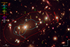 |
Fig. 1. Colour composite image (Red = NISP JE + YE + HE, Green = HST-ACS-F850LP, Blue = VIS IE) of the central region of A2390. The circles mark the position of the spectroscopic sample of SL constraints from Richard et al. (2008, 2021) colour coded by their spectroscopic redshift (indicated in the upper left). The number next to each small circle is the ID for each family of counterimages. We show the critical curves from the SL + WL model in cyan at zs = 1.036 and red at zs = 4.05. The image covers |

3. A joint SL + WL solution with WSLAP+
WSLAP+ was first described in Diego et al. (2005) and was originally developed to obtain the mass of galaxy clusters in a free-form way. That is, with no assumptions about the distribution of mass. The code was later expanded in Diego et al. (2007) to include weak lensing measurements as additional constraints. A further development is presented in Sendra et al. (2014) where the code migrated from its native free-form nature to a hybrid type of modelling where prominent member galaxies are added into the lens model with a mass distribution that matches the observed light distribution. The total mass of the member galaxies is the only free parameter, which is adjusted as part of the optimisation process. The addition of member galaxies plays a double role. On the one hand, it adds small-scale mass fluctuations that cannot be captured by the free-form part of the model. On the other hand, member galaxies act as a regularisation factor, anchoring the solution to a stable point in the space of solutions and reducing the problem of overfitting the data (see Sendra et al. 2014), which can otherwise produce spurious structures around clusters as described in Ponente & Diego (2011). The code has been validated with realistic lensing simulations (Meneghetti et al. 2017), used to reconstruct multiple lens models including all six Hubble Frontier Fields models based on HST data (Diego et al. 2016; Vega-Ferrero et al. 2019), and more recently to model clusters observed with the James Webb Space Telescope (Diego et al. 2023, 2024). WSLAP+ is well suited to fit rich lensing datasets where many constraints are available, as in the case of MACS0416 where WSLAP+ is used to fit the largest (to date) number of strong lensing constraints (observed positions of lensed galaxies) in a single galaxy cluster (more than 300, Diego et al. 2024). The free-form and hybrid nature of WSLAP+ is also appropriate for combining SL and WL data, since the optimisation of the solution is carried by simultaneously fitting the SL and WL constraints. WSLAP+ was previously used to combine SL and WL data in the well studied Abell 1689 cluster combining SL data from HST with WL data from Subaru (Diego et al. 2015). After the implementation in Sendra et al. (2014), additional improvements were made, such as the inclusion of critical points as constraints (see below). The description given here is the most up-to-date formulation of the code.
WSLAP+ is based on a simple decomposition of the deflection field, α, as a superposition of NG two-dimensional Gaussians (other decompositions have been tested, including polynomials, but the Gaussian decomposition provides the most robust results). Under this decomposition, the deflection α at a given position θ is computed as the sum of Gaussians placed at specific predetermined positions. These positions define a grid where the Gaussians are placed. The width of each Gaussian is also determined by the grid as separation between neighbouring grid points:
 (1)
(1)
where mi(θi,θ) is the mass contained in the Gaussian mass distribution at position θi and integrated out to the position θ. Factors Dds, Dos, and Dod are the angular diameter distances from the deflector to the source, from the observer to the source, and the observer to the deflector, respectively. The positions of the NG Gaussian functions, θi, define a grid that can be either regular in shape or follow an irregular distribution, with a higher density of points in the central region, where SL constraints are present, and the WL signal is stronger. A regular distribution of grid points represents a flat prior on the mass distribution since it makes no assumptions about the distribution of mass. The irregular grid is equivalent to a prior on the mass, where more mass is expected in regions where the grid has higher density. For situations like the ones discussed in this paper, where the centre of the lens is well determined from SL constraints, the use of the irregular grid is well motivated. Nevertheless, the irregular grid that we use is derived after a first optimisation performed with the regular grid, which results in an initial map of the mass distribution. The irregular grid samples this mass distribution and increases the number density of grid points in the portions of the lens plane with more mass, while reducing the total number of grid points, NG, and hence the number of free parameters. The distribution of the grid is shown in Fig. 2. The width of the Gaussians range between about 1′ near the centre to about 2′ near the edges. In the central 4′×4′ region constrained by SL (and marked with a yellow rectangle in Fig. 2) we increase the resolution even further by adding 123 smaller Gaussians with widths ranging from 12″ near the BCG galaxy to 40″ near the edges of the central 4′×4′ region. Combined with the 208 large-scale Gaussians that cover the larger  region, the total number of Gaussians is 331. We tested the solution with different grid configurations with varying number of grid points, Ng. For solutions where 250 ≲ Ng ≲ 400 we find small variation in the solution. Lens models derived with Ng < 250 start to degrade in resolution while models derived with Ng > 400 introduce artefacts, specially at large radii (noise overfitting).
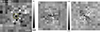 |
Fig. 2. Multi-scale grid used for binning the shear measurements in the clean catalogue. The grid is centred on the cluster. Left: Number of galaxies per square arcminute in each bin when only considering galaxies in the tomographic bins 3–10 described in Schrabback et al. (2025). The smallest bins in the centre are approximately 1′ × 1′ while at the edges the bins are |


For each SL constraint (or position θ), we have two equations similar to Eq. (1), one for the x-component and one for the y-component of θ. Given Nθ lensing constraints, the lens equation (β = θ − α) can be written in algebraic form
 (2)
(2)
where θx and θy are both an array of dimension Nθ containing the observed x and y coordinates of the Nθ SL arcs. βx and βx are each arrays of dimension Ns containing the unknown coordinates (x and y) of the Ns sources, and M is another array of dimension NG cells containing the unknown masses of the Gaussians in the grid. Finally, the matrices Θx and Θy each have dimension Nθ × NG and are known once the SL constraints and grid positions are determined. The terms of this matrix are the individual elements appearing in Eq. (1), with the masses mi of each grid point set to 1 × 10¹⁵ M⊙ at large distances from the grid points. Near each grid point, this mass is set by a Gaussian distribution,
 (3)
(3)
Adding member galaxies to the Gaussian grid decomposition of the mass can also be expressed in same the algebraic form as Eq. (2), with the only difference being that the mass of the member galaxies is a superposition of layers, with each layer containing a group of galaxies having similar light-to-mass ratio. The minimum number of layers is 1 and the maximum is the number of member galaxies considered, or lens planes in cases where line of sight effects need to be considered. For this work we adopt the simplest scenario where all member galaxies have the same light-to-mass ratio so there is only one layer containing all member galaxies.
The WL constraints can also be described in terms of differences of the deflection field and have a similar algebraic description to Eq. (2), only in this case the left column contains the observed shear measurements (γ1 and γ2) and on the right-hand side there is no β term,
 (4)
(4)
Similarly, member galaxies contribute to the shear with a similar system of linear equations as in Eq. (4). Since observations measure the reduced shear, g = γ/(1 − κ), WSLAP+ uses a previous solution (transformed into κ) to compute the matrix elements in Eq. (4). This is an important correction in regions of the lens plane where κ is more significant (i.e., near the centre of the lens). This process is iterated twice to ensure consistency between κ and the reduced shear. The shear is computed for each of the grid points in Fig. 2 by taking a weighted average of the individual shears of all galaxies falling in each square bin. The weights are a byproduct of the code LensMC used to measure shapes (Euclid Collaboration: Congedo et al. 2024). The resulting shear measurements are shown in the middle and right panels of Fig. 2. Similarly, we compute the weighted mean redshift for each square bin and from the same galaxies. This mean redshift is different for each square bin and is used in the definition of the terms Γ1 and Γ2 in Eq. (4). In both cases (mean shear and mean redshift per square bin), we exclude galaxies in the first tomographic bin from Schrabback et al. (2025). This excludes likely foreground and member galaxies from the average signal. Finally, to avoid unstable non-linearities near regions of high convergence (κ ≈ 1), we ignore the shear measurements in the 3 × 3 inner bins shown in the left panel of Fig. 2. This portion of the lens plane is well constrained by SL measurements.
The latest improvement to WSLAP+ was the addition of the position of critical curves, based on the observed position of arcs merging at the critical curves and their orientation. We do not use critical point information in this work but we include a brief description here for completion. In Diego et al. (2022, Appendix A.2) it is shown how, after a suitable rotation, the critical point information can also be described as a linear transformation of the deflection field in a form similar to the previous linear equations,
 (5)
(5)
where λ1 = κ + γ1R and λ2 = γ2R, with κ the lens model convergence at the critical point and γ1R, γ2R the shear at the same position but after a suitable rotation in the observed direction of the arc. After this rotation λ1 = 1 and λ2 = 0 at the critical points. The values of λ1 and λ2 can be used as additional constraints, as demonstrated in Diego et al. (2022) that used these additional constraints to improve the lens model near the lensed star “Godzilla” (at z = 2.37).
Combining all the available constraints, we can define a global system of linear equations that contains SL, WL, and critical point information (when available):
 (6)
(6)
where we show the explicit structure of the matrix. All terms in the 2 × 2 tensor are matrices, as described in Eqs. (2), (4), and (5). We also include here the terms associated with the member galaxies, such as C on the right-hand side, which is a multiplicative factor to the fiducial mass adopted for member galaxies. The upper index M or C refers to the matrices that are multiplying the M or C terms in the vector of unknown variables. The ij elements in the matrix Ix are 1 if the θi pixel contains a constraint from the βj source, and are 0 otherwise. The 0 matrix denotes the null matrix. Equation (6) can be written in the more compact form
 (7)
(7)
where Φ is an array containing the observed positions of the arcs, critical points at different redshifts, and binned shear measurements, Γ is the known non-square matrix in Eq. (6), and X is the solution we seek; This is, a vector with all the unknowns: masses in the Gaussian decomposition (M); multiplicative factors for the fiducial mass of the member galaxies (C); and source positions (βx and βy).
Even though the number of variables is often larger than the number of constraints, a direct inversion of the linear system of Eq. (7), X = Γ−1Φ, is in principle possible through singular value decomposition (which also works for non-square matrices) and after ignoring the terms associated with the smallest eigenvalues. However, the solutions obtained following this method are in general quite noisy. A better approach is to define the residual array
 (8)
(8)
and find the minimum of the scalar function  , where 𝒞 is the covariance matrix, which can be approximated by a diagonal matrix with terms σSL−2, σCP−2, and σWL−2, where σSL, σCP, and σWL are the uncertainties in the SL positions, critical point position, and WL shear measurements. Although not thoroughly tested yet with WSLAP+, off-diagonal terms in the covariance matrix can also be included, thus resulting in more precise solutions, but we ignore these terms here, since they are usually much smaller than diagonal terms.
For this cluster, we do not use critical point positions as constraints. For σSL we adopt an uncertainty of  or two pixels in the VIS images. For the shear measurements, we consider contributions from statistical shear measurements and from large-scale structure (Jain & Seljak 1997; Hoekstra et al. 1998); that is,
 (9)
(9)
where σstat is the average ellipticity of Nshear galaxies that are found in a given bin,
 (10)
(10)
where we assumed that the typical ellipticity of a galaxy before being sheared is 25%. For σLSS, we follow Jain & Seljak (1997), where for our cosmological model and assuming zs = 1.5, we find
 (11)
(11)
where Δ is the size of the bins (in arcmin) used to average the shear (see Fig. 2). For the model reconstruction, we assume a mean redshift per bin for the weak lensing measurements corresponding to the mean of Dds/Dos from the WL catalogue in each of the WL bins. This value fluctuates from WL bin to WL bin and it is in the range 0.6 ≲ Dds/Dos ≲ 0.7.
By construction, the minimum of f(R) is also a solution of the linear system of Eq. (7). This can be proven by simply setting the derivative of f(R) to zero. The minimum of f(R) can be found by fast algorithms such as the bi-conjugate gradient, but this can result in unphysical solutions where the masses in the Gaussian decomposition (or elements Xi in the solution array X) can be negative. Instead, we use a somewhat slower but more robust quadratic programming algorithm that seeks the minimum with the physical constraint Xi > 0, that is, the Gaussian masses, the mass of the member galaxies, and the source, positions all have to be positive (see Diego et al. 2005, for details). The positive nature of the masses is obvious. For the source positions, we define the origin of coordinates in the bottom-left corner of the field of view considered. With this choice, all positions are always positive in this frame of reference, so the requirement Xi > 0 is meaningful. In practice, since we are making the assumption that the distribution of mass is well represented by a superposition of Gaussian functions, and we know that this assumption must be wrong to some degree, we are not interested in the minimum of f(R), but in a value of f(R) close enough to the minimum, but above it by some value ϵ. Without the addition of member galaxies, WSLAP+ can recover solutions with very small values of ϵ. These solutions can be affected by artefacts, such as spurious rings of dark matter (Ponente & Diego 2011), which try to compensate for the imperfect original assumption with an imperfect solution. In earlier versions of WSLAP+, the optimisation had to be stopped when f(R) < ϵR, with ϵR playing the role of a regularisation term. Fortunately, the addition of member galaxies reduces, and in practical terms, eliminates this problem, since the optimisation reaches a point where the addition of more fluctuations in the Gaussian masses is anchored by the fixed mass distribution inside the member galaxies. This results in f(R) converging to a constant value (see Sendra et al. 2014).
4. Derived SL + WL lens model
We derived a series of solutions considering the same set of SL constraints, but with the three WL catalogues described in Sect. 2 (SE++, LensMC, and KSB+), and produced independently from the same Euclid data (see Schrabback et al. 2025, for details). To explore the range of solutions that are consistent with the data, we also varied the initial guess in the optimisation process. This initial guess introduces a degree of randomness in the derived solution, which is important to explore. Regions in the lens plane playing a less significant role in fitting the data are poorly constrained and suffer from a memory effect where the value they adopt after the optimisation correlates with the random value assigned in the first step of the optimisation. This happens for instance at relatively large distances from the centre of the cluster, where the WL signal is weakest, and can be partially described by the lensing effect from the central overdensity, thus requiring little or no mass in the outskirts of the cluster. This is a form of non-classical mass-sheet degeneracy where non-uniform distributions, for instance a ring of mass around the lens can have a small impact near the centre of the lens but larger in the outskirts. We explored this range of solutions for just one of the WL clean catalogues (LensMC). Most of the variability in the derived solution comes from the initial guess, and not the WL catalogue that is similar in all three cases as shown by Schrabback et al. (2025). Hence, solutions derived with the other two catalogues (SE++, and KSB+) exhibit a similar degree of variability.
We optimised the mass in the lens plane with WSLAP+ for the three WL clean catalogues (SE++, LensMC, and KSB+) and the fixed set of SL constraints. The mass profile obtained from each catalogue (centred in the BCG) is shown in Fig. 3. As described in the previous section, the lensing mass is obtained as a superposition of 2D Gaussian functions plus the re-scaled 2D distribution of the light of member galaxies. Hence, no profile is assumed for the cluster in Fig. 3. The horizontal dot-dashed line in the bottom shows the critical density of the Universe at z = 0.23 projected along 4 Mpc (roughly twice the virial radius). The three profiles, derived with the same initial guess, are shown as coloured lines and demonstrate excellent consistency among them, with small differences in the inner 10 kpc, which is the range unconstrained by SL measurements (or WL data). The derived profile is also in excellent agreement with the profile derived using strong lensing data only but a parametric model for the mass distribution (Abriola et al. 2025). In Fig. 3 we also compare the derived SL + WL profiles with an NFW profile (Navarro et al. 1996). This profile is given in its canonical form:
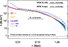 |
Fig. 3. Surface mass density (Σ) profiles as a function of radius (r) centred on the BCG for the three WL clean catalogues. Two NFW profiles are shown in black-grey. The dotted black line is the NFW derived from X-rays assuming hydrostatic equilibrium. The short-dashed black line is an NFW that fits the SL + WL model in the region that is best constrained by the SL + WL data. The light-blue band shows the 1σ variability in the LensMC profile when we change the initial guess in the SL + WL optimisation algorithm. The dashed dark-blue curve is the joint SL + WL solution when we use the raw LensMC in a larger field of view and with a minimal selection of objects (see Appendix A). |
 (12)
(12)
where the normalisation factor, ρo, is such that the mean density within the radius r200 is 200 times the critical density at redshift z, ρcrit(z):
 (13)
(13)
where δc is a constant that depends on the concentration parameter, c, and H(z) the Hubble parameter at redshift z. Since the radial profile is computed assuming circular bins, we assumed a spherical halo for the projected NFW profile. We found that the profile is reasonably well reproduced by an NFW with concentration parameter c = 6.5 and a relatively small-scale radius rs = 230 kpc (black dashed curve in the figure). This is higher than the concentration derived by Allen et al. (2001) based on Chandra data (c ≈ 3, black dotted curve in the figure), but our best-fit NFW model agrees better with the ones derived from Subaru WL data, c ≈ 6.4 (Oguri et al. 2010) and c ≈ 6.2 (Okabe et al. 2010). A posterior analysis in Okabe & Smith (2016) finds  . This lower concentration is partially explained by the fact that Okabe et al. (2010) used blue galaxies, which give a higher concentration (and lower masses) due to contamination of surrounding galaxies.
The range of possible solutions obtained when we vary the initial guess is shown as a light blue band in Fig. 3, which can be seen only at large radii (R ≳ 1 Mpc) since at smaller radius the light-blue region is very thin. As expected, the model is less constrained at larger radii, where the WL signal is weakest. The low-end of the range of profiles is obtained when the initial guess for the optimisation is set to random normal variables with a small dispersion (σG = 1011 M⊙) in the initial guess for the mass of the Gaussians. The high-end of the profile range is obtained when the initial guess is allowed to have larger masses (σG = 4 × 10¹¹ M⊙). In both cases, Gaussians in the outskirts of the cluster play a smaller role in fitting the observed WL data (and no role in the SL portion of the data). They are poorly optimised, maintaining values closer to their original value (memory effect). Part of the uncertainty at large radii shown by the blue band can be attributed to the mass-sheet degeneracy which is affecting more the WL portion of the data. As the initial guess varies between small and large values of σG, this is similar to applying a constant sheet of mass that retains some of its value at large radius while it is better constrained at small radii (by the SL portion of the data). This is similar to the more general ring-like degeneracy studied in Liesenborgs et al. (2008), but see also Ponente & Diego (2011) for a discussion of these artefacts.
From the range of possible models (light-blue shaded area), we can estimate the range of values for the virial radius, r200. Instead of relying on an analytical fit to the observed profiles, we computed the mass density from the derived SL + WL profiles inside a cylinder of radius R and length L = 2R along the line of sight. Then we defined r200 as the radius of the cylinder where the density inside the cylinder is 200 times the critical density. Using the cylindrical projection has the advantage of not relying on profiles to compute the overdensity in a sphere. Taking into account the dispersion of the profiles shown in Fig. 3 (light-blue region), we estimated the virial radius to be r200 = (2.05 ± 0.13) Mpc. This result is consistent with the low end of the range of virial radii derived from X-rays in Allen et al. (2001),  Mpc. Similarly, we found that the mass enclosed within the virial radius is M200 = (1.48 ± 0.29) × 1015 M⊙,
Comparison with results from the literature.
This is consistent with previous results for this cluster summarised in Table 1. The quantities Mvir and M200 are closely related but not identical, with the ratio between the two depending on cosmology and profile parameters. Mvir is often higher than M200 by around 20% (White 2001), a direct consequence of the smaller contrast in the definition of the virial mass and radius (178 versus 200 for the overdensity). Our mass estimate is consistent with masses derived from X-rays in Allen et al. (2001), and weak lensing masses derived from Weighing the Giants (from CFHT and Subaru data, Applegate et al. 2014), or Subaru WL estimates in Oguri et al. (2010), Okabe et al. (2010), and Okabe & Smith (2016). A higher mass is found in Hoekstra et al. (2015) as part of the Canadian Cluster Comparison Project (CCCP). This mass is based on a fit to an NFW profile (and also for h = 0.7). This large difference with our mass estimate cannot be attributed to the slightly different definitions of Mvir and M200. More recently, Sereno et al. (2025) estimates a dynamical mass based on the velocity dispersion of 353 members. The larger dynamical mass is partially due to the larger radius, r200 = 2.64 Mpc, considered in that work. The revision from Okabe & Smith (2016) yields also a higher mass, which may be connected with the lower concentration,  , found in that work. Our mass estimate is also in excellent agreement with the WL-only result (based on the same Euclid WL data) from Schrabback et al. (2025), that finds M200 = (1.45 ± 0.19)×1015, (1.64 ± 0.21)×1015, and (1.49 ± 0.21) × 1015 M⊙ for the SE++, LensMC, and KSB+ catalogues, respectively, assuming an NFW halo with a concentration c = 4.
The 2-dimensional distribution of mass in the central 4′×4′ region is shown in Fig. 4. It also shows the cluster members used as part of the lens model. The contours show the values of the convergence at zs = 3 and are mostly given by the smooth superposition of Gaussian functions. The smooth component peaks at the BCG position but is elongated in the NW-SE direction. A similar elongation is observed in the distribution of the X-ray emitting plasma, as shown in Fig. 5. In this case, the peak of the X-ray emission aligns with the position of the BCG, as well as with the maximum in the smooth component of the mass. A similar result is obtained when comparing with the intracluster light (ICL) in A2390, where the peak of the ICL matches well the X-ray and mass peaks (Ellien et al. 2025). The absence of additional peaks in the smooth distribution of mass, with a relatively small elongation, suggests a relaxed dynamical state of the cluster, which may explain the good agreement between the SL + WL profile and the X-ray profile obtained after assuming hydrostatic equilibrium. On the other hand, the large concentration inferred from the SL + WL analysis favours a prolate geometry for the cluster, with its main axis offset from the line of sight and along the NW-SE direction, which could also explain the observed elongation.
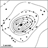 |
Fig. 4. Contours of the convergence at zs = 3. The member galaxies used in the model are also shown in black. The value of the convergence is indicated for some contours. We mark the value of κ = 0.5 with a thicker contour, which indicates the approximate position of the cluster critical curve at higher redshift. The value for the convergence in the last contour near the centre of the plot is κ = 1.06. |
The WL data over the large field of view of Euclid allow us to study the distribution of mass up to, and beyond, the virial radius. The two-dimensional distribution is shown in Fig. 6. The same NW-SE elongation found in the central region is also observed on larger scales, although less well defined, and with substructure deviating from a purely elliptical shape. A slightly higher concentration of mass can be observed in the NW section of the cluster, compared with the SE sector. A small dip in the mass is also observed SW of the BCG, which appears to correlate with a reduction in the X-ray emission. However, the X-ray data are still too noisy to extract solid conclusions about this possible correlation.
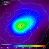 |
Fig. 5. Comparison of the convergence map in the centre of the cluster (shown in Fig. 4, colour scale) with the X-ray emission from Chandra (contours). For clarity, the convergence is saturated beyond κ = 1.2. |
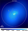 |
Fig. 6. Mass model (colour in log scale) vs. X-ray emission (contours) on a larger region and for the LensMC WL clean catalogue. Masses are given in M⊙ per pixel (one pixel = 2″ × 2″ or 53.92 kpc2). The white circle has a radius of 9.36 arcmin (2.05 Mpc at the redshift of the cluster), which marks the estimated virial radius of the cluster. X-ray contours correspond to 0.065, 0.12, 0.2, 0.5, 1, 2, 5, and 10 counts per pixel. |
5. Conclusions
We present the first SL + WL analysis of a galaxy cluster based on Euclid data (WL) and previous SL data. Euclid will provide similar measurements of the virial mass for hundreds of clusters and ancillary strong lensing high-quality data from telescopes such as HST or JWST is already available. The depth, large field of view, and resolution of Euclid images allow us to detect galaxies down to IE ≈ 27 mag, well beyond the virial radius of the cluster, and with a spatial resolution of  , well suited for measurements of the shear of individual high-redshift galaxies.
We combined the WL data from Euclid with preexisting HST SL data of the A2390 cluster, with the free-form hybrid method WSLAP+. In this approach, we model the distribution of mass as a smooth superposition of Gaussians and a more compact component that traces the light of the most prominent member galaxies in the cluster. For the WL data, we considered a clean catalogue, where we restricted ourselves to a subsample of galaxies with photometric redshifts based on Euclid and ground-based data.
From the combined SL + WL profile, we constrained the virial radius as r200 = (2.05 ± 0.13) Mpc, and virial mass as M200 = (1.48 ± 0.29) × 1015 M⊙, These constraints are in agreement with earlier X-ray and weak lensing results. Additionally, the derived mass profile is consistent with earlier results based on X-ray data that assume hydrostatic equilibrium, which suggests that the cluster must be close to equilibrium. However, the lensing profile does not match the X-ray derived profile exactly, which suggests that the cluster is not in perfect equilibrium. Interestingly, the lensing profile is below the X-ray profile, contrary to what is expected where the hydrostatic bias tends to bring the X-ray inferred mass below the lensing mass (see a recent result in Muñoz-Echeverría et al. 2024). We found a higher concentration for the cluster, which is consistent with the higher concentration found in previous WL studies from Subaru data. We also find consistency between the derived SL + WL virial mass and virial radius and earlier results. Part of the uncertainty in our results originates in the relatively small area of the ERO observations, which is further limited by the available ground-based photometry in a portion of this area. This affects the profile at large radii in particular, where the slope of the profile is more poorly constrained. Ground-based data are required to derive photometric redshifts for all the galaxies in the field and remove both foreground and member galaxies. Future studies based on Euclid data will cover larger areas and have improved photometric redshift estimates. This will be important to reduce the mass-sheet degeneracy that still affects the estimation of mass at large radii.
A2390 represents the first of many examples where Euclid’s high-quality WL data can be combined with available SL data to constrain the mass distribution of a cluster out to its virial radius. One of the main limitations of the current study is the lack of spectroscopic confirmation (from Euclid) of galaxies in the same field of view, since these were not available at the time of preparing this manuscript. Future results based on Euclid will take advantage of its spectroscopic capabilities, as well as additional ancillary observations, which will result in better removal of foreground galaxies and improved measurements of the WL signal and inferred virial mass.
Acknowledgments
The Euclid Consortium acknowledges the European Space Agency and a number of agencies and institutes that have supported the development of Euclid, in particular the Agenzia Spaziale Italiana, the Austrian Forschungsförderungsgesellschaft funded through BMK, the Belgian Science Policy, the Canadian Euclid Consortium, the Deutsches Zentrum für Luft- und Raumfahrt, the DTU Space and the Niels Bohr Institute in Denmark, the French Centre National d’Etudes Spatiales, the Fundação para a Ciência e a Tecnologia, the Hungarian Academy of Sciences, the Ministerio de Ciencia, Innovación y Universidades, the National Aeronautics and Space Administration, the National Astronomical Observatory of Japan, the Netherlandse Onderzoekschool Voor Astronomie, the Norwegian Space Agency, the Research Council of Finland, the Romanian Space Agency, the State Secretariat for Education, Research, and Innovation (SERI) at the Swiss Space Office (SSO), and the United Kingdom Space Agency. A complete and detailed list is available on the Euclid web site (www.euclid-ec.org). J.M.D. acknowledges support from projects PID2022-138896NB-C51 (MCIU/AEI/MINECO/FEDER, UE) Ministerio de Ciencia, Investigación y Universidades and SA101P24. We thank the anonymous referee for useful and constructive comments. The scientific results reported in this article are based in part on data obtained from the Chandra Data Archive (ObsId 4193, https://doi.org/10.25574/04193). The analysis is derived in part using data from the Subaru telescope, the Canada-France-Hawaii Telescope, and the Hubble space telescope.
References
- Abdelsalam, H. M., Saha, P., & Williams, L. L. R. 1998, AJ, 116, 1541 [NASA ADS] [CrossRef] [Google Scholar]
- Abriola, D., Lombardi, M., Grillo, C., et al. 2025, A&A, 704, A338 [NASA ADS] [CrossRef] [EDP Sciences] [Google Scholar]
- Alcorn, L. Y., Yee, H. K. C., Drissen, L., et al. 2023, MNRAS, 522, 1521 [Google Scholar]
- Allen, S. W., Ettori, S., & Fabian, A. C. 2001, MNRAS, 324, 877 [NASA ADS] [CrossRef] [Google Scholar]
- Applegate, D. E., von der Linden, A., Kelly, P. L., et al. 2014, MNRAS, 439, 48 [Google Scholar]
- Arnouts, S., Cristiani, S., Moscardini, L., et al. 1999, MNRAS, 310, 540 [Google Scholar]
- Atek, H., Gavazzi, R., Weaver, J., et al. 2025, A&A, 697, A15 [NASA ADS] [CrossRef] [EDP Sciences] [Google Scholar]
- Bacchi, M., Feretti, L., Giovannini, G., & Govoni, F. 2003, A&A, 400, 465 [NASA ADS] [CrossRef] [EDP Sciences] [Google Scholar]
- Bertin, E. 2011, ASP Conf. Ser., 442, 435 [Google Scholar]
- Bertin, E., Schefer, M., Apostolakos, N., et al. 2022, Astrophysics Source Code Library [record ascl:2212.018] [Google Scholar]
- Bradač, M., Clowe, D., Gonzalez, A. H., et al. 2006, ApJ, 652, 937 [CrossRef] [Google Scholar]
- Broadhurst, T., Takada, M., Umetsu, K., et al. 2005, ApJ, 619, L143 [NASA ADS] [CrossRef] [Google Scholar]
- Carlberg, R. G., Yee, H. K. C., Ellingson, E., et al. 1996, ApJ, 462, 32 [NASA ADS] [CrossRef] [Google Scholar]
- Cha, S., HyeongHan, K., Scofield, Z. P., Joo, H., & Jee, M. J. 2024, ApJ, 961, 186 [NASA ADS] [CrossRef] [Google Scholar]
- Chiu, I. N., Umetsu, K., Sereno, M., et al. 2018, ApJ, 860, 126 [NASA ADS] [CrossRef] [Google Scholar]
- Crittenden, R. G., Natarajan, P., Pen, U.-L., & Theuns, T. 2002, ApJ, 568, 20 [NASA ADS] [CrossRef] [Google Scholar]
- Cuillandre, J.-C., Bertin, E., Bolzonella, M., et al. 2025, A&A, 697, A6 [Google Scholar]
- Diego, J. M., Protopapas, P., Sandvik, H. B., & Tegmark, M. 2005, MNRAS, 360, 477 [Google Scholar]
- Diego, J. M., Tegmark, M., Protopapas, P., & Sandvik, H. B. 2007, MNRAS, 375, 958 [NASA ADS] [CrossRef] [Google Scholar]
- Diego, J. M., Broadhurst, T., Benitez, N., et al. 2015, MNRAS, 446, 683 [NASA ADS] [CrossRef] [Google Scholar]
- Diego, J. M., Broadhurst, T., Chen, C., et al. 2016, MNRAS, 456, 356 [NASA ADS] [CrossRef] [Google Scholar]
- Diego, J. M., Pascale, M., Kavanagh, B. J., et al. 2022, A&A, 665, A134 [NASA ADS] [CrossRef] [EDP Sciences] [Google Scholar]
- Diego, J. M., Meena, A. K., Adams, N. J., et al. 2023, A&A, 672, A3 [NASA ADS] [CrossRef] [EDP Sciences] [Google Scholar]
- Diego, J. M., Adams, N. J., Willner, S. P., et al. 2024, A&A, 690, A114 [NASA ADS] [CrossRef] [EDP Sciences] [Google Scholar]
- Ellien, A., Montes, M., Ahad, S. L., et al. 2025, A&A, in press, https://doi.org/10.1051/0004-6361/202554460 [Google Scholar]
- Erben, T., Van Waerbeke, L., Bertin, E., Mellier, Y., & Schneider, P. 2001, A&A, 366, 717 [NASA ADS] [CrossRef] [EDP Sciences] [Google Scholar]
- Euclid Collaboration (Congedo, G., et al.) 2024, A&A, 691, A319 [NASA ADS] [CrossRef] [EDP Sciences] [Google Scholar]
- Euclid Collaboration (Paltani, S., et al.) 2024, A&A, 681, A66 [NASA ADS] [CrossRef] [EDP Sciences] [Google Scholar]
- Euclid Collaboration (Cropper, M., et al.) 2025, A&A, 697, A2 [Google Scholar]
- Euclid Collaboration (Jahnke, K., et al.) 2025, A&A, 697, A3 [Google Scholar]
- Euclid Collaboration (Mellier, Y., et al.) 2025, A&A, 697, A1 [Google Scholar]
- Frye, B., & Broadhurst, T. 1998, ApJ, 499, L115 [Google Scholar]
- Hoekstra, H., Franx, M., Kuijken, K., & Squires, G. 1998, ApJ, 504, 636 [Google Scholar]
- Hoekstra, H., Herbonnet, R., Muzzin, A., et al. 2015, MNRAS, 449, 685 [NASA ADS] [CrossRef] [Google Scholar]
- Hu, W. 2000, Phys. Rev. D, 62, 043007 [NASA ADS] [CrossRef] [Google Scholar]
- Ilbert, O., Arnouts, S., McCracken, H. J., et al. 2006, A&A, 457, 841 [NASA ADS] [CrossRef] [EDP Sciences] [Google Scholar]
- Jain, B., & Seljak, U. 1997, ApJ, 484, 560 [Google Scholar]
- Jauzac, M., Jullo, E., Kneib, J.-P., et al. 2012, MNRAS, 426, 3369 [Google Scholar]
- Kaiser, N., & Squires, G. 1993, ApJ, 404, 441 [Google Scholar]
- Kaiser, N., Squires, G., & Broadhurst, T. 1995, ApJ, 449, 460 [Google Scholar]
- Kümmel, M., Álvarez-Ayllón, A., Bertin, E., et al. 2022, ArXiv e-prints [arXiv:2212.02428] [Google Scholar]
- Liesenborgs, J., de Rijcke, S., Dejonghe, H., & Bekaert, P. 2008, MNRAS, 386, 307 [Google Scholar]
- Limousin, M., Richard, J., Jullo, E., et al. 2007, ApJ, 668, 643 [NASA ADS] [CrossRef] [Google Scholar]
- Luppino, G. A., & Kaiser, N. 1997, ApJ, 475, 20 [Google Scholar]
- Meneghetti, M., Natarajan, P., Coe, D., et al. 2017, MNRAS, 472, 3177 [Google Scholar]
- Miyazaki, S., Komiyama, Y., Sekiguchi, M., et al. 2002, PASJ, 54, 833 [Google Scholar]
- Muñoz-Echeverría, M., Macías-Pérez, J. F., Pratt, G. W., et al. 2024, A&A, 682, A147 [NASA ADS] [CrossRef] [EDP Sciences] [Google Scholar]
- Navarro, J. F., Frenk, C. S., & White, S. D. M. 1996, ApJ, 462, 563 [Google Scholar]
- Niemiec, A., Jauzac, M., Eckert, D., et al. 2023, MNRAS, 524, 2883 [NASA ADS] [CrossRef] [Google Scholar]
- Normann, B. D., Solevåg-Hoti, K., & Schaathun, H. G. 2025, Eur. Phys. J. Plus, 140, 1175 [Google Scholar]
- Oguri, M., Hennawi, J. F., Gladders, M. D., et al. 2009, ApJ, 699, 1038 [NASA ADS] [CrossRef] [Google Scholar]
- Oguri, M., Takada, M., Okabe, N., & Smith, G. P. 2010, MNRAS, 405, 2215 [NASA ADS] [Google Scholar]
- Okabe, N., & Smith, G. P. 2016, MNRAS, 461, 3794 [Google Scholar]
- Okabe, N., Takada, M., Umetsu, K., Futamase, T., & Smith, G. P. 2010, PASJ, 62, 811 [NASA ADS] [Google Scholar]
- Patel, N. R., Jauzac, M., Niemiec, A., et al. 2024, MNRAS, 533, 4500 [Google Scholar]
- Pelló, R., Kneib, J. P., Le Borgne, J. F., et al. 1999, A&A, 346, 359 [Google Scholar]
- Pierre, M., Le Borgne, J. F., Soucail, G., & Kneib, J. P. 1996, A&A, 311, 413 [NASA ADS] [Google Scholar]
- Planck Collaboration VI. 2020, A&A, 641, A6 [NASA ADS] [CrossRef] [EDP Sciences] [Google Scholar]
- Ponente, P. P., & Diego, J. M. 2011, A&A, 535, A119 [NASA ADS] [CrossRef] [EDP Sciences] [Google Scholar]
- Richard, J., Stark, D. P., Ellis, R. S., et al. 2008, ApJ, 685, 705 [NASA ADS] [CrossRef] [Google Scholar]
- Richard, J., Claeyssens, A., Lagattuta, D., et al. 2021, A&A, 646, A83 [EDP Sciences] [Google Scholar]
- Rose, T., McNamara, B. R., Combes, F., et al. 2024, MNRAS, 528, 3441 [NASA ADS] [CrossRef] [Google Scholar]
- Saha, P. 2000, AJ, 120, 1654 [Google Scholar]
- Savini, F., Bonafede, A., Brüggen, M., et al. 2019, A&A, 622, A24 [NASA ADS] [CrossRef] [EDP Sciences] [Google Scholar]
- Schneider, P., van Waerbeke, L., Kilbinger, M., & Mellier, Y. 2002, A&A, 396, 1 [NASA ADS] [CrossRef] [EDP Sciences] [Google Scholar]
- Schrabback, T., Hartlap, J., Joachimi, B., et al. 2010, A&A, 516, A63 [CrossRef] [EDP Sciences] [Google Scholar]
- Schrabback, T., Congedo, G., Gavazzi, R., et al. 2025, A&A, submitted [arXiv:2507.07629] [Google Scholar]
- Sendra, I., Diego, J. M., Broadhurst, T., & Lazkoz, R. 2014, MNRAS, 437, 2642 [NASA ADS] [CrossRef] [Google Scholar]
- Sereno, M., & Umetsu, K. 2011, MNRAS, 416, 3187 [NASA ADS] [CrossRef] [Google Scholar]
- Sereno, M., Maurogordato, S., Cappi, A., et al. 2025, A&A, 693, A2 [NASA ADS] [CrossRef] [EDP Sciences] [Google Scholar]
- Stebbins, A. 1996, ArXiv e-prints [arXiv:astro-ph/9609149] [Google Scholar]
- Swinbank, A. M., Bower, R. G., Smith, G. P., et al. 2006, MNRAS, 368, 1631 [Google Scholar]
- Umetsu, K., Medezinski, E., Broadhurst, T., et al. 2010, ApJ, 714, 1470 [NASA ADS] [CrossRef] [Google Scholar]
- Umetsu, K., Zitrin, A., Gruen, D., et al. 2016, ApJ, 821, 116 [Google Scholar]
- Vega-Ferrero, J., Diego, J. M., & Bernstein, G. M. 2019, MNRAS, 486, 5414 [NASA ADS] [CrossRef] [Google Scholar]
- White, M. 2001, A&A, 367, 27 [NASA ADS] [CrossRef] [EDP Sciences] [Google Scholar]
- Wong, K. C., Raney, C., Keeton, C. R., et al. 2017, ApJ, 844, 127 [Google Scholar]
- Zitrin, A., Fabris, A., Merten, J., et al. 2015, ApJ, 801, 44 [Google Scholar]
This paper is published on behalf of the Euclid Consortium.
Appendix A: LensMC raw shear field analysis
The main WL analysis presented in this paper is based on the clean catalogue, which is limited in sky area (≈0.25deg2) and depth (IE < 26.5) in order to facilitate the photometric selection of background galaxies and estimation of their true redshift distribution. To illustrate the full potential of the Euclid LensMC shape catalogue we additionally include a simplified analysis of the measured raw shear field (without background selection, contamination correction, and redshift calibration) in this Appendix, going beyond these limitations both in terms of area and depth. Only a simple selection is done to remove unresolved objects (mostly stars) and obvious foreground objects with a larger half-light radius. This procedure removes 26.1% of the objects in the catalogue. After this simple selection, the typical number density of sources is larger by a factor approximately 2–3 than the number density of sources in the clean catalogue used for the main result. The shear from this raw sample is still expected to be contaminated by member galaxies and small foreground objects. This is particularly true for the central region within the virial radius where most member galaxies are expected to be found, but as we move away from the cluster centre, member galaxies should be less of an issue in terms of contaminating the shear. In order to test the content of lensing signal in the raw shear measurements, we perform two simple tests.
i) First, we computed the tangential and cross-components of the raw shear by weighting average of the corresponding ellipticity components in angular bins. The tangential and cross-components of the shear are computed adopting a point near the BCG as the centre, RA = 328.° 406, Dec = 17.° 6961. The tangential component of the raw shear is detected with a signal-to-noise ratio of S/N = 41 when combined over all bins up to 30 arcmin (or a factor about 3 times the estimated virial radius). Meanwhile, the cross component oscillates around zero, as shown in Fig. A.1.
ii) As a second test, from the raw shear measurements we computed the convergence map via the classic Kaiser–Squires inversion (Kaiser & Squires 1993). The map was originally estimated on a grid size of 12″, which is later smoothed via median filtering to 2′. We show the resulting decomposition into E and B modes (Stebbins 1996; Hu 2000; Crittenden et al. 2002; Schneider et al. 2002) in Fig. A.2. The cluster is detected with high significance in the E mode reconstruction, while the B mode reconstruction is consistent with noise. Similarly to the results obtained with the clean shear measurements, when using the raw shear measurements we find no evidence of substructure beyond the virial radius.
Finally, using the raw shear we recomputed the joint SL + WL solution on the larger field covered by the raw catalogue (an area approximately twice as large as the area covered by the clean shear catalogue). The result is shown as a dashed blue line in Fig. 1. The profile derived with the raw shear is clearly above the profile derived with the clean catalogue and has a smaller concentration, resembling more the profile derived from X-ray data (dotted line in the figure). The difference with the profile obtained using the clean catalogue (solid blue line) is likely due to contamination from member galaxies and foreground objects in the raw catalogue. Also, part of the difference may be due to the fact that in the case of the raw catalogue the relative weight of the shear data (with respect to the strong lensing constraints) is larger due to the increase in the number density of shear measurements per bin (see Eq. 10).
While the larger mass in the central region of the cluster may be attributed to contamination from member galaxies, the increase in mass in the dashed line profile is more noticeable at the outskirts of the cluster. Interpreting the increase in mass at larger radii is not trivial. This could still be due to contaminants to the WL signal, although we expect contamination to decrease significantly at larger radii. Alternatively, the difference may be due to the increase in the signal-to-noise ratio at larger radii, since the number density of galaxies is larger.
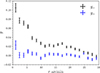 |
Fig. A.1. Tangential, and cross-components, (g+ and g×, respectively) of the raw shear estimates (without background selection and contamination correction) from the full-depth LensMC catalogue as a function of angular distance from the cluster centre. The signal is significant for r < 25′. The cross-shear, g×, is largely consistent with zero (except the first bin, heavily contaminated by member galaxies), which demonstrates the good control of systematic errors in this raw catalogue. |
 |
Fig. A.2. Convergence map reconstructed from the LensMC raw shear catalogue (without background selection and contamination correction), decomposed into E-modes (left) and B-modes (right). The alignment of the cluster mass in the SE-NW direction (left) is similar to the orientation found with the clean shear catalogue (Fig. 5). The absence of a clear B-mode signal in the right panel demonstrates the good control of systematic errors in this raw catalogue. |
All Tables
All Figures
|
Fig. 1. Colour composite image (Red = NISP JE + YE + HE, Green = HST-ACS-F850LP, Blue = VIS IE) of the central region of A2390. The circles mark the position of the spectroscopic sample of SL constraints from Richard et al. (2008, 2021) colour coded by their spectroscopic redshift (indicated in the upper left). The number next to each small circle is the ID for each family of counterimages. We show the critical curves from the SL + WL model in cyan at zs = 1.036 and red at zs = 4.05. The image covers |
| In the text | |
|
Fig. 2. Multi-scale grid used for binning the shear measurements in the clean catalogue. The grid is centred on the cluster. Left: Number of galaxies per square arcminute in each bin when only considering galaxies in the tomographic bins 3–10 described in Schrabback et al. (2025). The smallest bins in the centre are approximately 1′ × 1′ while at the edges the bins are |
| In the text | |
|
Fig. 3. Surface mass density (Σ) profiles as a function of radius (r) centred on the BCG for the three WL clean catalogues. Two NFW profiles are shown in black-grey. The dotted black line is the NFW derived from X-rays assuming hydrostatic equilibrium. The short-dashed black line is an NFW that fits the SL + WL model in the region that is best constrained by the SL + WL data. The light-blue band shows the 1σ variability in the LensMC profile when we change the initial guess in the SL + WL optimisation algorithm. The dashed dark-blue curve is the joint SL + WL solution when we use the raw LensMC in a larger field of view and with a minimal selection of objects (see Appendix A). |
| In the text | |
|
Fig. 4. Contours of the convergence at zs = 3. The member galaxies used in the model are also shown in black. The value of the convergence is indicated for some contours. We mark the value of κ = 0.5 with a thicker contour, which indicates the approximate position of the cluster critical curve at higher redshift. The value for the convergence in the last contour near the centre of the plot is κ = 1.06. |
| In the text | |
|
Fig. 5. Comparison of the convergence map in the centre of the cluster (shown in Fig. 4, colour scale) with the X-ray emission from Chandra (contours). For clarity, the convergence is saturated beyond κ = 1.2. |
| In the text | |
|
Fig. 6. Mass model (colour in log scale) vs. X-ray emission (contours) on a larger region and for the LensMC WL clean catalogue. Masses are given in M⊙ per pixel (one pixel = 2″ × 2″ or 53.92 kpc2). The white circle has a radius of 9.36 arcmin (2.05 Mpc at the redshift of the cluster), which marks the estimated virial radius of the cluster. X-ray contours correspond to 0.065, 0.12, 0.2, 0.5, 1, 2, 5, and 10 counts per pixel. |
| In the text | |
|
Fig. A.1. Tangential, and cross-components, (g+ and g×, respectively) of the raw shear estimates (without background selection and contamination correction) from the full-depth LensMC catalogue as a function of angular distance from the cluster centre. The signal is significant for r < 25′. The cross-shear, g×, is largely consistent with zero (except the first bin, heavily contaminated by member galaxies), which demonstrates the good control of systematic errors in this raw catalogue. |
| In the text | |
|
Fig. A.2. Convergence map reconstructed from the LensMC raw shear catalogue (without background selection and contamination correction), decomposed into E-modes (left) and B-modes (right). The alignment of the cluster mass in the SE-NW direction (left) is similar to the orientation found with the clean shear catalogue (Fig. 5). The absence of a clear B-mode signal in the right panel demonstrates the good control of systematic errors in this raw catalogue. |
| In the text | |
Current usage metrics show cumulative count of Article Views (full-text article views including HTML views, PDF and ePub downloads, according to the available data) and Abstracts Views on Vision4Press platform.
Data correspond to usage on the plateform after 2015. The current usage metrics is available 48-96 hours after online publication and is updated daily on week days.
Initial download of the metrics may take a while.